Western Arctic wintertime mixed-phase clouds: Observed modulation by sea ice conditions, long-term variabilities and trends

To assess the long-term interaction between sea ice conditions and Arctic mixed-phase cloud (MPC) properties, fourteen winter seasons of observations from the North Slope of Alaska are analysed. MPC properties are contextualized with respect to sea ice conditions by identifying the most relevant upstream sea ice sector influencing the observed clouds. A conical sector with a 6° azimuthal width and a 50 km radius, based on the direction of maximum water vapour transport (WVT) within the atmospheric boundary layer, is considered. The height of the WVT is used as indicator of its interaction with the cloud, enabling classification as either cloud-coupled or decoupled. MPC properties are further classified according to the presence of high or low pressure systems and analysed as a function of sea ice concentration (SIC). Results indicate which MPC properties exhibit significant changes as SIC decreases. The long-term time series reveal both positive and negative trends in MPC properties, depending on the WVT coupling status and the prevailing atmospheric pressure system. Statistically significant positive trends are found, suggesting increases in sea ice-MPC coupled liquid water path ($+\mathrm{35.0}\pm \mathrm{0.9}$ g m⁻² per decade), cloud base height ($+\mathrm{44.0}\pm \mathrm{0.7}$ m per decade) and cloud top temperature ($+\mathrm{2.2}\pm \mathrm{0.7}$ K per decade) under low pressure weather systems. Additionally, the evolution of MPC properties display cyclical characteristics, which are hypothesized to be in phase with climate oscillations like ENSO or PDO. Although the results support this hypothesis, establishing a direct causal link remains non-trivial.

1 Introduction

Climate physics has long established that increasing atmospheric greenhouse gas concentrations warms the atmosphere (Arrhenius, 1897; Hegerl, 2022). Observations over recent decades indicate that the Arctic is warming two to four times faster than the global average (Rantanen et al., 2022; Wendisch et al., 2023; Tan et al., 2023), a phenomenon known as Arctic amplification (AA) (Serreze and Francis, 2006; Serreze and Barry, 2011). Climate models attribute AA primary to external forcing, primarily the atmospheric lapse-rate feedback and sea ice loss. However, uncertainty in the magnitude of AA persist, largerly due to models' limited ability to simulate the sensitivity of Arctic sea ice loss to rising global temperatures (Notz and Community, 2020; Rantanen et al., 2022).

During Polar night, Arctic mixed-phase clouds (MPC) exert a positive cloud radiative effect (CRE), enhancing surface warming and contributing to sea ice decline (Shupe and Intrieri, 2004; Cox et al., 2015). The strength of this feedback depends on micro- and macro-physical cloud properties (Shupe and Intrieri, 2004; Tan and Storelvmo, 2019). As a result, improving the understanding of MPC's role in a changing Arctic – both in terms of their role in climate feedbacks and their representation in models – is a major research priority (Morrison et al., 2012; Korolev and Milbrandt, 2022; Tan et al., 2023, 2025; Schemann and Ebell, 2020; Hofer et al., 2024).

Recent studies highlight the importance of realistic cloud representation for simulating sea ice trend. Cesana et al. (2025), though focused on Antarctica, found that prescribing wind fields in climate models improves the simulation of sea ice and clouds variability compared to satellite observations. They emphasized that accurate cloud representation is crucial to capture the observed sea ice trends–challenge that current climate models still face. Large scale Pan-Arctic studies reveal contrasting cloud characteristics over sea ice versus open water: Palm et al. (2010) reported higher cloudiness frequency and geometric thickness of low level clouds over open ocean, while they found an increase of cloud geometrical thickness over open water. Li et al. (2020b) found that newly re-frozen sea ice areas can mitigate low level cloud development due to imbalanced heat and moisture fluxes. Furthermore, sea ice concentration (SIC) changes can alter the thermodynamic phase of wintertime MPC through convective heat transfer over leads and polynyas (Andreas and Cash, 1999). Papakonstantinou-Presvelou et al. (2022) found more ice crystals in low-level clouds over sea ice than over open water, attributing this to surface-specific aerosol types. While sea ice leads are identified as main sources of sea spray aerosols, their emission rates and drivers remain poorly quantified (Lapere et al., 2024).

Using synergistic atmospheric observations on-board the research vessel (RV) Polarstern during the year-long Multidisciplinary drifting Observatory for the Study of Arctic Climate MOSAiC expedition (2019–2020) (Shupe et al., 2022), Saavedra Garfias et al. (2023) proposed a physical mechanism linking local sea ice states in the vicinity of RV Polarstern to MPC properties above the ship. By leveraging a high-quality, high-resolution, satellite-derived sea ice lead fraction product specifically developed for MOSAiC along the RV Polarstern drifting path (von Albedyll et al., 2024), Saavedra Garfias et al. (2023) found that MPC properties – particularly liquid water path (LWP) – are positively correlated with upstream lead fraction when clouds are coupled to the sea ice leads via the water vapour transport (WVT). In contrast, ice water path (IWP) showed no significant correlation with lead fraction.

Most prior studies linking MPC and sea ice rely on either large-scale or short-term observations, limiting their utility for climate model evaluation. While models can capture some aspects of MPC, they often fail to accurately represent thermodynamic phase and ice/liquid water path (Schemann and Ebell, 2020; Pithan et al., 2014). Moreover, current climate models inadequately simulate how MPC properties evolve under a warming climate (Cesana et al., 2025; Nakanishi and Michibata, 2025). Thus, long-term, high-quality observations are paramount for climate model validation. Manaster et al. (2017) analysed over 20 years of multi-satellite data to estimate global liquid water path (LWP) trends over oceans, comparing them with CMIP5 models. Although their study excluded polar regions, their results are one of the few references for the long-term rate of change of LWP. They reported a positive LWP trends of about 1–2 g m⁻² per decade in the Southern Ocean and the North Pacific. They found that removing inter-annual variability, e.g. El Niño Southern Oscilation (ENSO), did not resolve model-observation discrepancies, suggesting ENSO is not the dominant driver–though other modes (e.g., Pacific Decanal Oscillation, PDO) may play a larger role.

This brings up two questions: Firstly, can the MOSAiC-based findings of Saavedra Garfias et al. (2023) – derived from a single winter in the central Arctic – be confirmed using for long-term observations in the Western Arctic? Secondly, are Arctic MPC properties modulated by climate variability modes not evident in short-term studies? Answering these questions advances our understanding of ocean-sea ice-atmosphere interaction and their feedbacks on Arctic cloud properties, providing critical insights for improving MPC representation in weather and climate models. To address this, the present study applies the methodology of Saavedra Garfias et al. (2023) to 14 winter seasons (2011–2024) of wintertime MPC observations at the ARM North Slope of Alaska (NSA) site in the Western Arctic.

The manuscript is structured as follows: Sect. 2 details the measurement site, instrumentation, data processing, and analysis methods. Section 3 presents results, including the modulation of MPC properties by sea ice conditions for the entire 14 years (Sect. 3.1), the year-to-year-variability (Sect. 3.2), and trends (Sect. 3.2.3), respectively. Section 4.3 discusses these findings in the context of MOSAiC results and their implications. Supplement includes detailed descriptions of data availability, statistical methods, climatological analysis, nomenclature description, and ancillary results.

2 Data and Methodology

The U.S. Department of Energy's Atmospheric Radiation Measurement (ARM) program (https://www.arm.gov/, last access: 9 May 2026.) provides long-term, high-quality observations for clouds and radiation at multiple sites around the world. For Arctic reseach, one of the few sources of quasi continuous, long-term observations is the ARM North Slope of Alaska (NSA) site, located in Utqiaǵvik, Alaska (71.323° N and 156.609° W), in the Western Arctic (Fig. 1). In this study, we use 14 winter seasons (1 November to 30 April) of NSA site observations to characterize mixed-phase clouds (MPC) and investigate how their properties are influenced by upstream sea ice conditions. To this end, we adapt and apply the methodology developed by Saavedra Garfias et al. (2023), hereafter referred to PSG23, to the ARM NSA site instrument suite, as described in the following section.

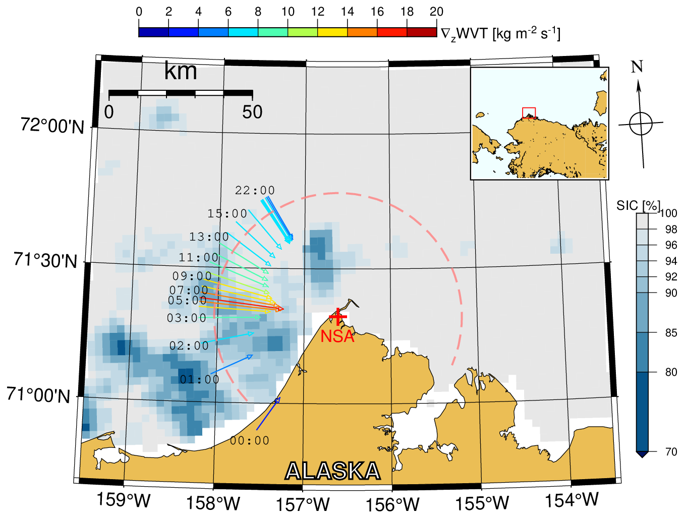
Figure 1 ARM's North Slope of Alaska NSA site (red cross: 71.23° N, 156.61° W) in Utqiaǵvik, Alaska (top right inlet). Right-bottom colour scale indicates the AMSR2 sea ice concentration (SIC) from 19 January 2019. Red-dashed 50 km semi-circle marks the sub-sector around NSA site considered in this study. The coloured radial arrows depict the direction of ∇_z𝚆𝚅𝚃 at selected times throughout the day for visualization purposes (see Sect. 2.4) as observed above NSA site. AMSR2 data courtesy of JAXA.

2.1 ARM atmospheric remote sensing instrumentation

The primary instruments used to characterize MPC are the ARM Ka-band zenith-pointing cloud radar (KAZR), the Vaisala CL31 cloud ceilometer (lidar), and a dual-frequency microwave radiometer (MWR). Moreover, atmospheric boundary layer (ABL) parameters and thermodynamic states are estimated from synergy between the ground-based infrared radiometer (GND_IRT) and regular radiosondes launched from the NSA site. Table 1 summarizes the instruments, relevant data products, spatial and temporal resolutions, and their corresponding references. A detailed timeline of data over the study period is provided in Fig. S14 (Sect. S4 in the Supplement). Additionally, satellite-derived sea ice observations are required to complement the atmospheric data for the application of the PSG23 method. The processing and merging of sea ice data with the atmospheric observations are explained in Sect. 2.3.

Zhang (2024)Cadeddu et al. (2024)Johnson et al. (2024)Toto and Giangrande (2024)Zhang et al. (2024)Jensen et al. (2024)Riihimaki et al. (2024)Shi et al. (2024)Melsheimer and Spreen (2019)Melsheimer and Spreen (2019)Melsheimer and Spreen (2019)O'Connor (2025)NOAA AO (2025)JPL ENSO (2025)JPL PDO (2025)

Table 1 Specifications of instrumentation, data products and their references used for this study. VAP refers to ARM's Value Added Product.

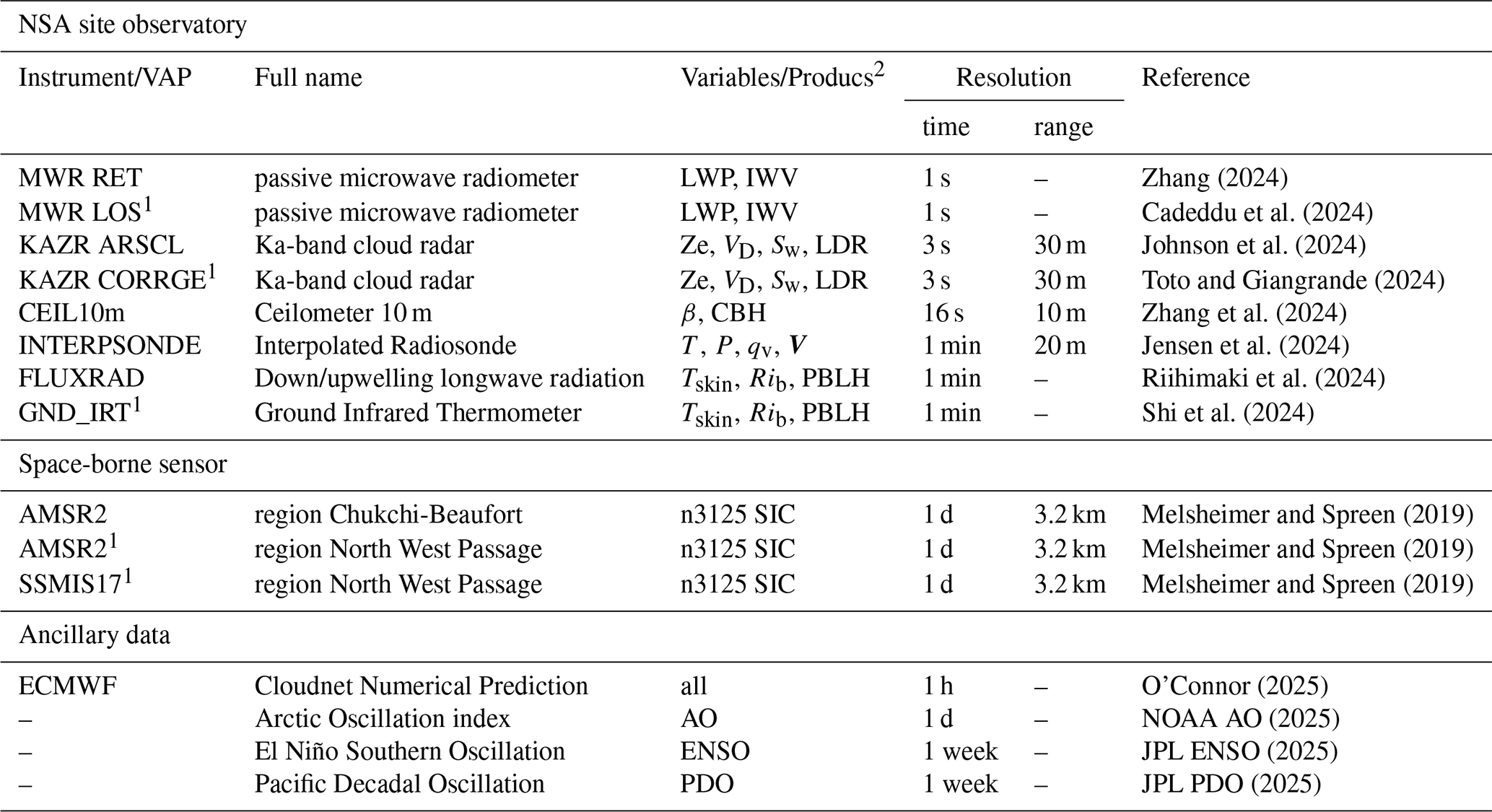
¹ Used as alternative to reduce data gaps. ² See Appendix E for full definition of acronyms.

2.2 Characterization of the cloudy atmosphere

Figure 2 illustrate the synergy of KAZR, ceilometer, and MWR observations for a case on 19 January 2019. These data, combined with thermodynamic profiles from the ECMWF numerical weather model (O'Connor, 2025) or radiosonde soundings, form the basis for classifying cloud thermodynamic phase and hydrometeor type. The retrieval algorithm used in this study is the state-of-the-art Cloudnet target classification algorithm (Illingworth et al., 2007; Tukiainen et al., 2020) version CloudnetPy 1.68.1 (Fig. 2d). Since ARM data are not natively compatible with CloudnetPy, the raw instrumentation data (Table 1) were pre-processed and adapted to meet input requirements (Saavedra Garfias, 2022). Beyond standard Cloudnet products, additional cloud and atmospheric properties are computed: atmospheric boundary layer height, cloud base and top heights, and cloud top temperature for each cloud layer. Readers are referred to PSG23 for details.

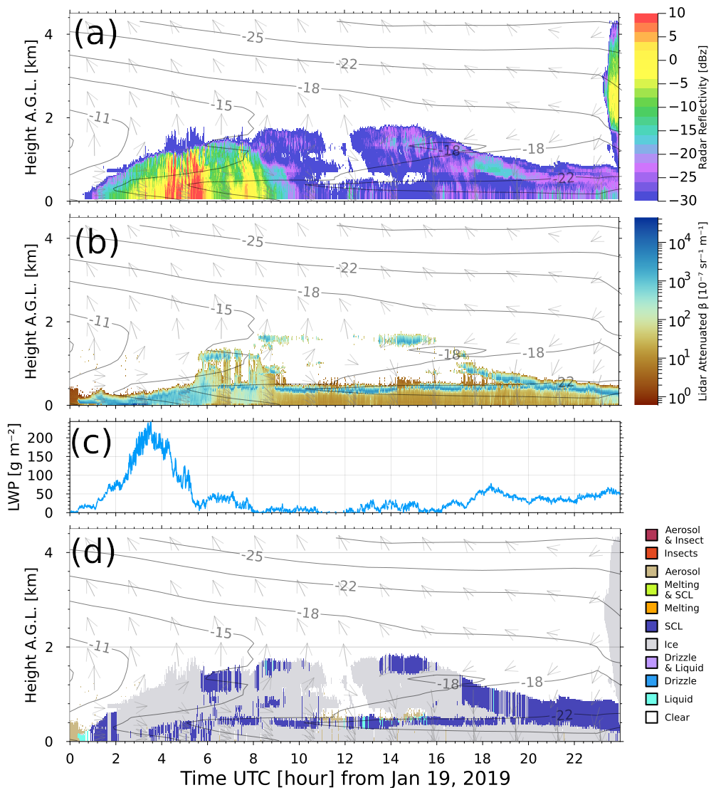
Figure 2 Synergistic ground-based remote sensing observations at NSA on 19 January 2019. Ka-band cloud radar (KAZR) reflectivity factor (a), ceilometer Vaisala CL31 attenuated backscattering coefficient β (b), dual-frequency MWR liquid water path (c), Cloudnet target classification (d) with supercooled liquid (SCL) in blue. Panels (a), (b) and (d) include profiles of the ECMWF numerical weather prediction model horizontal wind vector (arrows) and temperature (isotherms).

Accurate characterization of low-level Arctic stratus clouds is compromised when the liquid-containing cloud base lies below the radar's lowest detection range. As noted by Griesche et al. (2020), if the lidar signal is attenuated by a low-level liquid layer and no higher liquid layer is detected, Cloudnet classifies the entire profile as ice, leading a complete omission of LWP from the MWR (e.g., Fig. 2 02:00–03:30 UTC). However, if a higher liquid layer is present, the MWR LWP is distributed accordingly. Griesche et al. (2020, 2024) report that for the MOSAiC expedition such low-level stratus cases occur in over 25 % of observation time, with higher frequency in summer than winter. At the NSA site, the lidar can detect liquid clouds down to 10 m altitude, whereas the KAZR has a lowest detection range of 160 m (ARSCL) and 100 m (CORRGE), respectively (see references in Table 1). The present study finds that low-level clouds below the radar's detection threshold (160 m for ARSCL, 100 m for CORRGE) account for approximately 26 % and 22.5 % of observations, respectively. To mitigate this limitation, the dataset is adjusted via a flat extrapolation of radar reflectivity down to the lidar's lowest liquid detection altitude (10 m) prior to cloud characterization.

A key limitation of the Cloudnet target classification algorithm is its reliance on valid lidar signal for liquid cloud detection. As shown in Fig. 2 (02:00–04:00 UTC), complete attenuation of the lidar signal by low-level liquid layers results in the misclassification of higher supercooled liquid layer as ice. Consequently, liquid water content is underestimated, and ice-only clouds are overestimated. More advanced cloud radar Doppler spectra-based tools – such as those introduced by Kalesse-Los et al. (2022) and Schimmel et al. (2022) – can detect liquid beyond lidar signal attenuation, but their application would require extensive retraining on the NSA dataset and significant computation resources, which are beyond the scope of this study. As a result, the Cloudnet derived MPC dataset used here exhibits a low bias in liquid-phase detection, while ice-only clouds are overestimated.

The Cloudnet processing chain – applied to 14 years of NSA data – forms the basis for a merged dataset of macro- and micro-physical cloud properties, combined with sea ice conditions (see Sect. 2.3). This approach follows Saavedra Garfias and Kalesse-Los (2023), where MPC are retained only when both LWP and IWP exceed 5 g m⁻² in a single layer, minimizing uncertainties from retrieval algorithms due to instrument detection thresholds.

2.3 Characterization of sea ice conditions around NSA site

The PSG23 method originally used high-resolution (700 m) sea ice lead fraction (LF) derived from sea ice divergence from Synthetic Aperture Radar (SAR) satellite imagery specifically developed for the MOSAiC expedition (von Albedyll et al., 2024). However, such high-resolution LF products are not available for the multi-year NSA site observations. Instead, we use sea ice concentration (SIC) from the University of Bremen's publicly available satellite-based Arctic sea ice products (https://www.seaice.uni-bremen.de/start/, last access: 9 May 2026, e.g. Spreen et al., 2008; Melsheimer and Spreen, 2019) to characterize the ocean conditions surrounding the NSA site. The SIC product is retrieved from brightness temperatures measured by the Advanced Microwave Scanning Radiometer-2 (AMSR2) onboard the Global Change Observation Mission 1st GCOM-W1 satellite since autumn 2012. AMSR2 sea ice (ASI) provides daily SIC at 3.124 km polar stereographic grid resolution (see “Space-borne sensor” in Table 1) (Spreen et al., 2008). For this study, we use the “Chukchi-Beaufort” region (Fig. 1), centred at the NSA site and covering the western and eastern part of the Chukchi and Beaufort Seas. To identify the most relevant sea ice conditions for cloud interaction, we defined a 50 km radius semi-circular sector centred at NSA site (red dashed line in Fig. 1) spanning azimuths from −125 to 110°. This sector excludes the landward side (i.e. southerly inflow), ensuring that only clouds, with CTH ≤ 3 km, advected from open or ice-covered ocean areas are considered. This exclusion removes ∼ 8.1 % of the data, corresponding to clouds originating from land.

The mean and standard deviation of SIC are used. SIC is assumed to follow a truncated normal distribution with lower and upper truncation limits of 0 % and 100 %, respectively. The PSG23 method further restricts analysis to a ± 3° conical sector extending from the NSA site outwards up to 50 km and aligned with the upwind direction v_w of maximum vertical gradient of water vapour transport (∇_z𝚆𝚅𝚃), as described in Sect. 2.4. The mean sea ice concentration within the conical sector is denoted by SIC, whereas the mean sea ice concentration over the full 50 km semi-circular sector is denoted as SIC_⊙ (Fig. 3). The annual differences between these two metrics are shown in Fig. S1 (Sect. S1.1 in the Supplement).

Between 2011 and 2025, the Chuckchi-Beafort region experienced several winters with extraordinary low SIC (≲50 % in Figs. 3 and S1), including 2012/13, 2016/17, 2017/18, 2019/20, 2023/24, and 2024/25. These anomalies are likely linked to climatological variability and/or low latitude forcing. For example, Zhang et al. (2023) found that increased frequency of atmospheric rivers in winter correlates with reduced sea ice in the Barents-Kara seas. Atmospheric rivers prevent the sea ice recovering from summer melt and from growing to the climatologically expected sea ice coverage in winter. For the Chukchi-Beaufort region (2011 to 2020), atmospheric river frequency (averaged over November to April) has maximum values of 5.3 % in 2018/19, with intermediate value (2.6 %) in 2013/14, 2014/15, and 2019/20, and a minimum value of 0.2 % in 2015/16 (personal communication with Pengfei Zahng on 13 February 2024). The wintertime 2018–2019, despite moderate atmospheric river activity, saw a less frequent but still noticeable ${\mathrm{SIC}}_{\odot }\lesssim$ 50 % (Fig. S1), likely due to anomalous warm ocean waters driven by southerly winds and episodic atmospheric blocking over the Bering Sea in September 2018 – directly observed by the RV Mirai Arctic Expedition in November 2018 (Kodaira et al., 2020).

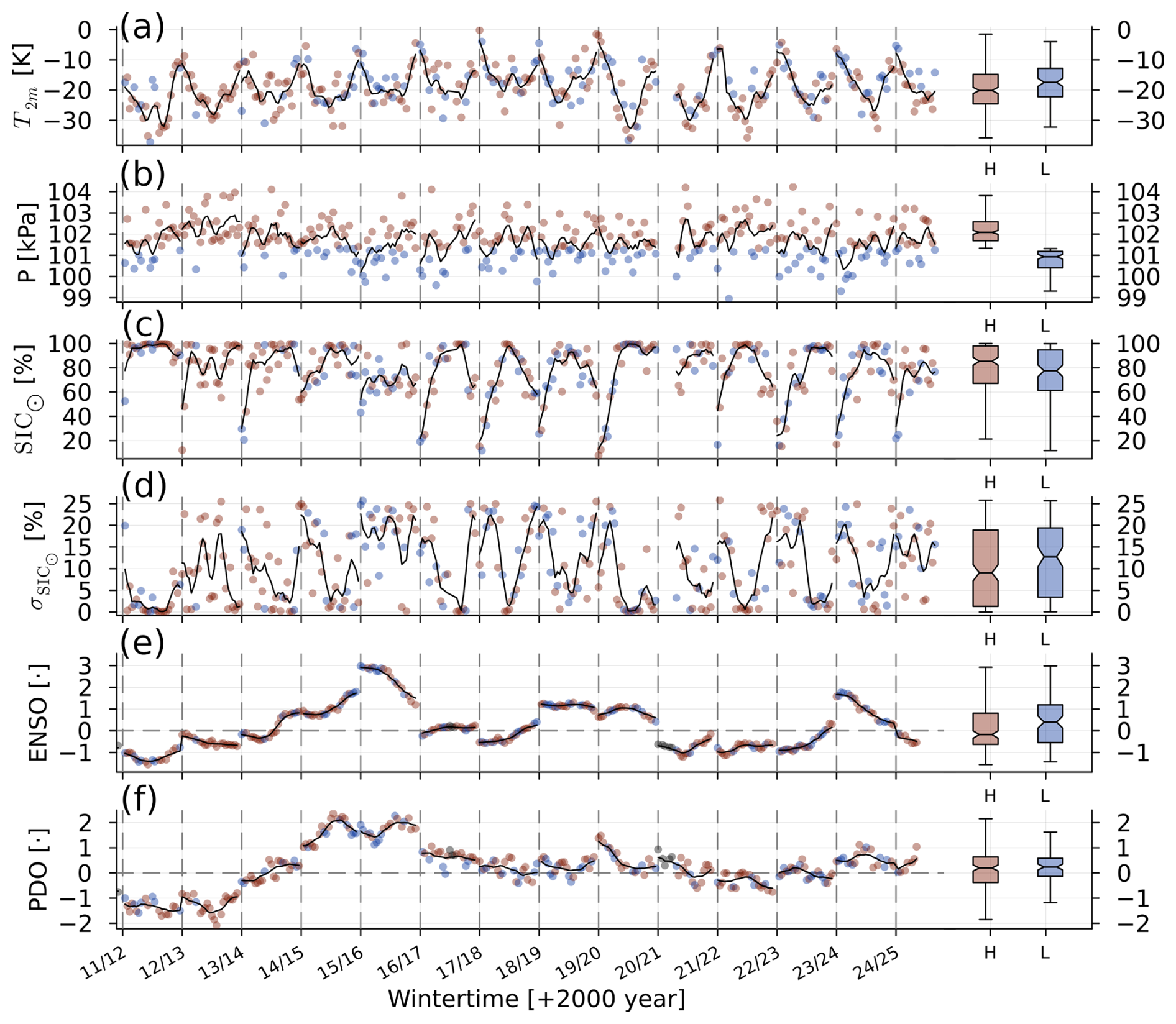
Figure 3 Wintertime climatology for the NSA site as time series from 2011 to 2024 for: (a) 2 m air temperature, (b) surface atmospheric pressure, (c) average SIC_⊙ within the whole 50 km semi-circle around NSA site, (d) standard deviation of SIC_⊙, (e) ENSO index, (f) PDO index. For visualization purposes the data is shown as weekly averages (circles), the solid black line is the weekly moving average. The vertical dashed lines indicate the jump from end of April to November, thus the apparent discontinuity at these lines is not physical. On the right of each panel the whole data distribution is shown as boxplot separated according to Eq. (2) for H- and L-pressure systems in light-red and light-blue, respectively.

2.4 Sea ice – atmosphere coupling via water vapour transport

Winter sea ice leads and polynyas act as localized sources of heat and moisture released to the atmosphere. Through convection and advection, these plumes can be transported downstream and influence cloud properties. To establish a physical link between sea ice and clouds, we apply the PSG23 methodology, using the water vapour transport (WVT) as a physical mechanism to link, akind a conveyor belt, the upstream sea ice conditions and the measured cloud properties above the NSA site (Saavedra Garfias et al., 2023). WVT is derived from radiosonde profiles and represents the magnitude and direction of water vapour flux and consists of several bands of different magnitudes along the vertical profile.

The PSG23 method identifies the most relevant WVT layer using its vertical profile gradient (∇_z𝚆𝚅𝚃 [kg m⁻² s⁻¹]) within the planetary boundary layer height (PBLH). The PBLH is constrained when the bulk Richardson number Ri_b≈1. The vertical gradient of ∇_z𝚆𝚅𝚃 is calculated using Eq. (1) (a detailed derivation is given in Saavedra Garfias et al., 2023).

$$\begin{array}{}\text{(1)}& {\mathrm{\nabla }}_z\mathtt{WVT}=-{\displaystyle \frac{{\mathrm{10}}^{\mathrm{2}}}{g}}|q_{\mathrm{v}}\cdot {\mathit{v}}_{\mathrm{w}}|{\displaystyle \frac{\mathrm{d}P}{\mathrm{d}z}}\end{array}$$

where ∇_z indicates the vertical gradient, g is the constant of gravity, with the specific humidity q_v [g kg⁻¹], horizontal wind speed v_w [m s⁻¹], and air pressure P [Pa] at altitudes z [m].

A cloud is classified as coupled (co) to the sea ice-WVT system if ∇_z𝚆𝚅𝚃 has a local maximum within the cloud mixing layer – defined by the cumulative variance of virtual potential temperature θ_v from cloud base/top height downwards/upwards until a threshold is exceeded. Otherwise, the cloud is classified as decoupled (de).

Within the ASI grid cells a conical sector (± 3°) is aligned with the upwind direction at the altitude of maximum ∇_z𝚆𝚅𝚃 (e.g., Fig. 1 where the radial arrows depict the direction of ∇_z𝚆𝚅𝚃 and their colour the magnitude). Only SIC values within this sector are used for analysis. At a given time the azimuth of the conical sector is governed by the upwind direction obtained from the altitude where ∇_z𝚆𝚅𝚃 reaches its maximum. Southerly winds (landward flow) are excluded. Figure S1 highlight a critical distinction: sea ice conditions in the full semi-circular sector differ significantly from those in the upwind conical sector. Thus, using large-scale SIC to infer cloud properties may lead to ill-posed correlations since not all sea ice conditions play a relevant role to explain observed cloud properties (e.g. Palm et al., 2010; Li et al., 2020a, b).

2.5 NSA site atmospheric pressure systems and climatology

The NSA site climatology is influenced by the persistent cyclonic activity in the north-western Pacific Ocean and anticyclonic systems over the Beaufort/Chukchi seas (Serreze et al., 1993; Serreze and Barry, 2014). Surface pressure serves as a proxy for synoptic-scale high (H-) or low (L-) pressure systems over NSA site (Fig. 3). Atmospheric air temperature and pressure are closely related to stability or instability in the atmosphere which strongly influences the formation of clouds. Local pressure systems are classified by the following steps: (i) a reference virtual isobaric surface P₀ is assumed to separate the H- or L-pressure observations, (ii) from the measured surface pressure and temperature, the relative height of the virtual isobar P₀ is determined. The relative height of P₀ is expressed in terms of geopotential height difference derived from the equation of state (Rogers and Yau, 1991):

$$\begin{array}{}\text{(2)}& \mathrm{\Delta }Z={\displaystyle \frac{R\stackrel{\mathrm{‾}}{T}}{g_{\mathrm{0}}}}\log \left({\displaystyle \frac{P_{\mathrm{0}}}{P}}\right)\end{array}$$

where R is the specific gas constant 287.05 J kg⁻¹ K⁻¹, g₀ the acceleration of gravity at the surface 9.81 m s⁻², $\stackrel{\mathrm{‾}}{T}$ the mean temperature within the layer [K], P₀ the reference isobar surface (in this case the mean sea level pressure of 101.32 k Pa), and P is the measured local surface pressure [kPa] at a given time. Δ Z is negative for H-pressure systems (i.e. P>P₀), and positive for L-pressure (i.e. P<P₀). $\stackrel{\mathrm{‾}}{T}$ is assumed to be the measured 2 m air temperature, and its effect is to adjust the magnitude of Δ Z when P departures considerably from the reference P₀.

From 2011 to 2024, surface pressures at NSA were slightly biased towards H-pressure (median: 101.69 kPa; and Inter-Quantile Region (IQR): 100.95–102.50 kPa), with H-pressure systems occurring 56.3 % of the time and L-pressure systems 43.7 % of the time. The distribution of Δ Z differs significantly between coupled and decoupled cases: Coupled: median $\mathrm{\Delta }Z=-\mathrm{9.45}$ m (IQR: −65.05 to 44.72 m); Decoupled: median -30.98 m (IQR: −86.95 to 18.74 m). This indicates that H-pressure systems favour decoupled cloud formation. Note that ΔZ reflects local conditions and does not replace synoptic-scale pressure systems from Western Arctic weather maps.

3 Results

NSA site wintertime (1 November to 30 April) observations from 2011 to 2024 were analysed in accordance with the methodology outlined in the previous sections. Results are presented after observations from the instruments listed in Table 1 were resampled to a common 1 min time resolution and clustered by high (ΔZ<0) and low (ΔZ≥0) pressure weather systems, as well as by coupled (co), and decoupled (de) status. Wintertime cloud properties are reported using two approaches: as a function of SIC, following Saavedra Garfias et al. (2023) (Sect. 3.1), and as time series over the 14 years (Sect. 3.2). Descriptive statistics are presented using the median (${\mathit{\mu }}_{\mathrm{1}/\mathrm{2}}$) and variability quantified by the median absolute deviation (MAD) defined as ${\mathit{\sigma }}_{\text{mad}}=\pm \mathrm{median}$ $\left(\left|X_i-{\mathit{\mu }}_{\mathrm{1}/\mathrm{2}}\right|\right)$. Additional statistical descriptors include the geometric mean (μ_g), the 25th, and 75th percentiles. Unless otherwise specified, results are reported as ${\mathit{\mu }}_{\mathrm{1}/\mathrm{2}}\pm {\mathit{\sigma }}_{\text{mad}}$.

3.1 Modulation of MPC properties as a function of SIC, coupling status, and pressure system

For the considered time period the cloud frequency of occurrence (FoO) were analysed. The total cloud FoO (Fig. 4, left bars) remains approximately constant at ∼75 % throughout the winter, with a dependency on SIC in the monthly distribution. For MPC (Fig. 4, right bars) the FoO decreases from ∼56 % in November to ∼40 % in April, with the largest contribution from SIC > 95 % occurring in January. Total cloud FoO (left bars) is derived from all observations with CTH ≤ 3 km and either MWR-LWP > 0 g m⁻² or IWP > 0 g m⁻², indicating detection of liquid or ice clouds. MPC occurrence is defined by simultaneous detection of liquid and ice by both MWR and radar. The persistent presence of SIC = 0 % in every month indicates the continuous occurrence of polynyas and leads during winter along the SIC semi-cone around the NSA site. It is important to note that the SIC values in Fig. 4 represent the average within a 50 km radius, 6° wide semi-cone, with the azimuth determined by direction of the maximum WVT.

The absolute values for total cloud and MPC are consistent with previous studies: Shupe et al. (2011) reported an annual total cloud FoO of ∼ 80 % at NSA, and Shupe et al. (2006) reported a MPC FoO of ∼ 40 % in fall.

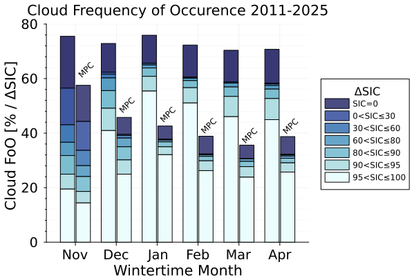
Figure 4 FoO for total (left bars) and mixed-phase clouds (right bars) per month for wintertime from 2011 to 2025. The FoO is based on cloud events in a month versus total days in a month.

To investigate the relationship between sea ice and cloud properties, the data were binned by SIC with bins centred at every 20th percentile. MPC properties are represented by the median ${\mathit{\mu }}_{\mathrm{1}/\mathrm{2}}$ and its MAD σ_mad within each SIC bin. For the following analysis, MPC detection were restricted to cases with LWP and IWP above 5 g m⁻² to reduce noise from minimum detectable retrieval uncertainties, similar as in PSG23.

Figure 5 presents the liquid water path (LWP), cloud droplet effective radius r_eff, ice water path (IWP), and ice particle effective radius r_eff as functions of upwind sea ice concentration along ±3° of the maximum ∇_z𝚆𝚅𝚃 direction. Observations under H-pressure systems are shown on the left (Fig. 5a, c, e, g), and L-pressure on the right (Fig. 5b, d, f, i). Coupled (blue-circles) and decoupled (orange triangles) cases are indicated, with data points from the same SIC bin offset by −3 % for clarity.

To describe the data behaviour, the best fit empirical model is shown as solid coloured lines, with the 95 % confidence interval (CI) shaded around them. The coefficient of determination r² and goodness-of-fit χ² are provided for coupled (blue) and decoupled (orange) cases, as defined in Appendix A, Eqs. (A3) and (A2), respectively.

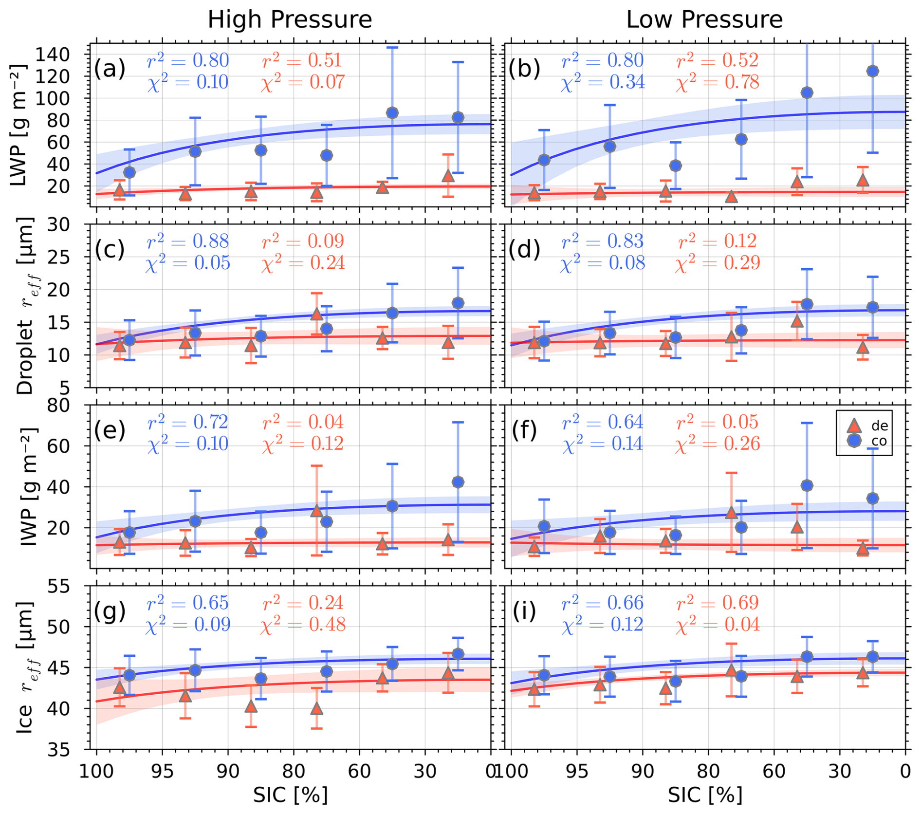
Figure 5 Cloud microphysical properties as a function of SIC (for SIC > 5 %) for coupled (blue circles) and decoupled (orange triangles) classes during the wintertime period from 2012 to 2024. H-/L-pressure systems are arranged on the left/right columns, respectively. Liquid water path (a, b); droplet effective radius (c, d); ice water path (e, f); ice effective radius (g, i). Symbols/bars represent the median$/\pm {\mathit{\sigma }}_{\text{mad}}$ for the distribution within SIC bins of every 20th percentile. Lines indicate the best fit with 95 % confidence interval (CI) shading around the solid lines. The r² and χ² are the best fit indicators for the model Eq. (3) for coupled/decoupled. Note that x-axis ticks and labels are not equidistant.

The results in Fig. 5 reveal that several microphysical cloud properties increase in magnitude as SIC decreases. The best-fitting empirical model is given by Eq. (3), which asymptotically approaches β₁ + β₂ as SIC → 0 %. This empirical model was specifically optimized for coupled cases; thus, poor fits for decoupled cases highlight differences between coupling regimes. For decoupled cases, only few cloud properties show a clear relationship with SIC, and many variables exhibit no significant correlation.

$$\begin{array}{}\text{(3)}& {\mathcal{F}}_{\mathrm{var}}(\text{sic};\mathit{\beta })={\mathit{\beta }}_{\mathrm{1}}+{\mathit{\beta }}_{\mathrm{2}}\exp \left({\text{sic}}^{\mathrm{2}}\right)\end{array}$$

where $\text{sic}\in \mathit{\{}\mathrm{0},\mathrm{\dots },\mathrm{1}\mathit{\}}$ is normalized sea ice concentration, ℱ_var is the observed cloud property (e.g. LWP, IWP, droplet r_eff, ice particle r_eff), and β₁, β₂ are empirically derived coefficients from non-linear curve fitting. Equation (3) was preferred over the power-law form ℱ = a SIC^b (PSG23) because the MOSAiC wintertime observations were predominantly above 90 % SIC, whereas this study spans SIC observations from 0 % to 100 % over 14 years, providing a more complete picture of cloud properties sensitive to SIC.

Specifically, Fig. 5 panels (a) and (b) reveal a clear increase in LWP with decreasing SIC in coupled cases (blue circles), levelling off at a median of ∼ 80 to 120 g m⁻² for SIC ≲ 30 %. When the observations are sorted according to weather system, the fit to Eq. (3) is better for H-pressure cases (r²=0.80 and χ²=0.1) than for L-pressure cases (r²=0.80 but χ²=0.34). For L-pressure, LWP exhibits higher variability, resulting in larger uncertainties in β₁ and β₂ in Eq. (3) (wider shaded CI in Fig. 5b), particularly due to outliers near 90 % SIC–80 % SIC. The decoupled LWP behaviour (orange triangles), align with Saavedra Garfias et al. (2023), confirming no significant relationship with SIC. This is supported by reduced r² of 0.51 (H-pressure) and 0.52 (L-pressure). Similarly, droplet effective radius (r_eff; Fig. 5c and d shows a strong negative correlation with SIC in coupled cases, but no significant relationship in decoupled cases.

Regarding IWP (Fig. 5e and f) no consistent change with SIC is observed in general. However, coupled cases show a strong positive correlation with decreasing SIC, particularly under H-pressure systems (r²=0.72). Decoupled cases show no statistically significant difference changes with SIC. These findings are consistent with pan-Arctic satellite observations by Cesana et al. (2024), who reported a negative correlation between SIC and ice cloud cover, and mixed-phase cloud cover, though differences in spatial and temporal scales exist.

For ice effective radius (Ice r_eff, Fig. 5g and i), a significant relationship with SIC is observed in coupled cases ($r^{\mathrm{2}}=\mathrm{0.65}/\mathrm{0.66}$ and ${\mathit{\chi }}^{\mathrm{2}}=\mathrm{0.09}/\mathrm{0.12}$ for H- and L-pressure cases), though the magnitude of change is smaller than for droplet r_eff. In decoupled cases, a similar trend is observed but with greater scatter, reducing r² to 0.24 for H-pressure systems. Notably, all MPC macro- and micro-physical properties are systematically lower in decoupled cases compares to their coupled counterparts.

Key MPC macrophysical properties are displayed in Fig. 6: Cloud geometrical depth (δ_h = CTH – CBH; Fig. 6a and b), liquid layer cloud base height (CBH; Fig. 6c and d), cloud top temperature (CTT; Fig. 6e and f), and cloud-layer temperature lapse-rate (Γ_cloud; Fig. 6g and i).

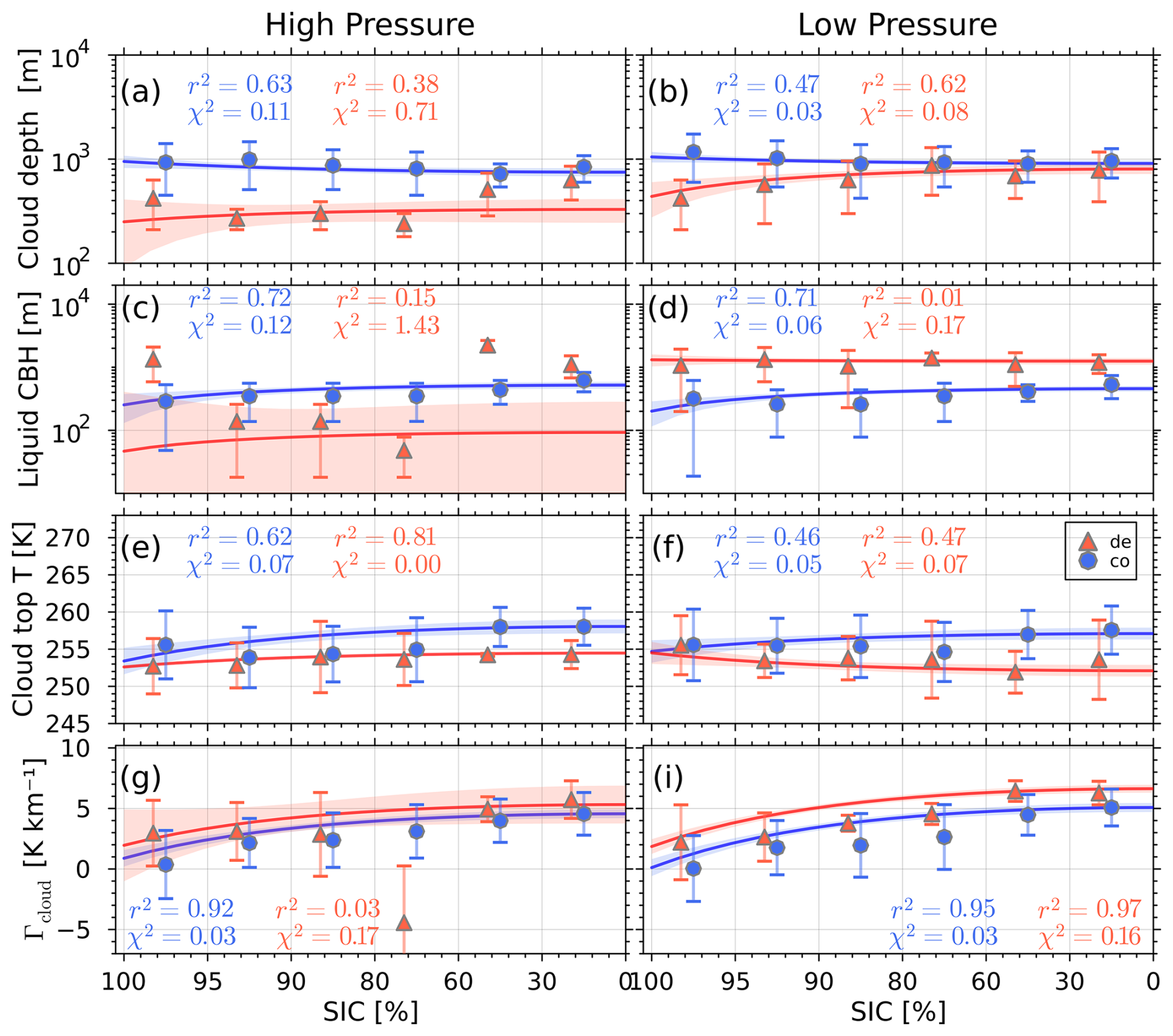
Figure 6 Same as Fig. 5 but for cloud depth (a, b); liquid layer cloud base height (c, d); cloud top temperature (e, f); cloud layer temperature lapse-rate (g, i). Symbols (bars) represent the distribution's median (± MAD) for SIC bin widths at every 20th percentile.

For decoupled MPC, no clear correlation with SIC is evident. This is reflected in low r² values (0.38 for δ_h, 0.15 for CBH) under H-pressure systems. In contrast, coupled cases show a clear decrease in δ_h with decreasing SIC (r²=0.63), indicating shallower clouds. These results confirm findings from the MOSAiC expedition: coupled MPC are generally thicker and have lower CBH than decoupled cases, independent of SIC – except for higher liquid CBH in coupled cases under H-pressure systems.

CTT (Fig. 6e and f) shows significant differences between coupled and decoupled cases, with a noticeable dependency on SIC: colder CTT for sea ice-covered ocean and warmer CTT over regions with open water. The model (Eq. 3) fits decoupled cases better (r²=0.81 and H-pressure) than coupled cases (r²=0.62). Coupled cases generally exhibit slightly higher CTT than decoupled cases.

The cloud-layer temperature lapse-rate (${\mathrm{\Gamma }}_{\mathrm{cloud}}=-{\sum }_{z=\mathrm{CBH}}^{\mathrm{CTH}}\left(\frac{T_{z+\mathrm{1}}-T_z}{H_{z+\mathrm{1}}-H_z}\right)$) is the only macrophysical property that showed pronounced modulation by SIC (Fig. 6g and i). Decoupled cases show systematically larger Γ_cloud values than coupled cases. The empirical model (Eq. 3) fits the data with a robust coefficient of determination of r²=0.95 and χ²=0.03 for the L-pressure and coupled cases. For H-pressure and L-pressure systems with SIC ≳ 95 %, the median Γ_cloud (blue dots in Fig. 6g and i SIC > 95 %) shows that approximately half of the distribution is negative – indicating a temperature inversion within the cloud layer (T_top>T_base). As SIC decreases (e.g. SIC < 95 %), Γ_cloud becomes clearly positive (i.e. T_top<T_base), indicating cooling with height and a tendency towards a moist adiabatic lapse-rate.

The results suggesting an apparent contradiction that shallower clouds with increasing LWP and IWP as SIC decreases, is resolved by the concurrent increase in liquid- and ice r_eff (Fig. 5c, d, g, i). Furthermore, surface air temperature (T2m) shows a positive correlation with several micro- and micro-physical properties, particularly in coupled cases. The physical explanation for the observed increase in LWP and IWP with the decrease of SIC (i.e. warmer surface) lies in enhanced latent and sensible heat fluxes from sea ice openings, which promote convection and sea salt aerosol release. When coupled to clouds, this drives increased cloud water content. These findings align with in-situ measurements in Svalbard, which suggesting that a warming Arctic enhances ice nucleating particles, enabling formation of ice-containing clouds at warmer temperatures (Tobo et al., 2024). Similarly, Schäfer et al. (2025) found in Arctic MPC simulations that a warming climate increases cloud ice water content via enhanced ice-nucleating particles and secondary ice production (e.g. rime splintering).

3.2 Year-to-year variability and trends

MPC properties are analysed as a time series across 14 years wintertime (WT) seasons $\mathrm{WT}=\mathit{\{}\mathrm{2011}/\mathrm{12},\mathrm{2012}/\mathrm{13},\mathrm{\dots },\mathrm{2024}/\mathrm{25}\mathit{\}}$, with each data point representing descriptive statistics (median, MAD) from observations within a given WT (e.g. “2012/13” = 1 November 2012 to 30 April 2013). No SIC-based separation is applied here.

A first attempt to analyse MPC time series observations at NSA site has been reported by Saavedra Garfias and Kalesse-Los (2024). They previously analysed a 10 year subset of coupled$/$decoupled MPC at NSA site, reporting the oscillatory nature of some MPC properties with time but no statistically significant trends using Ordinary Linear Regression (OLR). However, OLR is limited by two major shortcomings: i.e. heteroskedasticity (increased variance with higher median values) and residuals' bias with skewed distributions due to oscillatory signals – e.g. a local maximum LWP was found at 2016/17 between two local minima in 2013/2014 and 2018/2019 – violating OLR's assumption of normally distributed residuals.

To address these shortcomings, two robust methods are applied, both using weighted linear regression (WLR) with weights inversely proportional to the variance (Eq. A1) within wintertime (Chang et al., 2021):

• i.

  A 10 year running window smooths the time series (e.g. 2016/17 averaged over ±5 winters), then a weighted linear regression is applied. This reduces noise and mitigates heteroskedasticity.

• ii.

  The signal is modelled as following a natural cycle with a frequency occurring within the 14 years period. A fixed frequency ν_k [yr⁻¹] is applied to fit the data via non-linear regression following Eq. (4).

Both methods use weighted regression to account for varying cloud properties within a wintertime variability. The time series WLR fitting model to be applied for the methods i and ii are given by:

$$\mathcal{Y}(t;\mathit{\beta })\left\{\begin{array}{llr}{\mathit{\beta }}_{\mathrm{1}}& +{\mathit{\beta }}_{\mathrm{2}}t+\mathit{\epsilon }\mathrm{method}i.& \left(\mathrm{4}\mathrm{a}\right)\\ {\mathit{\beta }}_{\mathrm{1}}& +{\mathit{\beta }}_{\mathrm{2}}t+{\mathit{\beta }}_{\mathrm{3}}\cos \left(\mathrm{2}\mathit{\pi }{\mathit{\nu }}_{k}t-{\mathit{\beta }}_{\mathrm{4}}\right)& \\ & +\mathit{\epsilon }\mathrm{method}ii.& \left(\mathrm{4}\mathrm{b}\right)\end{array}\right.$$

where 𝒴(t;β) is the time dependent cloud parameter (e.g. LWP, IWP, cloud droplet/ice particle r_eff, etc.). In Eq. (4), t runs over the sequence of wintertime WT and the coefficient to fit is denoted by the vector $\mathit{\beta }=[{\mathit{\beta }}_{\mathrm{1}},{\mathit{\beta }}_{\mathrm{2}},\mathrm{\dots }]$, and ε represents the model residuals. In both Eq. (4a, b) the time series trend is determined from $\frac{\mathrm{\Delta }\mathcal{Y}}{\mathrm{\Delta }t}\equiv {\mathit{\beta }}_{\mathrm{2}}$. For Eq. (4b), ν_k represents the dominant frequency of the oscillating signal with phase shift β₄. Note that in Eq. (4b), ν_k is not determined by the regression but rather a so-called “free parameter”. ν_k is obtained from an external source; the selection of this free parameter is presented in detail later in Sect. 3.2.2.

The results are presented in Sect. 3.2.1 (method i) and Sect. 3.2.2 (method ii), followed by a comparative analysis.

3.2.1 Method i: Trend estimation using moving-average time series

After smoothing the MPC time series with 10 year moving average, data are fitted to Eq. (4a) using WLR. The trend is derived from the fitted coefficient β₂, and the results are sorted by the cloud coupling class and pressure system at NSA site.

Figure 7 depicts the time series of selected MPC properties that exhibit the largest variability along the years: LWP, liquid CBH and CTT. Coupled (blue circles), and decoupled (orange triangles) case are separated by pressure system. LWP exhibits strong inter-annual variability. Coupled LWP shows significant positive trends: $+\mathrm{4.4}\pm \mathrm{0.7}$ g m⁻² per decade under H-pressure and $+\mathrm{24.3}\pm \mathrm{0.7}$ g m⁻² per decade under L-pressure (Fig. 7a and b). Decoupled LWP remains lower overall and displays higher stochastic variability, resulting in a less pronounced and negative trend of $-\mathrm{5.3}\pm \mathrm{0.7}$ g m⁻² per decade under L-pressure.

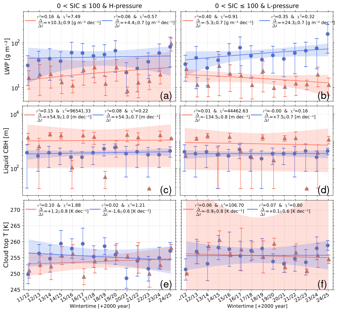
Figure 7 MPC time series for coupled (blue circles) and decoupled (orange triangles) represented by the median (${\mathit{\mu }}_{\mathrm{1}/\mathrm{2}}$) and σ_mad (bars) of wintertime distributions. H-pressure (left column) and L-pressure (right column) for LWP (a, b), liquid layer CBH (c, d), and cloud top temperature (e, f). The linear trends (± uncertainty) are indicated with the solid lines (shared area is 95 % confidence interval) and trend values in units per decade, the coefficient of determination r², and χ² are presented in legend.

Liquid layer CBH also shows clear trends (Fig. 7c and d). Under H-pressure, both coupled and decoupled CBH increase at similar rates ($+\mathrm{54.3}\pm \mathrm{0.7}$ and $+\mathrm{54.9}\pm \mathrm{1.0}$ m per decade, respectively). Under L-pressure, trends reverse: coupled CBH shows small change ($+\mathrm{7.5}\pm \mathrm{0.7}$ m per decade), while decoupled CBH decrease sharply ($-\mathrm{134.5}\pm \mathrm{0.8}$ m per decade).

CTT (Fig. 7e and f) shows no significant difference between coupled and decoupled cases, consistent with Sect. 3.1. In general, CTT median values slightly decrease over time, with the strongest reduction under H-pressure and coupled cases (trend: $-\mathrm{1.6}\pm \mathrm{0.6}$ K per decade), and the weakest (non-significant) trend under L-pressure and decoupled cases ($-\mathrm{0.9}\pm \mathrm{0.8}$ K per decade).

3.2.2 Method ii: Trends estimation considering cyclical time series

Given the oscillatory nature of MPC time series – first reported by Saavedra Garfias and Kalesse-Los (2024)–, we hypothesize that these oscillations are driven by intra-decadal climate variability. Climate teleconnections can influence Arctic sea ice formation/melting, thereby modulating MPC properties, as shown in Sect. 3.1. This suggest that observed MPC fluctuations may be linked to large-scale climate modes. The hypothesis is supported by two lines of evidence: Firsty, extensive literature confirms climate teleconnections between Tropical Pacific, sub-tropical regions and the Arctic (Timmermann et al., 2018; Kodaira et al., 2020; Zhang et al., 2023; Deng and Dai, 2024; Zhong et al., 2024); and secondly, MPC time series (e.g. LWP, CTT, δ_h, and CBH) exhibit patterns resembling ENSO or PDO cycles – e.g., LWP peaks align with strong El Niño events (positive ENSO in 2016 and 2023), and minima with La Niña events (negative ENSO in 2020 to 2022), with phase shift and amplitude differences across MPC variables.

To test this, we consider three major climate indices: Arctic Oscillation (AO), PDO, and ENSO. The free parameter ν_k (frequency of signal in Eq. 4b) is selected from relevant harmonics of these indices, identified via discrete Fourier analysis performed over the ENSO, PDO and AO signals (details in Appendix D). Only frequencies with Fourier amplitudes larger than 100 were considered (red triangles over the x-axis of Fig. D1c in Appendix D): ν_k={0.093, 0.155, 0.186, 0.217, 0.248, 0.279, 0.341, 0.434} yr⁻¹, corresponding to periods of {10.8, 6.5, 5.4, 4.6, 4.0, 3.6, 2.9, 2.3} yr – consistent with know climate modes e.g., 2.8, 4.3, and 5.7 yr for AO; 12 yr for ENSO; (Zhang and Moore, 2011). All ν_k values are common harmonics for ENSO, PDO and AO, though with varying levels of contributions. For each ν_k, the time series are fitted to Eq. (4b), and three goodness of fit metrics are calculated: χ², coefficient of determination r², and the normalized root mean square error nRMSE. The optimal ν_k is selected via a cost function (Eq. A5) minimizing χ² and nRMSE while maximizing r² (see Appendix A1 and Fig. A1 for example).

The time series of MPC properties fitted to Eq. (4b) to obtain the coefficients β are shown in Fig. 8 for H-pressure systems; L-pressure results are in Appendix Fig. B1. The best-fit frequency (ν_k in legend) and corresponding β coefficients (dashed lines in Fig. 8) represent the optimal model.

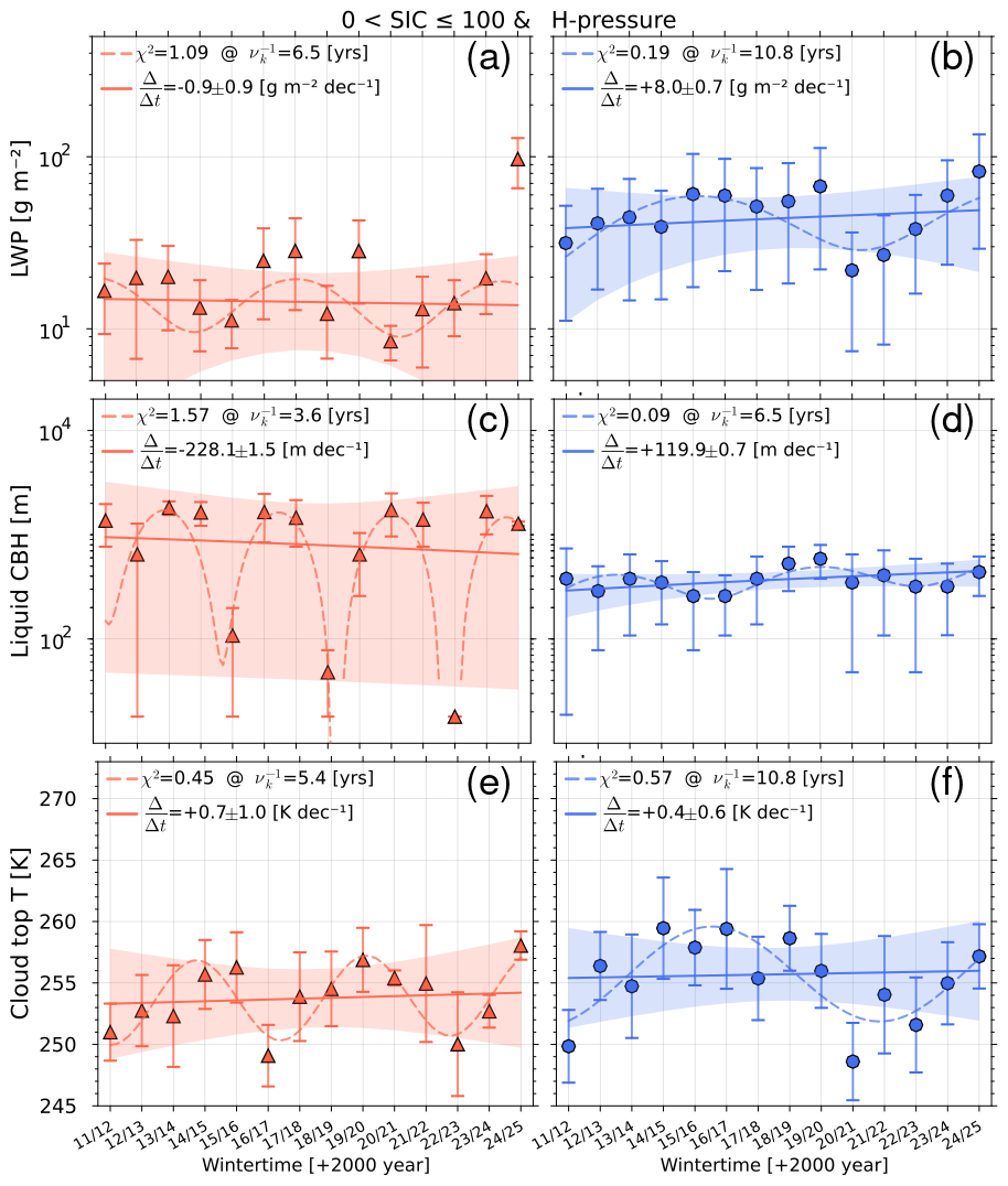
Figure 8 Same as in Fig. 7 but applying method ii for H-pressure systems. With LWP (a) and (b), liquid layer CBH (c, d), and CTT (e, f). Left column panels (a, c, e) show decoupled MPC (orange triangles) cases and right column (b, d, f) coupled MPC cases (blue circles). The best fit curves are dashed-lines and linear trends are the solid lines (shared area is 95 % CI). The goodness of fit coefficient χ², the period of the cyclical curve ${\mathit{\nu }}_k^{-\mathrm{1}}$, and trend values, in units per decade, are indicated in legend.

Under H-pressure systems:

• Decoupled LWP best fit by a 6.5 yr cycle (linked to AO/DPO), yielding a weak negative trend ($-\mathrm{0.9}\pm \mathrm{0.9}$ g m⁻² per decade).

• Coupled LWP follows a 10.8 year cycle (strongly tided to ENSO/PDO), with a significant positive trend ($+\mathrm{8.0}\pm \mathrm{0.7}$ g m⁻² per decade).

For liquid cloud base height (CBH; Fig. 8c and d):

• Decoupled CBH fits a 3.6 year cycle, with a trend of $-\mathrm{228.1}\pm \mathrm{1.5}$ m per decade.

• Coupled CBH fits a 6.5 year cycle, with a trend of $+\mathrm{119.9}\pm \mathrm{0.7}$ m per decade.

Cloud top temperature CTT (Fig. 8 e and f) shows slightly positive, non-significant trends (decoupled: $+\mathrm{0.7}\pm \mathrm{1.0}$ K per decade, and coupled: $+\mathrm{0.4}\pm \mathrm{0.6}$ K per decade)), best fit by 10.8 year (ENSO/PDO) and 5.4 year (ENSO) cycles, respectively. The 5.4 year cycle is the predominant intra-decadal ENSO signal and second strongest for PDO, but absent in AO (Appendix D).

3.2.3 Comparison of trends obtained by the two methods

Trends were estimated for all SIC > 0 %, and separately for the lower and upper 50th percentiles of SIC: SIC ∈ {(0, 95], (95, 100]} %. The notation (0, 95], indicates data with 0 % < SIC ≤ 95 %. Results are summarized in Fig. 9, where “All” refers to the full SIC range (Figs. 7 and 8).

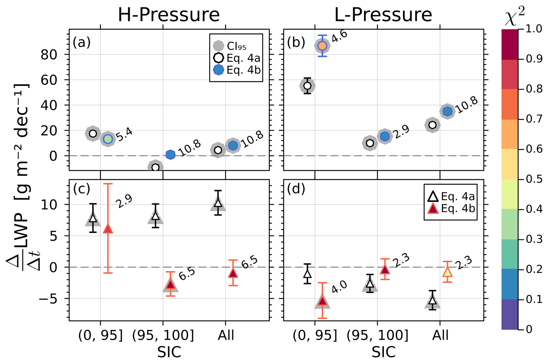
Figure 9 LWP trends for SIC subsets as indicated in the abscissae. The hollow symbols indicate the trend using method i (Eq. 4a), coloured symbols show results using method ii (Eq. 4b), grey shadows behind symbols indicate the trend is statistically significant (p<0.05), and the number next to the coloured symbols are the period in years for the best fit Eq. (4b). The colour bar represents the goodness of fit χ² value. MPC observed in the presence of H-pressure systems in panel (a) and (c) for coupled and decoupled cases, respectively. MPC in the presence of L-pressure systems in panels (b) and (d) for coupled (upper row) and decoupled (lower row) cases, respectively.

Coupled cases are shown in the top row Fig. 9a and b, decoupled in the bottom row (c and d). Hollow symbols represent method i (moving average WLR); coloured symbols denote method ii (harmonic fit), where the colour indicates χ² (the lower ≡ better fit). The period of best fit ${\mathit{\nu }}_k^{-\mathrm{1}}$ in Eq. (4b) is labeled next to each coloured symbol.

For coupled MPC-LWP, both methods agree well, especially under SIC > 95 %. For SIC < 95 %, discrepancies emerge: trends reach $\approx +\mathrm{55}$ (method i) and $\approx +\mathrm{86}$ g m⁻² per decade (method ii) under L-pressure in the lower 50th percentile SIC. Most coupled LWP trends align with PDO/ENSO periods (4.6, 5.4, and 10.8 years).

In contrast, decoupled MPC-LWP shows high variability. Under H-pressure, method ii reveals a reversal in trend sign with increasing SIC – positive at low SIC, negative at high SIC. Under L-pressure, both methods yield slightly negative trends (Fig. 9d). Oscillations are dominated by AO and ENSO (i.e. 2.3, 2.9, 4.0, 6.5 years), with shorter periods than for coupled cases.

For ice properties, IWP in coupled clouds shows no significant trend under L-pressure (method i), nor does ice effective radius (r_eff; Fig. S2b, c, d). However, method ii reveals a significant positive IWP trend under L-pressure (2.9 years ENSO cycle, Fig. S5b) and H-pressure (10.8 years ENSO/PDO cycle, (Fig. S4b). This suggests that cloud responses are driven by weather patterns and warm-air intrusions from lower latitudes – consistent with finding by Cesana et al. (2024) in the Bearing Sea using satellite observations.

4 Conclusions

The main objective of this study is to extend and validate our understanding of the physical link between Arctic sea ice conditions and mixed-phase cloud (MPC) properties – originally established for data obtained at the MOSAiC expedition in the Central Arctic – to 14 years of multi-sensor observations from the ARM North Slope of Alaska (NSA) site in the Western Arctic. This is achieved by two approaches: first, by applying the PSG23 method developed for wintertime observations during MOSAiC to multi-year observations at the NSA site (in Sect. 3.1); and second, by performing a multi-year time series analysis of the MPC properties (Sect. 3.2). In the following, results are set into context with the MOSAiC expedition, and the long-term time series analysis.

On the MPC properties modulated as a function of SIC, coupling status, and pressure system

Section 3.1 along with Figs. 5 and 6 are only partially comparable to the findings reported by PSG23 for the MOSAiC expedition. This is because the MOSAiC study mainly relies on the sea ice lead fraction (LF) to represent the sea ice states. For the present study, long-term and continues LF data are not available. Furthermore, SIC MOSAiC winter was above 90 %, in contrast to NSA site observations during the 14 years where a larger variation in SIC was covered. Keeping these caveats in mind, the following phenomena reported by Saavedra Garfias et al. (2023) can be confirmed:

• LWP of coupled clouds increases as the sea ice states trend to larger openings, whereas LWP of decoupled clouds has no relationship with SIC. The present study confirms MOSAiC findings and extends its validity for SIC as low as 5 %.

• Cloud layers for coupled cases are thicker and have a lower liquid layer base height than the decoupled cases.

• For coupled cases with SIC > 95 %, cloud layer temperature lapse-rate (Γ_cloud) ranges from negative to positive values, whereas decoupled cases show a distribution predominantly above zero. For SIC < 95 %, Γ_cloud increases with increasing sea ice opening, regardless of coupling status.

Conversely, new findings that the study from the MOSAiC expedition did not conclude can be summarized as follows:

• Under L-pressure systems and for all SIC, coupled clouds have a lower liquid cloud base height than decoupled clouds. This difference is only evident for H-pressure systems when SIC ≳ 95 %.

• A negative relationship between IWP and SIC was found, albeit only for coupled MPC.

• The liquid and ice effective radii (r_eff), which Saavedra Garfias et al. (2023) reported for MOSAiC showed no clear difference when sorted by coupling status or lead fraction, were found to exhibit a strong dependence on SIC in coupled cases. Specifically, r_eff increased with decreasing SIC.

• For coupled MPC, a negative Γ_cloud (in-cloud temperature inversion) is possible at SIC > 95 %. At lower SIC, Γ_cloud>0 shows a tendency toward a moist adiabatic lapse-rate. Decoupled cases consistently exhibit a moist adiabatic lapse-rate, with increasing magnitude as SIC decreases-particularly under L-pressure systems.

On the long-term trends of MPC properties

Two trend estimation methodologies highlight method-dependent biases. Method i, a standard approach for stochastic periodic signals, is sensitive to edge effects and moving window width. Disagreements arise, particularly in L-pressure decoupled LWP trends: method i shows a decline of $-\mathrm{5.3}\pm \mathrm{0.7}$ g m⁻² per decade, while method ii indicates a slight increase of $+\mathrm{0.9}\pm \mathrm{0.9}$ g m⁻² per decade. This discrepancy stems from Method i's fixed window size, which over-smooth the data, whereas method ii captures a dominant 6.5 years cycle -shorter than the 10 years window- leading to more accurate trend representation.

Disagreement also occurs for the liquid cloud base height of decoupled MPC. Method i detects a trend of $+\mathrm{54.9}\pm \mathrm{1.0}$ m per decade, while method ii reveals a negative trend of $-\mathrm{228.1}\pm \mathrm{1.5}$ m per decade – both statistically significant. Figure 8c shows how method ii captures a periodic signal of ∼3.6 years, which better fits the low CBH values observed during negative ENSO phases (e.g. 2018/19, 2022/23), whereas method i effectively suppresses these short-term variations.

Both methods agree on IWP trends under H-pressure, showing coupled case trends of $+\mathrm{3.5}\pm \mathrm{0.8}$ g m⁻² per decade (method i) and $+\mathrm{4.4}\pm \mathrm{1.0}$ g m⁻² per decade (method ii) with a 10.8 year period characteristic for ENSO and PDO (Sect. S2.2).

Based on time series of surface skin temperature as indicator of coupled clouds radiative feedback, we found that a continuing warming in the Western Arctic can only be attributed to L-pressure systems associated with observations under SIC < 95 %. In contrast, under H-pressure systems and SIC ≥ 95 %, our results show a decrease in cloud radiative-induced surface temperature.

Hypothesizing the influence of climate modes on MPC variability, we fit the data to Eq. (4b) with one relevant harmonic as a free parameter ν_k. The NSA site time series are best explained by ENSO's 5.4 and 10.8 years, PDO's 6.5 and 10.8 years, and AO's 2.3 and 2.9 year periods. ENSO and PDO (10.8, 5.4 year) dominate most MPC parameters, with AO (2.3, 2.9 year) and PDO (6.5 year) as secondary contributions. Decoupled MPC under H-pressure varies on intermediate periods (3.6, 4.0, 5.4 years), while coupled MPC shows longer cycles (6.5, 10.8 years). Under L-pressure, decoupled MPC oscillates at 2.3 to 6.5 years, and coupled MPC at 2.9, and 10.8 years, depending on the specific MPC property.

Discussion

The MOSAiC's derived distinction between coupled and decoupled MPCs, based on water vapour transport-sea ice interaction, is confirmed at the NSA site. The multi-year NSA dataset further enabled the assessment of the influence of atmospheric pressure systems. Results show that MPC properties depend not only on coupling status but also on the prevailing weather pressure system. Under L-pressure systems, coupled LWP, cloud top temperature, and liquid layer base height exhibit positive long-term trends. In contrast, decoupled cases show no significant trend in LWP or CTT, while liquid layer base height was found to decrease. Under H-pressure systems, similar directional trends are observed, albeit with differing magnitudes.

A limitation of this study is that the current remote sensing capabilities at the NSA site do not provide vertical distribution of aerosols, which hinders the investigation of marine aerosol effects on LWP and IWP in conjunction to SIC changes. Moreover, only the local atmospheric pressure has been used to assess the relevant pressure system for NSA site, which does not necessary represent meso-scale synoptic weather pattern for the western Arctic.

This study uses empirical mathematical models derived from long-term observations to parameterize atmospheric boundary layer MPC ascribed to Arctic sea ice conditions; revealing that MPC properties are strongly modulated by sea ice concentration, cloud coupling status, atmospheric pressure systems, and intra-decadal climate variability – providing critical constraints for improving cloud and climate model representation. We argue that MPC in Arctic climate models need to capture the complexity revealed here – beyond small-scale horizontal moist air mass transport linking sea ice leads to downstream clouds – by incorporating weather patterns, large-scale circulation, intra- and multi-decadal climate oscillations, and Arctic-lower latitude teleconnections. Recent studies highlight the implications of this complexity for decadal climate predictability (Timmermann et al., 2018; Mann et al., 2020; Cesana et al., 2025), with similar findings reported by Lubin et al. (2026), who linked long-term LWP and CRE (1999–2024) to large-scale circulation and atmospheric rivers. Our findings are aligned with those studies providing a robust observational verification, underscoring the critical role of sustained, long-term high-quality Arctic monitoring networks like the ARM NSA site for enabling such insights.

Appendix A: Statistical parameters used in the data analysis

The statistics for cloud properties are represented by the geometric mean, median or 1st and 3rd quantile. The variability within the distribution is expressed by the standard deviation (σ_g) or MAD (σ_mad). When the data mean or median is used to fit an analytical model, the variability within the distribution is taken into account by performing a weighted fitting either by linear or non-linear regression. The weights are modelled as

$$\begin{array}{}\text{(A1)}& {\mathit{\omega }}_j={\displaystyle \frac{{\mathit{\sigma }}_j^{-\mathrm{2}}}{\langle {\mathit{\sigma }}_j^{-\mathrm{2}}\rangle }}\end{array}$$

with ${\mathit{\sigma }}_j^{-\mathrm{2}}$ is the inverse of the variance (with σ_j can be σ_g or σ_mad), and $\langle {\mathit{\sigma }}_j^{-\mathrm{2}}\rangle =\frac{\mathrm{1}}{N}\sum _j{\mathit{\sigma }}_j^{-\mathrm{2}}$ is the inverse variance mean. The index j represents a distribution of cloud properties, which for the case of Sect. 3.1 $j\in \mathrm{SIC}=\mathit{\{}\mathrm{10},\mathrm{20},\mathrm{\dots },\mathrm{100}\mathit{\}}$ is the distribution within binned sea ice concentration, and for the case of Sect. 3.2 $j\in \mathrm{WT}=\mathit{\{}\mathrm{2011}/\mathrm{12},\mathrm{\dots },\mathrm{2024}/\mathrm{25}\mathit{\}}$ for the wintertime. In both cases N is the length of j set. The Eq. (A1) penalize large variability within the distribution j and will influence less the fitting algorithm.

A1 Model Goodness of fit test

To quantify the degree of a fitted model can represent the observations, the following parameters for goodness of fit are used:

• χ²: is the sum over residuals square divided by the fitting model degrees of freedom ν, which indicates how close the model prediction is from the data,

  $$\begin{array}{}\text{(A2)}& {\mathit{\chi }}^{\mathrm{2}}={\displaystyle \frac{\mathrm{1}}{\mathit{\nu }}}\sum _{j=\mathrm{1}}^N{\left({\displaystyle \frac{{\mathit{\epsilon }}_j}{{\mathit{\sigma }}_j}}\right)}^{\mathrm{2}}\end{array}$$

  where $\mathit{\epsilon }=\widehat{y_j}-y_j$ are the residuals (difference between model prediction $\widehat{y_j}$ and observed value y_j) in Eqs. (3) and (4a, b); with ν=2, 2, and 4, respectively. The closer χ² is to zero, the better the fir curve represent the data.

• r²: is the coefficient of determination, which quantifies how good the model explains the change in observed value,

  $$\begin{array}{}\text{(A3)}& r^{\mathrm{2}}=\mathrm{1}-{\displaystyle \frac{\sum _j{\mathit{\epsilon }}_j^{\mathrm{2}}}{\sum _j{\left(〈y_j〉-y_j\right)}^{\mathrm{2}}}}\end{array}$$

  where 〈y_j〉 is the average over all observed values y_j. Worth to note that r² is generally a valid parameter for linear relationships, while for non-linear regression it could produce unexpected results like negative values or larger than one (Spiess and Neumeyer, 2010).

• nRMSE: is the normalized root mean square error, which is the overall mean squared residual between model fitted and observed value,

  $$\begin{array}{}\text{(A4)}& n\text{RMSE}={\displaystyle \frac{\sqrt{\frac{\mathrm{1}}{N}\sum _j\left({\mathit{\omega }}_j^{\mathrm{2}}{\mathit{\epsilon }}_j^{\mathrm{2}}\right)}}{\text{IQR}}}\end{array}$$

  with IQR is the distribution inter-quantile region, and ω_j the weights as in Eq. (A1). Values of nRMSE larger than one signalize a very poor agreement between fitted model and observations.

Given a set of fitted parameters to Eq. (4b) corresponding to the six ν_k values, a goodness of fit test is performed to determine which single ν_k represents the data the best. This is done by minimizing a cost function which is dependent of all three goodness of fit parameter χ², nRMSE, and the reciprocal of r² i.e. 1−r², thus all three parameters range from zero (best) to higher values (worst):

$$\begin{array}{}\text{(A5)}& \mathcal{L}=\sqrt{{\mathit{\chi }}^{\mathrm{2}}+n{\text{RMSE}}^{\mathrm{2}}+(\mathrm{1}-r^{\mathrm{2}})}\end{array}$$

As an example of how the minimum is found, in Fig. A1 can be seen the cost function for two MPC parameters: LWP and CTT, with the minimum of the cost function ℒ indicated by the vertical thick line.

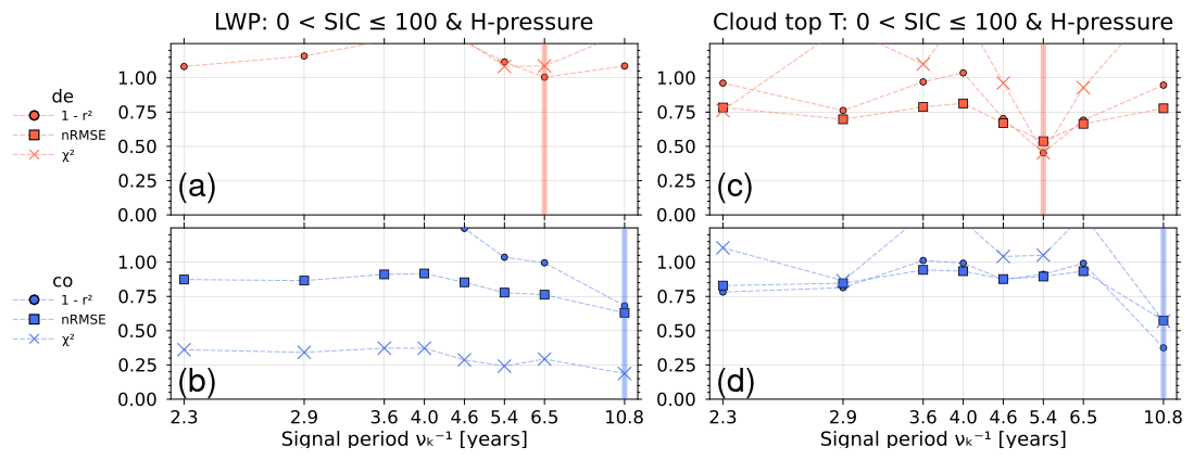
Figure A1 Determination of the best ν_k value, from the combination of all three goodness of fit parameters. LWP coupled (a) and decoupled (b), cloud top temperature coupled (c) and decoupled (d). The χ² is shown as crosses, nRMSE as squares, and the reciprocal of r² as circles. The thick vertical line is the value of ν_k that minimizes the cost function ℒ.

Appendix B: Results for trend estimation

To complement Sect. 3.2.2, the equivalent of Fig. 8 but for L-pressure systems is shown in Fig. B1 with LWP in panels (a) and (b), liquid CBH in panels (c) and (d), and cloud top temperature in panels (e) and (f). Further results of time series trends of other MPC properties can be found in the Supplement.

Figure B1 Same as in Sect. 3.2.2, Fig. 8 but for time series comprised of L-pressure systems.

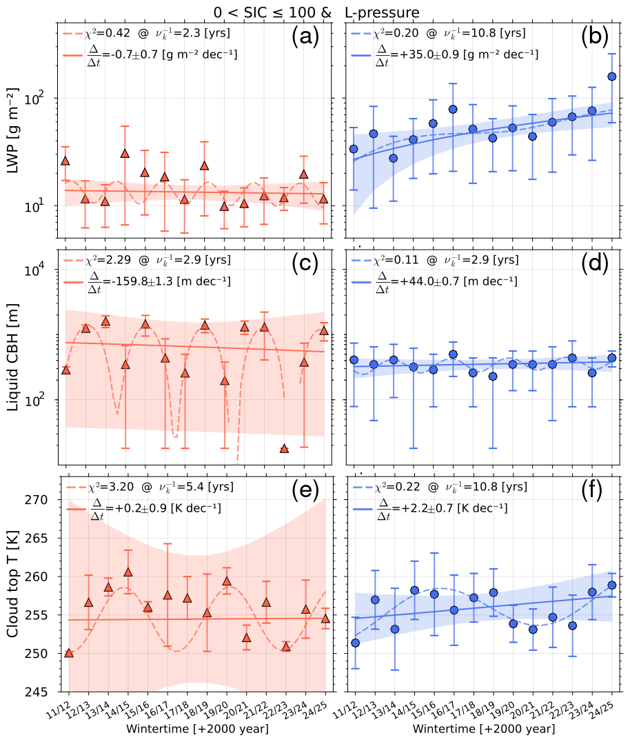
B1 Time series for the lower/upper 50th percentile SIC decomposition

The time series' trend analysed by method ii are decomposed by the lower and upper 50th percentile of sea ice concentration. For the period of 14 years observations the lower 50th percentile comprises of data with SIC between 0 % and 95 %, whereas the upper half from SIC above 95 % to 100 %. Figure B2 shows the LWP SIC decomposition.

B2 Surface skin temperature trend results after SIC decomposition

Time series analysis for the surface skin temperature T_skin, estimated from the net down- and up-welling longwave radiation flux (Saavedra Garfias et al., 2024), or by down-welling infrared radiometer when the former data is not available, after being decomposed in SIC subsets of 50th percentiles (shown in Sect. S2.3, Fig. S8) applied to methods in Sect. 3.2.1 and 3.2.2 are displayed in Fig. B3. These results are discussed in Sect. 3 in relation to the warming in the western Arctic.

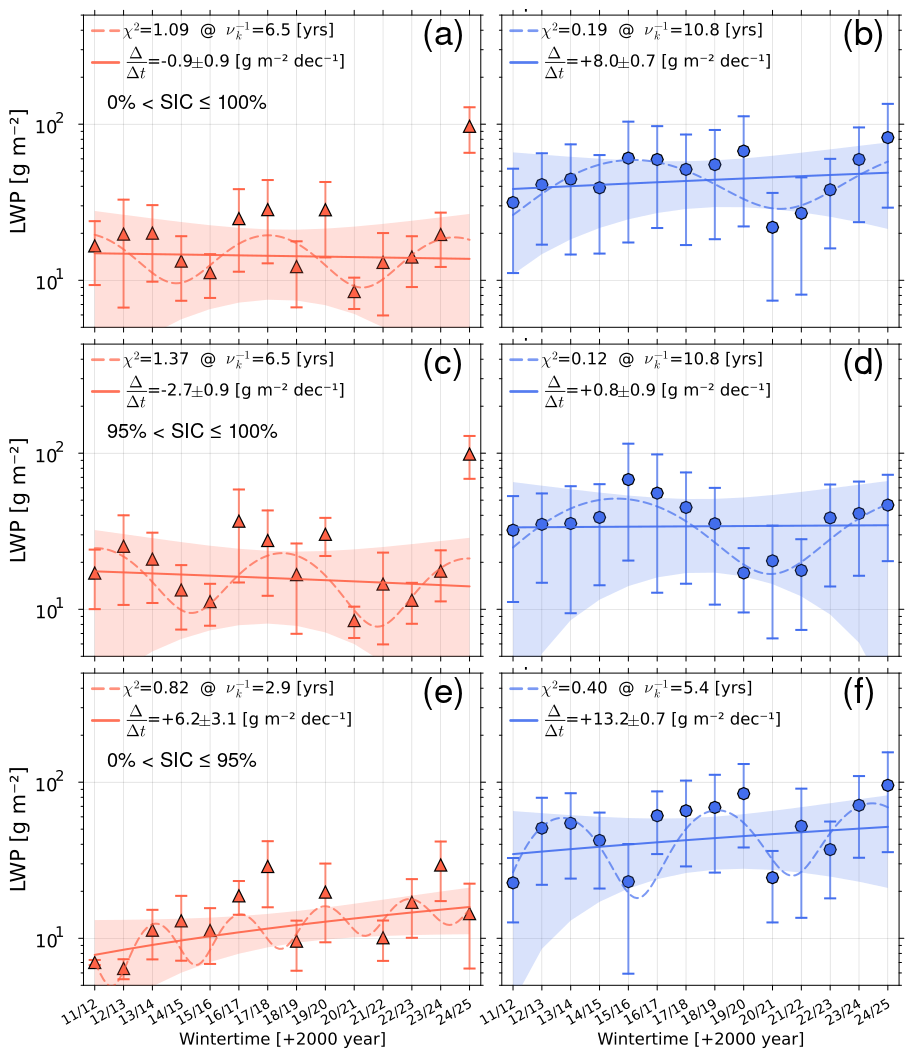
Figure B2 Time series of LWP for coupled and decoupled clouds under H-pressure systems. The time series are decomposed by the range of SIC: (a) and (b) all SIC considered, (c) and (d) for SIC > 95 % and SIC ≤ 100 %, and (e) and (f) for SIC > 0 % and SIC ≤ 95 %.

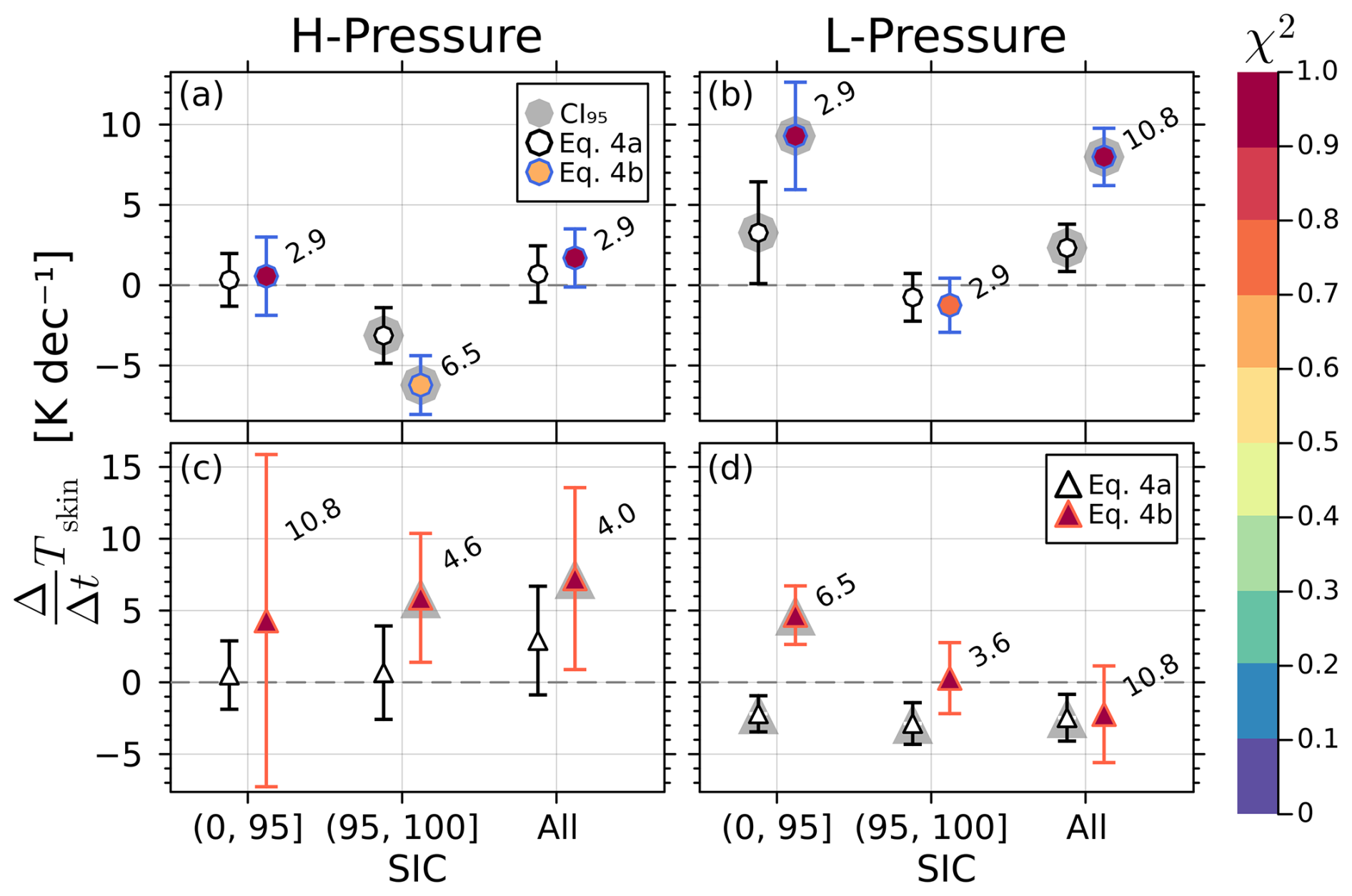
Figure B3 T_skin rate of change for SIC subsets in the abscissae. The hollow symbols are trends using method i (Eq. 4a), coloured symbols use method ii (Eq. 4b), grey shadows behind symbols indicate the trend is statistically significant (p<0.05), and the number next to the coloured symbols is the period in years for the best fit Eq. (4b). The colour table represents the goodness of fit χ² value. H-pressure systems in panel (a) and (c) for coupled and decoupled cases. L-pressure systems in panels (b) and (d) for coupled and decoupled, respectively.

Appendix C: Sensitivity to radius of semi-circle around NSA site for SIC parameter

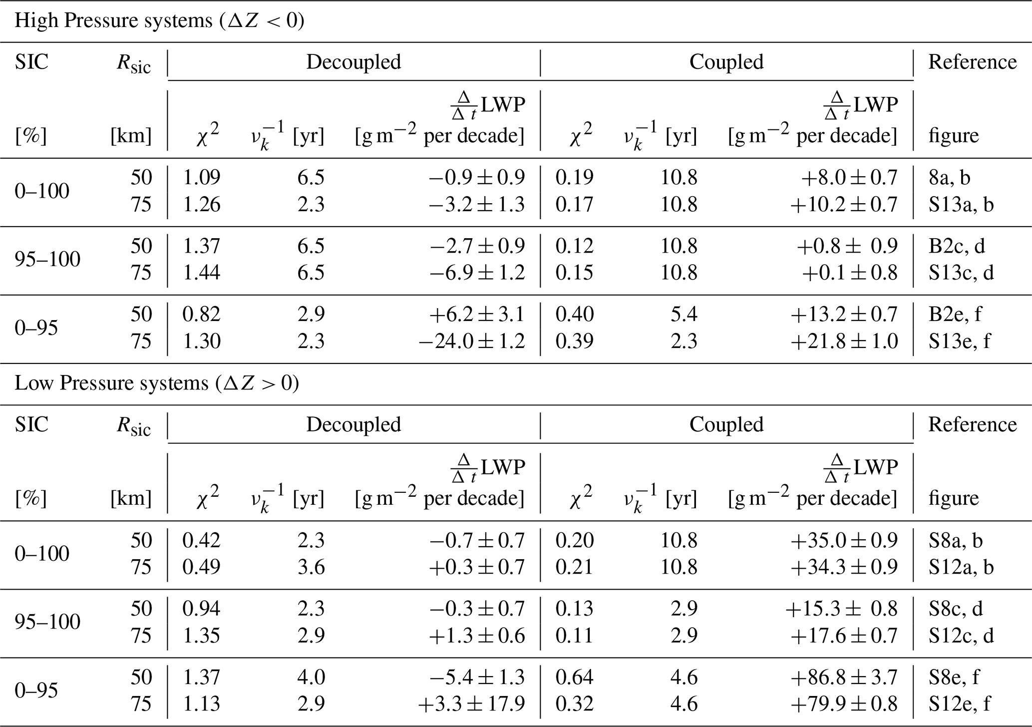
To investigate how sensitive the results are to the choice of sea ice area (red cone in Fig. 1) to compute the average SIC associated to be coupled/decoupled to the MPC parameters, in addition to the 50 km used for the results in Sect. 3, a different radius of 75 km has been tested. The procedure indicated in Sect. 2 was repeated for 75 km and the results for LWP trend are summarized in Table C1 as compared to the results for 50 km. It has been found that there is a small difference between results from 50 and 75 km radius (second column in Table C1), but the differences are more noticeable for decoupled cases in particular when grouped to 0 ≤ SIC < 95 %.

In Sect. S3 the associated Figure for 75 km radius around NSA site can be found. A noticeable difference is mostly seen for the results associated to decoupled cases and SIC between 0 % and 95 %. For coupled cases the results are robust and consistent either by selecting SIC within 50 or 75 km.

Table C1 Comparison for 2011 to 2024 wintertime LWP trends when considering SIC within two sectors of radius 50 or 75 km.

Appendix D: Frequency decomposition for climate indicators

A discrete Fourier analysis has been performed to obtain the frequency harmonics ν_k from three climate indicators: Arctic oscillation (AO), Pacific Decadal Oscillation (PDO), and El Niño Southern Oscillation (ENSO). The power spectrum as a function of the signal harmonics expressed as periods (${\mathit{\nu }}_k^{-\mathrm{1}}$) is shown in Fig. D1, with the set of harmonics used to test the fitting of Eq. (4b) indicated by a red triangle at the bottom of panel (c) in Fig. D1.

Note that the limits of the abscess in Fig. D1 is intentionally cut for the range relevant to the 12 year of observation period, the signal can contain multi-decadal harmonics that excesses the 12 years period.

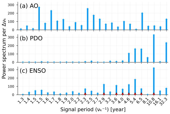
Figure D1 Power spectrum per frequency bandwidth for three climate indicators: (a) Arctic Oscillation, (b) Pacific Decadal Oscillation, (c) El Niño Southern Oscillation. The relevant frequencies are indicated by red triangles at the bottom of panel (c). Note, the peak at 10.5 year in panel (b) is cut at 300 for comparison reasons.

Appendix E: List of Acronyms and variables

Acronym	Description
AMSR2	Advanced Microwave Scanning
	Radiometer 2
AO	Arctic Oscillation
ASI	Arctic sea ice algorithm
CEIL10m	Ceilometer 10 m resolution
CRE	Cloud Radiative Effect
ENSO	El Niño Southern Oscillation
INTERPSONDE	Interpolated Radiosonde
KAZR	Ka Zenith Radar
MPC	Mixed-phase Clouds
NSA	North Slope of Alaska
MWR	Microwave Radiometer
PDO	Pacific Decadal Oscillation

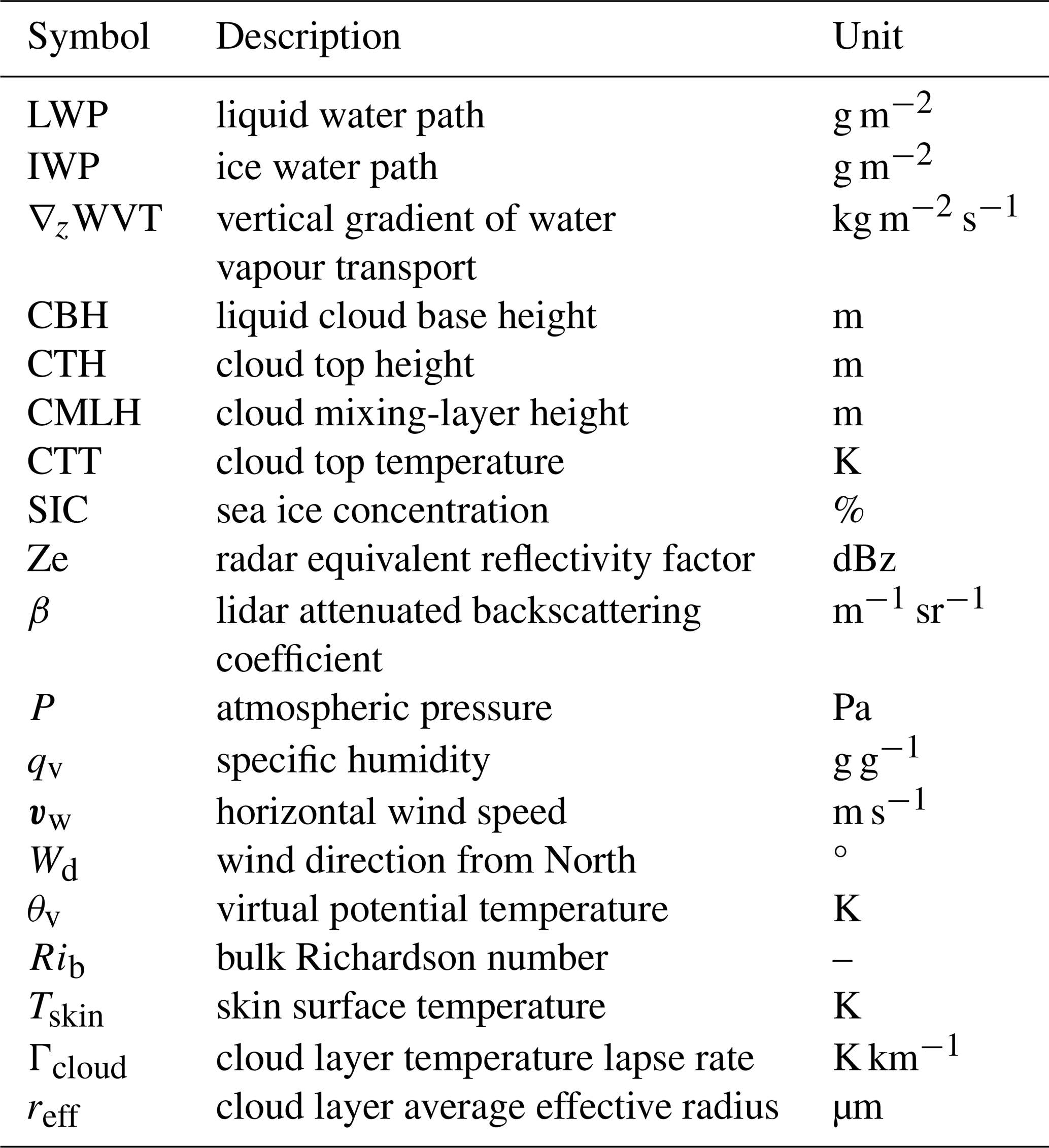
Table E1 Physical quantities and corresponding units relevant in this study.