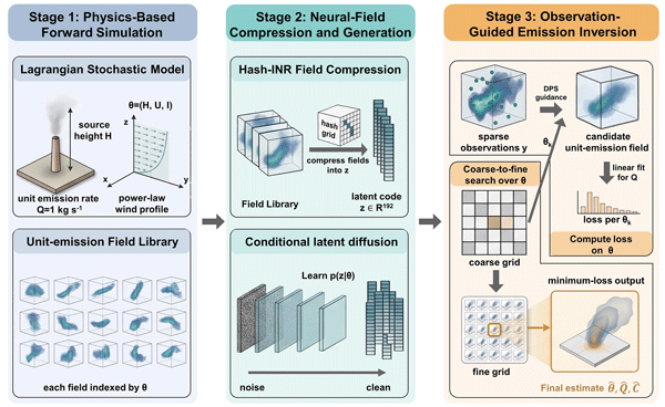
NeuPlume: generative inversion of atmospheric point-source emissions from sparse observations

Inverting point-source emissions from sparse atmospheric observations is difficult because emission rate, release height, wind speed, turbulence, and plume morphology can compensate for one another. We present NeuPlume, a neural-physical framework that formulates inversion as observation-guided generation and selection of complete three-dimensional concentration fields. A Lagrangian stochastic model builds a scenario-specific forward library, a conditional neural field compresses the simulated fields, and a latent diffusion model learns their conditional distribution. During inversion, diffusion posterior sampling generates candidate fields on a coarse-to-fine parameter grid, and NeuPlume returns the parameters and field that best match the observations. Across 30 synthetic cases, the selected fields achieve a mean spatial correlation of 0.942 and a mean emission-rate error of 13.6 %. Matched stress tests show that both observation geometry and transport-model fidelity govern inversion quality: trajectory-concentrated sampling weakens full-field reconstruction, while unrepresented transport alters parameter identification and, for effective plume rise, also degrades field reconstruction. Applied to four UAV methane transects above a coal-mine ventilation shaft, NeuPlume yields known-U minimum-loss emission estimates of 5.27–15.85 kt yr⁻¹ and exposes wind-speed and height-boundary sensitivities under model mismatch. NeuPlume thus provides an extensible methodology for jointly estimating source parameters and concentration fields: additional transport regimes can be incorporated through regime-specific simulation ensembles and neural-model retraining.

1 Introduction

Quantifying greenhouse-gas emissions from individual point sources supports emission inventories, regulatory assessment, and verification of mitigation commitments. Gaussian plume (GP) models estimate emission rate by fitting analytical dispersion kernels to downwind concentration measurements (Shah et al., 2019). Mass-balance (MB) methods integrate tracer flux across one or more cross-wind planes (Conley et al., 2017; Varon et al., 2018). Both approaches are used with ground, airborne, satellite, and unmanned aerial vehicle (UAV) observations (Shaw et al., 2021).

Sparse near-field measurements challenge these methods because source parameters, meteorology, observation geometry, and plume morphology remain coupled. GP methods commonly assume steady conditions, a spatially homogeneous wind field, and Gaussian cross-wind and vertical profiles. Near-field turbulence and plume meandering produce non-Gaussian structures (Yuvaraj et al., 2026), while rapidly varying winds violate the steady-state assumption (Jia et al., 2025). MB methods avoid prescribing a Gaussian plume shape but remain sensitive to incomplete plume interception, background subtraction, and the wind speed used to convert concentration into flux. UAV and controlled-release experiments show that observation coverage, cross-section geometry, and wind inputs substantially affect methane quantification (Mohammadloo et al., 2025; Liu et al., 2024).

Wind-speed representativeness is especially important because source strength and effective advective speed are coupled in steady passive-tracer transport. In an AVIRIS-4 campaign, wind-speed uncertainty contributed up to 99.4 % of the variance in cross-sectional-flux methane inversion (Meier et al., 2026). Controlled-release experiments using sequential airborne imagery found that ERA5 winds underestimated effective plume transport velocity by approximately 28 % (Eastwood et al., 2025). Airborne methane detection and coal-mine remote-sensing studies likewise identify wind information as a major source of emission-quantification error (Conrad et al., 2023; He et al., 2024). Jointly searching wind speed with source parameters provides a direct diagnostic of this coupling, although sparse observations may leave several parameter combinations with similar mismatch.

Bayesian inversion provides one established treatment of non-uniqueness by combining a parameter prior and an observational likelihood. Markov chain Monte Carlo (Xu et al., 2025), variational data assimilation (Aghdasi et al., 2025), regional-network inversion (White et al., 2019), and ensemble source reconstruction (De Meutter et al., 2021) have all been applied to atmospheric source estimation; recent reviews compare these methods with optimization-based alternatives (Xie et al., 2026). Their computational cost grows with parameter dimension and state complexity, particularly when source terms, meteorological parameters, and spatial concentration fields are inferred jointly.

Deep generative models offer a complementary route by learning low-dimensional representations from physical simulations and using measurements to guide candidate generation. Conditional diffusion models have been used for inverse reconstruction of permeability and seismic wavefields (Liu et al., 2025b; Meng et al., 2024). Conditional neural field (CNF) latent diffusion frameworks combine field compression with diffusion posterior sampling (DPS) to reconstruct turbulent fields from incomplete observations (Du et al., 2024; Liu et al., 2025a). In atmospheric point-source applications, learned plume representations can preserve non-Gaussian structure that analytical plume models omit. Zhao et al. (2026), for example, combined a U-Net encoder with inverse Gaussian fitting to reduce UAV emission-rate error.

This paper presents NeuPlume, a three-stage generative inversion framework for atmospheric point-source emissions. First, a Lagrangian stochastic model generates a library of concentration fields indexed by source and meteorological parameters. Second, a CNF compresses each field into a latent representation, and a denoising diffusion probabilistic model learns the conditional distribution of those representations. Third, NeuPlume runs observation-guided DPS on a coarse-to-fine parameter grid, estimates the emission rate at each node, and returns the candidate with the lowest observation mismatch. The main contributions are:

1. We formulate near-field source estimation as generative candidate-field inversion, jointly returning a minimum-loss parameter vector and its complete three-dimensional concentration field.

2. We define a simulator-independent implementation path in which a forward model maps scenario parameters to the concentration-field library used to train a new CNF and diffusion model.

3. We evaluate minimum-loss parameter and field accuracy on 30 held-out synthetic cases and use six representative off-grid cases within the trained parameter support for controlled baseline and component comparisons.

4. We apply the framework to public UAV methane observations above a coal-mine ventilation shaft and use matched stress tests to quantify sensitivity to observation geometry and unrepresented transport mechanisms.

2 Methods

2.1 NeuPlume model architecture

NeuPlume learns plume morphologies from forward simulations and uses sparse measurements to guide the generation and selection of candidate concentration fields.

The framework has three stages (Fig. 1). Stage 1 uses a Lagrangian stochastic model (LSM) to generate concentration fields at a unit emission rate $Q=\mathrm{1}\mathrm{kg}{\mathrm{s}}^{-\mathrm{1}}$. Each field is indexed by $\mathit{\theta }=(H,U,I)$, where H is effective release height, U reference wind speed, and I turbulence intensity. Stage 2 uses Hash-INR to compress each field into a 192-dimensional latent code z, and a denoising diffusion probabilistic model (DDPM) learns p(z∣θ). In Stage 3, sparse observations guide diffusion posterior sampling (DPS) at each candidate θ_k. NeuPlume decodes a candidate unit-emission field, fits Q by linear scaling, evaluates the observation mismatch, refines the search around the lowest-loss coarse-grid node, and returns $(\widehat{\mathit{\theta }},\widehat{Q},\widehat{C})$ from the minimum-loss fine-grid candidate.

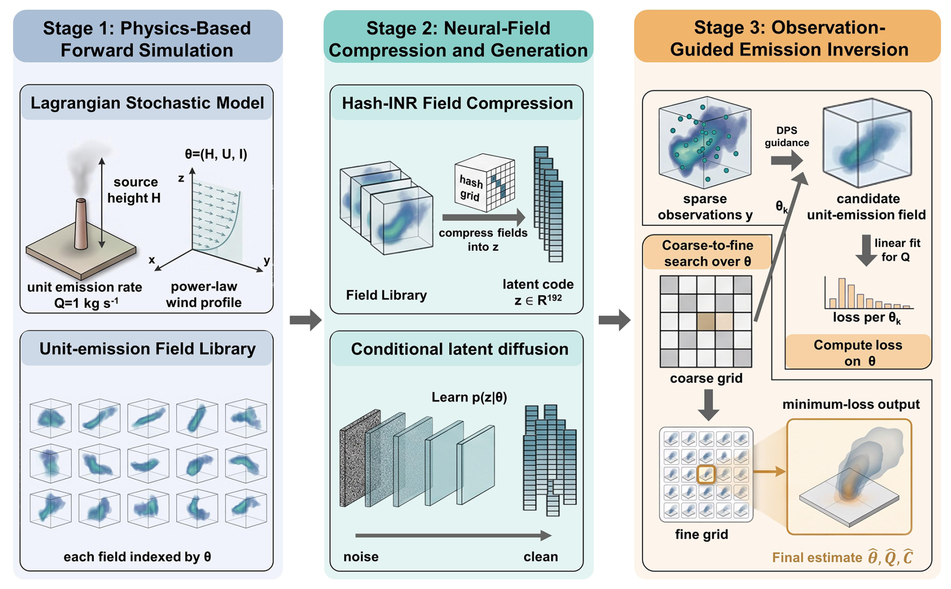
Figure 1 Overview of the three-stage NeuPlume framework. Stage 1 constructs a unit-emission field library with a Lagrangian stochastic model. Stage 2 compresses the fields with Hash-INR and learns their conditional latent distribution. Stage 3 combines observation-guided diffusion posterior sampling with coarse-to-fine parameter search and emission-rate fitting to obtain the minimum-loss reconstruction.

Let C(x∣θ) denote a unit-emission concentration field and let ℋ map the complete field to the measurement locations. The observations satisfy

$$\begin{array}{}\text{(1)}& {\displaystyle }{\displaystyle }\mathit{y}=Q\mathcal{H}\left[C(\mathit{x}\mid \mathit{\theta })\right]+\mathit{ϵ},\end{array}$$

where ϵ collects measurement and representation residuals, and linear scaling by Q follows from unit-rate normalization. NeuPlume evaluates a finite candidate set produced by the conditional generative model and coarse-to-fine grid search. Its formal output is

$$\begin{array}{}\text{(2)}& {\displaystyle }{\displaystyle }(\widehat{\mathit{\theta }},\widehat{Q},\widehat{C})=\underset{({\mathit{\theta }}_k,Q_k,C_k)\in \mathcal{G}}{\arg min}{\mathcal{L}}_{\text{obs}}({\mathit{\theta }}_k,Q_k,C_k),\end{array}$$

where 𝒢 is the generated candidate set.

2.2 Lagrangian stochastic forward simulation

The forward simulator uses a Lagrangian stochastic model (LSM) to generate concentration fields from source and meteorological parameters. LSMs represent turbulent dispersion with stochastic particle trajectories and must satisfy a stationary phase-space distribution, Eulerian-equation compatibility, and the well-mixed condition (Thomson, 1987). Established codes such as FLEXPART and STILT apply Lagrangian particle models to point-source dispersion, near-field source-receptor relationships, and flux inversion (Stohl et al., 2005; Lin et al., 2003). Microscale comparisons of forward-in-time and backward-in-time LSMs support their use for local-scale dispersion and source-receptor sensitivity problems (Li and Du, 2020). Relative to the Gaussian plume formula, an LSM represents near-field dispersion and moderate-turbulence non-Gaussian structures at a computational cost several orders of magnitude below large-eddy simulation (Katata et al., 2015).

The model continuously releases particles from a point source at height H above the ground. Each particle carries position x and turbulent velocity fluctuation u^′, which evolves by a Langevin-type stochastic differential equation:

$$\begin{array}{}\text{(3)}& {\displaystyle }{\displaystyle }\mathrm{d}{u}_i^{\prime }=-{\displaystyle \frac{u_i^{\prime }}{T_{\mathrm{L}}}}\mathrm{d}t+\sqrt{{\displaystyle \frac{\mathrm{2}{\mathit{\sigma }}_i^{\mathrm{2}}}{T_{\mathrm{L}}}}}\mathrm{d}{W}_i,i\in \mathit{\{}x,y,z\mathit{\}},\end{array}$$

where T_L is the Lagrangian integral time scale, σ_i is the directional velocity standard deviation, and dW_i denotes an independent Wiener increment. The mean wind field follows the power-law profile $\overline{U}\left(z\right)=U_{\text{ref}}(z/z_{\text{ref}}{)}^{\mathit{\alpha }}$. We set $\mathit{\alpha }=\mathrm{1}/\mathrm{7}\approx \mathrm{0.143}$ for neutral atmospheric stability and define U_ref at z_ref=10 m. An elastic ground boundary reverses the vertical velocity component, and particles leaving the domain are removed. After a flushing period for statistical steadiness, we bin particle positions onto a regular three-dimensional grid and divide by grid-cell volume to obtain the concentration field c(x).

Because the steady-state concentration field of an inert tracer is linear in source strength, all training simulations set a unit emission rate $Q=\mathrm{1}\mathrm{kg}{\mathrm{s}}^{-\mathrm{1}}$. Thus, the LSM, CNF, and diffusion model learn only the unit-rate concentration distribution determined by $(H,U_{\text{ref}},I_{\text{ref}})$. During inversion, a candidate emission rate Q linearly scales this unit field to give the corresponding concentration prediction.

With the unit-rate convention above, we constructed the training dataset required by the conditional neural field (Sect. 2.3). The training set covers the three-dimensional conditional parameter space spanned by effective release height $H\in [\mathrm{0},\mathrm{50}]$ m, reference wind speed $U_{\text{ref}}\in [\mathrm{1},\mathrm{15}]$ m s⁻¹, and turbulence intensity $I_{\text{ref}}\in [\mathrm{0.05},\mathrm{0.3}]$. Here, H is the effective release height represented in the training library; it is not necessarily identical to the physical outlet height when initial momentum or buoyancy produces plume rise. These ranges cover near-surface passive point-source monitoring conditions, from calm and weak-turbulence scenarios to strong-wind and high-turbulence cases. Atmospheric stability is neutral in all simulations.

The current LSM instance represents a passive inert tracer without initial source momentum, explicit buoyant plume rise, wind-direction shear, convergence, or divergence. It uses flat terrain, neutral stability, and an open single-source domain. Particles that cross the lateral, top, upwind, or downwind boundaries are removed, whereas the ground boundary is reflective.

We uniformly sample 1000 parameter combinations from this space. For each combination, the LSM is integrated over a $\mathrm{520}\mathrm{m}\times \mathrm{200}\mathrm{m}\times \mathrm{100}\mathrm{m}$ computational domain ($x\in [-\mathrm{20},\mathrm{500}]$, $y\in [-\mathrm{100},\mathrm{100}]$, $z\in [\mathrm{0},\mathrm{100}]$ m), with time step Δt=0.5 s, 250 particles emitted per step, and approximately 10⁵ active particles at steady state. The resulting 1000 concentration fields are paired with their conditional parameter triplets $(H,U_{\text{ref}},I_{\text{ref}})$ to form the supervised training set for neural field compression.

2.3 Conditional neural field training

Stage 2 compresses the discrete LSM concentration fields into a continuous, conditionable representation. For each $\mathit{\theta }=(H,U_{\text{ref}},I_{\text{ref}})$, an implicit function f_ψ(x;θ) maps x∈ℝ³ to concentration. We implement this conditional neural field with Hash-INR; conditional neural fields have also been used for continuous representations of turbulence data (Guo et al., 2026).

Hash-INR combines a 16-level multiresolution hash encoder with a condition-concatenated multilayer perceptron. Each hash level contains two features per entry, with resolutions spanning 16³–512³ voxels. Trilinear interpolation and concatenation yield 32 spatial features. The standardized condition vector is concatenated with these features and a sample-specific 192-dimensional latent code z. A four-hidden-layer network with 256 ReLU units per layer predicts log (1+C).

Hash-INR is optimized jointly over all training conditions for 300 epochs. Network weights and latent codes use Adam learning rates of 10⁻³ and $\mathrm{5}\times {\mathrm{10}}^{-\mathrm{4}}$, respectively. The objective combines log-space mean squared error, a linear-space penalty above the 90th concentration percentile, and ℓ₂ regularization of the latent codes. Gradients are clipped to 1, and the learning rate is halved after a validation plateau.

The complete training and inversion settings are listed in Appendix A (Table A1).

After Hash-INR training, each condition has a latent code that encodes its concentration field with the shared decoder weights. A DDPM learns p(z∣θ) over these codes. Inspired by CoNFiLD (Du et al., 2024), the denoiser uses a DiT architecture with six Transformer blocks, eight-head self-attention, cross-attention, and a feed-forward expansion ratio of 4. The 192 latent dimensions are projected into a 512-dimensional hidden space. Diffusion timestep and condition embeddings form the context. Training uses a 1000-step linear noise schedule, $\mathit{\beta }\in [{\mathrm{10}}^{-\mathrm{4}},\mathrm{2}\times {\mathrm{10}}^{-\mathrm{2}}]$, 100 epochs, batch size 64, Adam with a 10⁻⁴ learning rate, and cosine annealing.

Classifier-free guidance is trained by zeroing the condition vector with probability p_drop. During generation, conditional and unconditional predictions are combined as

$$\begin{array}{}\text{(4)}& {\displaystyle }{\displaystyle }\widehat{\mathit{ϵ}}={\mathit{ϵ}}_{\mathrm{\varnothing }}+s({\mathit{ϵ}}_{\mathit{\theta }}-{\mathit{ϵ}}_{\mathrm{\varnothing }}),\end{array}$$

where s is the guidance scale. The trained DDPM generates latent candidates at a specified θ, and Hash-INR decodes them into complete concentration fields for the inversion procedure in Sect. 2.4.

2.4 Point-source emission inversion

NeuPlume searches a finite source and meteorological parameter grid. For each candidate θ, the conditional diffusion model generates a concentration field in the Hash-INR latent space. The algorithm estimates the emission rate Q from the linear relation between the predicted unit field and the observations, evaluates the observation mismatch, and returns the lowest-loss candidate field and parameter vector.

The generative backbone follows latent-space diffusion for conditional neural fields (Du et al., 2024; Liu et al., 2025a). Starting from Gaussian noise ${\mathit{z}}_T\sim \mathcal{N}(\mathbf{0},\mathbf{I})$, the reverse process uses the noise-prediction network ${\mathit{ϵ}}_{\mathit{\varphi }}({\mathit{z}}_t,t,\mathit{\theta })$. Classifier-free guidance combines conditional and unconditional predictions:

$$\begin{array}{}\text{(5)}& {\displaystyle }{\displaystyle }{\widehat{\mathit{ϵ}}}_t={\mathit{ϵ}}_{\mathit{\varphi }}({\mathit{z}}_t,t,\mathbf{0})+s\left[{\mathit{ϵ}}_{\mathit{\varphi }}({\mathit{z}}_t,t,\mathit{\theta })-{\mathit{ϵ}}_{\mathit{\varphi }}({\mathit{z}}_t,t,\mathbf{0})\right],\end{array}$$

where s is the guidance scale. The standard DDPM relation gives the predicted clean latent vector, which the INR decodes into a concentration field.

NeuPlume uses diffusion posterior sampling (DPS) (Chung et al., 2023), which introduces the gradient of the observation-mismatch objective into the reverse process:

$$\begin{array}{}\text{(6)}& {\displaystyle }{\displaystyle }{\mathit{ϵ}}_t^{*}={\widehat{\mathit{ϵ}}}_t-\mathit{\zeta }{\mathrm{\nabla }}_{{\mathit{z}}_t}{\mathcal{L}}_{\text{obs}}\sqrt{\mathrm{1}-{\overline{\mathit{\alpha }}}_t},\end{array}$$

where ζ controls observation guidance. DPS supplies observation-guided candidate fields for grid-node evaluation, and the minimum-loss rule in Eq. (2) produces a point estimate.

For a generated unit field c(θ) sampled at M observation locations, the predicted observations are $\widehat{\mathit{y}}=Q\mathcal{H}\left[\mathit{c}\right(\mathit{\theta }\left)\right]$. Candidate quality is measured with a smoothed L₁ observation-mismatch objective:

$$\begin{array}{ll}{\displaystyle }& {\displaystyle }{\mathcal{L}}_{\text{obs}}(\mathit{\theta },Q)={\displaystyle \frac{\mathrm{1}}{M}}\sum _{j=\mathrm{1}}^{M}h\left({\widehat{y}}_j-y_j^{\text{obs}}\right),\\ \text{(7)}& {\displaystyle }& {\displaystyle }h\left(e\right)=\left\{\begin{array}{ll}\frac{\mathrm{1}}{\mathrm{2}}{e}^{\mathrm{2}}& \left|e\right|\le \mathrm{1},\\ \left|e\right|-\frac{\mathrm{1}}{\mathrm{2}}& \text{otherwise.}\end{array}\right.\end{array}$$

The Huber form limits the influence of large residuals. The field of a passive tracer scales linearly with source strength, so Q is initialized by the least-squares scaling between the generated unit field and the observations and may be refined during the reverse process.

The coarse stage evaluates a broad grid of H, U_ref, and I_ref. At each node, NeuPlume generates a candidate field, fits Q, and evaluates the observation mismatch. The node with the smallest loss defines the center of the fine grid. The fine stage evaluates local offsets and returns the lowest-loss fine-grid candidate with its fitted Q and decoded concentration field.

NeuPlume supports two inversion modes. In known-U mode, meteorological measurements fix the reference wind speed and the search covers (H,I_ref). In blind mode, the search covers $(H,U_{\text{ref}},I_{\text{ref}})$. Blind inversion exposes the H–U–Q degeneracy because different parameter combinations can yield similar downwind concentrations. The observation-mismatch surface and the distance between competing low-loss candidates describe this ambiguity.

3 Experimental setup

The primary synthetic validation uses 30 concentration fields generated with the same neutral-stability LSM procedure as the training library and held out from conditional neural field and diffusion training. The validation conditions cover H=10–40 m, U_ref=3–12 m s⁻¹, I_ref=0.08–0.27, and five emission rates from 0.75 to 1.25 kg s⁻¹. Each time-averaged field contains 10⁵ evaluation points in the $\mathrm{520}\mathrm{m}\times \mathrm{200}\mathrm{m}\times \mathrm{100}\mathrm{m}$ domain, and 1 % of these points (1000 observations) are selected by a case-specific random volumetric mask.

Six representative validation cases span low and high release heights, wind speeds, and turbulence intensities within the validation design; their emission rates range from 0.75 to 1.25 kg s⁻¹ (Table B2). The baseline and component comparisons use the same 1 % random-volume mask for each case. This geometry differs from plume-crossing transects and defines the interpretation of the GP and MB comparisons.

The UAV trajectories and methane measurements used in the observation-geometry stress test and field experiment come from the publicly available AirCore-UAV data for flights #11, #12, #14, and #15 above shaft V of the Pniówek coal mine in Poland (Andersen et al., 2023). For the observation-geometry stress test, each simple-transport truth field is sampled with four equal-budget protocols. The random-volume protocol selects 1000 of the 10⁵ evaluation points. The complete, partial, and off-center protocols transform trajectories from flight #11 or #12, #14, and #15 into the synthetic domain and select the 1000 evaluation points nearest each trajectory. The partial protocol retains one crosswind portion of its source trajectory; the off-center protocol applies a 60 m crosswind shift and domain truncation. These compound protocols test three realistic trajectory patterns rather than individual geometric factors.

The transport-mismatch stress test uses the same six off-grid parameter settings, 1 % random-volume observation masks, and inversion protocol. New truth fields are generated with the simple transport model, a strong-shear model with power-law exponent α=0.30, and an effective-plume-rise model with prescribed vertical mean velocity $w\left(x\right)=\mathrm{0.6}\exp (-x/\mathrm{80})\mathrm{m}{\mathrm{s}}^{-\mathrm{1}}$ for x≥0. All fields are inverted with the CNF and diffusion models trained on the simple transport fields. The parameter settings remain within the trained support, whereas the strong-shear and plume-rise fields contain transport mechanisms absent from the training library.

The field experiment applies NeuPlume to the methane measurements from these four flights. Ground-station wind speed was 6–7 m s⁻¹. Preprocessing reverses the analyzer sequence, aligns it with GPS time, and assigns each methane observation to the corresponding flight location. From the same study, descriptive external references are the same-shaft hourly inventory ($\mathrm{13.3}\pm \mathrm{4.1}\mathrm{kt}{\mathrm{yr}}^{-\mathrm{1}}$) and the published campaign-level integrated Gaussian (IG, $\mathrm{9.5}\pm \mathrm{3.5}\mathrm{kt}{\mathrm{yr}}^{-\mathrm{1}}$, n=13) and published campaign-level mass-balance (MB, $\mathrm{9.8}\pm \mathrm{5.0}\mathrm{kt}{\mathrm{yr}}^{-\mathrm{1}}$, n=14) estimates. These published campaign-level values are distinct from our flight-level MB baseline described below.

NeuPlume is compared with GP and our flight-level MB baseline using the same observations and meteorological inputs. GP minimizes residual sum of squares with differential evolution followed by L-BFGS-B. It is evaluated in blind and known-U modes. MB interpolates observations onto a cross-wind section and integrates concentration flux using the specified wind speed, so it is evaluated only in known-U mode. NeuPlume also uses blind and known-U modes; the latter fixes wind speed during candidate generation and grid search.

For synthetic cases, parameter accuracy is evaluated using the absolute relative error of the selected Q, H, U, and I. Full-field reconstruction is evaluated using normalized root-mean-square error (RMSE divided by the root-mean-square truth concentration), Pearson spatial correlation, concentration-weighted centerline displacement, and horizontal and vertical width bias. The same metrics are also computed after excluding the 1 % observation mask. Stress-test degradation is defined as the tested value minus the matched baseline for parameter errors and normalized RMSE, and as the baseline minus the tested value for spatial correlation; positive values therefore denote worse performance for every displayed metric. For field cases, ground-truth parameter errors are unavailable. We report the minimum-loss NeuPlume estimates and their descriptive differences from the inventory center and range and from the published IG and MB references.

4 Results

4.1 Synthetic data validation

Across the 30 synthetic validation cases, the mean absolute relative errors were 2.39 % for effective release height H, 23.13 % for wind speed U, 5.74 % for turbulence intensity I, and 13.59 % for emission rate Q (Table B1). The corresponding medians were 0.75 %, 16.96 %, 5.41 %, and 10.72 %, respectively.

The selected three-dimensional fields had a mean spatial correlation of 0.942 and a mean normalized RMSE of 0.345 against the LSM truth. Their concentration-weighted centerlines were displaced by 0.78 m on average. The reconstructed crosswind and vertical widths were narrower than the truth by 1.20 and 0.76 m on average. Metrics computed only at the 99 % unobserved points were nearly identical: the mean spatial correlation was 0.942, normalized RMSE was 0.345, and centerline displacement was 0.78 m. Figure 2 relates each estimate directly to its truth value and shows the joint full-field agreement and width biases.

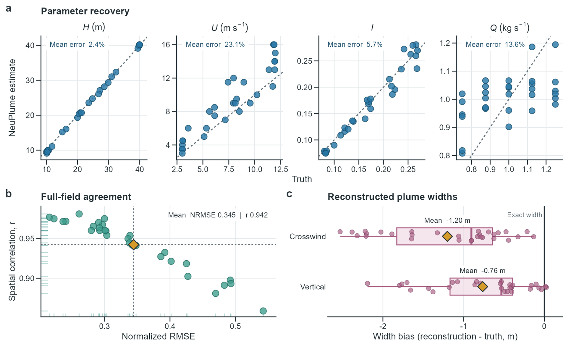
Figure 2 Synthetic validation across 30 held-out cases. (a) Each point is one synthetic case. Estimated values are plotted against the true H, U, I, and Q; dashed diagonal lines denote exact recovery and inset labels give mean absolute relative errors. (b) Joint full-field normalized RMSE and spatial correlation, for which the upper-left direction indicates lower error and stronger spatial agreement; dashed crosshairs and the diamond mark the two sample means. (c) Crosswind and vertical width biases; negative values indicate a narrower reconstruction. Points are cases, boxes show medians and interquartile ranges, and diamonds mark means. Quantitative field metrics use all 100 000 evaluation points.

Figure 3 provides the corresponding three-dimensional comparison for all six preselected representative cases. Across these cases, spatial correlation ranges from 0.918 to 0.981 and centerline displacement ranges from 0.18 to 1.68 m. The complete 30-case summary and the physical conditions of the six cases are reported in Appendix B.

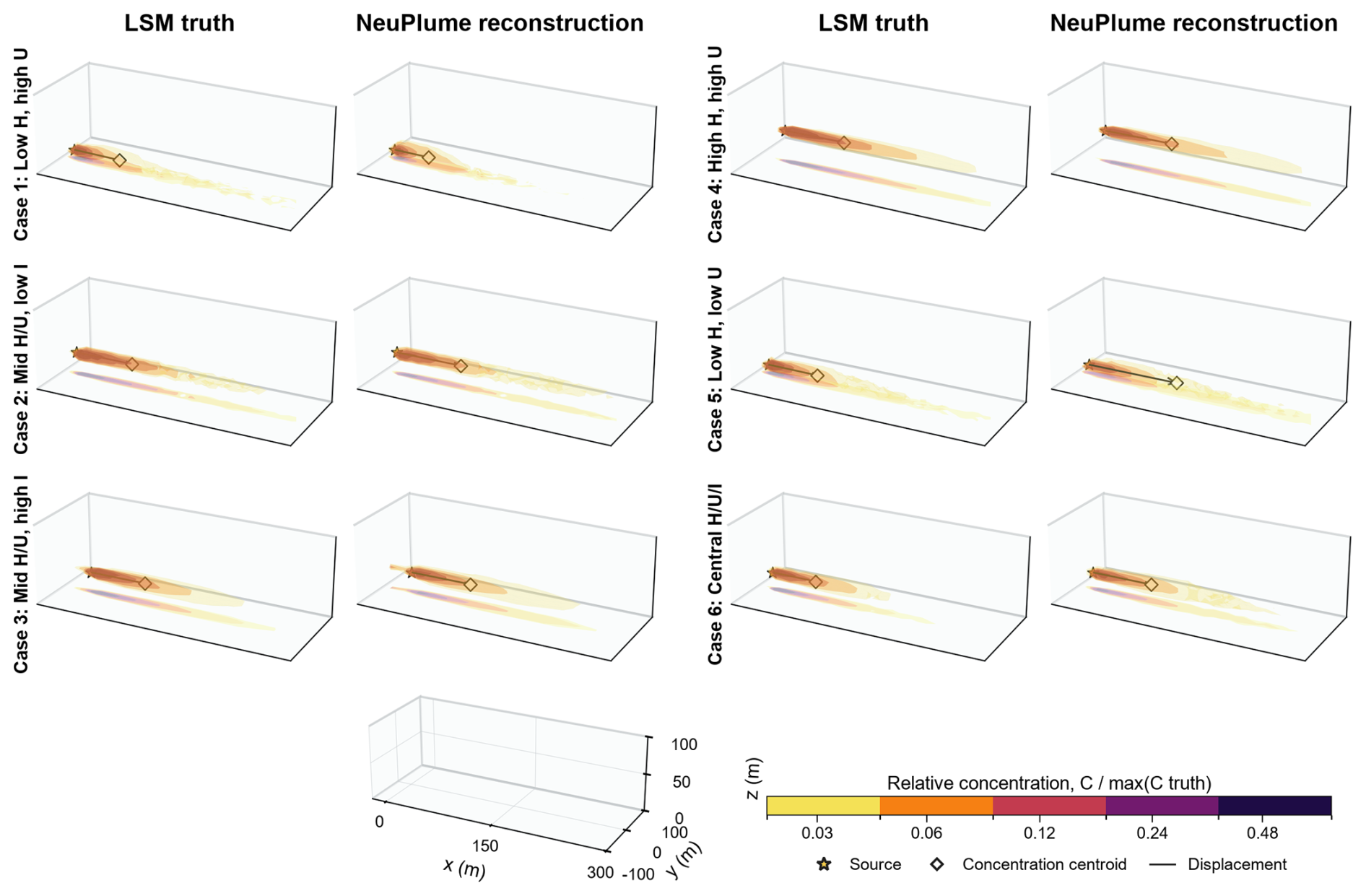
Figure 3 Three-dimensional plume comparisons for the six representative cases. The first two columns compare the LSM truth and NeuPlume reconstruction for Cases 1–3: Case 1 (low H, high U), Case 2 (mid $H/U$, low I), and Case 3 (mid $H/U$, high I). The last two columns show the same comparison for Cases 4–6: Case 4 (high H, high U), Case 5 (low H, low U), and Case 6 (central $H/U/I$). Nested isosurfaces show the three-dimensional concentration field, with maximum-concentration projections on the ground and rear planes. Color and opacity denote $C/max\left(C_{\text{truth}}\right)$ within each case; values below 0.02 are omitted for visibility. Stars mark the source location at the case-specific effective release height, diamonds mark the concentration-weighted centroid of the displayed volume bins, and lines show their displacement. The display uses $\mathrm{52}\times \mathrm{30}\times \mathrm{20}$ bins reconstructed from all 100 000 evaluation points.

4.1.1 Six-case benchmark results

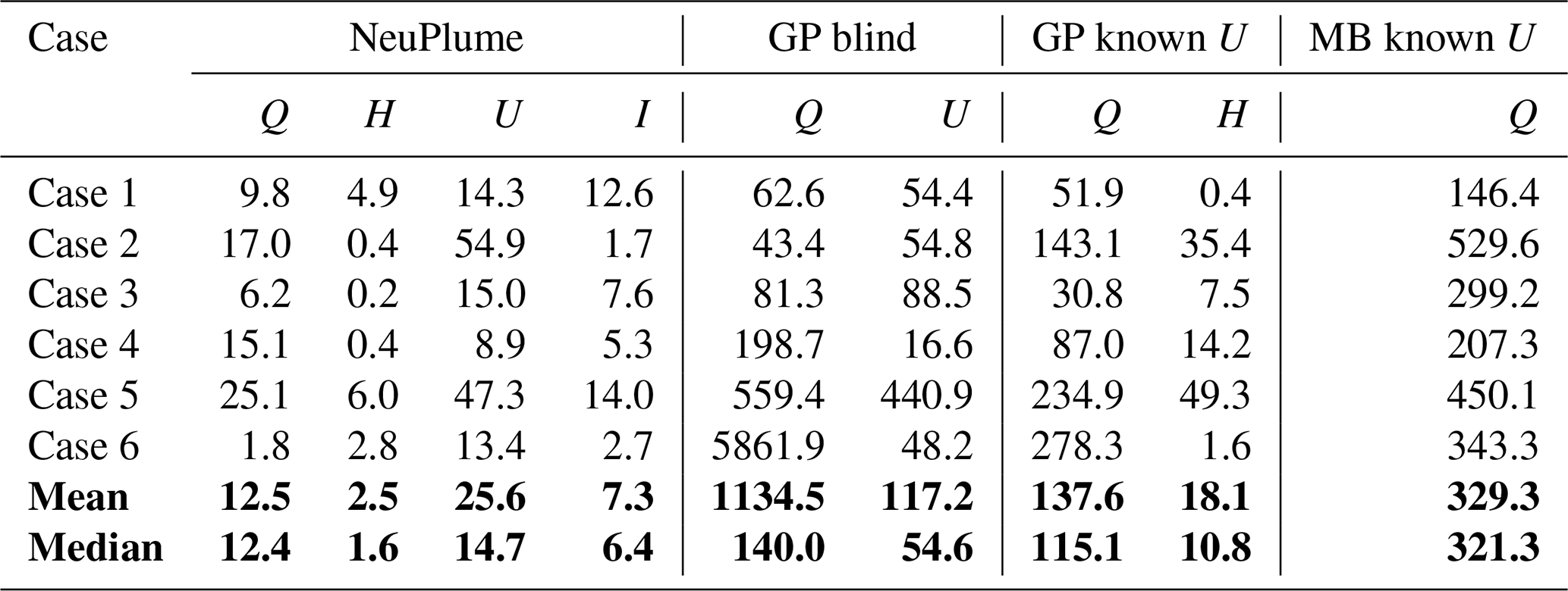
The six representative cases support the GP and MB comparisons, Gaussian-plume control, and coarse-to-fine analysis (Table 1). Across these cases, NeuPlume's mean absolute relative errors are 12.5 % for Q, 2.5 % for H, 25.6 % for U, and 7.3 % for I.

Table 1 Inversion results for the six representative cases. Values are absolute relative errors (%) against true values. NeuPlume, GP, and MB use the same 1000 random-volume observations. Bold rows show the mean and median across the six cases.

The fine stage selects a lower minimum loss in every case. Across the six cases, mean minimum loss decreases from 0.172 to 0.142; the case-wise decrease ranges from 0.001 to 0.080. Figure B1 reports the case-wise changes and the coarse and local fine parameter spaces for the largest- and smallest-improvement cases. Table 1 reports the corresponding parameter accuracy.

4.1.2 Baseline comparison

NeuPlume, GP regression (Shah et al., 2019), and the MB method are applied to the same observations from the six representative cases. Under this random volumetric geometry, mean Q error is 1134.5 % for blind GP, 137.6 % for known-U GP, 329.3 % for known-U MB, and 12.5 % for NeuPlume; the corresponding medians are 140.0 %, 115.1 %, 321.3 %, and 12.4 % (Table 1). The comparison tests how methods designed for analytical plume fitting or cross-sectional flux integration transfer to sparse volumetric observations.

4.1.3 Gaussian plume control experiment

The Gaussian-plume control uses the same source parameters as the six representative cases and generates observations with an analytical Gaussian-plume model (Table C1). In known-U mode, GP recovers all six cases with Q and H errors below 0.001 %. In blind mode, its mean Q and U errors are both 126.3 %, consistent with the Q–U ambiguity when both parameters are inferred from the Gaussian-plume equation. The known-U result confirms that the GP implementation recovers parameters when its field assumption matches the data generator.

4.1.4 Observation geometry and transport-model mismatch

The geometry and transport stress tests use the six representative conditions within the trained parameter support. Figure F1 shows the case-wise transport-mismatch changes, Fig. G1 shows the transformed UAV sampling geometries, and Fig. G2 shows their case-wise degradation relative to random-volume sampling.

With 1000 random-volume observations per case, the mean errors in H, U, I, and Q are 2.46 %, 25.63 %, 7.31 %, and 12.51 %, respectively; mean full-field normalized RMSE is 0.322 and spatial correlation is 0.957. The complete, partial, and off-center trajectory protocols use the same point budget. Their mean normalized RMSE values are 0.744, 0.565, and 0.611, while mean spatial correlations are 0.622, 0.803, and 0.817. Mean I error exceeds 23 % for all three trajectory protocols. The ordering varies by metric: the complete trajectory has the largest mean H error and normalized RMSE, the partial trajectory has the largest mean U and Q errors, and the off-center trajectory has the largest mean I error.

Under strong shear, mean H and U errors increase from 2.46 % and 25.63 % to 3.44 % and 27.41 %, whereas mean I and Q errors decrease slightly to 7.20 % and 9.40 %. Mean full-field normalized RMSE changes from 0.322 to 0.308 and spatial correlation from 0.957 to 0.953. Effective plume rise produces a different response: mean H and U errors increase to 22.72 % and 35.12 %, mean I and Q errors are 8.78 % and 11.83 %, normalized RMSE increases to 0.518, and spatial correlation decreases to 0.821.

4.2 Matched component comparison

We compare full NeuPlume with two references using the same six representative cases, 1000 random-volume observations per case, and loss definition (Fig. 4). The CNF library search removes diffusion and evaluates learned latent fields directly on the same coarse-to-fine parameter grid. Relative to this reference, full NeuPlume reduces the mean errors in H, U, I, and Q from 3.21 %, 49.36 %, 22.10 %, and 18.54 % to 2.46 %, 25.63 %, 7.31 %, and 12.51 %, respectively. Mean normalized RMSE decreases from 0.438 to 0.322, and spatial correlation increases from 0.910 to 0.957. These matched results show that diffusion improves parameter selection and full-field reconstruction relative to direct CNF library search under the tested protocol.

Direct LSM search evaluates the 1 000-member physical library against the off-grid representative truth fields and provides a finite-library lookup reference. It attains a mean normalized RMSE of 0.178 and a mean spatial correlation of 0.981. Its remaining parameter errors (H: 1.62 %, U: 17.79 %, I: 11.41 %, Q: 22.91 %) quantify discretization and parameter ambiguity in this same-simulator lookup.

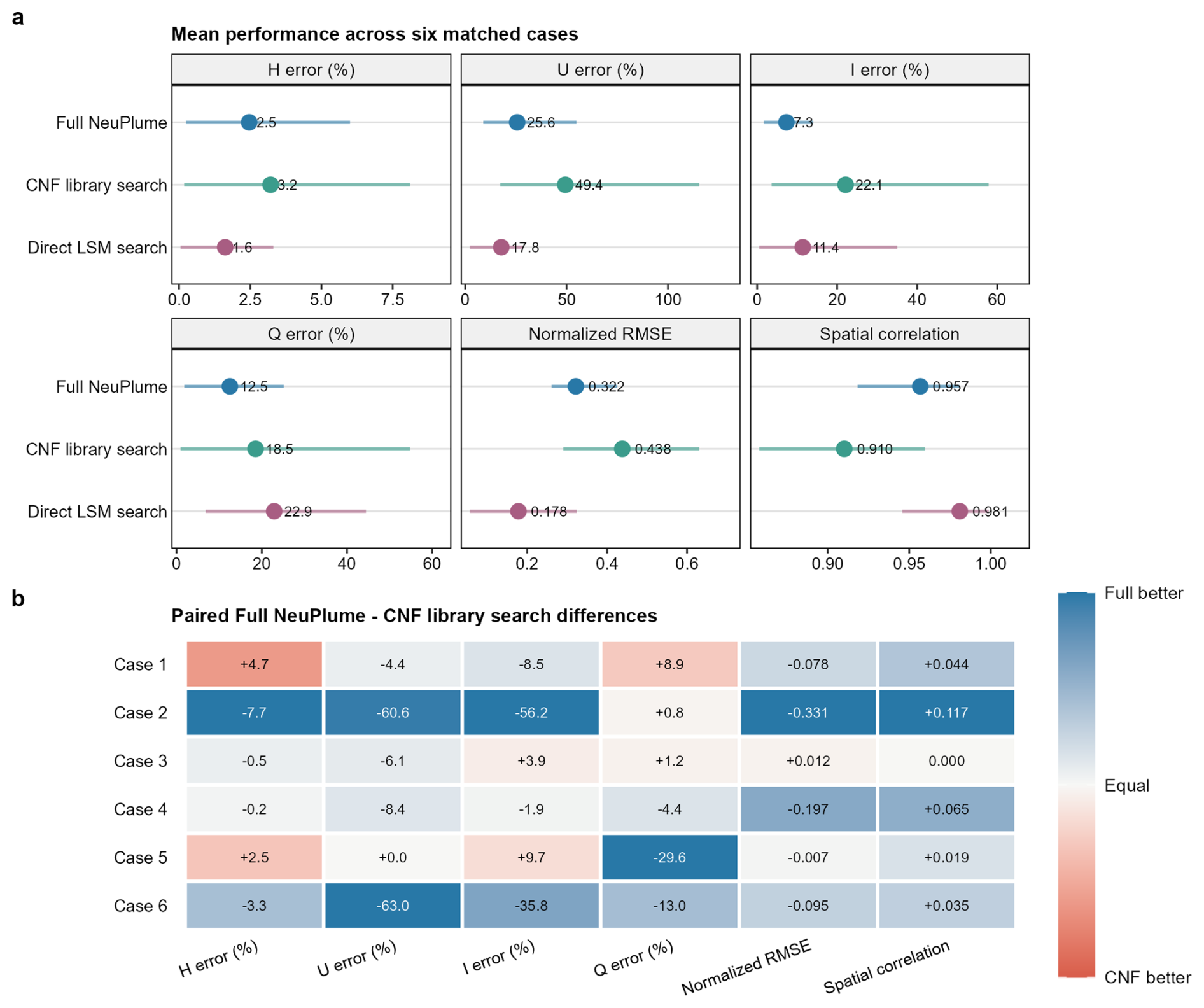
Figure 4 Matched accuracy comparison for the six representative cases. (a) Mean absolute relative errors for effective release height H, wind speed U, turbulence intensity I, and emission rate Q, together with mean full-field normalized RMSE and spatial correlation; horizontal intervals span the minimum to maximum across the six cases. (b) Case-wise paired differences between Full NeuPlume and CNF library search. Cell labels report the raw Full NeuPlume minus CNF library search difference in the units of each metric. Colour direction is oriented so that blue denotes better Full NeuPlume performance and orange denotes better CNF library-search performance, with intensity scaled separately within each metric. Lower values indicate better performance for the four parameter errors and normalized RMSE; higher values indicate better spatial correlation. Direct LSM search is a finite-library lookup reference whose 1000 candidates do not contain the six truth conditions.

4.3 Real-data case study

We evaluate the Pniówek V flights in known-U and blind modes. The same-shaft hourly inventory ($\mathrm{13.3}\pm \mathrm{4.1}\mathrm{kt}{\mathrm{yr}}^{-\mathrm{1}}$) provides the primary descriptive reference. Campaign-level IG ($\mathrm{9.5}\pm \mathrm{3.5}\mathrm{kt}{\mathrm{yr}}^{-\mathrm{1}}$) and MB ($\mathrm{9.8}\pm \mathrm{5.0}\mathrm{kt}{\mathrm{yr}}^{-\mathrm{1}}$) estimates provide additional references (Andersen et al., 2023). Table 2 and Fig. 5 report NeuPlume's selected minimum-loss estimates.

Table 2 Minimum-loss NeuPlume estimates for the Pniówek V flights. Known-U fixes wind speed to the meteorological-station value; blind inversion selects Q and U jointly.

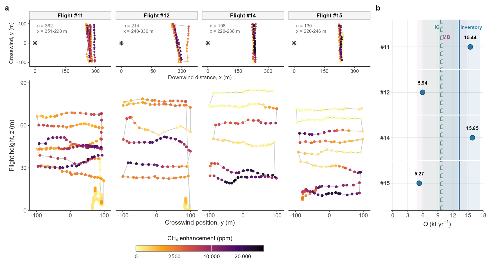
Figure 5 Real-data inversion for the Pniówek V ventilation shaft. (a) UAV sampling geometry for each flight. The upper strips locate the observations in the downwind–crosswind plane; stars mark the shaft. The lower panels show the crosswind–height sampling curtains, with grey lines tracing the flight paths and color denoting methane enhancement. Labels report the number of observations and sampled downwind range. (b) NeuPlume known-U minimum-loss Q estimates (points). The same-shaft inventory and published IG and MB values retain their reported external ranges.

Known-U estimates for flights #11 and #14 are 2.14 and 2.55 kt yr⁻¹ above the inventory center and fall within its reported 9.2–17.4 kt yr⁻¹ range. Flights #12 and #15 are 7.36 and 8.03 kt yr⁻¹ below the center and lie 3.26 and 3.93 kt yr⁻¹ below the lower end of that range.

Blind inversion selects lower wind speeds for flights #11, #12, and #14 and correspondingly lower Q values. Flight #15 selects $U=\mathrm{14.0}\mathrm{m}{\mathrm{s}}^{-\mathrm{1}}$, more than twice the station value, and $Q=\mathrm{13.26}\mathrm{kt}{\mathrm{yr}}^{-\mathrm{1}}$. Across all four flights, the selected U and Q move in the same direction relative to the known-U solution.

Known-U inversion selects effective heights of 52.2, 43.8, 3.3, and 9.2 m for flights #11, #12, #14, and #15, respectively. The corresponding blind-mode heights are 61.4, 47.9, 2.2, and 10.6 m.

The GP and our flight-level MB baseline produce substantially larger or smaller point estimates under these sparse trajectories (Table D1). GP blind estimates span 25–1792 kt yr⁻¹ and GP known-U estimates span 31–49 kt yr⁻¹, while MB estimates span 0.009–0.055 kt yr⁻¹. NeuPlume known-U estimates span 5.27–15.85 kt yr⁻¹.

5 Discussion

The 30-case validation shows that NeuPlume preserves plume location and large-scale spatial organization more reliably than cross-sectional spread. Strong positional agreement together with negative mean width bias identifies cross-sectional spread as the systematic field-reconstruction error. In the six representative cases, NeuPlume also yields lower mean emission-rate error than GP and MB under random volumetric sampling. This comparison establishes NeuPlume's advantage for emission-rate estimation under the tested sparse three-dimensional observation geometry.

5.1 Measurement geometry, wind representativeness, and identifiability

The field inversions expose strong coupling between wind-speed representativeness and the selected emission rate. Because the CNF represents unit-emission fields, the fitted source strength scales with effective transport speed. Across all four flights, the blind solutions move U and Q in the same direction relative to the known-U solutions. This behavior is consistent with wind sensitivities reported in cross-sectional-flux and controlled-release studies (Meier et al., 2026; Eastwood et al., 2025; Conrad et al., 2023; He et al., 2024).

The controlled geometry test shows that point count alone does not determine performance. Concentrating the matched point budget near transformed UAV trajectories degrades parameter and full-field recovery on average relative to random-volume sampling (Figs. G1 and G2). Each trajectory protocol represents a compound sampling pattern, but their common contrast with the matched random-volume protocol supports a clear measurement objective: sample multiple downwind positions, obtain crosswind and vertical contrast, and record wind over the plume-transport scale. UAV studies likewise identify plume coverage, platform configuration, and wind sampling as major determinants of emission accuracy (Liu et al., 2024; Mohammadloo et al., 2025; Vollrath et al., 2026; Scheutz et al., 2025).

5.2 Physical scope and boundary effects

The present implementation and validation cover passive, low-height, neutral releases over flat terrain. The current forward model uses open boundaries. Within this parameterization, H is an effective release height that can absorb unrepresented vertical transport. Flights #11 and #12 select heights near or above the 50 m training-grid ceiling after continuous refinement, marking the edge of the trained height support. The present observations do not resolve which omitted transport process produces these boundary solutions.

The two transport stress tests show why field agreement and parameter identification must be assessed separately. Strong shear changes the selected simple-model parameters without a corresponding mean loss of full-field similarity, whereas effective plume rise degrades both parameter and field recovery. In the plume-rise test, H absorbs part of the missing vertical transport and functions as an effective height rather than a physical outlet elevation.

Open-boundary diagnostics in Table E1 show that most particle exits occur through the downwind boundary and quantify the smaller side and top losses. Measurements and forward domains for weak-wind or high-turbulence regimes require sufficient crosswind and vertical extent to capture the broader plume. The current LSM also excludes flow regimes in which material exits and later re-enters through recirculation or building wakes.

The forward-library design defines a direct extension path for additional regimes. Stable and unstable boundary layers require stability-conditioned simulations because they alter wind shear, vertical exchange, turbulent-velocity distributions, and the LSM drift needed to satisfy the well-mixed condition (Newman and Klein, 2014; Cassiani et al., 2014). Time-varying releases require a temporally resolved library and field representation, for which sequential Bayesian source-term methods provide an established reference (Xu et al., 2025).

5.3 Method positioning and validation

NeuPlume targets near-field settings where a simulation-trained representation can describe non-Gaussian structure and several source and environmental parameters must be searched jointly. GP and MB remain efficient choices when their plume and sampling assumptions hold (Shah et al., 2019; Krings et al., 2013; Conley et al., 2017). The field comparison here is therefore descriptive: without a flight-specific certified emission rate, the spread among NeuPlume, GP, and MB estimates cannot establish absolute accuracy. A controlled-release experiment with a known reference emission rate for each flight would provide the decisive test of NeuPlume's absolute emission-rate accuracy under field conditions (Morales et al., 2022; Vollrath et al., 2026). Such validation should span wind regimes and observation geometries while retaining the minimum-loss selection rule used here.

6 Conclusions

NeuPlume estimates point-source parameters and complete three-dimensional concentration fields from sparse observations by searching a generative representation of LSM simulations. Across 30 held-out synthetic cases, fields retained plume-scale spatial organization (mean spatial correlation, 0.942), and emission-rate error averaged 13.6 %; reconstructed plumes remained systematically narrow. In six matched cases, diffusion improved parameter and field metrics over direct CNF library search, and NeuPlume reduced emission-rate error relative to GP and MB under random-volume sampling.

Stress tests identified observation geometry and forward-model fidelity as distinct controls. UAV-like trajectories weakened field reconstruction at the same observation budget. Under transport mismatch, shear shifted parameters while preserving mean field similarity, whereas effective plume rise degraded parameter and field recovery. The Pniówek inversions exposed a positive wind-speed–emission-rate coupling: higher selected wind speeds required larger emission-rate estimates to reproduce the observed concentration enhancements, whereas lower selected wind speeds produced lower estimates. NeuPlume thus provides an extensible framework for jointly estimating source parameters and concentration fields. The framework was validated here for passive, low-height, neutral releases over flat terrain; additional transport regimes can be incorporated through regime-specific simulation ensembles and neural-model retraining.

Appendix A: Training and inversion hyperparameters

Table A1 lists the neural representation, diffusion training, candidate-generation, coarse-to-fine search, and emission-rate refinement settings used in the reported experiments. The real-data experiments use the same DPS settings, search I_ref on a discrete grid, and set n_fine=3.

Table A1 Training and inversion hyperparameters of the NeuPlume framework.

Appendix B: Detailed synthetic validation

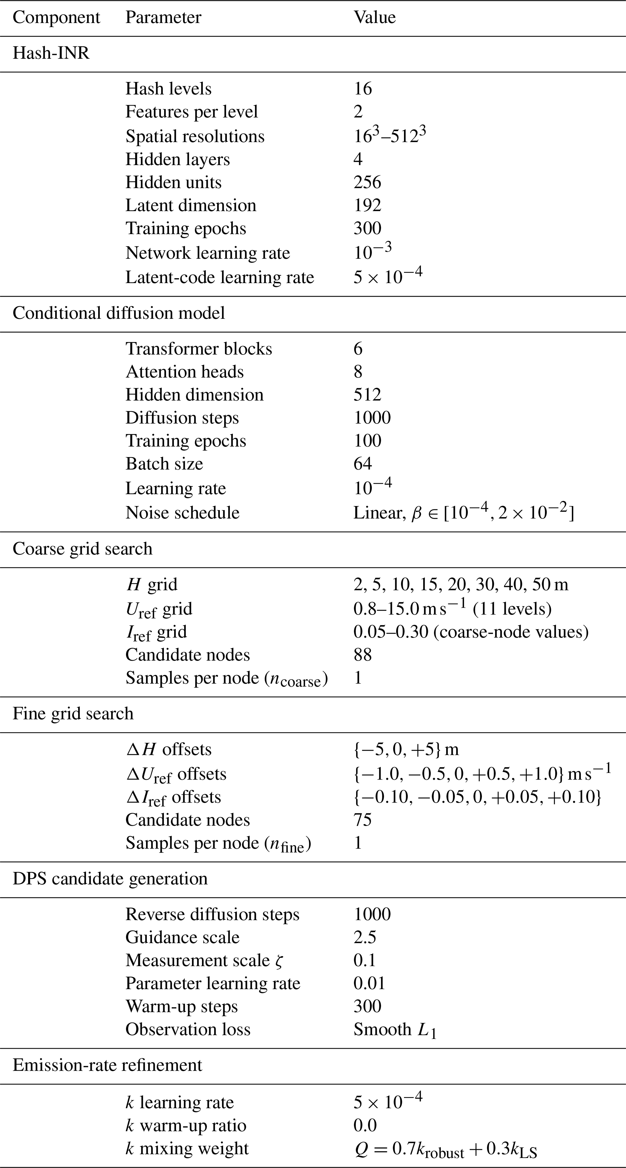
Table B1 gives the complete 30-case parameter and field summary. Table B2 lists the physical conditions of the six preselected representative cases used for method comparisons and controlled stress tests. Figure B1 reports the coarse-to-fine observation-mismatch results.

Table B1 Performance across the 30-case synthetic validation set. Parameter rows report absolute relative error. Field rows compare the selected concentration field with the LSM truth. Width bias is reconstruction minus truth, so negative values indicate a narrower reconstructed plume. n/a: not applicable.

Table B2 Physical conditions for the six representative cases.

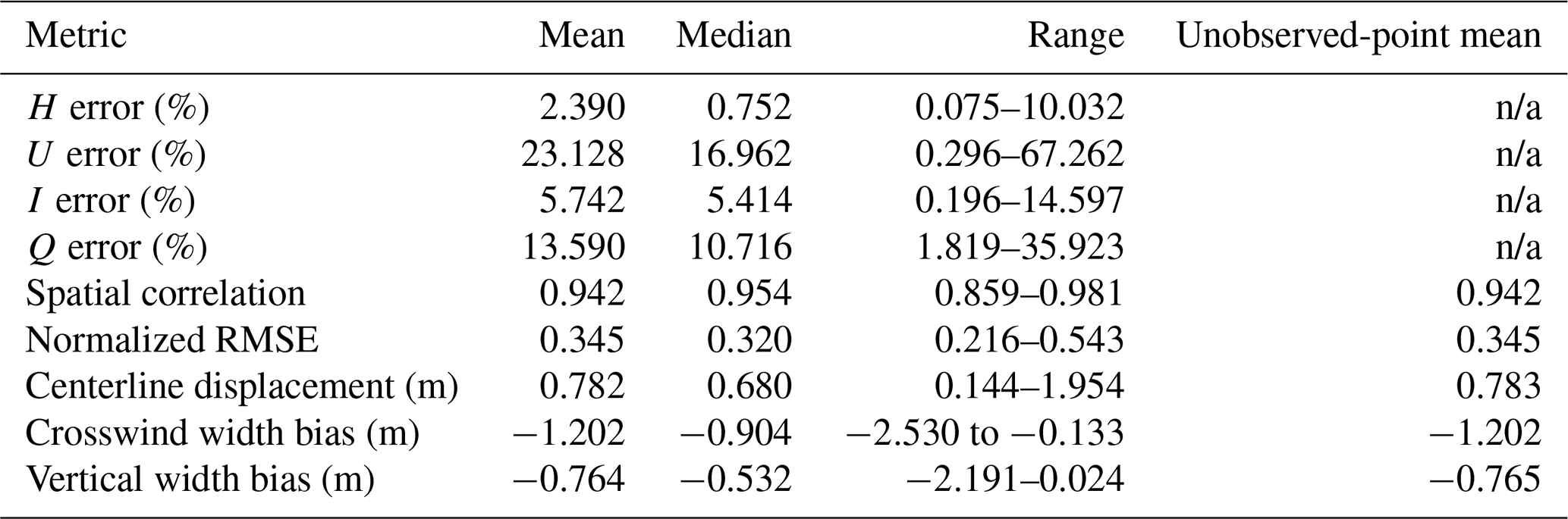
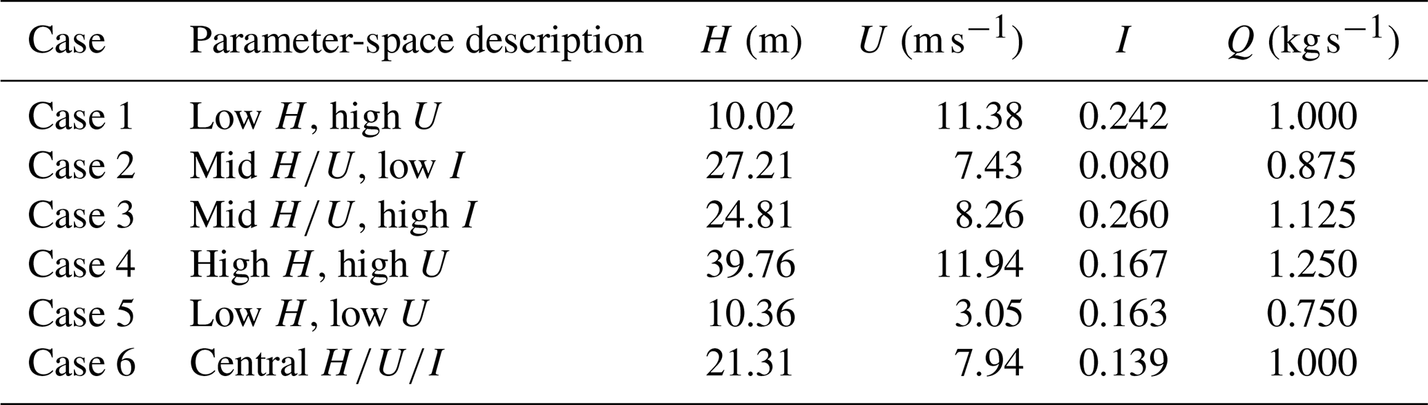
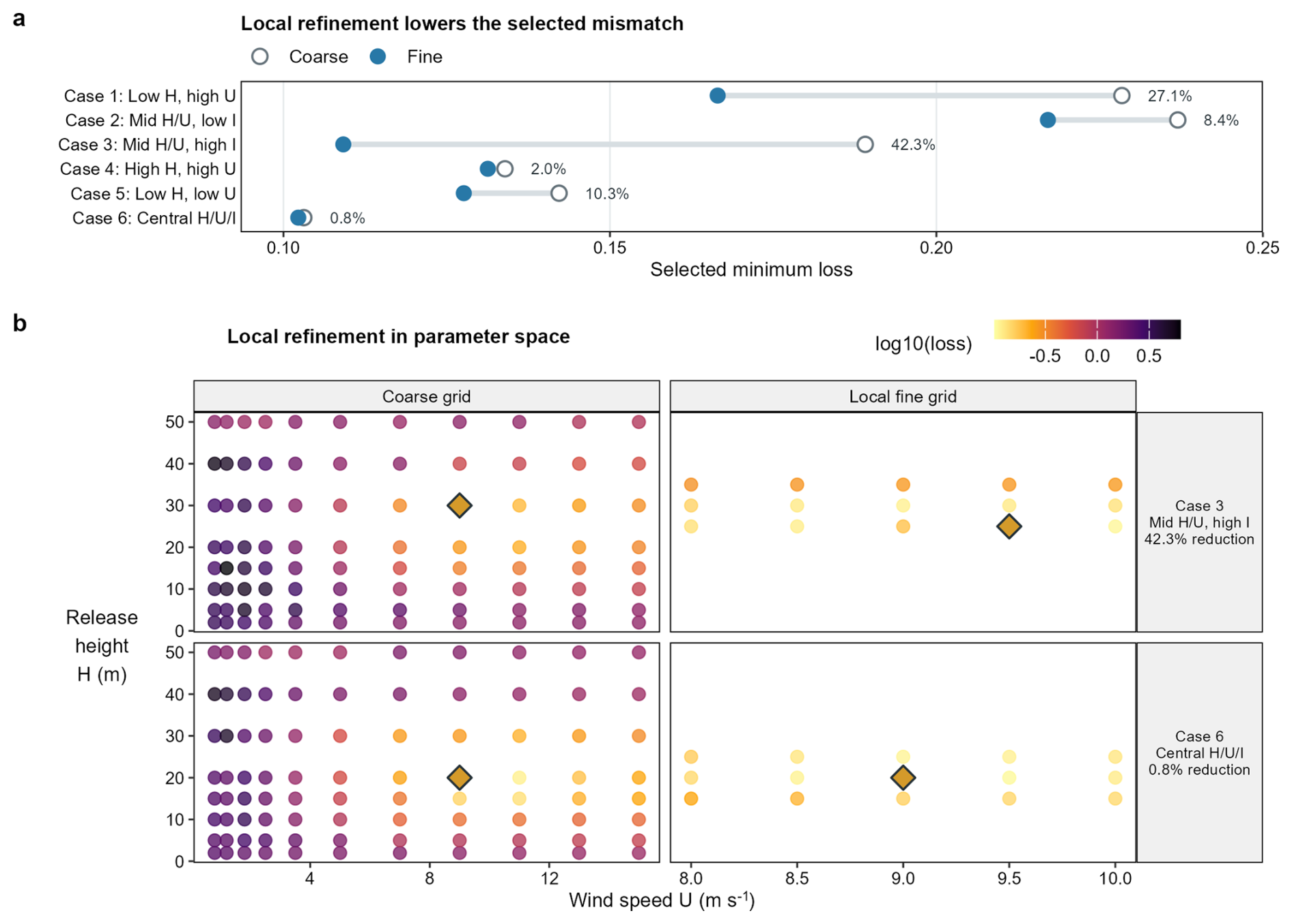
Figure B1 Coarse-to-fine optimization of the observation-mismatch objective. (a) Selected minimum losses for all six representative cases, ordered by relative reduction. The fine search lowers the selected loss in every case, with reductions from 0.8 % to 42.3 %. Descriptive labels summarize each case's location in the H–U–I parameter domain. (b) Coarse and local fine H–U search spaces for Case 3 (mid $H/U$, high I) and Case 6 (central $H/U/I$), which have the largest and smallest reductions, respectively. Coarse points show node losses; fine-grid color shows the minimum loss across candidate I values at each H–U location. Yellow diamonds mark the selected node at each stage. Each case has 88 coarse and 75 fine nodes.

Appendix C: Gaussian-plume control

Table C1 reports the Gaussian-plume control for the six representative source conditions. The analytical Gaussian-plume model generated the observations used in this control.

Table C1 Gaussian-plume control on analytical GP synthetic data. Values are absolute relative errors. Known-U errors below 0.001 % show parameter recovery when the plume model and wind input match the data generator. The bold row shows the mean across the six cases.

Appendix D: Field-data baseline estimates

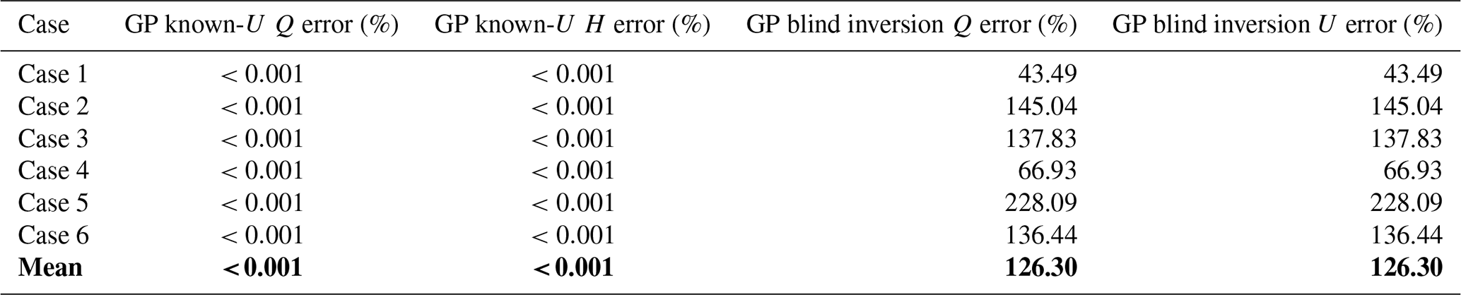
Table D1 reports the flight-level GP and our flight-level MB baseline estimates used to bound the field-data comparison in Sect. 4.3. These values are separate from the published campaign-level MB reference reported in the main text and Fig. 5.

Table D1 GP and MB estimates for the four Pniówek V flights. The same-campaign published IG estimate is $\mathrm{9.5}\pm \mathrm{3.5}\mathrm{kt}{\mathrm{yr}}^{-\mathrm{1}}$.

Appendix E: Boundary-loss diagnostics

The LSM open-boundary accounting provides the physical-domain diagnostic discussed in Sect. 5.2.

Table E1 Boundary-loss diagnostics for the six representative cases using the LSM configuration specified in Sect. 2.2 and a unit emission rate.

Appendix F: Transport-model mismatch

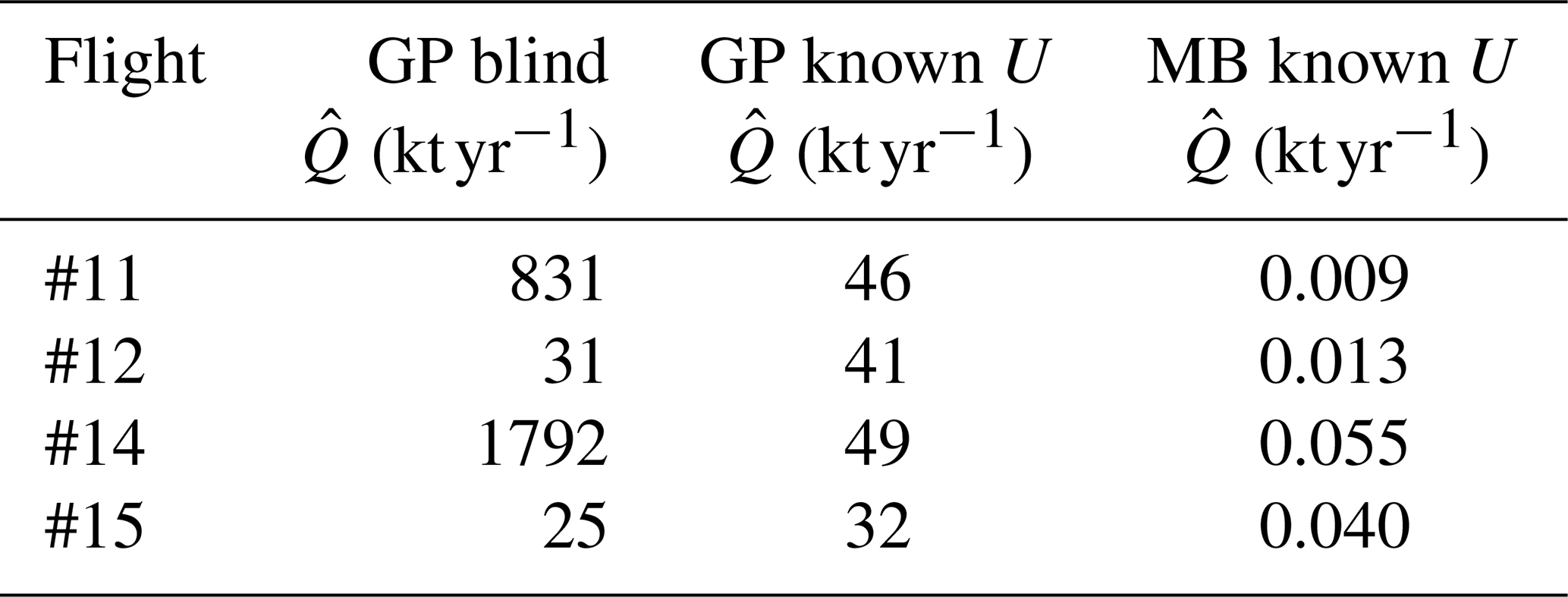
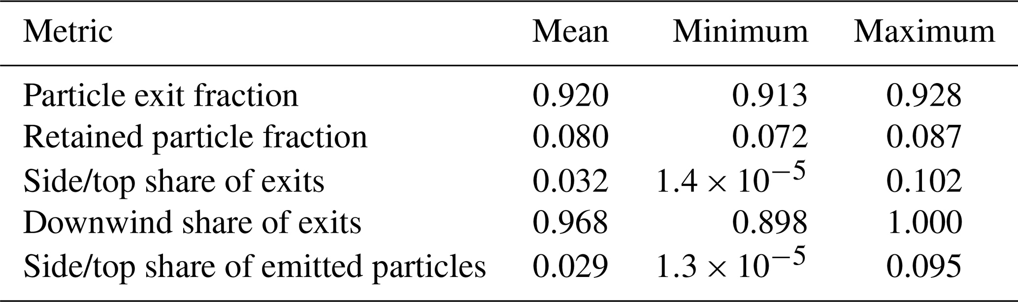
Figure F1 reports the case-wise changes produced by strong shear and effective plume rise relative to the matched simple-transport baseline.

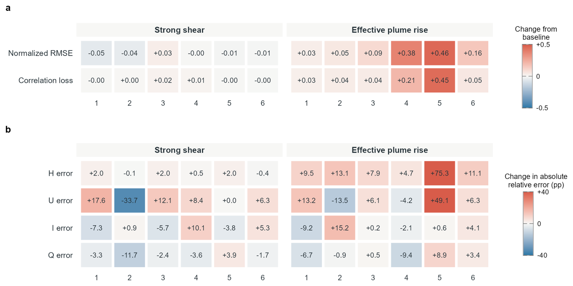
Figure F1 Controlled transport-mismatch stress tests across six representative conditions within the trained parameter support. Rows show changes in normalized RMSE, correlation loss, and the absolute relative errors of H, U, I, and Q; columns identify Cases 1–6 for each mismatch condition. Changes are relative to each case's simple-transport baseline under the same 1 % random-volume observation mask. Positive values denote worse performance, with correlation loss defined as baseline minus tested spatial correlation. Cell labels report untruncated changes; parameter-error colors are truncated at ±40 percentage points to preserve contrast.

Appendix G: Observation-geometry stress test

Figure G1 defines the three transformed UAV sampling protocols, and Fig. G2 reports their case-wise changes relative to matched random-volume sampling.

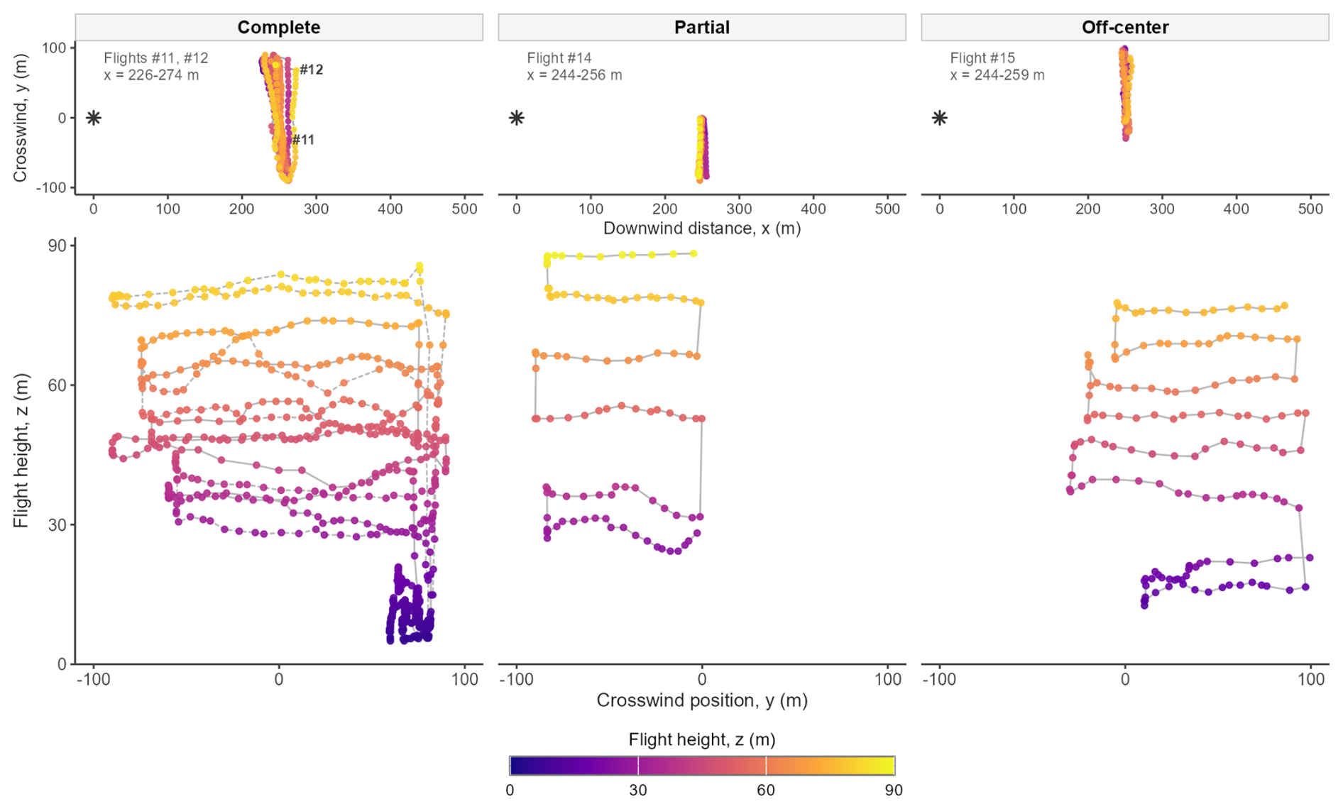
Figure G1 Complete, partial, and off-center transformed UAV sampling trajectories used in the controlled observation-geometry stress test. The upper strips locate the trajectories in the downwind–crosswind plane; stars mark the source and annotations identify the source flights and sampled downwind ranges. The lower panels show the crosswind–height sampling curtains. Color denotes flight height. Each protocol uses a different source flight and transformation and therefore represents a compound sampling geometry.

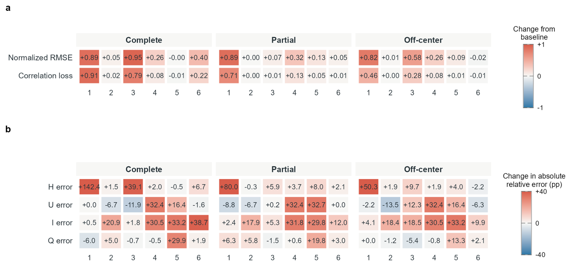
Figure G2 Case-wise degradation under three transformed UAV sampling protocols across six representative conditions. Rows show changes in normalized RMSE, correlation loss, and the absolute relative errors of H, U, I, and Q; columns identify Cases 1–6 for each protocol. Changes are relative to each case's matched 1,000-point random-volume baseline. Positive values denote worse performance, with correlation loss defined as baseline minus tested spatial correlation. Cell labels report untruncated changes; parameter-error colors are truncated at ±40 percentage points to preserve contrast. Each protocol combines a different source flight and transformation and therefore represents a compound geometry.