Fire carbon emission constraints from space-based carbon monoxide retrievals during the 2019 intense burning season in Brazil

In 2019, Brazil experienced an intensive fire season, despite the absence of major climate anomalies to enhance fire activity. Existing carbon monoxide (CO) emission estimates from state-of-the-art fire emission inventories differ by a factor two for the period and region. We provide a top-down estimate on CO emissions from these fires using the new CarbonTracker Europe – Long-Window/Short-Window (CTE-LW/SW) inverse modelling framework driven by column-averaged dry air CO mole fractions (X_CO) from the MOPITT and TROPOMI satellite instruments.

Our analysis indicates that the 2019 fires in Brazil released approximately 47 TgCO. Although structural atmospheric-chemistry related uncertainties remain (±15 TgCO), the inversions converged strongly to a common posterior (46–48 TgCO) independent of the prior emission inventory (GFED5.1, GFAS v1.2) or assimilated dataset (TROPOMI, MOPITT).

Posterior fire emissions closely resemble the newly released GFED5.1, supporting recent advances in bottom-up fire modelling. Nonetheless, at the biome level, our results reveal a systematic underestimation – by roughly a factor of two – in the Cerrado and Caatinga savannas relative to both fire emission priors. While more targeted uncertainty assessments are required, we speculate that this emission gap unlikely stems from inversion choices alone and may indicate an underestimation of fuel loads or emission factors.

Overall, we demonstrate CTE-LW/SW effectively leverages X_CO to complement existing fire emission monitoring capacities at increasingly fine spatial resolution – a capability that is especially valuable in Brazil, where different fire regimes occur in close proximity and fire activity has intensified in recent years.

1 Introduction

In recent years, the Amazon region was subject to intense recurrent fires. These fires have far-reaching consequences for air quality, human health, biodiversity, and the regional carbon balance (e.g. Barlow et al., 2016; Nawaz and Henze, 2020; Friedlingstein et al., 2025). Fire disturbances further pressure the Amazon region to act as net sink, a capacity that growing evidence indicates is weakening (Gatti et al., 2021, 2023; Gloor et al., 2012; Brienen et al., 2015; Phillips et al., 2017; Hubau et al., 2020).

Unlike the adjacent fire-adapted and fire-dependent Cerrado savannas, Amazonian rainforests are not naturally shaped by fire (e.g. Cochrane, 2003; Pivello, 2011). Ignitions predominantly stem from human-driven land-use activities – primarily land clearing through slash-and-burn practices during which forest biomass is felled, dried, and then ignited (e.g. Uhl and Buschbacher, 1985; Morton et al., 2006, 2008). These intentional burns usually produce long-lasting, smouldering fires. Frequently, these escape into adjacent forests and persist as understory fires (e.g. Alencar et al., 2004, 2006; Morton et al., 2013), which contribute to forest degradation (Lapola et al., 2023). Both the deforestation fires themselves and the degradation that follows release large amounts of carbon into the atmosphere, impacting carbon cycling on immediate to multi-decadal timescales (e.g. van der Werf et al., 2017; Lapola et al., 2023; Qin et al., 2021; Bourgoin et al., 2024).

On top of anthropogenic pressures, environmental conditions, such as droughts, increase the susceptibility of the fire-sensitive Amazonian forests to burning (e.g. Brando et al., 2014). Dry seasons in Amazonia are becoming longer and more intense (Marengo et al., 2018; Wainwright et al., 2022). The forests increasingly experience drought–heatwave events that are more frequent, longer lasting, more extensive, and compounded by low soil moisture/high vapour-pressure deficit conditions (Ferreira et al., 2025). Climate projections from CMIP6 models indicate continued declines in rainfall, particularly in the southeastern Amazon, alongside hotter and longer droughts (Parsons, 2020; Ukkola et al., 2020). Fire-conducive weather conditions are becoming more frequent and extreme (Jolly et al., 2015; Jones et al., 2022), and projections indicate further increases – especially for extreme events (Jones et al., 2022). Even if the rate of deforestation declines, reductions in fire frequency (Le Page et al., 2017) and related carbon emissions (Aragão et al., 2018) are unlikely.

After more than a decade of declining deforestation rates, and in the absence of abnormal drought conditions, Amazonian fire activity rose sharply again in 2019. The fires drew the attention of the global media and scientists due to their scale and visibility (e.g. Silveira et al., 2020; Lizundia-Loiola et al., 2020; Brando et al., 2020a; Cardil et al., 2020; Kelley et al., 2021; Andela et al., 2022; Barlow et al., 2020; Escobar, 2019; Arruda et al., 2019), and rekindled concerns about increasing risks of large-scale forest dieback (Lovejoy and Nobre, 2019; Brando et al., 2020b). Fire emission estimates for this period were made, among others, by bottom-up fire emission models like the Global Fire Emissions Database (GFED, van der Werf et al., 2017, 2025) and Global Fire Assimilation System (GFAS, Kaiser et al., 2012), relying on burned area data coupled with a vegetation model or fire radiative power (FRP) data, respectively.

These fire emission models have advanced our understanding of fire dynamics and the emissions they produce. While significant progress has been made, important questions remain regarding their accuracy to estimate emission magnitudes, especially under challenging observational conditions (e.g. persistent cloud cover, below-canopy fires). A proper uncertainty quantification therefore remains challenging. Through its co-release with carbon dioxide (CO₂) during incomplete combustion, carbon monoxide (CO) serves as tracer of fire activity. Fire-induced CO enhancements stand out against a relatively low background, making atmospheric CO observations a valuable proxy for total carbon emissions. Atmospheric modelling of CO provides an independent means to evaluate bottom-up fire inventories. When taken a step further through satellite driven inverse modelling, it can offer a powerful, complementary constraint on fire emissions.

Early atmospheric CO inversion studies relied on sparse surface measurements, which rarely captured fire plumes and thus placed little emphasis on optimizing fire emissions (Bergamaschi et al., 2000; Kasibhatla et al., 2002; Pétron et al., 2002; Pison et al., 2009; Hooghiemstra et al., 2011; Palmer et al., 2003), with the exception of a surface-based CO inversion by van der Werf et al. (2004), which despite its simplicity, proved effective in informing on continental scale fire emission anomalies and aided to improve the first global fire emissions data base (GFED) inventory estimates. The arrival of space-based CO retrievals – most notably from the Measurements of Pollution In The Troposphere (MOPITT), Tropospheric Emission Spectrometer (TES), and Infrared Atmospheric Sounding Interferometer (IASI) instruments – facilitated more systematic observations of fire plumes and brought fire emissions more to the forefront of inversion analyses. They especially helped to better understand the timing and magnitude of fire emissions (Heald et al., 2004; Pétron et al., 2004; Pfister et al., 2005; Arellano et al., 2006; Chevallier et al., 2009; Jones et al., 2009; Gonzi et al., 2011; Krol et al., 2013; Bloom et al., 2015; Yin et al., 2016; Nechita-Banda et al., 2018; Jiang et al., 2017; Zheng et al., 2018; Naus et al., 2022; Peiro et al., 2022; Zheng et al., 2023).

Advances in satellite retrieval algorithms and the introduction of new instruments such as the TROPOspheric Monitoring Instrument aboard ESA’s Copernicus Sentinel-5 Precursor satellite (S5P-TROPOMI), constantly improve our capability to infer atmospheric CO abundances from space. These developments provide new opportunities to investigate fire emissions and their dynamics at increasingly higher spatial and temporal resolutions, as already demonstrated by for example van der Velde et al. (2021b, a), Byrne et al. (2021, 2024), Goudar et al. (2023), Nüß et al. (2025), Griffin et al. (2024), Forkel et al. (2025), Voshtani et al. (2025), Nguyen et al. (2023).

Despite these advances, few atmospheric CO inversion studies have focused specifically on South American fires (van der Laan‐Luijkx et al., 2015; Bowman et al., 2017; Hooghiemstra et al., 2012b; Naus et al., 2022), and none have studied the added value of TROPOMI observations for this region using a formal inversion. In this study, we provide fire CO emission estimates for the 2019 fires in Brazil using constraints from satellite column average CO mole fraction (X_CO) data using a novel inversion system. Our objectives are to (i) quantify the spatial and temporal distribution of CO fire emissions across different biome types, (ii) assess the consistency of TROPOMI constraints w.r.t. MOPITT, and (iii) evaluate fire emission modelling efforts for Brazilian fires with the inversion results. This work contributes to improve our understanding of the carbon impact of (extreme) fire events in the Amazon region to support future mitigation and monitoring strategies.

In the following sections, we first describe the new data assimilation framework and datasets used (Sect. 2). Subsequently, we demonstrate the performance of our system for the 2019 fire season, as an example of an intense fire year, by comparing our results with independent datasets (Sect. 3.1). We present the spatial and temporal overview of 2019 fire emissions (Sect. 3.2–3.3). We conclude with a discussion of our results and their implications for future fire emission quantification.

2 Methods and data description

2.1 The CTE-LW/SW inversion system for CO

To optimise South American fire emissions using satellite retrievals, we apply a two-step inversion framework consisting of a long-window (LW) and a short-window (SW) inversion. The LW inversion resolves monthly to inter-annual variability in the global CO budget, while the SW inversion targets daily variability in fire emissions. Decoupling the system in this way allows each step to use a set of observations that target spatio-temporal scales for source/sink processes of interest through the design of a statevector. We implement this approach in the CarbonTracker Data Assimilation Shell (CTDAS; van der Laan-Luijkx et al., 2017), building on the CarbonTracker Europe (CTE) ensemble Kalman smoother around the TM5 transport model (Peters et al., 2005).

The long-window inversion approach was recently developed for CO₂ and related tracers (van der Woude, 2024). Here, we present the first application that expands this LW system to CO. Subsequently, we designed and performed a short-window inversion for CO and refer to the combined system as CTE-LW/SW. We model atmospheric CO using the following the mass balance equation:

$$\begin{array}{}\text{(1)}& \begin{array}{rl}& {\displaystyle \frac{{\mathrm{dCO}}_{(x,y,z,t)}}{\mathrm{d}t}}=\stackrel{\text{short-window}}{\overbrace{{\mathit{\lambda }}_{r,t}^{\mathrm{fire}}}}\cdot E_{(x,y,t)}^{\mathrm{fire}}\\ & +\stackrel{\text{long-window}}{\overbrace{\overbrace{{\mathit{\lambda }}_{r,t}^{\mathrm{NMVOC}}}\cdot P_{(x,y,z,t)}^{\mathrm{NMVOC}}+\overbrace{{\mathit{\lambda }}_{r,t}^{{\mathrm{CH}}_{\mathrm{4}}}}\cdot P_{(x,y,z,t)}^{{\mathrm{CH}}_{\mathrm{4}}}+\overbrace{{\mathit{\lambda }}_{r,t}^{\mathrm{ant}}}}}\cdot E_{(x,y,t)}^{\mathrm{ant}}\\ & -L_{(x,y,z,t)}^{\mathrm{CO}+\mathrm{OH}}-D_{(x,y,t)}^{\mathrm{dry}}\end{array}\end{array}$$

where E^fire, E^ant represent emissions from fires and anthropogenic activities. P^NMVOC, and $P^{{\mathrm{CH}}_{\mathrm{4}}}$ stand for the chemical CO production through the oxidation of methane (CH₄) and non-methane volatile organic compounds (NMVOCs). Chemical loss of CO by the hydroxyl radical (OH; L^CO+OH) and dry deposition (D^dry) are calculated online in the atmospheric transport model that acts as observation operator (details in Sect. 2.3). The λ's represent a set of linear scaling factors for each source term for a given set of statevector elements (r) that are optimised in the indicated assimilation step (Table 1).

First, we optimise ${\mathit{\lambda }}_{r,t}^{\mathrm{NMVOC}}$, ${\mathit{\lambda }}_{r,t}^{{\mathrm{CH}}_{\mathrm{4}}}$, and ${\mathit{\lambda }}_{r,t}^{\mathrm{ant}}$ in the global-scale long-window inversion using flask observations from the National Oceanic and Atmospheric Administration Global Monitoring Laboratory (NOAA-GML) GLOBALVIEWplus v4.0 ObsPack (Schuldt et al., 2024). This step focuses on the capturing the monthly to inter-annual variation in the CO budget components (excluding fire emissions) using the background flask network. The long-window inversion then provides a set of optimised fluxes that serve as the prior for the second step: the short-window inversion. The short-window inversion optimises 3-daily scaling factors for fast varying fire emissions with satellite X_CO data that contain clear fire plume-like structures, while the other budget terms from the long-window optimisation are imposed.

A more detailed overview of the long-window inversion can be found in Appendix A1. The next sections further describe the short-window inversion configuration.

(Schuldt et al., 2024)(Veefkind et al., 2012)(Drummond and Mand, 1996)

Table 1 Overview with the configuration of the CarbonTracker Europe Long-Window/Short-Window (CTE-LW/SW) inversions.

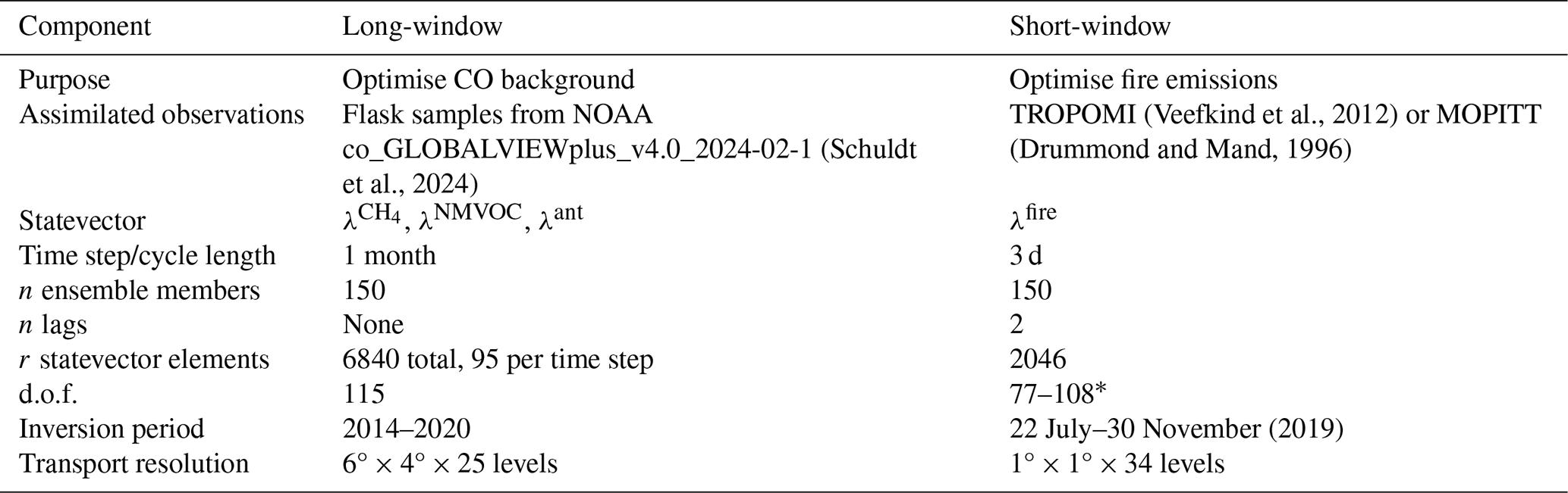
^* d.o.f. varies per short-window inversion cycle due to our emission-dependent covariance pre-masking (Sect. 2.4)

2.2 Prior fire emissions from GFED5.1 and GFAS v1.2

We start our inversions from two distinct fire emission inventories: GFED5.1 (van der Werf et al., 2025) and the GFAS v1.2 (Kaiser et al., 2012). Burned area-based inventories, such as GFED (van der Werf et al., 2017), calculate emissions by combining satellite-based burned area with biogeochemical model outputs and emission factors. The new GFED5.1 inventory has improved detection of small fires by including higher-resolution burned area inputs from Chen et al. (2023) based on corrections derived mostly from Sentinel-2 and Landsat. Globally, this nearly doubled burned area estimates relative to MODIS alone. For Brazil this resulted in a 61 % increase for 2019, particularly during the late dry season (July–October).

GFAS uses satellite-derived FRP observed by MODIS (both Terra and Aqua), to calculate fire emissions. Biome-level scaling factors based on GFED3 are used to convert fire radiative energy (FRE) to total dry matter burned (Heil et al., 2010), which are then combined with emissions factors that vary between biomes, mostly from Andreae and Merlet (2001), to calculate fire emissions.

All inventories use emission factors to convert total dry matter burned to trace gas emissions. Traditionally, these factors have been static biome averages while in reality they depend on fuel type, fuel moisture content, and meteorological conditions (van Leeuwen et al., 2013). Recently, Vernooij et al. (2023) combined a large set of savanna fire emission factor measurements across the world with geospatial proxies for these conditions (e.g. tree cover fraction, soil moisture, vapour pressure deficit) and a machine learning algorithm to derive dynamic savanna fire emission factors. GFED5.1 is the first inventory to operationally introduce spatio-temporal dynamic emission factors for savanna fires that allow a more realistic representation of temporal and regional variability.

GFED5.1 and GFAS v1.2 yield considerably different emission estimates for the 2019 fire season in Brazil of 41 and 25 TgCO, respectively. Expressed as total carbon, this difference translates to a factor of roughly 1.5. At the biome scale, the contrasts become even more pronounced. In the Amazon biome, for example, the two inventories differ by up to a factor of two in both their CO and total carbon emissions. Beyond underscoring the need for observations, these differences provide a means to assess the robustness of our inversions by examining how the optimised emissions respond to each prior.

2.3 Atmospheric transport and chemistry

We use the Transport Model 5 Massive-Parallel (TM5-MP; Krol et al., 2005; Williams et al., 2017) model to transport the CO emissions and production fields, from which vertical profiles of CO mole fractions and pressure are sampled. These profiles, combined with averaging kernels, are subsequently used in CTDAS to derive X_CO.

The short-window TM5 simulations were performed globally at a horizontal resolution of 1° × 1°, with 34 vertical levels, driven by three-hourly meteorological fields from the European Centre for Medium-Range Weather Forecasts (ECMWF) Reanalysis v5 (ERA5; Hersbach et al., 2020). Dry deposition is computed online. CO chemistry is linearised by prescribing three-hourly OH fields from the Copernicus Atmosphere Monitoring Service (CAMS) ECMWF Atmospheric Composition Reanalysis 4 (EAC4) dataset (Copernicus Atmosphere Monitoring Service, 2020; Inness et al., 2019), as well as the CO production from CH₄ and NMVOC oxidation optimised by the long-window. Fire emissions are distributed vertically using injection heights from the IS4FIRES dataset (Sofiev et al., 2012, 2013).

2.4 Statevector, covariance structure, and state propagation of the short-window system

Each statevector element (r) in ${\mathit{\lambda }}_{r,t}^{\mathrm{fire}}$ from Eq. (1) represents a 1°×1° grid box over land in South America between 22.5° S, 9.5° N, 79.5° W, and 34.5° W, resulting in a total of 1023 spatial unknowns (Fig. 1). At the start of each 3 d cycle, ${\mathit{\lambda }}_r^{\mathrm{fire}}$ are set to 1.0. We run the SW system with a 3 d assimilation window and 2 lags (i.e. 3 d lag). The scaling factors are optimised with a square root ensemble Kalman Smoother (Whitaker and Hamill, 2002; Peters et al., 2005). We minimise the cost-function equation as defined in Peters et al. (2005). In each cycle, a total of (2×1023) optimised scaling factors are thus calculated in the SW inversion. The optimised mean state of each cycle is propagated to inform the next cycle's mean state. This mean state is determined as the average between the current cycle's optimised state and a state filled with λ values of 1.0 (which represent the prior fluxes that are calculated by the long-window system). This procedure ensures that the scaling factors quickly revert back to the unscaled prior value of 1.0 when no CO observations are present.

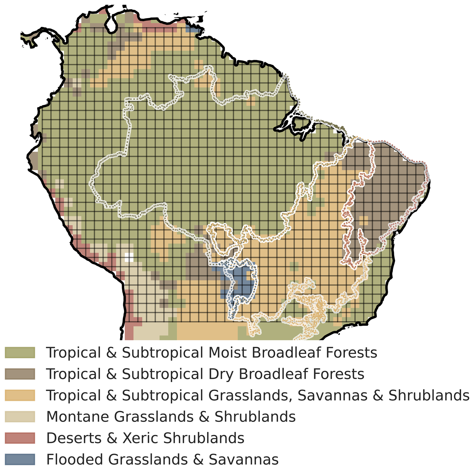
Figure 1 Region of interest for the short-window inversion. Grid lines indicate the spatial definition of the short-window statevector. Background colours show the biogeographic biome classification of Dinerstein et al. (2017) (a revision of the map by Olson et al., 2001), courtesy of the World Wide Fund for Nature (WWF), which we use to structure the prior covariance matrix. Overlaid outlines show biome boundaries from the TerraBrasilis platform, courtesy of the Instituto Nacional de Pesquisas Espaciais (INPE) (TerraBrasilis, 2025), which we later use to analyse fire emissions.

The degree of uncertainty on each scaling factor and their spatial correlations are described by the prior covariance structure. This covariance structure reflects our assumption that the errors in emission inventories are related to emissions factors and fuel characteristics or conditions, which often have some biome-dependency. We set the prior uncertainty to 100 % of the prior emission (variance = 1.0) and impose spatial correlations within biogeographical biomes using an e-folding distance correlation of 300 km (see also Fig. 1). Note that our inversion system is not designed to resolve emissions from individual fire plumes, a.o. due to the 1° × 1° resolution of our transport model and scaling factors, as well as biome level error correlations. Instead, it provides top-down constraints on fire emissions at the aggregated biome level.

Given that only a subset of the gridded fire emission state contains non-zero values within a 3 d cycle, we restrict the state-space to these active grid cells. This targeted state reduction mitigates the impact of zero-signal elements, which can otherwise dilute the ensemble covariance estimate.

Fire emissions are inherently non-negative and represent a bounded quantity. However, in practice, the optimisation algorithm may generate negative λ values that correspond to physically impossible negative emissions. We apply a semi-exponential transformation (Eq. 2), similar to Bergamaschi et al. (2009), to the optimized scaling factors where λ<1.0. We acknowledge that this transformation introduces non-linearity in the relationship between the statevector deviations and X_CO deviations (x^′ and ℋ(x^′) respectively, see Peters et al., 2005), yet we consider the use of the transformation to be more physically consistent, as it ensures the exclusion of unrealistic negative emissions. Besides, because we run a lagged system, subsequent lags can compensate for any non-linear effects introduced by this transformation.

$$\begin{array}{}\text{(2)}& \mathit{\lambda }=e^{(\mathit{\lambda }-\mathrm{1})}\text{for}\mathit{\lambda }<\mathrm{1}\end{array}$$

2.5 Observations for assimilation or validation

2.5.1 S5P-TROPOMI

The TROPOspheric Monitoring Instrument (TROPOMI) is a push-broom imaging spectrometer that measures backscattered solar radiances in the near-infrared (675–775 nm; NIR) and shortwave–infrared (2305–2385 nm; SWIR) (Veefkind et al., 2012). CO columns are retrieved using the shortwave infrared CO retrieval algorithm (SICOR Landgraf et al., 2016). The instrument is mounted on the Sentinel 5 Precursor (S5P) satellite. S5P was launched on 13 October 2017 and flies in a sun-synchronous polar orbit at 824 km, crossing the equator at 13:30 LST. Due to its wide swath (2600 km across track), TROPOMI X_CO data covers Amazonia daily. At nadir, the columns have a footprint of 7×7 km² (before) or 5.5×7 km² (after) 6 August 2019.

TROPOMI X_CO has extensively been validated against TCCON ground-based measurements and shown to meet the mission requirements of 10 % precision and 15 % accuracy (Borsdorff et al., 2018; Sha et al., 2021). Borsdorff et al. (2018) reported that, for clear-sky retrievals over land, biases are 6±4 ppb, while Sha et al. (2021) found that, with recommended quality filtering, X_CO biases average 9±3 % across most TCCON stations. In addition, Martínez-Alonso et al. (2022) compared TROPOMI with the MOPITT archive and demonstrated close agreement, particularly over land, with a mean difference of $-\mathrm{3}\pm \mathrm{11}$ % relative to the MOPITT TIR product.

We use the L2 RPRO v2 product, downloaded from the Non Time Critical (NTC) stream in the Copernicus data space. We only include retrievals with a quality control flag of flag > 0.5 as recommended by Apituley et al. (2024). The applied quality filter excludes observations under a range of potentially problematic cloud and aerosol conditions, although residual biases in dense smoke plumes cannot be completely ruled out. To allow for a “fair” comparison between the high-resolution TROPOMI retrievals and our coarser 1°×1° transport resolution, we generate 0.5°×0.5° superobservations following Rijsdijk et al. (2025).

2.5.2 Terra-MOPITT

The Measurement of Pollution in the Troposphere (MOPITT) instrument is a gas-correlation radiometer onboard the NASA Terra satellite (Drummond and Mand, 1996). Terra flies a sun-synchronous orbit at 705 km. At nadir, MOPITT has a spatial resolution of about 22 km² and overpasses at approximately 10:30 a.m. and p.m. local time. Launched already in 1999 (18 December), MOPITT remained active until recently (9 April 2025), delivering a long valuable data record (Canadian Space Agency, 2025). We use the L2 version 9 thermal-infrared (TIR; 4.7 µm band) retrieval product (Deeter et al., 2003, 2022) and exclusively assimilate daytime overpasses. The vertical sensitivity of the MOPITT TIR product (mid-troposphere) is different and complementary to TROPOMI (sensitivity almost uniform throughout the troposphere). The reliability of MOPITT retrievals has been well documented (e.g. Worden et al., 2010; Deeter et al., 2022), with retrieval biases for the version 9 TIR-only data stream estimated to be approximately 5 %. The recent implementation of an enhanced cloud detection algorithm in the version 9 product has improved both the coverage and sampling frequency compared to version 8 (Deeter et al., 2022). This particularly benefits regions like the Amazon.

Note that the MOPITT record has a data gap between 26 June and 24 August 2019 resulting from instrument failure and subsequent decontamination and hot calibration procedures (NCAR, 2024). This period covers substantial CO emissions according to the bottom-up emissions, which consequently remain unchanged in our inversion when assimilating X_CO from MOPITT.

Naus et al. (2022) demonstrated that the TIR product places strong constraints on fire emissions in the Amazon. Alongside the TIR product, MOPITT provides a near-infrared and thermal-infrared (NIR+TIR) product. The NIR product is limited to daytime data and is more sensitive to CO mole fractions in the lower troposphere compared to the TIR product (Deeter et al., 2022). Past CO inversion studies have employed both products, though not simultaneously (e.g. Nechita-Banda et al., 2018; Naus et al., 2022; Peiro et al., 2022).

2.5.3 Ground-based and aircraft observations

The simulations are evaluated against independent in-situ CO measurements from the Atmospheric Tall Tower Observatory (ATTO) site in central Amazonia (Lavric and Walter, 2019). We calculated hourly averages from the 2019 record on the 80 m walk-up tower (2.14° S, 59.00° W). The samples were measured with a Picarro G1302 (CKADS-18) cavity ring-down spectrometer. We converted the data from the WMO X2004 to the WMO X2014A calibration scale. These tower data are used only for evaluation, not assimilation.

We also use aircraft vertical profile measurements from the Obspack collection obspack_multi-species_1_manaus_profiles-_v2.0_2023-09-26 (Miller et al., 2023). The profiles sample the troposphere approximately 80 km north-east of Manaus. In total, nine flights were taken during our study period (22 July–30 November 2019) with descending vertical extents between 5850 to 250 m (above sea level). The profiles were measured using a Picarro G2401-m (Miller et al., 2023).

We sample TM5 at the location of each individual sample in the tower and aircraft data series using three-dimensional interpolation and hourly averages centred around the measurement time.

2.5.4 Model data mismatch and data selection

The observation error in the cost function usually consists of the actual instrument error (or retrieval/super-observation error) and a representativeness-error estimate of the transport model (i.e. model–data-mismatch error). We determine the latter error contribution following Basu et al. (2018) in which the representativeness error is proportional to the simulated column gradient at a given location with its neighbouring grid boxes. The total model–data mismatch is then taken as the quadratic sum of the instrument and representativeness-error components. To assess whether our assumed error statistics are consistent with the actual model–observation differences, we use the innovation χ², defined as:

$$\begin{array}{}\text{(3)}& {\mathit{\chi }}_{\mathrm{inno}}^{\mathrm{2}}={\displaystyle \frac{(y-\mathcal{H}(x){)}^{\mathrm{2}}}{(H{P}_t^b{H}^T+R)}}\end{array}$$

where y is the observation, ℋ(x) the model equivalent of the observation, $P_t^b$ the prior error covariance and R the observation error covariance or model-data-mismatch. A ${\mathit{\chi }}_{\mathrm{inno}}^{\mathrm{2}}$ close to one indicates that the actual residuals are in balance with the expected uncertainties.

The total errors associated with TROPOMI super-observations are generally smaller than the uncertainties that characterise individual MOPITT X_CO retrievals (∼ 3 ppb vs. ∼ 7 ppb on average for all X_CO). To ensure that the innovations are neither systematically over- nor under-weighted in the cost function – we increased the model–data-mismatch error by doubling the transport-error component and adding a fixed 4 ppb term. This adjustment reflects our expectation that TM5 has greater difficulty with boundary-layer transport (where TROPOMI is more sensitive than MOPITT) than to free-tropospheric transport (where MOPITT's sensitivity peaks). It also compensates for a likely underestimation of systematic errors in the super-observations and any unaccounted-for error correlations between individual retrievals. After inflation, the bulk of the ${\mathit{\chi }}_{\mathrm{inno}}^{\mathrm{2}}$ approached one (mean 3.75; median 1.51), indicating a well-balanced and statistically consistent error characterisation.

As our statevector only contains scaling factors for fire emissions, we preselected observations for assimilation. The inversion only considers cases where either the observed or simulated (prior) X_CO was recently influenced by fires. We achieve this by applying a condition where either for the observed or modelled X_CO ≥ 125 ppb. To assess the robustness of this cut-off, we performed sensitivity tests using thresholds of 100 and 150 ppb. These showed that the derived total fire emissions were barely affected by the exact threshold choice (a spread of 1.1 TgCO, or 2 %–3 %, on Brazil fire season totals), suggesting that the information content relevant to the regional emission budget is concentrated in observations associated with strong CO enhancements. In addition, we verified that this targeted selection for higher X_CO did not result in strong CO accumulation in the background (simulated X_CO < 125 ppb; Appendix A2) which demonstrates that the threshold does not systematically bias our fire emission estimates.

Finally, X_CO samples with residuals exceeding three times the model–data mismatch (indicative of poor transport model performance in capturing observed fire impacts) are rejected for assimilation. We also exclude X_CO samples with reported surface pressure below 900 hPa, as such conditions (e.g. the Andes) are challenging for TM5 to model.

2.6 Inversion procedure

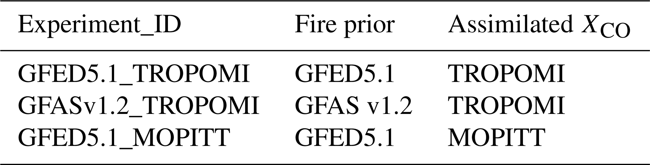
We conducted a series of inversion experiments to quantify Brazilian fire emissions and to assess the robustness of the estimates. These experiments test the sensitivity of the inversion results to the choice of prior fire emission inventory and the assimilated satellite instrument. The different configurations are summarised in Table 2.

In addition to testing the sensitivity to different priors and observational constraints, we quantified how uncertainties in OH chemistry and in CO production from NMVOC oxidation influence the inferred fire emissions. Rather than performing a new suite of inversions, we base this on a set of sensitivity experiments that was targeted to do this for the same region and for four fire seasons, by Naus et al. (2022) (see their Fig. S2). Naus et al. (2022) ran their inversions with two sets of OH fields, and two sets of chemical production fields. For each season that Naus et al. (2022) ran the experiments, we calculate the ensemble standard deviation across their sensitivity experiments and then average these values over all four years. This approach yields an estimated structural uncertainty of 15 TgCO per season in the posterior fire emissions. We consider this estimate conservative for two reasons: (1) their inversion domain extends beyond Brazil, whereas our reported emissions are limited to the Brazilian portion of the domain, and (2) our system includes an intermediate long-window inversion step.

Table 2 Inversion experiments overview.

3 Results

3.1 Comparison against observations

In this section, we demonstrate the performance of our inversions by comparing against observations. We start with a comparison to satellite-based X_CO and compare to surface observations (in-situ and aircraft). We focus these comparisons on our “base inversion” which started from GFED5.1 and assimilated TROPOMI superobservations.

3.1.1 TROPOMI and MOPITT

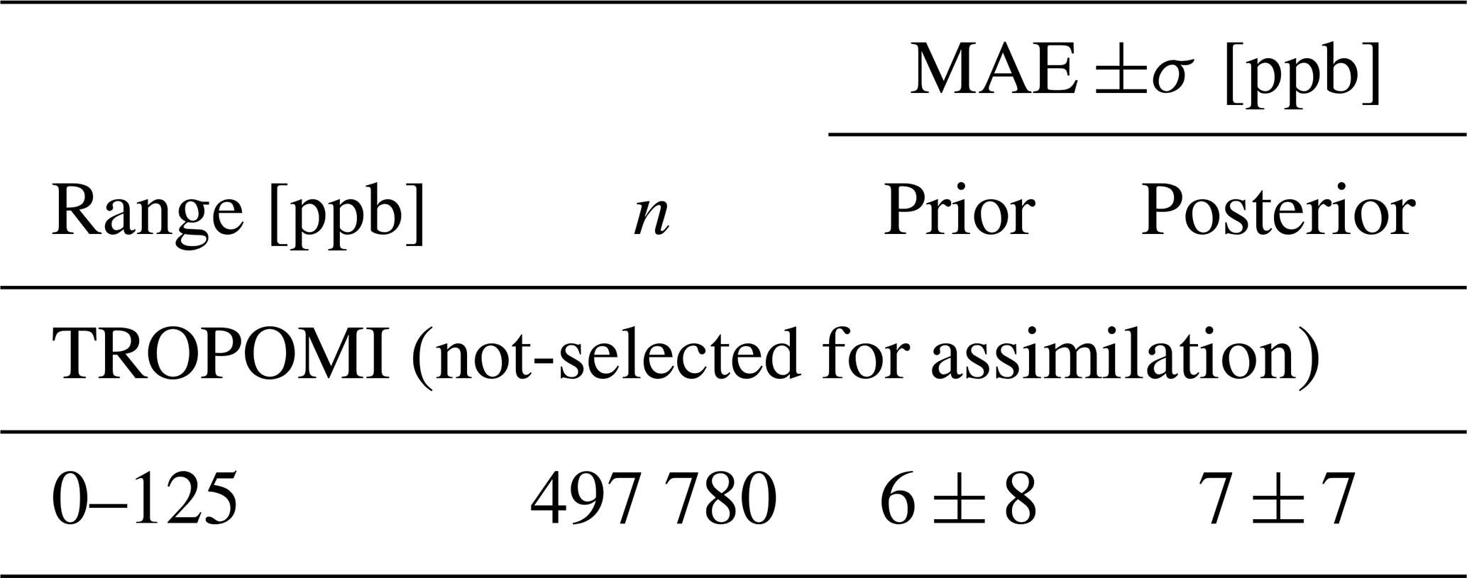
The short-window posterior consistently improves agreement with observations compared to the prior. When compared to assimilated TROPOMI data, the simulated and observed X_CO compare well, as expected (Fig. 2d–e, and Table 3). This improvement is most pronounced for elevated X_CO (> 125 ppb), where the mean absolute error is reduced by 42 %–55 %, with the strongest error reduction (∼ 17 ppb) for large X_CO (> 225 ppb) that are most representative of fire plumes.

Importantly, this improvement is not limited to assimilated data: validation against independent MOPITT observations also confirm closer alignment between simulated and observed CO (Table 3). The overall improvement in model–data agreement demonstrates that the short-window inversion effectively extracts information from the satellite retrievals.

In terms of spatial structure, the prior residuals are dominated by plume-shaped patterns associated with fire signals (Fig. 2f). The short-window inversion system effectively corrects most biases through adjustments to fire emissions (Fig. 2g). In an exemplary three-day cycle, TROPOMI observations show a plume stretching from north to south on the western flank of the basin (Fig. 2b) that is overestimated or displaced in the prior (Fig. 2f). Furthermore, plume structures south-east of the arc of deforestation are visible, which are strongly underestimated in the prior (Fig. 2f). The inversion corrects much of both discrepancies and substantially reduces biases in plume-dominated regions. Some mismatches remain – for example, the larger than 20 ppb underestimation in the southeastern Cerrado requires emission increases that introduce positive biases at more local scales in the northeastern Cerrado – but overall, the posterior provides the statistically best fit achievable within observational constraints and prior uncertainties.

The inversion also improves the temporal evolution of X_CO as confirmed by the Hovmöller diagrams with daily TROPOMI X_CO (Fig. 2c–e). The prior already reproduces broad seasonal variability, but negative biases emerge during the burning season: over the southwestern Cerrado-box (B3), where CO is strongly underestimated from mid-August to October, while the southeastern Amazon-box (B4) shows more rapid variations in the X_CO residuals. Note that for both boxes the negative residuals often are synchronous with increases in TROPOMI X_CO, indicative of fire episodes. The posterior reduces these residuals throughout most fire episodes.

Table 3 and Fig. 2d, e, f and g (boxes B3, B4) show that in the background-dominated air masses, X_CO barely changes and does not deteriorate after the inversion. This shows that our data selection threshold and scaling factor transformation choices did not lead to strong CO accumulation in the background. Together, these outcomes suggest that the short-window prior residual structure is mostly related to fires that the short-window inversion effectively targets by optimising to GFED5.1 bottom-up emissions.

Table 3 Mean absolute error (or residual) and the standard deviation of the residuals per observed X_CO bin for the GFED5.1_TROPOMI base inversion.

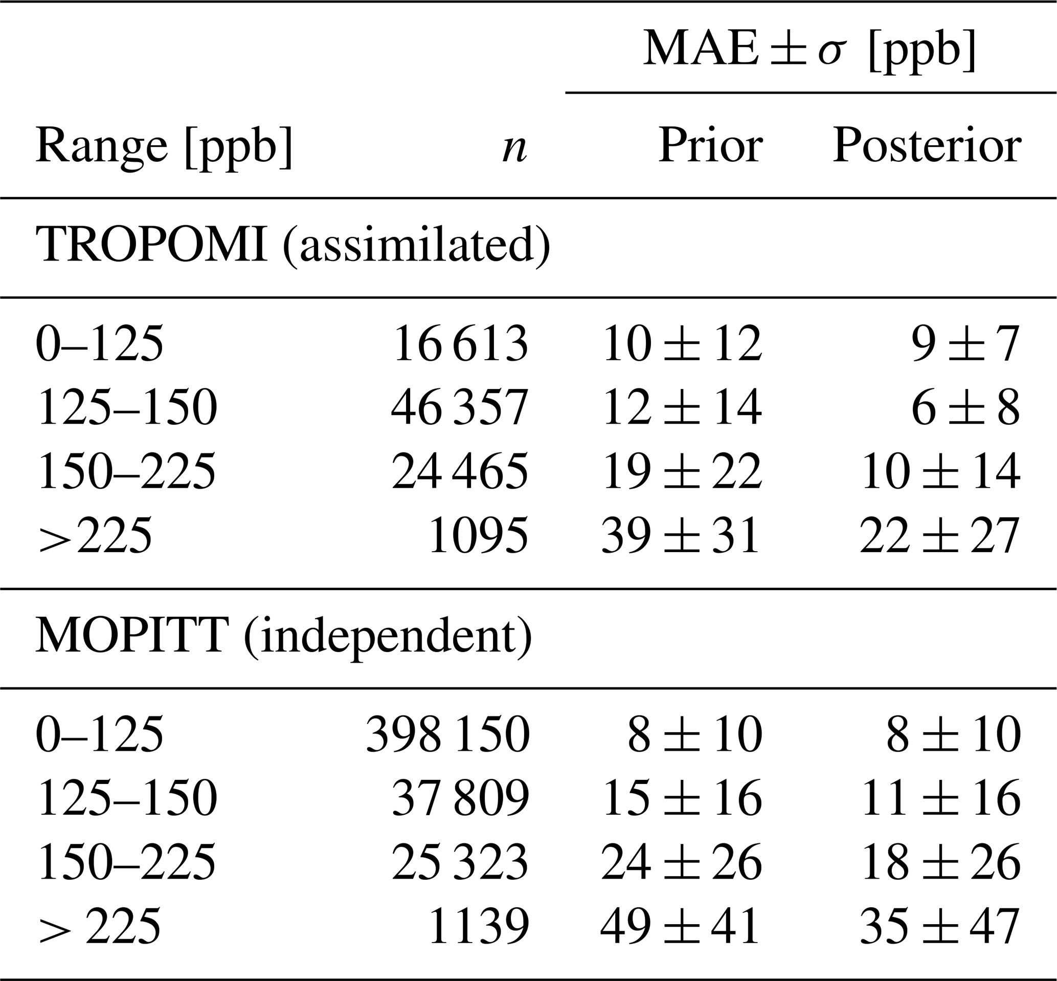
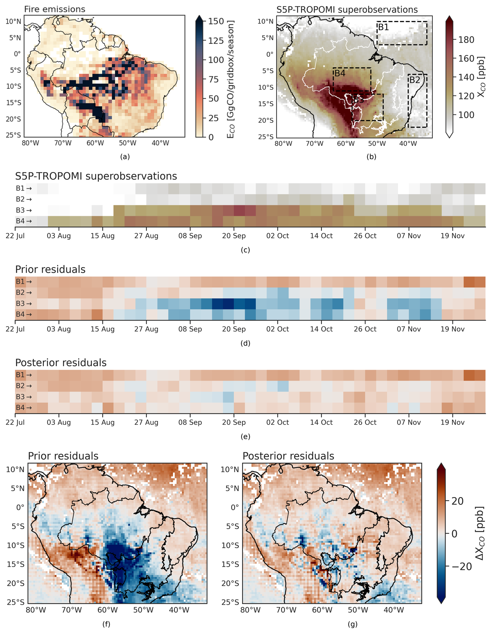
Figure 2 Evaluation of the GFED5.1_TROPOMI base inversion with S5P-TROPOMI superobservations. (a) Cumulative GFED5.1 prior emissions for the simulation period at 1°×1°. (b) TROPOMI X_CO averaged to a 0.5°×0.5° grid for an example 3 d period (14–17 September 2019) alongside corresponding (f) prior and (g) posterior residuals. (c) Hovmöller diagram of 3 d mean X_CO over the subregions indicated in (b): oceanic background (B1, B2), Cerrado (B3), and Amazon (B4); and (d, e) related prior and posterior residuals. Colour bars are shared between (b), (c) and (d)–(g).

3.1.2 Comparison to in-situ and aircraft observations

While the ATTO measurements do not sample intense fire plumes, they provide valuable independent information to validate background and moderate pollution levels inside the Amazon. Comparison against ATTO CO mole fractions (Fig. 3) demonstrates that the short-window posterior generally reproduces observed CO mole fractions well, with a mean absolute percentage error of 12 % over the 2019 fire season. This level of agreement with independent data provides confidence in the inversions. Note that the difference between the long-window and short-window posteriors reflects the combined changes of increased transport model resolution and fire emission optimisation. The narrow ensemble spread (shading around the lines; nearly invisible) represents the limited sensitivity in both the long- and short-window inversions at this site.

Although the short-window inversion yields improved validation scores for most cycles (Fig. 3), from time to time, deviations from this pattern are to be expected for a non-assimilated site, and they underline the importance of aggregating posterior results before interpretation. In particular, we find a local reduction in performance in the last cycle which can be attributed to Ensemble Kalman Smoother (EnKS) edge effects, where the final cycle is constrained by only a limited set of observations. When combined with state propagation and a poorly represented fire in close proximity to the ATTO site, this can affect performance metrics at a local scale. However, the influence of these edge effects on domain total emissions remains minimal, as is evident from Fig. 5.

We also evaluate the inversions against independent aircraft CO profiles collected near Manaus (Appendix A3). Compared to the long-window, the short-window inversion provides a clear improvement near the surface in the lower troposphere. The short-window posterior yields a mean absolute percentage error of 19 % relative to the observations. Although the short-window tends to better represent the profiles than the long-window inversion, much variability remains across individual profiles. Above 4 km, however, we keep a large positive residual (usually > 20 ppb) for all simulations, which we discuss in more detail in Appendix A3.

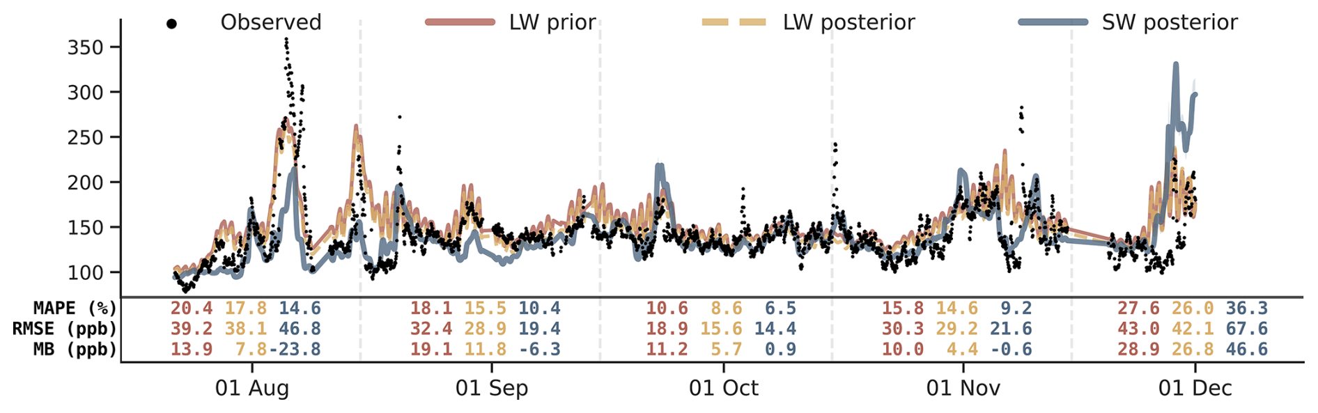
Figure 3 Measured and simulated CO mole fractions at the ATTO tower at 79 m a.g.l. measurement height. Lines show the long-window prior (red), long-window posterior (yellow), and short-window posterior (blue), with shading indicating one ensemble standard deviation from the mean. The short-window posterior is derived from the GFED5.1_TROPOMI inversion. Monthly validation metrics – mean absolute percentage error (MAPE), root mean squared error (RMSE), and mean bias (MB) – are reported in the corresponding colours for each run.

3.2 Brazilian fire CO emissions during the 2019 fire season

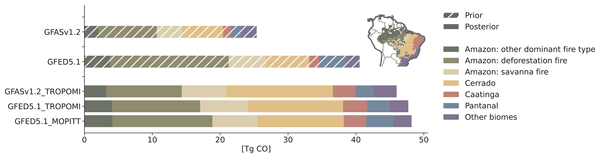
According to the GFAS v1.2 and GFED5.1 inventories, total CO emissions from fires in Brazil during the 2019 fire season (22 July–30 November) were 25 and 41 TgCO, respectively, as indicated in Fig. 4. Our inversions suggest that fire emissions are 47${}_{\mathrm{46}}^{\mathrm{48}}$ TgCO (mean${}_{\min }^{\max }$). The posterior emissions deviate by less than 20 % from the GFED5.1 prior. For GFAS v1.2 however, the inversions imply that an 81 % increase of emissions is needed. This prior-posterior increase is substantially higher than the average 50 % increase that Naus et al. (2022) found for the 2003–2018 fire seasons and will be discussed in more detail (Sect. 4).

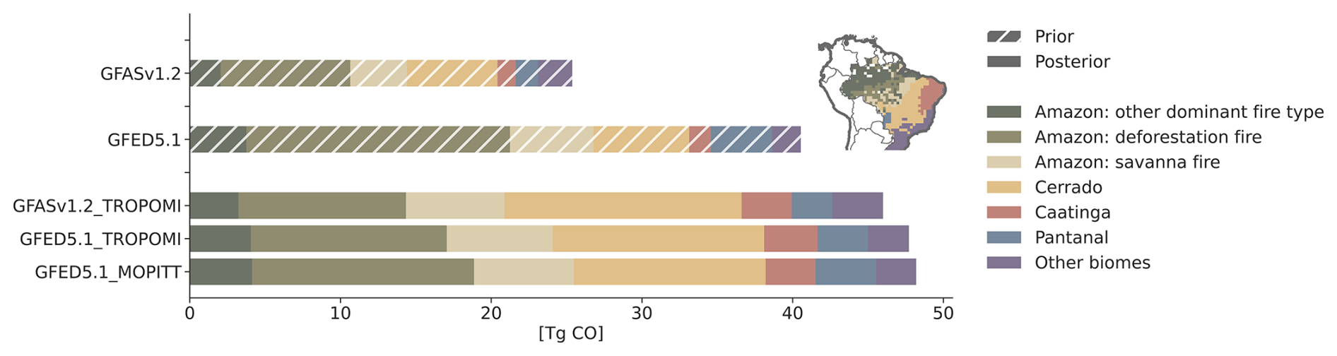
Figure 4 Prior and posterior CO fire emissions [TgCO] for the 2019 Brazilian fire season. Coloured stacked bars represent contributions from different biomes. Emissions in the Amazon biome have been disaggregated to dominant fire types based on Andela et al. (2022).

Despite starting from substantially different prior fire-emission totals, the inversions converge to nearly the same posterior fire-emission integral over the season (46.0 and 47.7 TgCO). Likewise, inversions that assimilate either TROPOMI or MOPITT data end up with similar fire season totals (47.7 and 48.2 TgCO), underscoring the robustness of the posterior estimates to both the choice of prior and the choice of satellite instrument.

On more local scales (bar-stacks in Fig. 4) or shorter time intervals, the posterior emission spread becomes larger in a relative sense but still demonstrates strong convergence from multiple priors and instruments down to 3 d intervals for most periods analysed (Fig. 5).

3.3 Biome-level fire emissions and their temporal variation

To better understand the origin and dynamics of posterior–prior differences, we analyse CO emissions at the biome level and their temporal evolution. Given the contrasting fire dynamics and the shifting position of the arc of deforestation relative to biome boundaries, we further subdivided the Amazon emissions into the season’s dominant fire types following Andela and Jones (2024). As shown in Figs. 4 and 5, savanna fires make a substantial contribution within the Amazon biome (21 %–32 %), and their temporal evolution aligns more closely with Cerrado fires than with deforestation events, supporting this subdivision.

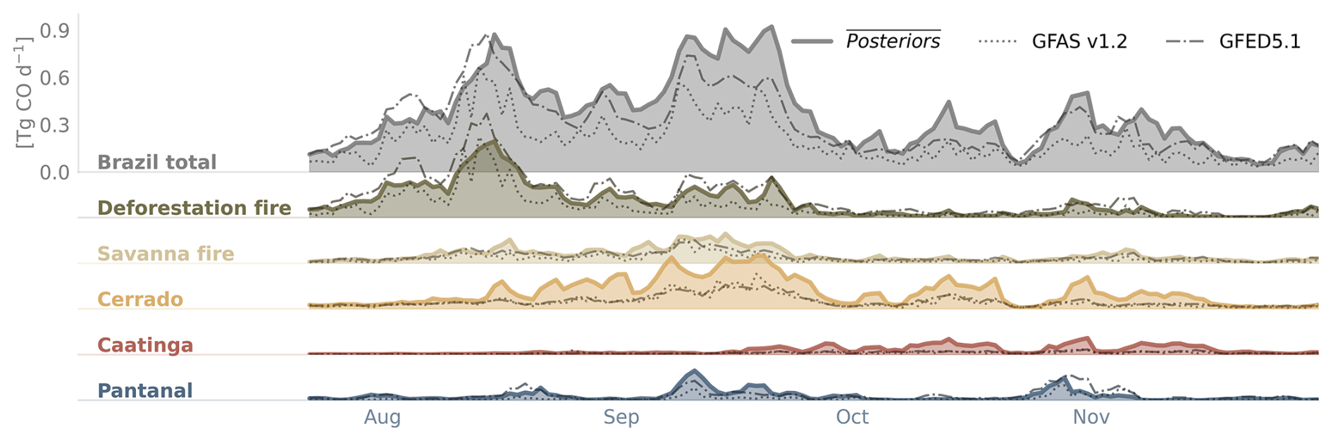
Figure 5 Daily evolution of CO fire emissions by biome. Filled areas and thick lines show the posterior mean across the three inversions (GFED5.1_TROPOMI, GFED5.1_MOPITT, and GFASv1.2_TROPOMI), while dashed lines indicate corresponding priors (– ⋅ – GFED5.1, ⋯ GFAS v1.2). The y-axis is shared across all biomes for direct comparison; successive ridges are spaced at 0.3 TgCO d⁻¹ intervals and can serve as visual reference marks. The posterior spread can be found in Fig. A4.

The temporal evolution of fire CO emissions during the 2019 dry season is characterised by a clear succession of different fire regimes (Fig. 5). Both prior and posterior estimates reproduce this phasing, but the posterior estimates highlight important discrepancies in the magnitude of emissions for several biomes – most notably the Caatinga and Cerrado, where optimised emissions differ by a factor of 2–3 from their priors. Figure 5 illustrates this evolution, which we divide into three phases: early-season (mid-August), mid-season (mid-September), and a widespread late-season tail (October–November).

3.3.1 Early season (mid-August)

The early 2019 fire season was dominated by fires in the Amazon biome, with emissions primarily from deforestation and forest fires linked with coarse woody fuels that burn mostly in the smouldering phase. This peak was abnormally early compared to the 15-year preceding GFAS v1.2 and GFED5.1 means (not shown). In this period, priors disagree most: GFAS v1.2 estimates are sometimes up to three times lower than GFED5.1 during the period until late August, adding up to 6.1 TgCO vs. 11.4 TgCO respectively. Meanwhile, the posterior mean estimate falls in between (8.8 TgCO). We note that this period also shows the largest spread in posterior estimates (Fig. A4; adding up to a range of 20.9–25.5 TgCO over the full season). This spread is driven by the absence of observational constraints from MOPITT during most of August (Sect. 2.5.1), while TROPOMI inversions lean towards GFAS v1.2. Including this unconstrained period into our final multi-inversion posterior mean pulls the ensemble mean estimate toward the GFED5.1 baseline by up to 2.7 TgCO (difference between GFED5.1 and the mean of the two inventories for this period). Furthermore, TROPOMI inversions suggest a minor shift in CO emissions from deforestation to savanna-type fires in the Amazon and Cerrado regions. The mid-august peak in both priors remains preserved, however there seems to be a timing shift of 1–2 d, which may be related to our use of 3-daily (and not daily) scaling factors.

3.3.2 Mid-season (mid-September)

During September, fire activity shifts decisively toward the Cerrado. These fires are characterised mostly by fast-burning, flaming combustion with low CO emission factors (61 gCO kgDM⁻¹ in GFAS v1.2 and Fig. A5 for GFED5.1). In contrast to the deforestation fires in the early season, the priors are in much closer agreement here. Regardless, the posteriors consistently indicate that an upward adjustment, of often more than two times the prior, is required to agree with MOPITT and TROPOMI observations, reflecting the strongest emission modifications in the inversions. This could suggest that prior inventories underestimate Cerrado fire emissions at the first seasonal peak (∼ 5 TgCO between mid-August and late September).

3.3.3 Late season (October–November)

The late fire season is characterised by a more heterogeneous mix of fire types across multiple biomes. Savanna fires in both the Amazon and Cerrado continue to contribute substantially, accounting for 45 % of Brazil’s total CO emissions in the prior and increases to roughly 65 % in the posterior between October and December. These savanna fires also persist well into late November. From late October onward, some residual burning remains in the Amazon biome, and additional activity emerges in the Pantanal wetlands, which typically requires prolonged dry conditions before they can sustain fire.

During October and November, the posterior mean estimate for Brazil (13.3 TgCO) indicates that emissions remain considerably higher than suggested by the prior inventories (6.4 TgCO in GFAS v1.2 and 10.9 TgCO in GFED5.1), with the most notable increases in the Caatinga and Cerrado regions.

4 Discussion

Our study provides a satellite-constrained estimate of CO fire emissions for the 2019 Brazilian fire season. The convergence of our inversions based on independent X_CO from TROPOMI or MOPITT and fire inventories on a total of 46–48 TgCO underscores the robustness of the top-down estimates and highlights the value of satellite instruments to constrain the magnitude of Brazilian fire emissions. This estimate comes with an uncertainty estimate of ∼ 15 TgCO that represents structural knowledge gaps concerning CO production from the oxidation of NMVOCs and loss by OH. Our study also serves as a cross-validation of the two satellite datasets, and the convergence of posteriors shows potential for combined use of the instruments to explore their constraints on the vertical distribution of CO in future research.

4.1 Comparison with prior fire emission inventories

When comparing our inversion results with existing bottom-up inventories, we find encouraging progress in fire emission modelling. This is demonstrated by the good agreement with the new GFED5.1 dataset (posterior within < 20 % of GFED5.1), as opposed to the older GFAS v1.2 product (posterior deviates > 80 %). The agreement with GFED5.1 suggests that recent updates, such as the inclusion of the new small-fire burned area dataset, help to better capture regional fire regimes.

When analysed at biome level, the inversion suggests large fire emission changes for fires in the Amazon, ranging between 3–9 TgCO, with a reduction and increment compared to GFED5.1 and GFAS v1.2 respectively. However, the posterior mean (23.5 TgCO) ends up well within the large prior range of 14.3–26.8 TgCO as inventories in tropical forest regions remain uncertain. Detection of emissions from understory fires remains inherently challenging due to persistent cloud cover and dense canopies (Morton et al., 2013). It should be acknowledged that our posterior spread remains relatively large for this region (20.9–25.5 TgCO) in part due to limited observational constraints from MOPITT during the peak of the fire season here and that our system has limited capacity to account for a lack of emissions due to missed detections, as will be discussed later.

In contrast, we find systematic emission increments for the Cerrado and the Caatinga biomes. The inversion adjusts the prior by a factor two, resulting in a 7–8 TgCO prior-posterior gap. This result is unexpected, as fire dynamics in these savanna-dominated ecosystems are typically considered relatively well captured and constrained by global inventories due to availability of ground measurements and relatively straightforward fire dynamics. Our findings however, are in line with previous work by Naus et al. (2022), who also reported a systematic underestimation of savanna and shrubland fire emissions by GFAS v1.2. In their work the median difference between the prior and posterior emissions also approached a factor of two, while using a different inversion algorithm (4D-var v. EnKS), meteorological driver data (ERA-Interim v. ERA5), and different CO source/sink datasets. The remainder of this discussion will investigate the potential drivers of this large and systematic discrepancy between our inverse results and the fire inventories.

4.2 Potential drivers of the Cerrado/Caatinga emission gap

To understand the source of the discrepancy between the prior and posterior Cerrado/Caatinga emissions, we first assess potential errors in our inversion framework before discussing the prior inventories.

First, transport modelling errors can play a role. The comparison of TM5 simulated vertical profiles of CO against observed CO from aircraft flights near Manaus suggest that convective mixing of surface signals aloft is too strong in TM5 (Fig. A2). At the same time, major errors in vertical transport seem unlikely given the strong consistency between TROPOMI- and MOPITT-based inversions despite their different vertical sensitivities and overpass times. Nonetheless, transport modelling errors remain a source of uncertainty in atmospheric inversions. These uncertainties are challenging to quantify and would benefit from for instance an inter-comparison study with different transport models over South America, which is beyond the scope of this work.

Second, Lichtig et al. (2024) showed that African fires contribute up to 25 % of tropospheric CO mass over eastern Brazil. The good agreement between TROPOMI observations and TM5 simulated fields over the main inflow regions (Sect. 3.1.1, B2 in Fig. 2d) suggests, however, that long-range transport biases are small. Moreover, the good agreement negates the hypothesis that the high emissions are a compensation for a lack of CO inflow from distant fire emissions or CO production from CH₄ oxidation in the background atmosphere.

Third, weak correlations between the posterior Cerrado emission ensembles with other regions suggest that the inferred increments over the Cerrado are genuine local signals rather than the inversion compensating for omitted emissions in neighbouring biomes or countries (Appendix A6).

Fourth, localised chemical sources or sinks – such as CO production from NMVOC oxidation or loss through OH – remain an alternative explanation for the differences over the Cerrado and Caatinga. However, the magnitude of the sub-regional changes required makes this unlikely. To close the emission gap, NMVOC-derived CO production in these regions would need to increase two- to fourfold. Besides, this assumes a 1:1 compensation between NMVOC-CO and fire-CO, but as Naus et al. (2022) demonstrated, the relationship is closer to 2:1, implying an even larger and less plausible adjustment would be needed. Furthermore, such a large, localised change in the NMVOC source would require compensating biases elsewhere and degrade the current good agreement with independent CO budget estimates (Zheng et al., 2019; Naus et al., 2022).

Following the same reasoning, we think that large OH biases in the Cerrado/Caatinga are improbable. Moreover, the CAMS state-of-the-art chemical data assimilation system has constraints on species important for OH-chemistry through extensive assimilation of satellite observations, making such systematic biases in our imposed OH fields unlikely. Also, a recent inter-comparison by Jones et al. (2026) shows that CAMS EAC4 surface ozone (a key OH precursor) lies at the low end of current reanalyses, suggesting that EAC4 could more likely underestimate than overestimate OH. More OH in our inversion would, if anything, increase inferred fire emissions, further stretching the prior-posterior Cerrado/Caatinga emission gap.

While structural uncertainties in the representation of the chemical sources and sinks are substantial, ±15 TgCO (see Sect. 2.6), we argue that the current chemical source and sink terms cannot fully account for the Cerrado/Caatinga posterior estimates without degrading agreement with observations in downwind regions (e.g. Sect. 3.1.1). Therefore, the adjustment in the Cerrado/Caatinga seems to be plausible not only because it is independent of the data assimilated in our inversions, but also because it is consistent with other top-down studies that found larger CO and CO₂ emissions in the Cerrado and Caatinga biomes (Naus et al., 2022; Botía et al., 2025).

4.2.1 Global fire emission inventory perspective

In previous research, underestimation of fire emissions has often been linked to missing small fires (Ramo et al., 2021; Roteta et al., 2019; Randerson et al., 2012; Ouattara et al., 2025). Detection can be further limited where dense smoke or aerosol loading suppresses the thermal signal used in FRP-based active-fire retrievals (Cohen, 2014). Underestimations in burned area, however, have been substantially mitigated in GFED5.1 (Chen et al., 2023; van der Werf et al., 2025). Compared to the Amazon, the savannas of the Cerrado and Caatinga usually have less cloud cover and lower canopy density, which facilitates more reliable satellite-based fire detections. For these reasons, we expect undetected fires to contribute only marginally to the remaining prior-posterior discrepancy.

Second, uncertainties in CO emission factors (EFs) could contribute to the emission gap, but it is unlikely that they can explain the mismatch between bottom-up inventories and our top-down study entirely. Literature reported uncertainties in CO EFs for savanna fires are 28 %–30 % (Andreae and Merlet, 2001; Andreae, 2019) and the Cerrado/Caatinga average CO EFs in GFAS v1.2 and GFED5.1 are substantially different, with 65 g CO kg DM⁻¹ (dry matter) in GFAS v1.2 (Kaiser et al., 2012; Andreae and Merlet, 2001), while GFED5.1 approaches a region weighted average of 55 g CO kg⁻¹ dry matter when the majority of dry matter is combusted (Fig. A5). Taking this into consideration, a 20 % uncertainty in the prior EF appears reasonable. However, applying a 20 % increase to the prior emissions would only account for about 20 % of the ∼ 8 TgCO prior-posterior Cerrado/Caatinga emission gap. To close the gap entirely, the average EF for these savanna fires would need to exceed that of tropical forest fires (101–109 g CO kg DM⁻¹ (Andreae and Merlet, 2001; Andreae, 2019)), which is unrealistically high for savanna fires. Therefore, while EF uncertainties may be a contributing factor, they alone cannot resolve the factor-of-two discrepancy between our posterior estimates and the prior inventories.

A third possible source of underestimation lies in how the two inventories calculate total matter burned. Although GFAS v1.2 and GFED5.1 report similar total CO emissions for the Cerrado/Caatinga (7.2 and 7.8 TgCO, respectively), their substantially different CO EFs imply that their underlying total dry matter burned estimates are not in agreement. For GFAS v1.2, Eames et al. (2025) also found (total carbon) emissions to be on the low end for a savanna region in Africa and listed three potential reasons related to underestimated total matter burned that are relevant for the Cerrado/Caatinga region too: (A) GFAS is tuned to the older GFED (version 3) version that did not account for small fires, (B) use of a globally unified conversion factor from FRE to mass DM burned (kgDM MJ⁻¹) that may not be representative for all savanna types, and (C) weakening of the FRE signal by tree canopies in woody savannas.

Recent studies also support the hypothesis of underestimated fuel loads in GFED5.1. Forkel et al. (2025) demonstrated that the woody debris and litter estimates in GFED500m (Van Wees et al., 2022) are low for the Cerrado when compared to both field measurements and a GEDI LiDAR-based fuel map from Leite et al. (2022). This is particularly important because litter and coarse woody debris constitute over 90 % of the fuel in savanna fires within the Amazon and Cerrado biomes according to Forkel et al. (2025), underscoring the need for accurate characterisation of these fuel pools. Even minor shifts in fuel quantity can be significant if they coincide with shifts towards fuel types associated with higher CO EFs.

Accurate modelling of these fuel pools at a global scale remains a major challenge. As both Van Wees et al. (2022) and Eames et al. (2025) discuss, surface and below-canopy fuels are difficult to observe with satellites. Consequently, models often rely on empirical tuning. For instance, the GFED model's carbon pool turnover rates are tuned using data from field campaigns (Van Wees et al., 2022), which may not capture the full heterogeneity of the vast and diverse Cerrado/Caatinga region.

Finally, fire dynamics over the regions have been changing and it is unclear if global inventories represent this well. Our inversion indicates the largest emission adjustments in the northeastern Cerrado (MATOPIBA: Maranhão, Tocantins, Piauí, and Bahia) region, an area where most native vegetation remains, which are under strong pressure from human activities (Silva et al., 2021; Alencar et al., 2020). Over the past three decades, nearly half of the Cerrado's native vegetation has been converted to other land uses (Alencar et al., 2020), which could imply fundamental alterations in fire characteristics such as fuel type, load, and consumption, and consequently, emission factors that may not be adequately included in global inventories. While the years pre- and post land use conversion show increased fire activity, negative trends in burned area emerge as the converted lands age (Ribeiro et al., 2024). Human activities fragment the landscape, which can disrupt the natural cycle of frequent, low-intensity fires, leading to woody encroachment (Stevens et al., 2017; Rosan et al., 2019). This build-up of fuel increases the risk of larger and more intense fires (Fidelis et al., 2018). More woody fuels in turn usually are characterised by higher EFs. For example, provided that emission factors in inventories often are (at least in part) based on field measurements before the 2000's and static in time (e.g. Kaiser et al., 2012; Andreae and Merlet, 2001), such dynamics may not be represented through emissions factors.

4.3 Outlook and Future Directions

This study and our new modelling framework open the path for future research. For example, we want to highlight the potential of leveraging CO to improve fire detection and quantification, particularly for small and cloud- or canopy-obscured fires that traditional bottom-up methods may still under-represent. Although our current framework effectively constrains regional emissions, it has only limited capability to assign emissions locations where the priors have no or low emissions because the errors we assign to each location depend on the magnitude of the local fire emission itself. Future studies could build on our work by implementing more flexible prior error structures. For example, adopting approaches that allow the inversion to allocate emissions more freely, such as in Yin et al. (2015), could allow a more complete exploitation of downwind CO observations and refine emission estimates for low-intensity fire regimes.

Furthermore, our data selection strategy focused on fresh fire plumes by using a 125 ppb threshold, which proved effective in constraining peak fire emissions without introducing strong biases in CO background mole fractions. Future work should explore more dynamic data selection methods or consider assimilation of background X_CO in the long-window inversion step. Such advancements would allow for the assimilation of all available observations, which could help to capture more diffuse, widespread fire emissions that lead to lower yet detectable X_CO increases.

In addition, we acknowledge that our 3×R rejection strategy, while standard practice, may have led to the exclusion of some valid high-concentration observations. As a result, the most extreme fire enhancements that were simulated and not observed, or vice versa, may be partially filtered out. The prior residuals of these rejected samples do not suggest that we systematically under- or overestimate the posterior fire emissions. Nonetheless, we may have rejected some valid data and we recommend future studies to consider exploring more sophisticated, possibly non-Gaussian outlier detection methods that are better suited to process fire plumes.

Aerosol-induced X_CO retrieval biases are a potential concern in dense smoke plumes because aerosols modify the light path of photons which might affect retrieval sensitivity. However, aerosol scattering effects are explicitly accounted for in the SICOR retrieval and sensitivity tests presented in the algorithm theoretical baseline document that include cases with high aerosol loads, suggest the algorithm remains within 1 % uncertainty (Landgraf et al., 2024). In addition, a validation campaign during a wildfire suggests that uncertainties remain within mission performance requirements even in optically thick smoke plumes (10 % accuracy, 15 % precision) (Rowe et al., 2022). Aerosol radiative effects in the 4.7 µm thermal-infrared absorption band are weak (Eck et al., 1999) and therefore not explicitly accounted for in the retrieval (Francis et al., 2026). Deeter et al. (2016) tested for a shift of the mean in bias against two AERONET sites under high and low aerosol conditions, but did not find a significant shift. This finding, however, related to version 6 of the MOPITT algorithm. Especially since version 9 coverage increased, particularly under elevated aerosol conditions. Nonetheless, since aerosol properties, such as size and mixing state, are generally more complex than assumed in radiative transfer models (Guan et al., 2026a, b), the effects of aerosols on retrievals remains a source of uncertainty.

Ultimately, our goal is to accurately quantify total carbon release. We convert the CO emissions to total carbon using pre-determined $\frac{{\mathrm{CO}}_{\mathrm{2}}}{\mathrm{CO}}$ ratios, as done in previous studies (e.g. Gatti et al., 2010; van der Laan‐Luijkx et al., 2015; Peiro et al., 2022; Basso et al., 2023; Bowman et al., 2017; Byrne et al., 2024; van der Velde et al., 2021b; Koren, 2020; Botía et al., 2025). Assuming the prior $\frac{{\mathrm{CO}}_{\mathrm{2}}}{\mathrm{CO}}$ ratios, our posterior CO estimates translate to fire carbon emissions of 270–278 TgC for the 2019 Brazilian fires, compared to 141–205 TgC according to GFAS v1.2 and GFED5.1, respectively. This is roughly 100 TgC larger than previous estimates (Andela et al., 2022). Approximately 50 %–70 % of this prior-to-posterior increase stems from the Cerrado and Caatinga. This not only highlights the importance of savanna fire carbon emissions but also the critical uncertainty in $\frac{{\mathrm{CO}}_{\mathrm{2}}}{\mathrm{CO}}$ emission ratios. To include the uncertainty arising from the assumed prior emission factor ratios, we performed a sensitivity analysis perturbing the assumed $\frac{{\mathrm{CO}}_{\mathrm{2}}}{\mathrm{CO}}$ ratios by ±20 % (Fig. A7). This widens the estimates by ∼ 55 TgC in both directions and results in a range of 216–334 TgC. The downside of CO-only inversions for total carbon emission quantification is that we must rely on the accuracy of the emission factors that vary by fuel type, fuel moisture content, and meteorological conditions. Future work would benefit from further investigation of the $\frac{{\mathrm{CO}}_{\mathrm{2}}}{\mathrm{CO}}$ emission factor ratios, and potential constraints thereon. For instance, joint $\mathrm{CO}/{\mathrm{CO}}_{\mathrm{2}}$ inversions would allow the co-optimisation of the emission ratios using alternative combustion efficiency proxies like $\frac{\mathrm{\Delta }{\mathrm{X}}_{{\mathrm{NO}}_{\mathrm{2}}}}{\mathrm{\Delta }{\mathrm{X}}_{\mathrm{CO}}}$ (van der Velde et al., 2021a).

With continuing advances in computational capacity, increasing availability of large atmospheric datasets, as well as capacity to efficiently analyse these, multi-tracer, multi-instrument approaches are on the rise (e.g. Wang et al., 2025). From a fire-emissions inversion perspective, exploration of joint observation constraints from CO, CO₂, NO₂, aerosols, HCHO, and CH₄, may not just benefit total fire emission quantification, but also help to partition in terms of fire type or burning phase, as well as the ability to separate source-background signals.

5 Conclusions

We introduced the new CTE-LW/SW atmospheric inversion framework for CO to provide complementary satellite-based regional scale constraints on fire emission inventories and applied it to the 2019 Brazilian fire season. While our framework does not resolve individual fire plumes, it robustly constrains sub-continental budgets. By assimilating X_CO data from both TROPOMI and MOPITT, we derive a top-down estimate of 46–48 TgCO for this period. A limitation is that we made this estimate using a single representation of non-fire CO sources and sinks. Uncertainty in these terms, presumably driven by CO production from NMVOC oxidation and loss via OH oxidation, could systematically bias inferred fire emissions; sensitivity tests indicate a structural uncertainty of ∼ 15 TgCO. The strong convergence between inversions using different satellite instruments and prior inventories (GFED5.1, GFAS v1.2) nonetheless demonstrates robustness and simultaneously functions as independent cross-validation of these key satellite datasets over a complex, fire-dominated region.

At the national scale, our posterior emissions agree within <20 % with the new GFED5.1 inventory, which signals progress in bottom-up fire emission modelling. Nonetheless, at the biome-level, we surprisingly find that emissions from the Cerrado and Caatinga biomes are nearly twice as large as the inventories. This systematic underestimation in savanna and shrubland ecosystems, consistent with previous studies, points to unresolved challenges in top-down and/or bottom-up emission modelling. Understanding this mismatch is important for carbon budgeting, because relatively low $\frac{\mathrm{CO}}{{\mathrm{CO}}_{\mathrm{2}}}$ emission factor ratios, on which the use of CO as a proxy for total carbon usually relies, implies that these fires, would have relatively strong implications for total carbon emissions.

Our findings underscore the value of X_CO-based atmospheric inversions for monitoring fire emissions and evaluating emission inventories in fire-prone regions. More broadly, this work helps to advance our understanding of the regional carbon impacts of extreme fire seasons in Brazil and provides a framework to support improved mitigation, monitoring, and policy-relevant assessments of fire-driven carbon fluxes.

Appendix A

A1 Long-window CO inversion

We performed a six-year (2014–2020) long-window atmospheric CO inversion to obtain a CO budget that is consistent with observed CO mole fractions. This optimised atmospheric state and budget then serve as the initial conditions for the short-window inversion. An overview of the CO long-window configuration is provided in Table A1. In this configuration, fire emissions are prescribed. To minimise the aliasing of fire signals onto other sources, we assimilate only observations with no or very weak fire influence and apply coarse, tightly constrained scaling factors to the budget components.

(Myriokefalitakis et al., 2020)(Myriokefalitakis et al., 2020)(Granier et al., 2019; Soulie et al., 2024)(Schuldt et al., 2024)(Copernicus Atmosphere Monitoring Service, 2020; Inness et al., 2019)(Copernicus Atmosphere Monitoring Service, 2020; Inness et al., 2019)(Brühl and Crutzen, 1993)

Table A1 Long-window CO inversion configuration.

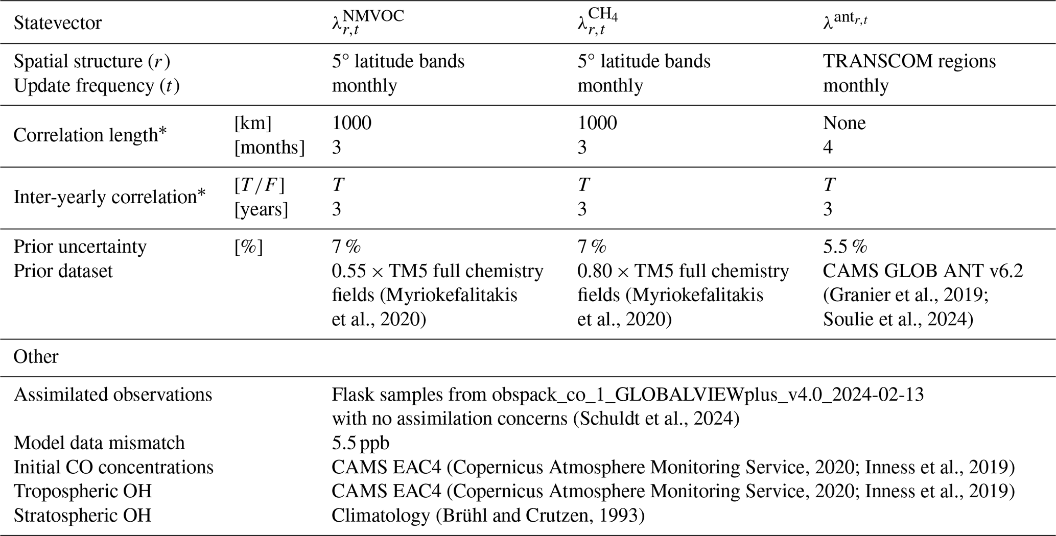
^* This represents the correlation distance or time after which the correlation strength decays by a factor of e.

A benefit of the long-window step is that we optimise several years at once, which allows the system to find robust, repeating inter-annual patterns in the flux updates. In turn, this minimises the risk of aliasing such slowly varying (annual and seasonal) background changes in the short-window inversion. Another practical benefit of the long-window is its computational efficiency, as we can initialise a range of short-window optimisations in parallel from a single long-window solution in parallel. For details on the design philosophy of the long-window/short-window inversion framework, as well as a demonstration of the system for CO₂, we refer to van der Woude (2024).

Prior chemical CO production fields from NMVOC and CH₄ oxidation for the long-window inversion are taken from a TM5-MP chemistry run with extended hydrocarbon chemistry for 2018, following Myriokefalitakis et al. (2020). In this dataset OH was reported to be too high, which led to overcompensation in the chemical CO production terms. To avoid strongly biased start-conditions, we pre-scaled the NMVOC and CH₄ fields. The pre-scaling factors for secondary CO production from NMVOC and CH₄ oxidation were partly chosen to align our prior global budgets with established top-down estimates (e.g. Hooghiemstra et al., 2012a; Zheng et al., 2019; Naus et al., 2022) and partly informed by visual inspection of prior and posterior CO mole fractions from initial forward runs. Additionally, to represent known inter-annual variability in the CH₄, we scaled the CH₄ oxidation fields to the CH₄ atmospheric growth rate from NOAA (Lan et al., 2022).

Our posterior long-window fluxes (Fig. A1) and corresponding CO mole fraction residuals are within established literature values. Because these background fields behave as expected – and we already evaluate the background residuals most relevant to our 2019 case study in Fig. 2 we do not elaborate on it further here.

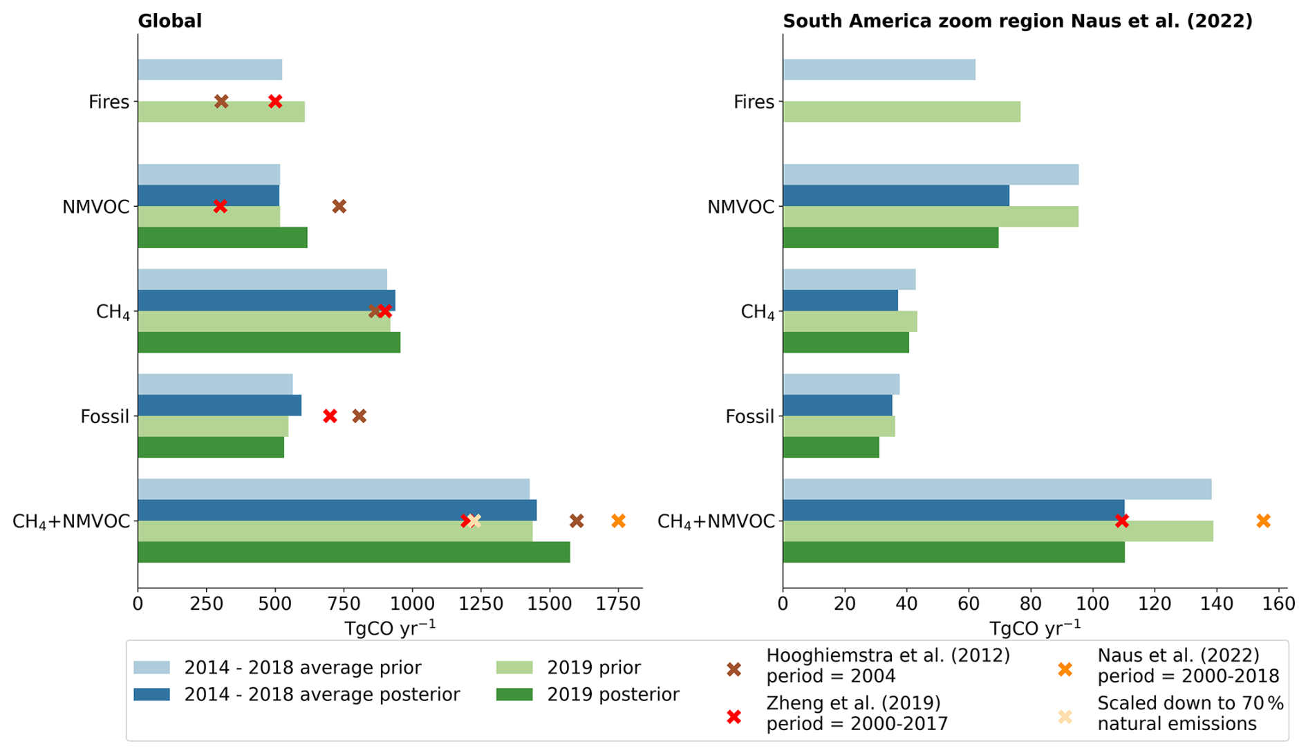
Figure A1 Long-window inversion CO budget overview. Note that the zoom region in Naus et al. (2022) spans from 75 to 39° W and from 28° S to 8° N.

A2 Data selection and scaling factor transformation

We applied a condition (observed X_CO >= 125 ppb | simulated (cycle prior) X_CO >= 125 ppb) for selecting X_CO to assimilate and a scaling factor transformation to avoid negative posterior emissions. By including the “or simulated X_CO” criteria, we make sure that the inversion has freedom to scale down a fire when it is modelled in the short-window prior but not observed.

In Table A2, as well as the independent MOPITT X_CO < 125 ppb in Table A2, provide evidence that these decisions did not or not strongly degrade the simulated columns for the lowest bin. It shows that the simulated “background” retrievals did not result in systematically overestimated “background” columns.

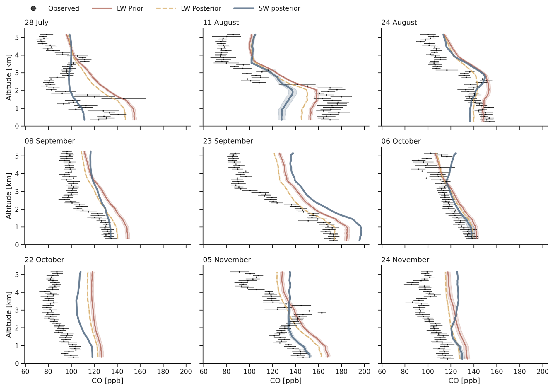
Figure A2 Comparison of measured and simulated carbon monoxide (CO) vertical profiles from nine research aircraft flights near Manaus (2.595° S, 60.209° W), each containing approximately 50 individual measurements (total = 455). Coloured lines show the ensemble mean of the simulated profiles (150 ensemble members for both inversions), and shaded regions indicate the ensemble standard deviation. The short-window posterior results are derived from the GFED5.1_TROPOMI inversion. Black points represent observed profiles with each point representing a time interval average (median length of 42 s and 42 samples per interval); error bars denote the corresponding standard deviation.

Table A2 Mean absolute error (or residual) and the standard deviation of the residuals per observed X_CO bin. Extension of Table 3 with the subset of TROPOMI X_CO that was rejected for assimilation by the (observed X_CO > 125 ppb | simulated (cycle prior) X_CO > 125 ppb) criteria.

A3 Comparison against vertical profiles near Manaus

The TM5 simulations reproduce the observed vertical CO profiles over Manaus reasonably well (Fig. A2). Across the nine flights, the short-window posterior yields a mean absolute percentage error of 19 %, consistent with the the ATTO tower evaluation (Fig. 3). In the lower troposphere, the short-window posterior (blue) generally aligns more closely with the observations than the long-window posterior (orange). This improvement is driven primarily by the higher transport resolution (6° × 4° versus 1° × 1°) and, to a lesser extent, by sensitivity to fire emissions within 3 d of the profile measurements.

In a few cases (28 July, 11 August, and 5 November), we detect limited (lower-)profile sensitivity to prior fire emissions in the short-window inversion (not shown). For these dates, the differences between the long- and short-window posteriors in the lower half of the profiles are consistent with reductions in upwind tropical forest fire emissions around that period (see, e.g., Fig. 5). However, because the aircraft did not sample intense, freshly lofted smoke plumes, this comparison remains inconclusive for evaluating short-window performance. To fairly evaluate the short-window performance, targeted in-plume measurements would be critical.

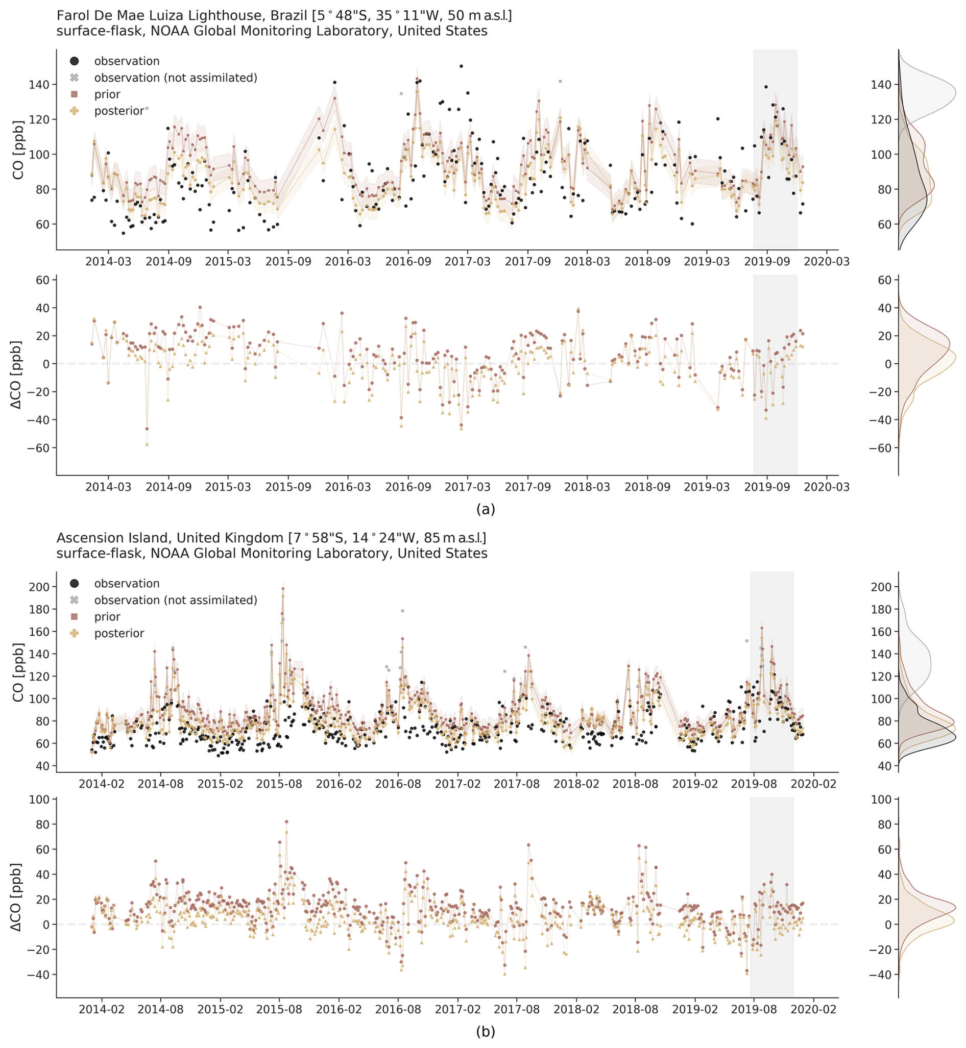
Figure A3 Comparison of observed (black/gray) and simulated CO mole fractions at ASC and NAT from the long-window inversion. Prior simulations are shown in red and posterior simulations in yellow. Shaded areas represent one standard deviation away from the ensemble mean together with the model–data mismatch. Top panels show CO mole fractions, bottom panels show residuals (model – observation), both with corresponding distributions on the right. The grey shaded box indicates the short-window simulation period.

Figure A2 also demonstrates that even when observed profiles suggest substantial fire contributions (e.g. 11 August), an improved model–observation match is not guaranteed. We attribute this partly to the spatial error correlations imposed in the inversion, which distribute emission adjustments across a broader upwind region rather than allowing independent changes at the grid-cell level. Additionally, emissions are optimised over 3 d windows rather than daily, limiting the system’s ability to capture highly localised plume peaks. These results only underscore a fundamental characteristic, namely that atmospheric inversions such as ours are not designed to constrain super-local, day-specific plumes.

The Manaus profile comparison show that the long-window inversion exerts only a minor influence on CO levels over the Amazon (typically < 10 ppb). Because we did not assimilate local flask observations, the long-window inversion is effectively insensitive to the sub-regional variability captured in the lower half of the aircraft profiles. In addition, the current long-window configuration was intentionally configured to adjust only large-scale, slowly varying components of the global CO budget which restricts the inversion's freedom to constrain such local fluxes in central Amazonia. As a result of these choices, we find the long-window prior ensemble spread is narrow and the posterior remains close to the prior in the Manaus profiles.

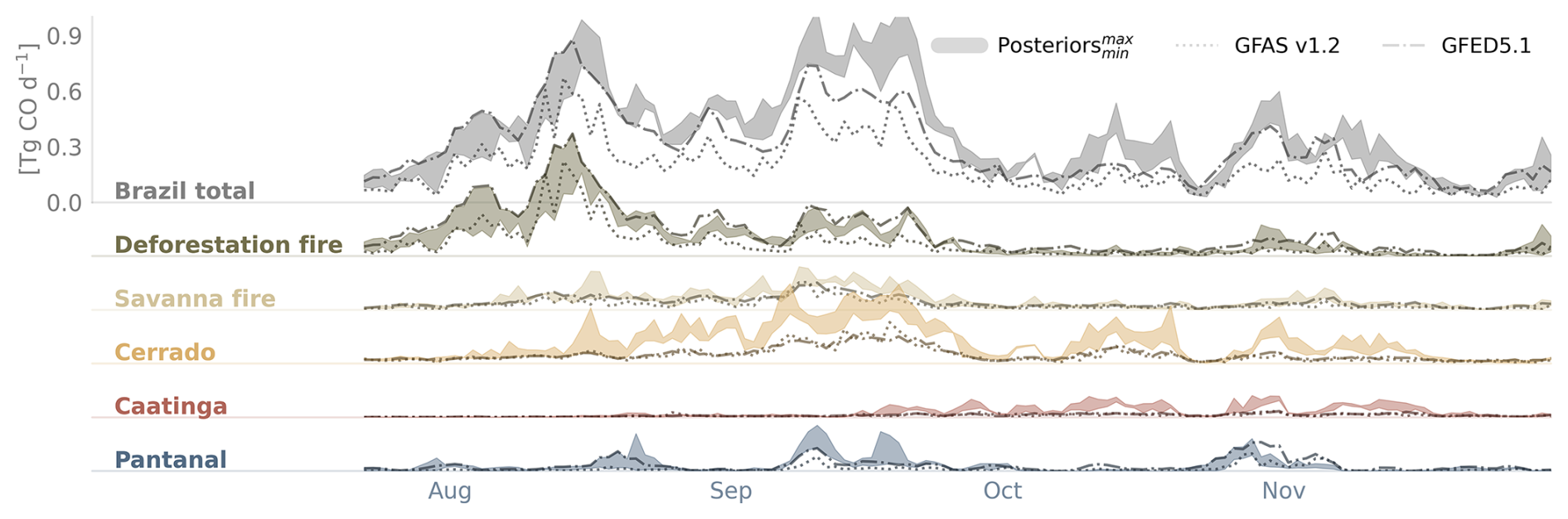
Figure A4 Same as Fig. 5 in the main text, but with the shaded area showing the full posterior range (minimum to maximum) instead of the posterior mean.

A persistent positive residual that averages around 20 ppb remains in the free troposphere of the simulated profiles. The bias reflects, at least in part, large-scale transport or flux errors. This is demonstrated by Fig. A3, which shows long-window posterior residuals of similar magnitude at Farol de Mae Luiza (NAT) – and at times also at Ascension Island (ASC) – during July–December 2019. These locations frequently influence free tropospheric air masses near Manaus during this period of the year. Nonetheless, NAT and ASC remain surface sites and may therefore not capture potential unresolved biases in CO fluxes that originate from the African mainland to their full extent. As a consequence, we cannot conclusively determine how much potential large-scale transport or flux errors contribute to the free-tropospheric residuals observed over Manaus.

Alternatively, the residual could reflect local-scale flux errors and/or in vertical mixing/boundary-layer venting. Previous studies have identified TM5 as fast-mixing compared to other chemistry transport models (Krol et al., 2018; Jin et al., 2025; Remaud et al., 2023). The frequent lack of steepness in the simulated profile vertical gradients are indeed indicative of too much (deep convective) vertical mixing. However, we consider major vertical mixing biases for our full domain and study period unlikely for two reasons: (1) excessive upward mixing would also require low CO in the boundary layer – especially in the unoptimised long-window prior – which is not (systematically) evident from the Manaus profile comparison; and (2) substantial vertical mixing errors would be expected to produce inconsistent short-window results between the MOPITT and TROPOMI driven inversions, given their different averaging-kernel structures. Instead, we find highly consistent solutions. Although this does not necessarily confirm that TM5 does not have any vertical-mixing issues, it does demonstrate that it unlikely presents itself as dominant driver of the free-tropospheric residual.

We estimated the sensitivity of our reported emission estimates to a potential 20 ppb systematic free tropospheric bias that could be propagated through the X_CO we assimilate. We found that such a bias would limit changes in fire emissions to approximately 10 % for both instruments when we conservatively assume the bias to persist across the entire domain to the tropopause throughout the simulation period. This potential underestimate of 10 % (4.7 out of ∼ 47 TgCO in the Brazilian fire emissions) remains well within the reported 15 TgCO structural uncertainty and would not alter our conclusions.

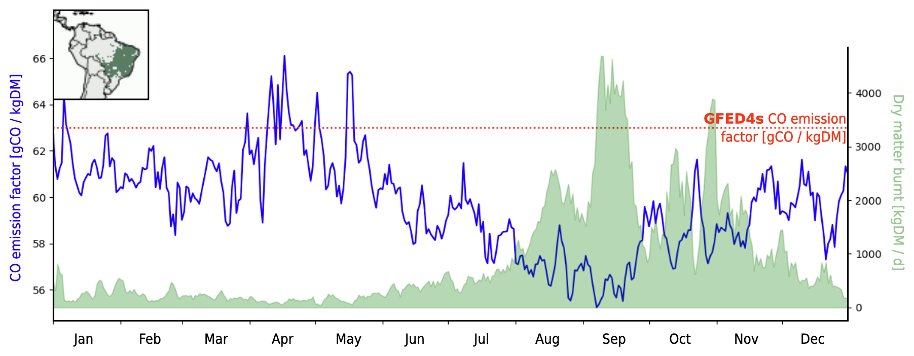
Figure A5 Seasonality of the savanna CO emission factors (EF; blue; left axis) averaged over the region indicated in the inset panel from GFED5.1 (the EFs are weighted by dry matter). The green shaded area shows the region total kg dry matter (DM; right axis). The red line indicated the fixed emission factor that was previously used in GFED 4.

A4 Posterior spread in fire emissions

The posterior spread is generally is small and tends to fall outside the prior-range for Cerrado, Caatinga and Amazon-biome-savanna fires. The only notable exception is early on in the season for deforestation fires. While the TROPOMI inversions there tend to scale towards the GFAS v1.2 emissions, the GFED5.1_MOPITT inversions lacks constraints due to the 1-month instrument outage (Sect. 2.5.1). This presumably is resulting in the large posterior spread, while later on in September with active MOPITT constraints the posterior spread reduced rapidly even though the prior spread was very large there.

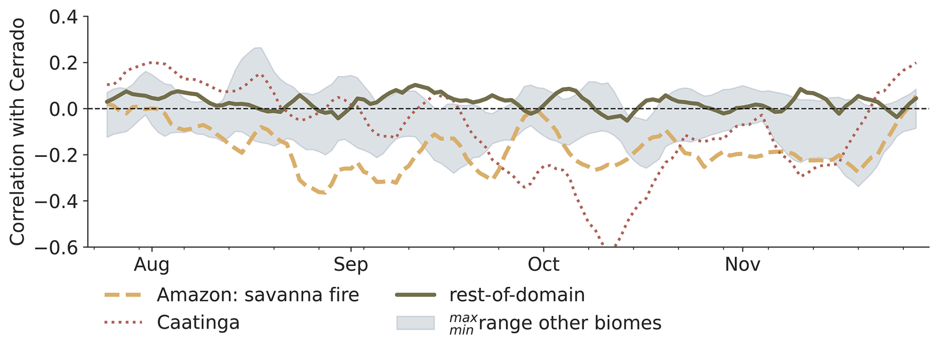
Figure A6 Six-day rolling average correlation between the ensemble of posterior Cerrado emissions and the ensemble of posterior emissions from other biomes (definitions as indicated in Fig. 4). The shaded region represents the minimum-maximum range of correlations across other biomes/fire types in Brazil (incl. Amazon: other dominant fire type, Amazon: deforestation fire, Pantanal, Atlantic forest). Based on the GFED5.1_TROPOMI inversion.

A5 Emission factors

Figure A5 illustrates the general behaviour of CO emission factors (EFs) for savanna fires in the Cerrado/Caatinga savannas, as represented in GFED5.1. The figure shows that the daily, dry-matter-weighted CO EF (blue line) is dynamic, fluctuating throughout the year. Early in the season, during more humid conditions, the EFs are higher. During the peak fire season (August-October), when fuels are dry, the vast majority of dry matter is combusted (green area) and average EF decreases to approximately 55–58 g CO kg DM⁻¹. This is substantially lower than the static EF of 63 g CO kg DM⁻¹ used in the previous GFED 4 inventory (red line). Later in the season the EF increases again; Vernooij et al. (2023) hypothesise that this reflects an increased contribution from woody fuels that become dry enough to burn.

A6 Correlation with Cerrado emissions

Figure A6 shows the six-day rolling average correlation between the posterior Cerrado emissions and those of other biomes. Overall, the Cerrado emissions show very weak correlations with adjacent regions. This indicates that the TROPOMI and MOPITT data provide sufficient observational constraints to disentangle distinct regional emission signals. This implies that the emission adjustments in the Cerrado do not merely act as a spatial compensation mechanism for surrounding structural biases.

We note two brief exceptions to this weak correlation. First, a strong positive correlation with the Caatinga occurs in mid-October. This coincides with a shift from the typical south-east trade winds to more easterly winds, which likely causes Caatinga air masses to mix with the Cerrado to an extent that limits the inversion's ability to perfectly separate the signals. Second, we observe occasional anti-correlations with savanna-type fires within the Amazon biome. This is actually an encouraging feature of the inversion: while our prior covariance matrix structurally links these fires to the rest of the Amazon biome, the assimilated observations provide independent sufficient information to break this prior assumption, dynamically linking their behaviour to the Cerrado fires instead.

A7 Carbon emissions per biome

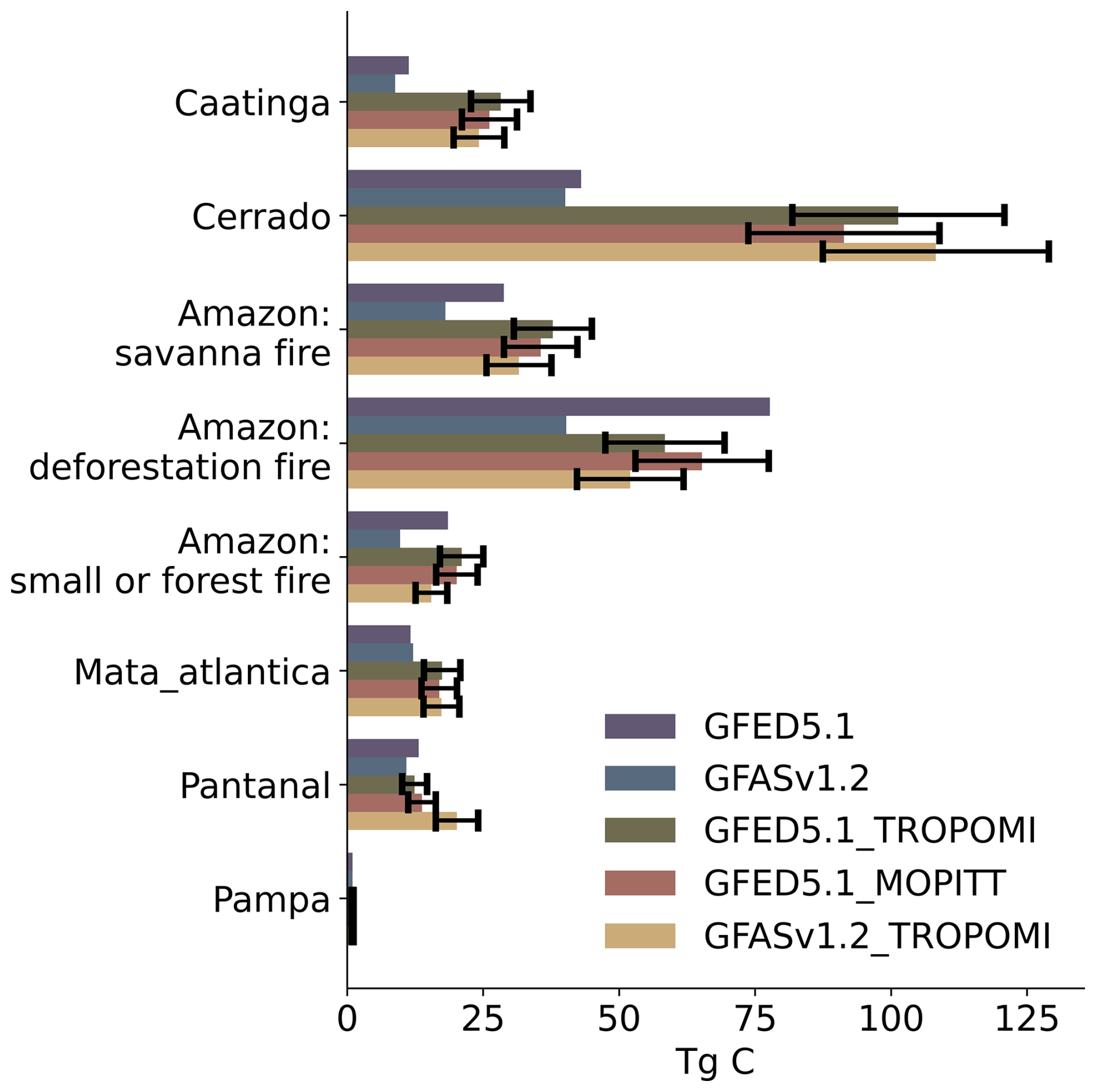
Figure A7 Carbon emissions (C from CO and CO₂) per biome. Posterior carbon emissions were inferred from CO using the prior inventory's $\frac{{\mathrm{CO}}_{\mathrm{2}}}{\mathrm{CO}}$ emission factor ratios at the location/time of the emission. The error bars represent the min/max range for a hypothetical 20 % error margin on the ${\mathrm{CO}}_{\mathrm{2}}/\mathrm{CO}$ emission factor ratios.