The dynamics and atmospheric impact of fire-induced circulations in idealised large-eddy simulations inspired by the Santa Coloma de Queralt fire

We studied the factors governing the existence of fire-induced circulations ahead of the flaming zone and the impact of these circulations on the thermodynamic structure of the atmospheric boundary layer. To study the circulation, we used MicroHH to create a high-resolution (25 m) turbulence-resolving 3D large-eddy simulations (25.6 km×38.4 km) of a stationary fire under realistic atmospheric conditions. The setup was inspired by field observations of fire characteristics and a radiosonde from the Santa Coloma de Queralt fire (Catalonia, Spain, 24 July 2021). The stationary fire enabled us to isolate the persistent impacts of the fire on the atmosphere.

Our results indicate that the existence of a fire-induced circulation is governed by the wind speed component aligned with the circulation. In our simulations, the circulation consisted of updrafts above the fire, downdrafts 2 km ahead, and reversed surface winds between the updrafts and downdrafts. With higher wind speeds in the direction of the circulation, the reversal of the surface winds decreases. Consequently, the circulation dissipates, since the reversed winds connect the updrafts and downdrafts into a circulation. Hence, explaining why fire-induced circulations are not always present.

The thermodynamic impact of the circulation is driven by the updrafts and downdrafts, causing 2 km of deepening, followed by 2 km of thinning of the atmospheric boundary layer ahead of the fire. Future research with non-stationary fires is required to quantify the impact of the modified thermodynamics and wind patterns on fire behaviour.

1 Introduction

Extreme wildfire events are defined by fire behaviour that surpasses the extinguishing capacity of fire services, indicated by factors such as high rates of spread, erratic spotting, or fireline intensities exceeding 10 MW m⁻¹ (Tedim et al., 2018). During events with such intensity, the high fireline intensity can trigger significant upward convective motions (i.e. pyro-convection), which affect the wind speed and direction in the direct surroundings of the wildfire. The altered winds will change the fire behaviour (Sun et al., 2009), impacting the fireline intensity and, subsequently, feed back on the pyro-convection. Recent extreme wildfire events in Spain (2021) and Portugal (2017) that triggered pyro-convection spread significantly faster than predicted (Commissão Téchnica Independente, 2017; Castellnou et al., 2022), with some unexpectedly continuing to burn throughout the night despite worsening burning conditions.

Part of this unexpected fire behaviour can be explained by the modification of the surface winds by convective fires. Specifically, the acceleration of the rear inflow by convective fires (Potter, 2012) offers an explanation for the faster-than-predicted fire spread (Castellnou et al., 2022), as current operational fire spread models do not account for the effects of fire-modified winds (Kochanski et al., 2013). The other part, the continued nighttime burning, has recently been attributed to the global increase in nighttime temperatures due to climate change (Balch et al., 2022). However, we hypothesise that, in addition to the global climate trend in nighttime temperature, extreme wildfire events can locally modify atmospheric surface temperature and humidity downwind, thereby enhancing the local atmospheric conditions for nighttime fire activity.

Recent work by van der Aa et al. (2026) shows that fires can trigger the formation of rotor-like circulations ahead of the flaming zone, here further referred to as fire-induced circulations. These circulations are also visible in the Doppler measurements of Banta et al. (1992), consisting of the convection inside the plume, downwind downdrafts and reversed surface winds. At night, the downdrafts of this circulation will transport relatively warm, dry air towards the surface, thereby counteracting nighttime cooling and moistening. Hence, through downdrafts in the circulation, extreme wildfire events could enhance atmospheric surface conditions for nighttime fire activity. Simultaneously, we recognise that not all previous simulations (e.g. Filippi et al., 2018) show reversed surface winds, suggesting that the development of a fire-induced circulation depends on specific atmospheric conditions.

Both van der Aa et al. (2026) and Banta et al. (1992) only show the kinematic structure of the fire-induced circulation. Hence, the impact of the circulations on the thermodynamic structure of the atmosphere remains unexplored. However, the simulations by van der Aa et al. (2026) provide a first clue into the drivers behind the fire-induced circulation. A comparison between their simulations suggests that increasing background wind shear strengthens the circulation. Therefore, we hypothesise that directional wind shear is essential for the development of fire-induced circulations. Simultaneously, we acknowledge that for situations with pyrocloud formation, pyrocloud-induced precipitation can also cause fire-induced circulations (Wang et al., 2025). However, as we elaborate below, we will focus on fire-induced circulations during dry pyro-convection. Hence, precipitation is not considered in this study.

To investigate the factors governing the fire-induced circulations and their impact on the atmosphere, we will use a LES setup with a stationary fire similar to Badlan et al. (2021a, b). Keeping the fire stationary eliminates the complex coupled fire-atmosphere feedbacks, allowing us to isolate and quantify how the fire alters its surrounding atmosphere. However, contrary to Badlan et al. (2021a, b), who used a fully synthetic setup, we based our simulations on observations from a real extreme wildfire event, ensuring realistic meteorological conditions and a realistic size and intensity of the stationary fire.

Similar to van der Aa et al. (2026), we used observations and measurements from the first day of the Santa Coloma de Queralt (SCQ) fire, which took place on 24 July 2021, in Catalonia, Spain (CFRS, 2022; Castellnou et al., 2022). The SCQ fire is a relatively well-documented extreme wildfire event with measurements of both the fire characteristics and the atmosphere, which is rare given the dangerous measurement conditions during such events (Werth et al., 2016; Moisseeva and Stull, 2021). Moreover, the SCQ fire also offers a scientifically interesting scenario. In short, it is one of the extreme wildfire events observed to continue burning throughout the night, maintaining a dry convective plume until midnight (Ribau et al., 2022). Furthermore, firefighter observations report the presence of reversed surface winds ahead of the fire, indicating a fire-induced circulation. In line with these observations, simulations by van der Aa et al. (2026) showed a fire-induced circulation for the first day of the SCQ fire. Hence, the SCQ provides the right conditions for our simulations to investigate which factors govern the fire-induced circulation and their impact on the thermodynamic structure of the atmosphere.

For the LES, we used MicroHH (van Heerwaarden et al., 2017), a proven turbulence-resolving LES tool for simulating convective and pollution plumes (van Heerwaarden et al., 2014; Ražnjević et al., 2022). Furthermore, MicroHH allows for a landscape-scale domain (order of 10 km) while supporting a high resolution (order of 10 m). Hence, with MicroHH, we can simulate the large-scale ambient turbulent structures that define the atmospheric boundary layer while resolving the small-scale turbulent structures within the fire-induced plume and the downwind circulation.

Using the MicroHH LES setup inspired by the SCQ fire, we focus on two objectives in this study. The first objective is to quantify the impact of a fire-induced circulation on the thermodynamic structure of the atmosphere. Subsequently, our second objective is to determine what atmospheric factors govern the development of a fire-induced circulation.

2 Methods

To achieve our objectives, we designed four LES experiments using MicroHH inspired on the SCQ fire. Section 2.1 describes the available observations of the SCQ fire that we use to set up our LESs and to evaluate how well the simulation captures the observed meteorological conditions. Next, we present the core simulation setup of MicroHH in Sect. 2.2 informed by the observations of the SCQ fire, which subsequently serves as the foundation for all four LES experiments described in Sect. 2.3.

2.1 Santa Coloma de Queralt fire

The SCQ fire started on 24 July 2021 at 14:00 UTC (LT−2) in Catalonia, Spain, with the ignition point located at 41.52329° N, 1.369071° E. It spread eastward under a predominantly westerly wind and directly developed a convective plume (Fig. 1a). Occasional overshooting created short-lived pyrocumulus clouds between 17:00–19:00 UTC, termed overshooting pyrocumulus (oPyroCu) by Castellnou et al. (2022). After 19:00 UTC, no further pyrocloud formation was observed (CFRS, 2022). The change from moist convection (i.e. pyrocloud formation) to dry convection (i.e. no pyrocloud formation) coincided with the arrival of the sea breeze at 19:00 UTC and sunset (19:41 UTC). The sea breeze caused the advection of moisture combined with backing of the wind from 300 to 240–270° (Fig. 1d). The moisture advected by the sea breeze, combined with the cooling around sunset, caused an increase in relative humidity (Fig. 1c). Nevertheless, observations indicate that the moistening did not result in renewed pyrocloud formation (Fig. 1a). Simultaneously, despite the cooling and moistening of the atmosphere around sunset (Fig. 1c), the SCQ fire maintained a dry convective plume until midnight (22:00 UTC).

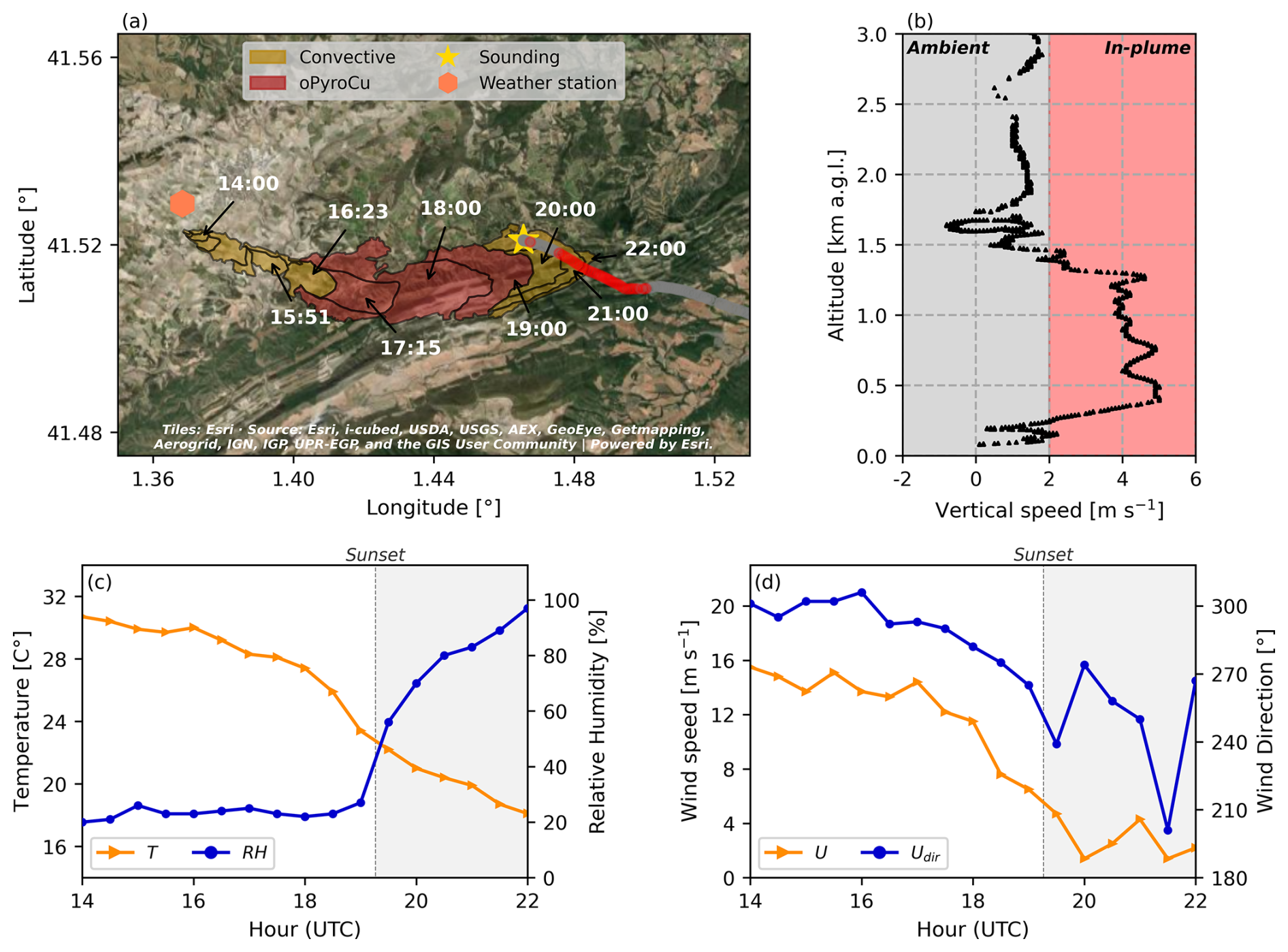
Figure 1 (a) The fire spread during the first day of the SCQ fire in UTC (LT−2), including the locations of the sounding (star) and the synoptic weather station (hexagon). Additionally, the grey and red circles show the horizontal displacement of the radiosonde during its ascent. The red circles highlight the part of the ascent with rising speeds above 2 m s⁻¹, which indicates that at these locations the radiosonde was measuring within the convective core of the plume, since in ambient conditions, the maximum rising speed of a radiosonde is 2 m s⁻¹ (Castellnou et al., 2022). (b) The rising speed of the radiosonde during its ascent vs. the altitude a.g.l., with the grey and red shade indicating whether the radiosonde was out- or inside the convective plume based on the 2 m s⁻¹ threshold. (c) The evolution of the temperature (T) and relative humidity (RH) during the SCQ fire measured by the synoptic weather station. (d) The same as (c) but for the 10 m wind speed (U) and direction (U_dir). The sounding and synoptic observations are part of a larger observational dataset described by Castellnou et al. (2022). The fire perimeter map is an updated version of the map provided by Castellnou et al. (2022), incorporating recent insights into the fire spread behaviour of the SCQ fire.

At 19:51 UTC, a radiosonde was released at the right flank of the fire (yellow star; Fig. 1a) into the convective plume of the SCQ fire that measured vertical profiles of temperature, specific humidity, wind speed and rising speed. A description of the equipment and measurement techniques is provided by Castellnou et al. (2022). The radiosonde drifted predominantly eastward during its ascent (grey and red circles; Fig. 1a), with measurements starting at 80 m a.g.l. (above ground level; Fig. 1b). In ambient conditions, the maximum rising speed of a radiosonde is ±2 m s⁻¹. Rising speeds above 2 m s⁻¹ indicate a vertical acceleration of the radiosonde by the convective motions of the wildfire plume (Castellnou et al., 2022). Hence, from the rising speed during the ascent of the radiosonde (Fig. 1b), we conclude that the radiosonde measured inside the convective plume of the SCQ fire between 0.3–1.5 km altitude a.g.l. In addition to measurements within the convective plume, the radiosonde recorded a partial profile of the ambient temperature and relative humidity during its descent.

Consequently, we will use the radiosonde measurements to evaluate how well the simulated pyro-convection and the ambient conditions compare to reality. For the evaluation, we will focus on comparing the observed and simulated temperature profiles. Furthermore, we will also compare the measured wind speed in the convective plume with the simulated wind speed. The measured wind speed during the descent of the radiosonde in the surroundings of the plume and the measured specific humidity are not used for the comparison. We consider the wind speed measurements during descent unreliable due to the high descent speed of the radiosonde (8–9 m s⁻¹). The specific humidity measurements, on the other hand, are reliable but redundant for evaluating our simulation, as both observations and the simulation indicate a dry convective plume (i.e. no pyro-clouds). Hence, the simulation was sufficiently dry.

The radiosonde measurements were taken using the Windsonde S1H2 system, which has a sensor accuracy for temperature and pressure of 0.3 °C and 1.0 hPa (SparvEmbedded, 2016). Comparison of the S1H2 sondes to regular meteorological Vaisala RS41-SG sondes has shown two challenges with their measurements. Firstly, the S1H2 sonde shows a slow humidity response at cloud tops (Castellnou Ribau et al., 2025). Secondly, the S1H2 sondes measure relatively noisy wind profiles in turbulent conditions (Bessardon et al., 2019). The first concern is irrelevant to our study as we focus on a dry convective plume. The second challenge results indeed in a relatively noisy wind pattern inside the atmospheric boundary layer (see Fig. 6c, Sect. 3.1). Nonetheless, it is sufficient to provide a range of realistic wind speeds observed inside the atmospheric boundary layer. Furthermore, despite the noisy signal, it provides a clearly distinguishable signal of the capping inversion. Moreover, an exact match of the radiosonde measurements with an LES simulation is always impossible inside an atmospheric boundary layer, as radiosondes provide instantaneous measurements of the turbulence, whereas LES focuses on producing similar turbulence on average. Hence, the goal of the comparison is not a point-by-point match, but rather an evaluation of how well our LES setup reproduces the overall characteristic of the observed plume and atmospheric boundary layer structure in terms of mixed layer potential temperature, wind speed and boundary layer height.

2.2 Core simulation setup

As discussed in the introduction, we aim to isolate the effect of the fires on the atmosphere, specifically focusing on the fire-induced circulation during dry pyro-convection. Hence, in our MicroHH simulation setup (van Heerwaarden et al., 2017), we prioritise atmospheric realism while significantly simplifying the simulated fire behaviour to isolate the fire's impact on the atmosphere.

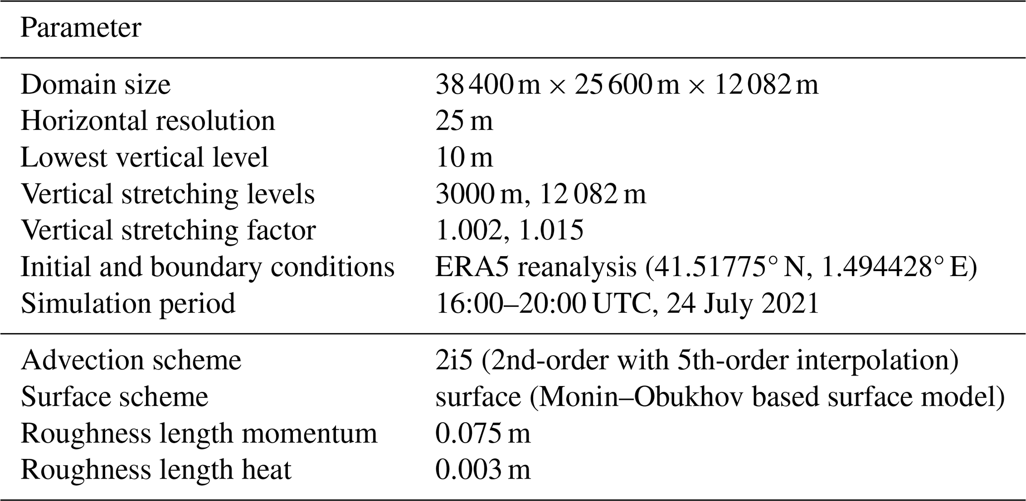
MicroHH is configured with a domain of $\mathrm{38.4}\mathrm{km}\times \mathrm{25.64}\mathrm{km}\times \mathrm{12}\mathrm{km}$ ($x\times y\times z$). The domain is elongated eastward (i.e. in the positive x direction) as the observed plume from the SCQ fire developed eastward, and MicroHH uses periodic boundaries. To prevent the unwanted recirculation of the simulated plume over the eastern border, we found that a domain of 38.4 km in the eastward direction was sufficiently large (see Appendix A). The simulations use an equidistant horizontal resolution of 25 m and a stretched vertical grid starting at 10 m above the surface (Table 1).

Table 1 An overview of the main simulation parameters of MicroHH (van Heerwaarden et al., 2017). The full simulation setup to reproduce this study is provided in the associated data repository (Roelofs et al., 2025).

Each simulation covers a 4-h period (16:00–20:00 UTC) on 24 July 2021. For the analysis (Sect. 3), we used the last hour of the simulations (19:00–20:00 UTC) as it matches the timing of the sounding (19:51 UTC) and the period during which local firefighters reported the reversal of the surface winds. Hence, this is the period in which we expect a fire-induced circulation to develop. The first two hours serve as spin-up time, after which the fire is initialised. This provides an additional hour of spin-up time (18:00–19:00 UTC) to allow the convective plume to develop, ensuring a dry convective plume between 19:00–20:00 UTC.

Detailed implementations of the fire and meteorological boundary conditions are described in Sects. 2.2.1 and 2.2.2, respectively.

2.2.1 Fire implementation

To implement a fire in MicroHH, we added a stationary moon-shaped area with a constant heat flux of 145 kW m⁻² (Fig. 2) between 18:00–20:00 UTC on top of the ambient surface fluxes from ERA5 (see Sect. 2.2.2). To prevent numerical errors, we applied Gaussian smoothing (σ=25 m) to smooth the transition from the ambient surface fluxes (∼1–10² W m⁻²) to the fire fluxes (∼10⁵ W m⁻²). The stationarity is justified by the significantly smaller rate of spread of the fire compared to the wind speed, which makes the movement of the fire negligible from an atmospheric perspective, the main focus of our study. The significant advantage of stationarity is that it enables temporal averaging of the plume to detect persistent patterns in the impact of the fire on the atmosphere. Additionally, stationarity eliminates the need for fuel and topographic maps. Hence, the surface of the simulated domain is flat and homogeneous. Although the local topography is simplified to a flat plain, the average elevation is accounted for through the ERA5 pressure field (see Sect. 2.2.2).

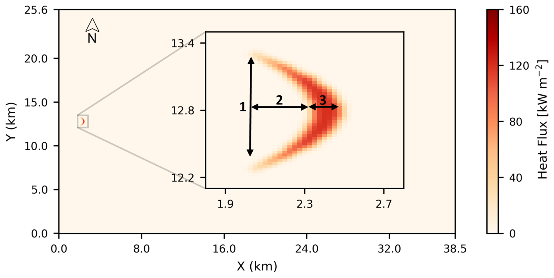
Figure 2 The surface heat flux in the simulation, including Gaussian smoothing (σ=25 m), with a zoom-in on the moon-shaped implementation of the fire. The arrows indicate the dimensions of the implemented wildfire, which are 1100 m (1), 350 m (2), and 150 m (3).

The moon-shaped area is based on observations of the SCQ fire by the Catalan Fire Service, including the fire perimeters shown in Fig. 1a, which indicate a fire 1100 m wide and 350 m deep, with a 150 m deep flaming zone at the head of the fire (arrows 1, 2, and 3 in Fig. 2). To implement it, we define the shape based on two quadratic equations, Eqs. (1) and (2), which represent the east and west borders of the flaming zone, respectively:

$$\begin{array}{}\text{(1)}& {\displaystyle }& {\displaystyle }{x}_{\text{east}}\left(y\right)=x_{\mathrm{0}}+L_{\text{east}}\left[\mathrm{1}-{\left({\displaystyle \frac{(y-y_c)}{\frac{W}{\mathrm{2}}}}\right)}^{\mathrm{2}}\right]\text{(2)}& {\displaystyle }& {\displaystyle }{x}_{\text{west}}\left(y\right)=x_{\mathrm{0}}+L_{\text{west}}\left[\mathrm{1}-{\left({\displaystyle \frac{(y-y_c)}{\frac{W}{\mathrm{2}}}}\right)}^{\mathrm{2}}\right]\end{array}$$

with x₀ representing the distance of the fire to the west border of the domain (2000 m), y_c representing the centre of the fire on the y axis (12 812.5 m) and W the width of the fire (arrow 1 in Fig. 2; 1100 m). Lastly, L represents the distance between x₀ and the peak of the parabole at y_c, so for the west border (L_west) of the flaming zone (Eq. 2) it represents arrow 2 in Fig. 2 (350 m), while for the east border (L_east) it represents arrows 2 + 3 (500 m).

The flaming zone is defined as the area between Eqs. (1) and (2) where $x_{\text{west}}\le x\le x_{\text{east}}$. At the flanks of the fire where $y-y_c=\pm \frac{w}{\mathrm{2}}$, the dimensionless ratio ${\left(\frac{(y-y_c)}{\frac{W}{\mathrm{2}}}\right)}^{\mathrm{2}}=\mathrm{1}$. Hence, x_west=x_east at the flanks, therefore resulting in the end of the flaming zone. When moving from the flanks to the centre of the fire (y=y_c), the dimensionless ratio goes to 0, resulting in the maximum difference between Eqs. (1) and (2), which equals $L_{\text{east}}-L_{\text{west}}=\mathrm{150}$ m, the maximum flaming zone depth (arrow 3 in Fig. 2).

Furthermore, the constant heat flux means that we do not explicitly simulate the combustion. Instead, we derived the fire line intensity (FLI in kW m⁻¹) based on Byram's definition of the fire line intensity (Byram, 1959):

$$\begin{array}{}\text{(3)}& {\displaystyle }{\displaystyle }\text{FLI}=\mathrm{0.5}H\left[w\left(\mathrm{1.0308}-\mathrm{0.048}\text{FFMC}\right)\right]\text{ROS}\end{array}$$

where ROS represents the observed rate of spread m s⁻¹ determined from the observed fire perimeter (Fig. 1a) using the methodology described by Duane et al. (2024), H the heat content of the fuel in J kg⁻¹ and w the amount of available fuel in kg m⁻². For H, we used an effective heat content of 14 700 kJ kg⁻¹, which is within the average reported H for experiments (Finney et al., 2021). Furthermore, we added two correction factors. Firstly, following Rio et al. (2010), we applied a correction factor of 0.5 based on the assumption that 50 % of the radiative heat is lost to the surrounding atmosphere, meaning that only 50 % of the FLI contributes to the buoyant plume formation. Secondly, similarly to Lareau and Clements (2016), we correct the available fuel based on the fine fuel moisture content, FFMC (Nelson, 2000), albeit with a different approach. The FFMC correction factor in Eq. (3), 1.0308−0.048FFMC, is designed under the assumption that all fuel is available for burning at a relative humidity of 3 %, and that the amount of available fuel decreases linearly with increasing relative humidity until the extinction relative humidity of 21 % is reached.

For the SCQ fire (between 19:00–20:00 UTC), the ROS is determined at 1 m s⁻¹, and w was approximated at 3.3 kg m⁻² based on the dominant fuel type, the pinus halepensis. Furthermore, we estimated the FFMC to be between 0 %–6 % based on the weather station data (Fig. 1). Using Eq. (3), this results in an FLI ranging from 18×10³ to 25×10³ kW m⁻¹. To convert the FLI into a surface flux, we divided the FLI by the flaming zone depth (150 m, arrow 3 in Fig. 2), which resulted in a fire heat flux ranging between 120–170 kW m⁻². Within this range, we selected the mean heat flux of 145 kW m⁻² for the fire in our simulations (see Sect. 2.3).

Lastly, we do not simulate the chemical composition of the fire-induced plume. Instead, we use an inert tracer to represent the plume shape. Consequently, we do not simulate the interaction of the smoke plume with radiation, so shadowing effects are not included. The lack of shadowing effects is expected to have a negligible impact on the outcomes of this study as we focus on the period between 19:00–20:00 UTC, which is around sunset (19:41 UTC). At sunset, the incoming radiation makes a minimal contribution to the energy balance, rendering the shadowing effect negligible.

2.2.2 Meteorological boundary conditions

To create as realistic meteorological conditions as possible in MicroHH, we used the ERA5 reanalysis data (Hersbach et al., 2020) as boundary conditions. ERA5 is considered one of the best currently available reanalysis datasets for studying convective environments (Taszarek et al., 2021). Additionally, the high vertical resolution (28 layers within the lower 2 km of the atmosphere) of ERA5 at hourly intervals captures the pre-fire atmospheric boundary layer, which is the layer where pyro-convection occurs. We retrieved the ERA5 boundary conditions at a single point, the centre of the SCQ fire (latitude: 41.51775°, longitude: 1.494428°), since MicroHH uses periodic boundaries.

Figure 3 shows the ERA5 boundary conditions of the virtual potential temperature (θ_v), specific humidity (q), wind speed (U) and wind direction (U_dir) at 16, 18, and 20:00 UTC. The q and U_dir show moistening of the CBL combined with backing winds, indicating a sea breeze in ERA5 after 16:00 UTC (Fig. 3b and d). Besides moistening, the sea breeze also causes cooling of the boundary layer, which combined with the shift from a positive to a negative surface heat flux between 19:00–20:00 UTC explains the transformation of the convective boundary layer at 16:00 UTC (blue line; Fig. 3a) into a neutral boundary layer ($\mathrm{0}<z<\mathrm{0.5}$ km) capped by a residual layer ($\mathrm{0.5}<z<\mathrm{2}$ km) between 19:00–20:00 UTC (purple dotted line; Fig. 3a), the period of interest for this case study of the SCQ fire. The reduction in turbulence is also visible in the vertical profile of U, which shows the development of a low-level jet at 20:00 UTC (purple dotted line; Fig. 3c).

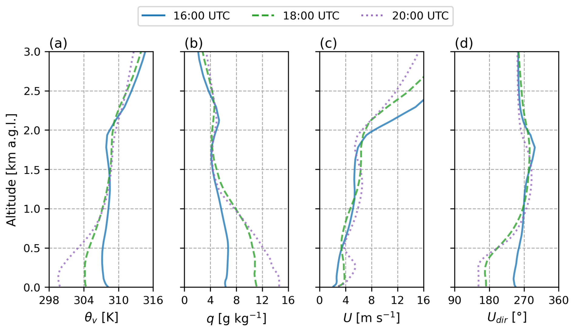
Figure 3 The boundary conditions for MicroHH of θ_v (a), q (b), U (c), and U_dir (d) obtained from the ERA5 reanalysis dataset (Hersbach et al., 2020) using the (LS)²D python package (van Stratum et al., 2023) at 16:00, 18:00, and 20:00 UTC.

The arrival of the sea breeze in ERA5 (after 16:00 UTC) occurs three hours earlier than the observations (see Sect. 2.1). Furthermore, the sea breeze in ERA5 is accompanied by significant backing of the wind (±90°), resulting in southerly winds (Fig. 3d), while the observations indicate only slight backing of the wind by 30–60° (Fig. 1d), which kept the winds predominantly westerly. Previous validation studies of ERA5 in complex terrain show that a horizontal resolution of 31 km is often insufficient to resolve small-scale orographic features, leading to significant discrepancies in local winds (Gualtieri, 2021; Zuo et al., 2025). For the SCQ fire, this suggests that the ERA5 grid is too coarse to resolve the coastal mountain range in Catalonia, which acted as a barrier to the sea breeze, delaying its arrival until 19:00 UTC (CFRS, 2022). Despite the temporal and directional mismatch between the sea breeze in ERA5 and the observations, it does not significantly affect the objectives of our study, since we simulate a stationary fire, meaning the location of the fire inside our simulation is decoupled from the ambient wind direction. This decoupling allows us to focus on understanding the impact of pyro-convection on the atmosphere rather than accurately replicating the observed fire spread under imperfect boundary conditions.

2.3 Experiments

Table 2 lists the four LES simulations using in this study. The first two simulations, ref-run and fire-run, follow exactly the simulation setup described in Sect. 2.2. The only difference is that for the fire-run, a fire is initialised at 18:00 UTC, whereas for the ref-run, no fire is initiated. Consequently, the difference between the fire-run and the ref-run shows the impact of the fire on the atmosphere. Hence, using these two simulations, we can determine the impact of the fire-induced circulation on the thermodynamic structure of the atmosphere, our first objective.

Table 2 Overview of the LES simulations used in this study.

^* Domain extended 25 % eastward (48 km) to avoid recirculation due to the increased zonal wind speed in this sensitivity experiment (Fig. 15).

The last two simulations, fire-run:no-u-advec and fire-run:pg, are modified versions of the fire-run designed to investigate whether the directional wind shear, as hypothesised, governs the development of a fire-induced circulation. In these two simulations, we modified the large-scale forcings of the zonal and meridional wind in two different ways to create increasingly less directional wind shear compared to the fire-run.

In MicroHH, three large-scale forcings are applied to the zonal and meridional wind components (Eqs. 4 and 5, respectivelly): (1) large-scale advection prescribed directly from ERA5 (${\frac{\partial u}{\partial t}}_{\text{lsa}}$ and ${\frac{\partial v}{\partial t}}_{\text{lsa}}$), (2) the pressure gradient implemented through the geostrophic wind (u_g and v_g), and (3) nudging defined by the nudging velocities (u_n and v_n) and a nudging timescale (τ_n) set at 10 800 s.

$$\begin{array}{}\text{(4)}& {\displaystyle }& {{\displaystyle \frac{\partial u}{\partial t}}}_{\text{ls}}\sim \underset{\begin{array}{c}\text{Large scale}\\ \text{advection}\end{array}}{\underbrace{{{\displaystyle \frac{\partial u}{\partial t}}}_{\text{lsa}}}}+\underset{\text{Pressure gradient}}{\underbrace{f_{\mathrm{0}}(v-v_g)}}-\underset{\text{nudging}}{\underbrace{{\displaystyle \frac{u-u_n}{{\mathit{\tau }}_n}}}}\text{(5)}& {\displaystyle }& {{\displaystyle \frac{\partial v}{\partial t}}}_{\text{ls}}\sim \underset{\begin{array}{c}\text{Large scale}\\ \text{advection}\end{array}}{\underbrace{{{\displaystyle \frac{\partial v}{\partial t}}}_{\text{lsa}}}}-\underset{\text{Pressure gradient}}{\underbrace{f_{\mathrm{0}}(u-u_g)}}-\underset{\text{nudging}}{\underbrace{{\displaystyle \frac{v-v_n}{{\mathit{\tau }}_n}}}},\end{array}$$

where f₀ represents the Coriolis parameter of $\mathrm{9.67}\times {\mathrm{10}}^{-\mathrm{5}}{\mathrm{s}}^{-\mathrm{1}}$ based on the center of the SCQ fire (latitude: 41.51775°, longitude: 1.494428°).

Figure 4 shows the large-scale forcing terms for the zonal and meridional wind components based on the fire-sim. Near the surface (<500 m), the large-scale advection term (a) is dominant for the zonal wind component (solid lines), whereas for the meridional wind component (dashed lines), the pressure gradient term (b) is the largest. Hence, to reduce the directional wind shear, we modified the fire-run in two ways: (1) turning off the large-scale advection of zonal momentum after 18:00 UTC (fire-run:no-u-advec) and (2) turning off both large-scale momentum advection and nudging after 18:00 UTC, resulting in a simulation with only a pressure gradient forcing (fire-run:pg). The subsequent changes in vertical wind profiles are discussed in Sect. 3.3.

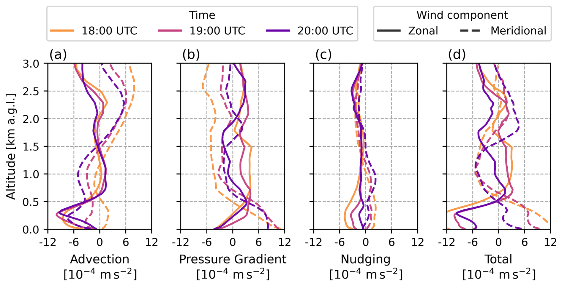
Figure 4 The advection (a), pressure gradient (b), and nudging (c) terms and total change (d) for the zonal (solid lines) and meridional (dashed lines) wind speed over time as presented in Eqs. (4) and (5) in the lowest three km a.g.l. for the fire-run. The vertical profiles represent a line average along the x direction at y=12.8125 km.

3 Results

The analysis is split into three stages. First, we evaluate the extent to which our core simulation setup (Sect. 2.2) compares to the visual observations and sounding measurements (Sect. 3.1). Second, we analyse the atmospheric response to the dry pyro-convection in the fire-run, focusing on the development and subsequent impact of the fire-induced circulation (Sect. 3.2). Lastly, we use the sensitivity experiments (Sect. 2.3) to investigate the impact of the reduced directional wind shear on the development of the fire-induced circulation (Sect. 3.3).

3.1 Comparison with observations

To evaluate the simulated pyro-convection between 19:00–20:00 UTC, we compare the simulated plume shape and vertical profile of the virtual potential temperature (θ_v) and wind speed (U) with visual observations (Fig. 5) and the in-plume radiosonde measurements (Fig. 6). The observed plume of the SCQ fire between 19:00–20:00 UTC is presented in Fig. 5a–c for 19:13, 19:34, and 19:59 UTC. Throughout the hour, a well-developed convection column was observed (1) with occasional overshooting (2) and a horizontally dispersed smoke layer, also called the dispersion layer (3). Here, the distinction between the convection column and the dispersion layer is made visually based on the dominant axis of development: vertical (i.e. convection column) or horizontal (i.e. dispersion layer). The average simulated plume shape between 19:00–20:00 UTC based on the inert tracer is shown in Fig. 5d (grey outline). Similar to the observed plume, the average simulated plume also shows a convection column and a dispersion layer. Occasional overshooting also occurs in the simulation (not shown), but not consistently enough to affect the average plume shape. Additionally, the simulation shows, on average, downward transport of smoke below the dispersion layer, which suggests subsiding motions ahead of the fire front. Although the downward transport of smoke does not become apparent in Fig. 5a–c, it does match descriptions of the plume behaviour provided by local fire fighters.

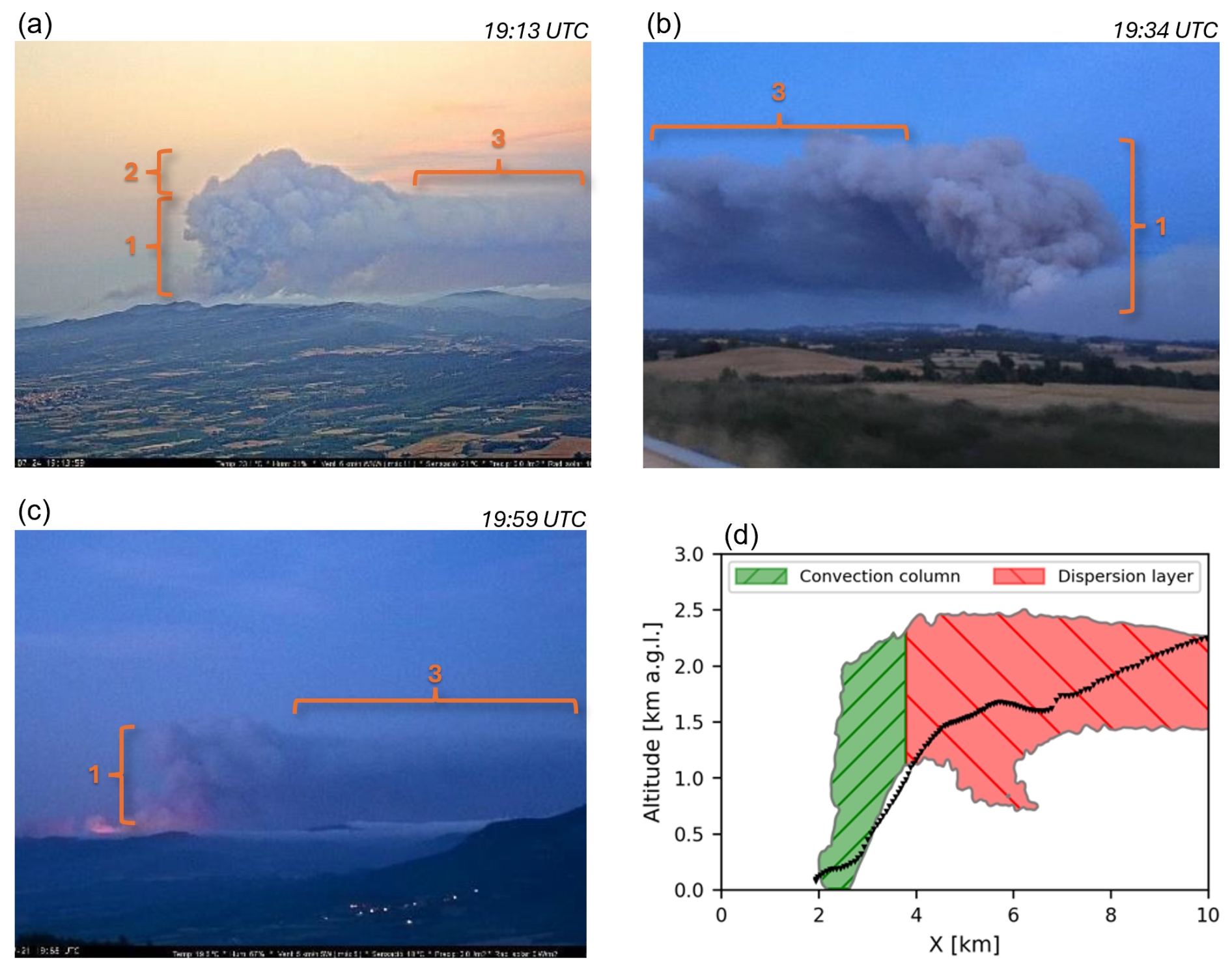
Figure 5 A qualitative comparison between the observed and simulated plume shape between 19:00–20:00 UTC. The observed plume is presented before sunset (19:41 UTC) at 19:13 (a) and 19:34 (b) and after sunset at 19:59 (c) UTC (LT−2) with the convection column, occasional overshooting and dispersion layer indicated by the numbers 1–3, respectively (Pictures taken from Ribau et al., 2022). The average simulated plume shape between 19:00–20:00 UTC (d) is visualised using the inert tracer (>0.0025) with green and red shading indicating the convection column and dispersion layer, respectivelly. Additionally, the displacement of the radiosonde in the east-west direction is shown (black triangles).

For the remainder of this comparison, we will compare the radiosonde measurements to the simulation, which has two challenges. Firstly, the location of the radiosonde relative to the plume during the measurements is unknown, as we do not have observations on the exact location of the plume during the sounding. Secondly, we cannot replicate the exact shape of the turbulent plume at the time of the sounding, since turbulence is a chaotic process. Instead, we can replicate the average shape of the plume between 19:00–20:00 UTC, the period in which the sounding was released. Despite these challenges, we know that the radiosonde moved predominantly eastward (Fig. 1a) and that it measured inside the convective core of the plume between 0.3–1.5 km altitude (Fig. 1b). To capture the convective core of the plume in the simulation, we extract a xz cross-section at y=12.8125 km. This xz cross-section represents an east-west plane through the centre of the fire, matching the predominant eastward movement of the radiosonde. Hence, we will compare the radiosonde measurements with the averaged xz cross-section of the plume in the fire-run between 19:00–20:00 UTC through the centre of the fire.

The measured rising speed and horizontal displacement of the in-plume radiosonde (black triangles; Fig. 5d) provide a quantification of the observed plume shape. The horizontal displacement of the radiosonde within the convective core of the plume (0.3–1.5 km altitude) shows that the averaged simulated plume shape is less tilted than the observed one. Above 1.5 km, the rising of the radiosonde effectively halts, resulting in approximately 3 km of primarily horizontal displacement between 1.5–1.7 km altitude before continuing its ascent (Fig. 5d). This suggests that the radiosonde exited the convection column between 1.5–1.7 km, but whether the exit occurred at the top of the plume cannot be derived from the rising speed and horizontal displacement of the radiosonde.

To further evaluate the simulated pyro-convection, we compare the simulated in-plume θ_v and U, with the radiosonde measurements during its ascent (black triangles; Fig. 6a and c). Additionally, we evaluate the simulated ambient conditions by comparing the observed θ_v during the descent of the radiosonde. The measurements near the surface (<0.3 km) during the ascent show an increase in θ_v (Fig. 6a). This increase coincides with the near-surface acceleration of the rising speed (Fig. 1b), which indicates that the increase in θ_v reflects the transition from the ambient atmosphere into the convective plume. Between 0.4–1.4 km, a relatively constant θ_v of 308 K is observed, which coincides with the observed convection column (i.e. where rising speed >2 m s⁻¹). Above the well-mixed layer, an inversion is found (1.7–1.9 km) with a stable layer on top (>1.9 km), which explains the predominantly horizontal displacement of the radiosonde for 3 km between 1.5–1.7 km altitude (Fig. 5d). The inversion is also visible in the measured U profile inside the plume (Fig. 6c). The U is relatively constant (5–10 m s⁻¹) up to 1.7 km above which it increases, indicating the transition from the atmospheric boundary layer into the free troposphere. The same inversion and stable layer are captured in the surroundings of the plume during the descent of the radiosonde (Fig. 6a).

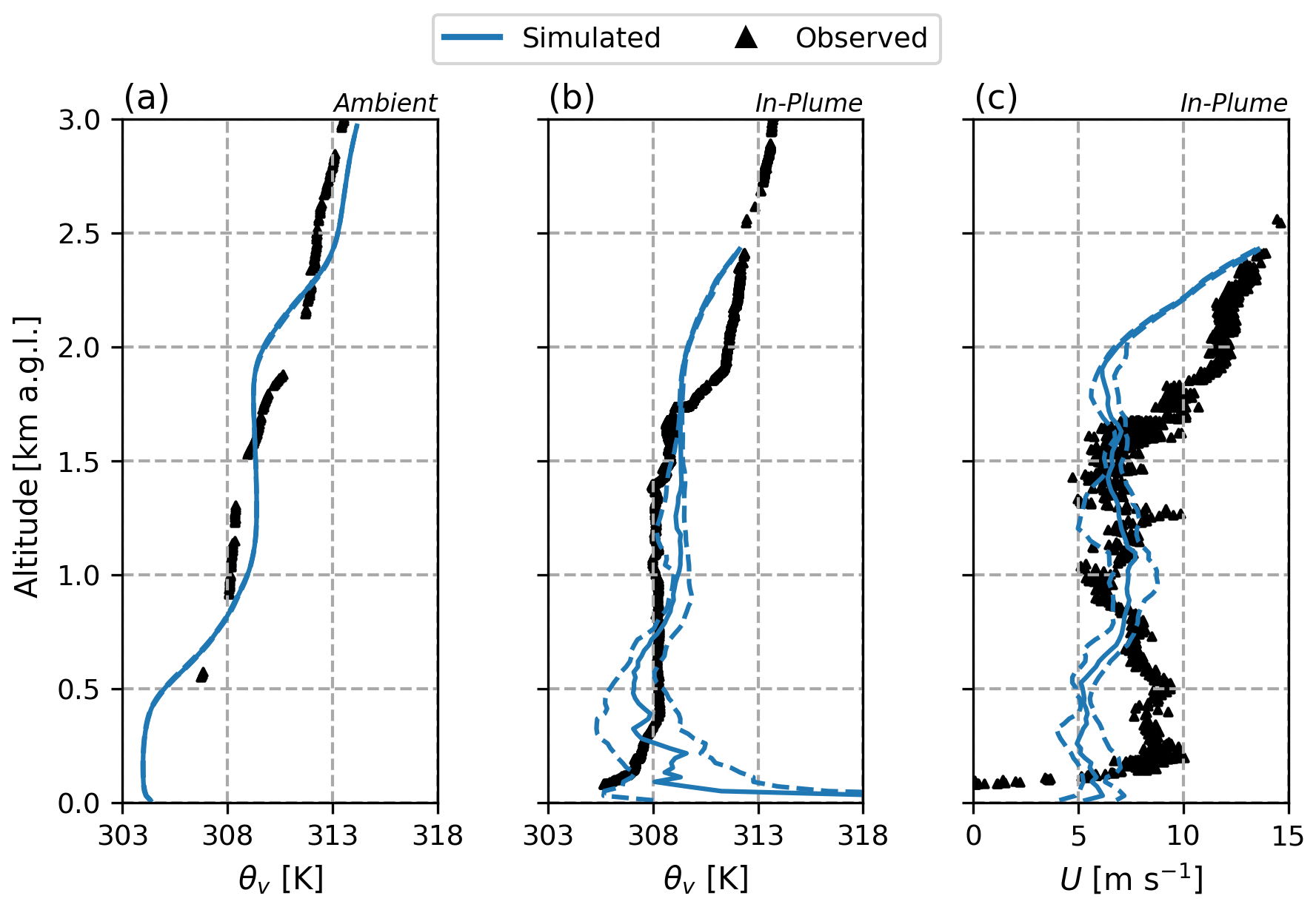
Figure 6 The vertical profiles θ_v measured during the descent (ambient conditions) and ascent (in-plume) of the radiosonde compared to the median simulated θ_v in the surrounding (a) and inside the average convection column (b) between 19:00–20:00 UTC. (c) The same as in (b) but for the measured and simulated wind speed, U. The first and third quantiles (blue dashed lines) indicate the simulated variability.

We compared the observations with the median θ_v and U profile (blue line) inside the average simulated convection column (Fig. 6). The medians of θ_v and U are determined per height inside the green-shaded area based on the averaged xz cross-section at y=12.8125 km. The spread in θ_v and U is indicated with the first and third quantiles (blue dotted lines). For consistency, the same approach is used to compare the measured and simulated ambient conditions surrounding the fire-induced plume, except for using the ref-run instead of the fire-run and the median based on the entire xz cross-section instead of the green-shaded area.

Figure 6b shows the median profile of θ_v inside the average convection column up to 2.3 km, which is the average height of the convection column between 19:00–20:00 UTC (Fig. 5d). At the surface (z=10 m), the median θ_v reaches 384 K (not shown), which quickly decreases due to mixing with the colder ambient air (304 K). This pattern is opposite to the sounding (black triangles), which shows a decrease in θ_v near the surface, because the simulated profile starts inside the flaming zone, whereas the radiosonde was launched outside the flaming zone.

Above the rapid decrease in θ_v, we find a well-mixed layer with a θ_v varying between 307–310 K in the simulation, which matches the observed mixed layer θ_v of 308 K (black triangles). However, the inversion capping the well-mixed layer is simulated ±0.3 km higher than observed (1.7 km). A similar overestimation is visible for the U profile. The simulated U is relatively constant up to 2 km altitude before increasing, indicating the presence of an inversion in the simulation at 2 km, while the observed U indicates an inversion at 1.7 km altitude.

The same difference in inversion height is present in the surroundings of the plume (Fig. 6a). The ambient conditions in the simulation are based on the ERA5 boundary conditions (Fig. 3), which also overestimate the inversion height by 0.3–0.4 km. Hence, the inversion height mismatch between the observations and the simulation (Fig. 6a) is created by ERA5 and does not reflect the performance of MicroHH. The overestimation by ERA5 is consistent with measurements in the same region and period of the SCQ fire presented by Mangan et al. (2023). They showed a consistent overestimation of the convective boundary layer by ERA5 due to its inability to capture local surface heterogeneity. At night, this would result in an overestimation of the height of the residual layer, which we find in Fig. 6a.

Due to the overestimated inversion height, we conjecture that the simulation also overestimates the plume height. A higher plume could amplify the impacts of wildfire-induced pyro-convection on the surrounding kinematic and thermodynamic structure of the atmosphere. Nonetheless, it is not expected to significantly alter the outcomes of this study. The simulation setup was inspired by the SCQ fire to ensure atmospheric realism and to capture the fire-induced circulation. As we demonstrate below, the simulation successfully replicates a fire-induced circulation (Sect. 3.2.1) as expected based on the observed surface wind reversal by the local fire fighters. Furthermore, the factors that govern the presence of a fire-induced circulation are located in the lowest 1 km above the surface (Sect. 3.2.2), far below the observed and simulated injection height of 1.7 and 2 km, respectively. Therefore, while the simulation does not perfectly replicate the meteorological conditions observed during the SCQ fire, it suffices for the objectives of this study: (1) quantifying the impact of a fire-induced circulation on the thermodynamic structure of the atmosphere and (2) identifying the factors governing the development of a fire-induced circulation.

3.2 Atmospheric response to dry pyro-convection

To explore the spatial impact of the simulated dry pyro-convection on the thermodynamic structure of the atmospheric boundary layer in the surroundings of the flaming zone, we calculated the boundary layer height (h) for the full 3D domain (Fig. 7). We know the ambient atmospheric boundary layer between 19:00–20:00 UTC consists of a neutral boundary layer ($\mathrm{0}<z<\mathrm{0.5}$ km) topped by a warmer and drier residual layer ($\mathrm{0.5}<z<\mathrm{2}$ km), which in turn is topped by an even warmer and drier free troposphere (Fig. 3a and b). Hence, we calculated h using the minimum $\frac{\mathrm{d}q}{\mathrm{d}z}$ between 0.1–1.6 km altitude (Fig. 7). The gradient in q identifies the interface between the relatively moist neutral layer and the drier residual layer (Fig. 3b), consistent with the mixed-layer framework described by Vilà-Guerau De Arellano et al. (2015). The altitude range is chosen to exclude the surface layer (z<0.1 km) and the capping inversion on top of the residual layer ($\mathrm{2}<z<\mathrm{2.5}$ km).

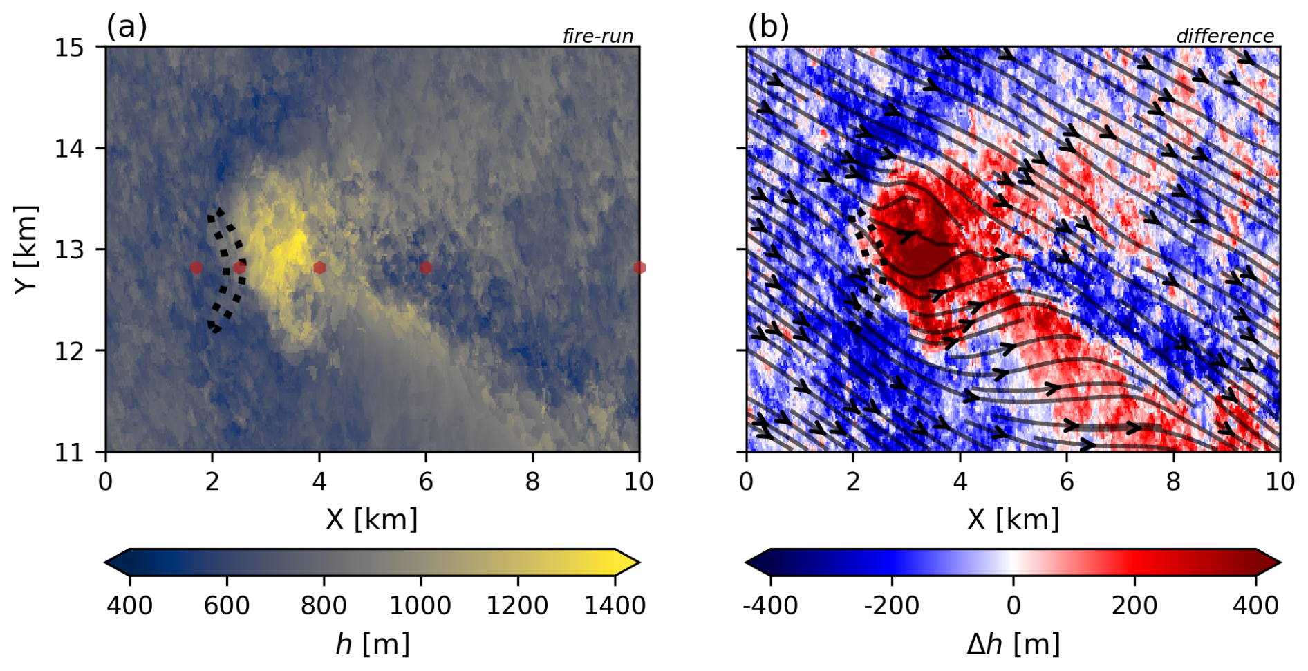
Figure 7 The average boundary layer height, h (a) between 19:00–20:00 UTC based on the minimum $\frac{\mathrm{d}q}{\mathrm{d}z}$ between 0.1–1.6 km altitude. The red hexagons from left to right represent the locations of the vertical profiles (a) to (e) in Fig. 8. To highlight the impact of the fire on h, we calculated the difference in h between the fire-run and ref-run (b). The black streamlines represent the average airflow in the residual layer based on the simulated airflow at 950 m altitude.

Figure 7 shows a decrease in h at the rear and the northern and southern flanks of the flaming zone (black dotted contour), whereas ahead (i.e. east) of the flaming zone, h increases within the first 2–3 km before it decreases. To investigate how these changes in h are reflected in the vertical structure of the atmosphere, we visualised the average vertical profile of θ_v between 19:00–20:00 UTC as a function of the eastward distance (x_ed; red hexagons in Fig. 7) from the fire (Fig. 8) for both the fire-run (orange line) and ref-run (blue dashed line). Here, the ref-run profiles represent the ambient conditions without a fire.

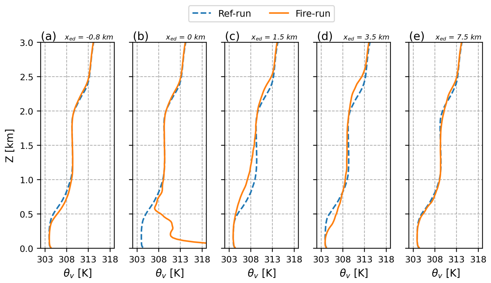
Figure 8 The average vertical profile of θ_v between 19:00–20:00 UTC for five eastward distances (x_ed) with respect to the head of the fire (x=2.5 km, y=12.8125 km): −0.8 km (a), 0 km (b), 1.5 km (c), 3.5 km (d), and 7.5 km (e). These five locations are visualised in Fig. 7a with red hexagons. To show the impact of the fire on the thermodynamic structure of the atmospheric boundary layer, the vertical profiles of θ_v for both the fire-run and ref-run are shown.

Directly above the fire (x_ed=0), the heating by the fire deepens the boundary layer from 0.5–2 km (Fig. 8b). West of the fire ($x_{\text{ed}}=-\mathrm{0.8}$ km), we find a slight decrease of the neutral boundary layer height (Fig. 8a). East of the fire, two opposite effects become apparent before the impact of the fire on the atmospheric boundary layer structure becomes negligible at x_ed=7.5 km (Fig. 8e). Near the fire (x_ed=1.5 km), the neutral boundary layer deepens (Fig. 8c), while further eastward (x_ed=3.5 km) the neutral boundary layer height is lowered from 0.5 to 0.25 km (Fig. 8d).

To understand the mechanisms behind these thermodynamic changes of the atmospheric boundary layer (Figs. 7 and 8), we analyse the modifications of the wind patterns by the fire in Sect. 3.2.1 and subsequently their connection to the thermodynamic changes in Sect. 3.2.2.

3.2.1 Fire-modified wind patterns

To investigate how the fire impacts its surrounding wind patterns, we compare the fire-run with the ref-run. The direct impact of any wildfire on the atmosphere is the creation of buoyancy by heating the air. With the fire, we find average vertical velocities up to 3 m s⁻¹ at the surface (Fig. 9b), an order of magnitude larger than the ambient vertical velocities (Fig. 9a). To sustain the increased vertical airflow above the flaming zone (black dotted line), additional inflow into the flaming zone is needed. Figure 9b suggests two mechanisms that could provide the additional inflow: (1) downdrafts at the southern and western borders of the flaming zone and (2) horizontal inflow from the western, eastern and northern borders (grey streamlines).

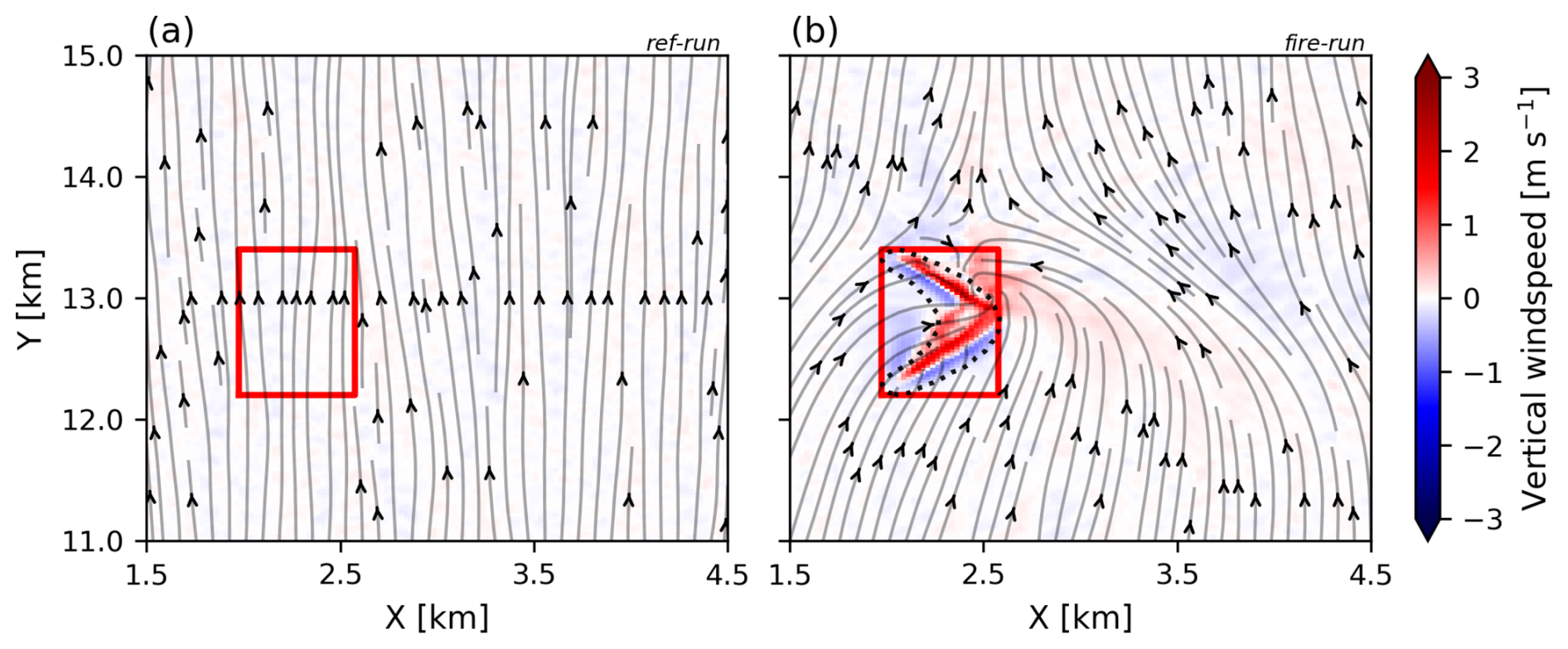
Figure 9 The average vertical wind speed in the ref-run (a) and fire-run (b) between 19:00–20:00 UTC at the lowest vertical level of the simulation (z=10 m). The grey streamlines show the hourly-averaged horizontal airflow patterns, the magnitude of which is presented in Fig. 11a and c. Furthermore, the red rectangle is the area for which we calculated the mass balance to quantify the influence of the fire on the surface winds (Fig. 10), and the black dotted line (b) indicates the simulated flaming zone (Fig. 2).

To quantify the change in airflow, we calculate the mass balance of the red box surrounding the flaming zone (Fig. 9) between 0–60 m altitude (Fig. 10). For the mass balance, we follow the mass conservation definition within MicroHH as defined in Eq. (2) in van Heerwaarden et al. (2017), which uses a reference density that is a function of height only. The limited altitude (<60 m) focuses the analyses on the near-surface layer below the plume neck.

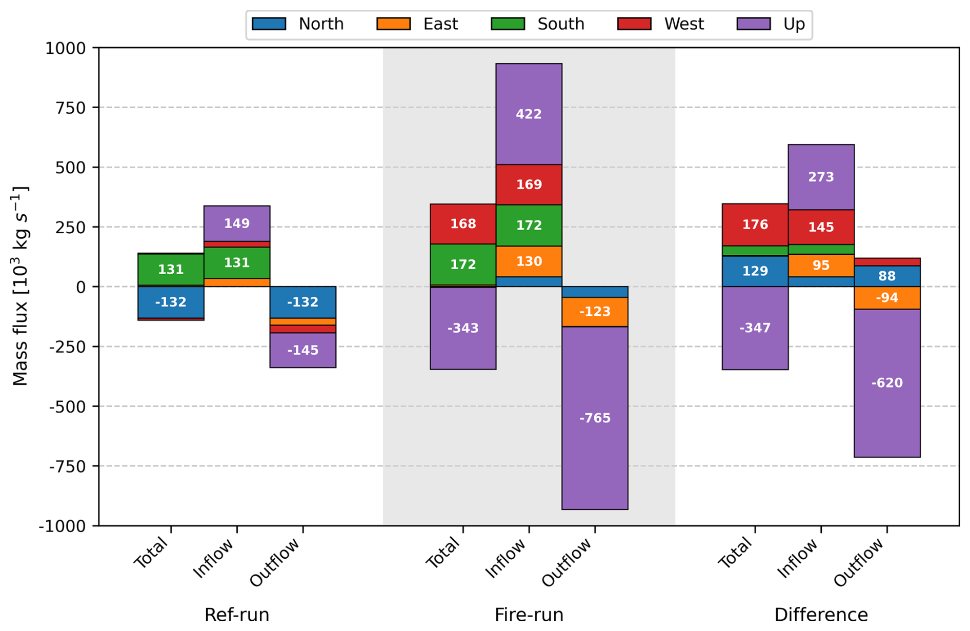
Figure 10 The mass flux balance for the ref-run and fire-run calculated over the boundaries of the red box in Fig. 9 in the lowest three layers of the simulation ($\mathrm{0}<z<\mathrm{60}$ m) between 19:00–20:00 UTC. The inflow (outflow) into the red box is defined as positive (negative). To investigate the impact of the fire on the mass transport, the difference between the two simulations (i.e. fire-run−ref-run) is shown.

Without a fire (ref-run), we find that the vertical in- and outflow are balanced (149×10³ and $-\mathrm{145}\times {\mathrm{10}}^{\mathrm{3}}$ kg s⁻¹, respectively). Additionally, as expected, the horizontal part of the mass flux balance of the ref-run is dominated by the southerly sea breeze, with predominantly inflow from the south (131×10³kg s⁻¹) and a nearly equal outflow in the north ($-\mathrm{132}\times {\mathrm{10}}^{\mathrm{3}}$ kg s⁻¹).

Comparing the ref-run with the fire-run in Fig. 10, we find a 620×10³ kg s⁻¹ increase in vertical outflow, which is partially compensated by a 273×10³ kg s⁻¹ increase in vertical inflow. The gap between the changes in vertical in- and outflow (347×10³ kg s⁻¹) is covered predominantly by changes in the airflow over the northern and western borders ($+\mathrm{129}\times {\mathrm{10}}^{\mathrm{3}}$ and $+\mathrm{176}\times {\mathrm{10}}^{\mathrm{3}}$ kg s⁻¹, respectively). At the northern border, the fire increases the inflow while decreasing the outflow, changing it from a net outflow border ($-\mathrm{132}\times {\mathrm{10}}^{\mathrm{3}}$ kg s⁻¹) to an almost net zero border. At the western border, the fire predominantly increases the inflow ($+\mathrm{145}\times {\mathrm{10}}^{\mathrm{3}}$ kg s⁻¹). Consequently, the net vertical outflow induced by the fire ($-\mathrm{343}\times {\mathrm{10}}^{\mathrm{3}}$ kg s⁻¹) is mostly compensated by southern (172×10³ kg s⁻¹) and western (168×10³ kg s⁻¹) inflow.

The total mass flux balance for the fire-run does not indicate a significant contribution from the eastern border, the front of the fire, despite the streamlines suggesting significant changes in airflow at the eastern border due to the fire (Fig. 9). This contradiction arises because both the in- and outflow at the eastern border increase equally, cancelling each other out in the total mass flux balance. To further analyse the airflow at the eastern border, we show the average zonal and meridional wind in Fig. 11 for the fire-run (a and c). Additionally, we show the difference between the fire-run and the ref-run (b and d) to highlight the acceleration and deceleration of the horizontal winds due to the fire. Figure 11b reveals two opposite changes at the eastern border: deceleration and acceleration of the zonal wind north and south of the centre of the fire (y=12.8125 km; purple dash-dot line), respectively. The combination of deceleration and acceleration explains the simultaneous increase in in- and outflow at the east border.

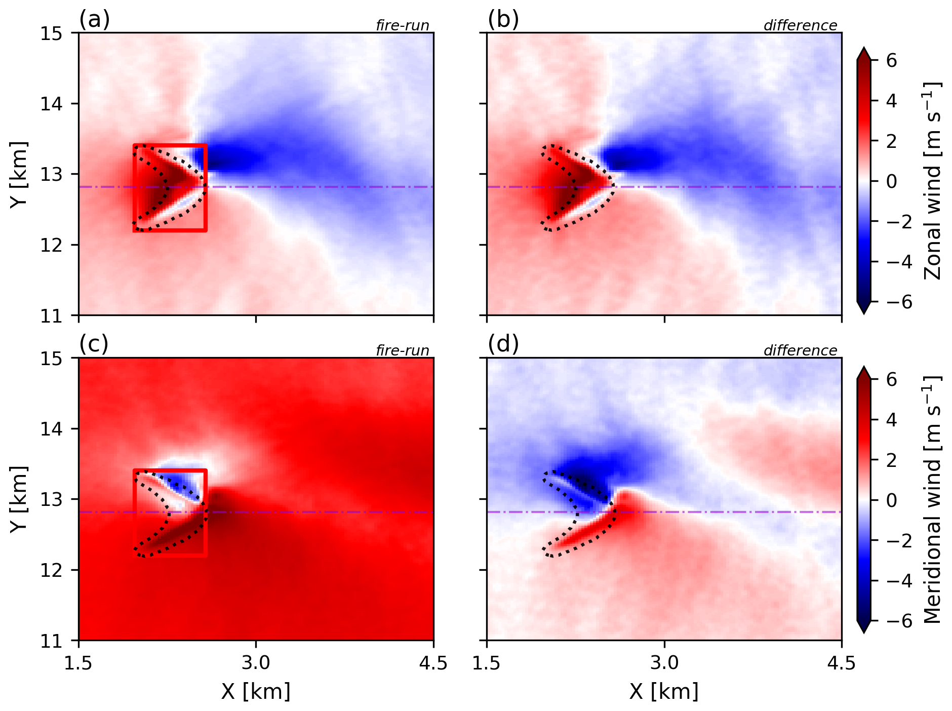
Figure 11 The average zonal (a) and meridional (c) wind between 19:00–20:00 UTC at the lowest vertical level of the simulation (z=10 m). To visualise the acceleration and deceleration due to the fire, the average difference between the fire-run and the ref-run is shown for both the zonal (b) and meridional (d) wind. The black dotted line and the purple dash-dot line indicate the simulated flaming zone (Fig. 2) and the centre of the fire (i.e. y=12.8125 km). The red rectangle shows the boundaries over which the mass flux balance in Fig. 10 is calculated.

Figure 12 shows the evolution of the surface wind patterns with altitude (Figs. 9–11). We limit ourselves to average east-west cross-sections since the simulated plume also developed to the east. The southerly winds at the surface (Fig. 3d) would suggest otherwise, but the westerly winds above 500 m altitude (Fig. 3d) result in the plume developing towards the east, similar to the observations described in Sect. 2.1. Hence, the east-west cross-sections are the most relevant for further analysis.

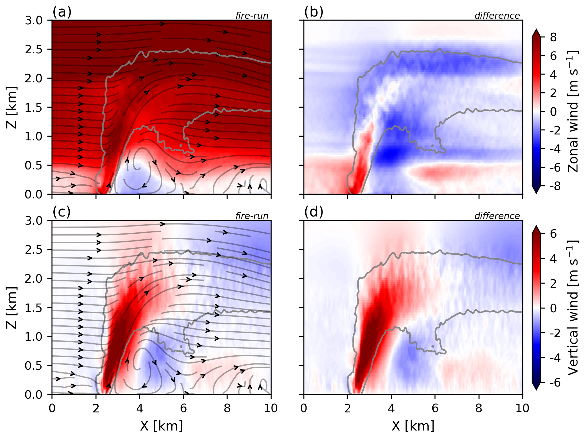
Figure 12 The vertical cross-sections of the average zonal (a) and vertical (c) wind between 19:00–20:00 UTC through the centre of the simulated fire (purple dash-dot line; Fig. 11). The grey outline and grey streamlines represent the average plume shape based on the inert tracer and the airflow through the cross-section. To visualise the acceleration and deceleration of the wind due to the fire, the average difference between the fire-run and the ref-run is shown for the zonal (b) and vertical (d) wind.

While both the acceleration and deceleration areas of the zonal wind extend up to 1.5 km altitude, their patterns differ (Fig. 12b). The acceleration occurs primarily inside the plume (grey outline), with the maximum acceleration at the surface. In contrast, the deceleration mainly occurs to the east of the fire (from x=2.6 km onward), with the maximum deceleration between 0.5–1 km altitude.

The largest impact on the vertical wind is the acceleration inside the plume (Fig. 12d), resulting in average vertical velocities up to 6 m s⁻¹ (Fig. 12c). We cannot directly compare the average simulated vertical velocities with instantaneous observations, which typically indicate vertical velocities of 10–30 m s⁻¹ (Banta et al., 1992; Lareau and Clements, 2017; Clements et al., 2018). The temporal averaging in Fig. 12 smooths away the instantaneous peaks in the simulated vertical velocities, resulting in relatively low average vertical velocities compared to instantaneous vertical velocities. In Fig. 13 we show the probability density function of the instantaneous vertical velocities inside the simulated plume (grey outline in Fig. 12) between 19:00–20:00 UTC for both the ref-run (blue) and fire-run (orange). When considering the instantaneous vertical velocities, we find updrafts up to 32 m s⁻¹, which matches the typical observed range of vertical velocities (Lareau and Clements, 2017; Clements et al., 2018). The same difference is visible between the average and instantaneous downdrafts. Averaged over time, the downdrafts peak at ±2 m s⁻¹ (Fig. 12c), while Fig. 13 shows that instantaneous downdrafts have velocities up to 10 m s⁻¹.

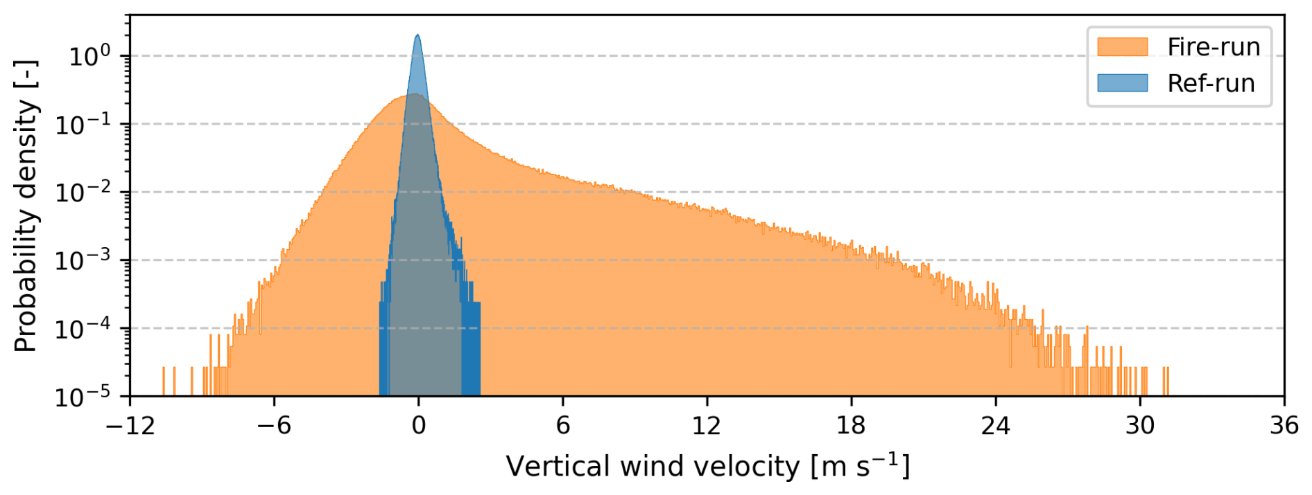
Figure 13 The probability density function of the instantaneous vertical wind inside the plume (grey outline in Fig. 12) between 19:00–20:00 UTC for both the ref-run (blue) and fire-run (orange).

The combined effect of these changes in the average zonal and vertical wind by the SCQ is visualised by the grey streamlines (Fig. 12a and c), which show the average airflow between 19:00–20:00 UTC. They reveal the formation of downdrafts 2 km east of the fire, in addition to the rising motions inside the plume. Between the up- and downdrafts, a fire-induced circulation is visible, consisting of negative zonal wind near the surface (z<0.5 km) and positive zonal wind aloft. Furthermore, the streamlines show descending inflow west of the fire (x<2 km) despite the relatively small negative average vertical velocities upwind compared to the downdrafts ahead of the fire (Fig. 12c).

3.2.2 Fire-modified boundary layer

To connect the fire-modified winds (Sect. 3.2.1) to the changes in the thermodynamic structure of the atmospheric boundary layer (Figs. 7 and 8), we show the average vertical cross-sections of the virtual potential temperature (θ_v) and specific humidity (q) during the fire-run in Fig. 14a and c combined with streamlines that represent the average airflow. Furthermore, to highlight the impact of the fire on the thermodynamic structure, Fig. 14b and d shows the difference in θ_v and q between the fire-run and the ref-run.

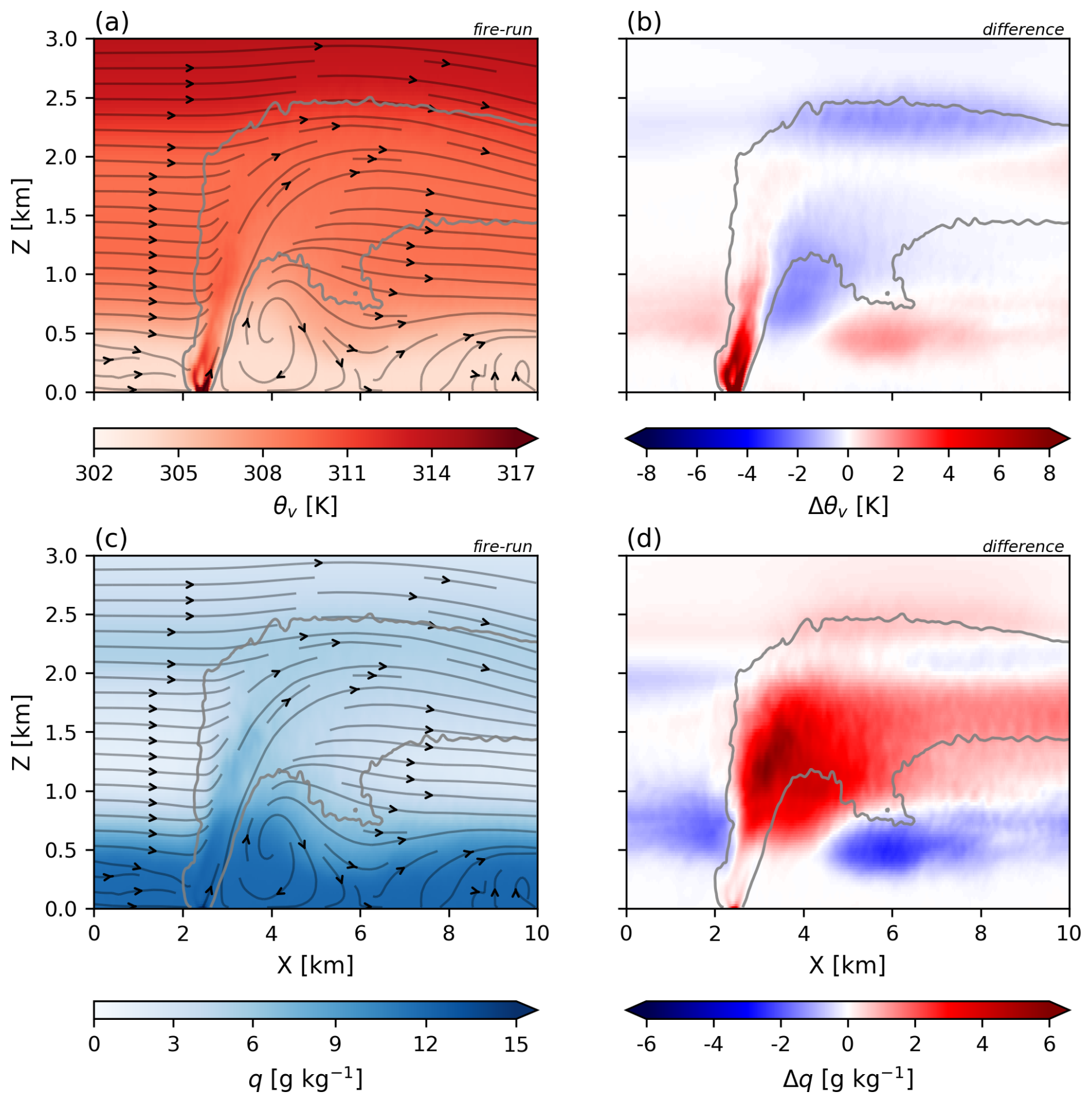
Figure 14 The vertical cross-sections of the average virtual potential temperature, θ_v (a), and specific humidity, q (c), between 19:00–20:00 UTC through the centre of the simulated fire (purple dash-dot line; Fig. 11). To highlight the impact of the fire, the average difference between the fire-run and the ref-run between 19:00–20:00 UTC is shown for θ_v (b) and q (d). The grey outline and the grey streamlines show the average shape of the simulated plume and the average airflow.

Inside the plume (grey outline), we observe heating near the surface (z<1 km; Fig. 14b), while moistening only begins above 0.5 km (Fig. 14d). This indicates that the fire directly affects θ_v through the sensible heat flux, while q is primarily affected indirectly through the upward transport of ambient moisture by the fire-induced convection.

East of the plume (x>2.6 km), two opposite patterns developed, matching the patterns of the boundary layer height in Figs. 7 and 8. Closest to the plume ($\mathrm{2.6}<x<\mathrm{4.5}$ km), Fig. 14b and d shows cooling and moistening in the lower part of the residual layer ($\mathrm{0.5}<z<\mathrm{1}$ km). Further eastward ($\mathrm{4.5}<x<\mathrm{8}$ km), the transition zone between the neutral boundary layer and the residual layer ($\mathrm{0.25}<z<\mathrm{0.75}$ km) is warmed and dried. These two opposite patterns reflect the interaction of the fire-modified winds (grey streamlines) with the ambient boundary layer structure surrounding the fire (blue dashed line in Fig. 8). Closest to the plume ($\mathrm{2.6}<x<\mathrm{4.5}$ km), the fire-induced circulation transports relatively cool and moist air from the neutral boundary layer into the residual layer above. Further eastward ($\mathrm{4}<x<\mathrm{6}$ km), the downdrafts transport relatively warm and dry air downward from the residual layer to the neutral boundary layer. A similar pattern of warming and drying, albeit less strong, is present west of the plume due to the descending rear inflow.

3.3 Sensitivity of the fire-induced circulation to wind shear

Figure 15 shows the vertical profiles of the zonal wind (u), meridional wind (v), wind speed (U) and wind direction (U_dir) for the fire-run (a-d) and the two sensitivity experiments: fire-run:no-u-advec (e-h) and fire-run:pg (i-l). As intended (see Sect. 2.3), the profiles show a decrease in directional wind shear due to reduced backing of the wind in the lowest ∼500 m. In both sensitivity experiments, the reduced backing is caused by an increase in u near the surface. The largest increase in u, and consequently the largest decrease in directional wind shear, occurs in fire-run:pg. The profiles of v and U in the sensitivity experiments remained relatively similar to the fire-run.

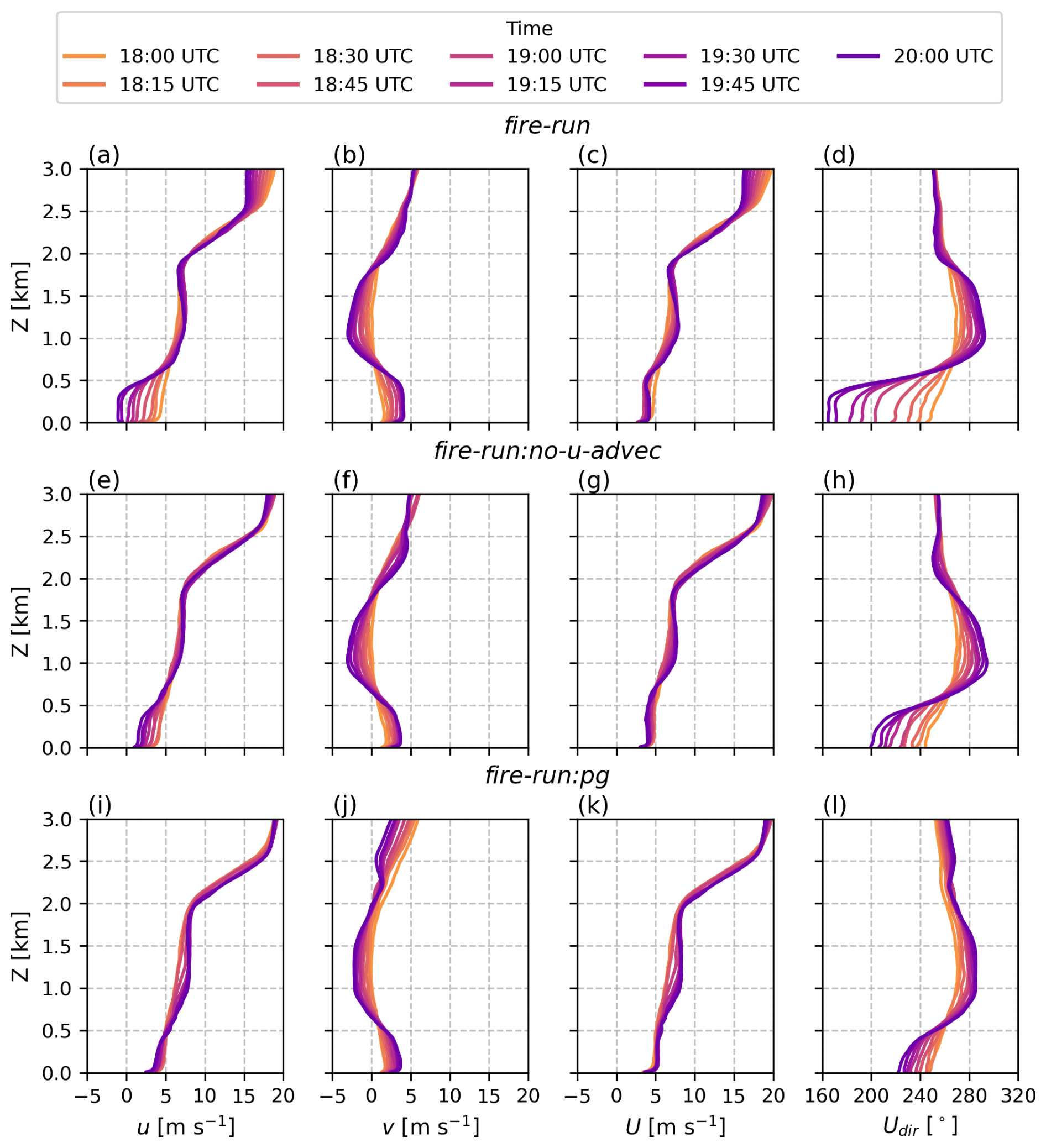
Figure 15 The vertical profiles of the zonal wind (u), meridional wind (v), wind speed (U) and wind direction (U_dir) between 18:00–20:00 UTC for the fire-run (a–d) and the two sensitivity runs: fire-run:no-u-advec (e–h) and fire-run:pg (i–l). The vertical profiles represent a line average along the x direction at y=12.8125 km.

In the following sections, we investigate how these changes in wind profiles modify the fire-induced circulation (Sect. 3.3.1) and subsequently whether these modifications alter the impact of the circulation on the thermodynamic structure of the atmospheric boundary layer (Sect. 3.3.2).

3.3.1 Fire-modified wind patterns

To analyse the impact of the changes in the vertical wind profiles (Fig. 16), we show the average zonal wind speed and streamlines in the horizontal cross-section directly above the surface at z=0.01 km (Fig. 16a–c) and the east-west cross-section through the flaming zone at y=12.8125 km (Fig. 16d–f). The experiments are ordered from left to right (a–c and d–f) by decreasing directional shear and increasing zonal wind speed (Fig. 15).

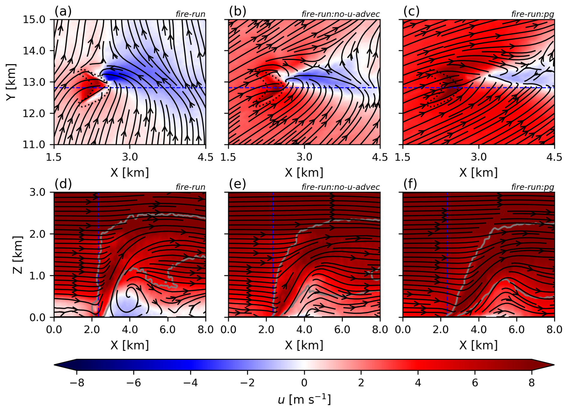
Figure 16 The average zonal wind speed (u) and streamlines in the horizontal cross-section directly above the surface (z=0.01 km) and the east-west cross-section through the flaming zone (black dotted contour) at y=12.8125 km (blue dashed line in panels a–c) between 19:00–20:00 UTC for the fire-run (a, d), fire-run:no-u-advec (b, e), and fire-run:pg (c, f). The experiments are ordered from left to right by decreasing directional shear and increasing zonal wind speed (Fig. 15). The blue dashed line in panels d–f shows the location of the north-south cross-sections in Fig. 17.

The horizontal cross-sections at the surface (Fig. 16a–c) show that increasing zonal wind speed and decreasing directional shear decrease both the magnitude and the spatial extent of the surface wind reversal (i.e. where u<0 m s⁻¹). Furthermore, in the sensitivity experiment with the largest changes in wind profiles, fire-run:pg, the starting point of the flow reversal is displaced approximately 600 m eastward compared to the other two experiments, where the flow reversal starts directly at the edge of the flaming zone (black dotted contour).

The east-west cross-sections (Fig. 16d–f) show that a clearly defined circulation is absent in the sensitivity experiments. Nonetheless, the updrafts between 2.6–4.5 km and the downdrafts between 4.5–6 km in the fire-run (d) still exist in the sensitivity experiments (e, f). The main difference with the fire-run is the decrease in magnitude and vertical extent of the reversed winds (i.e. where u<0 m s⁻¹) in the sensitivity experiments. Consequently, the flow reversal in the sensitivity experiments occurs only at the surface (<100 m), whereas in the fire-run the flow reversal extends to an altitude of 500 m. This difference suggests that the decrease in reversed surface winds in the sensitivity experiments disconnects the updrafts and downdrafts, thereby explaining the absence of a clearly defined circulation (e, f).

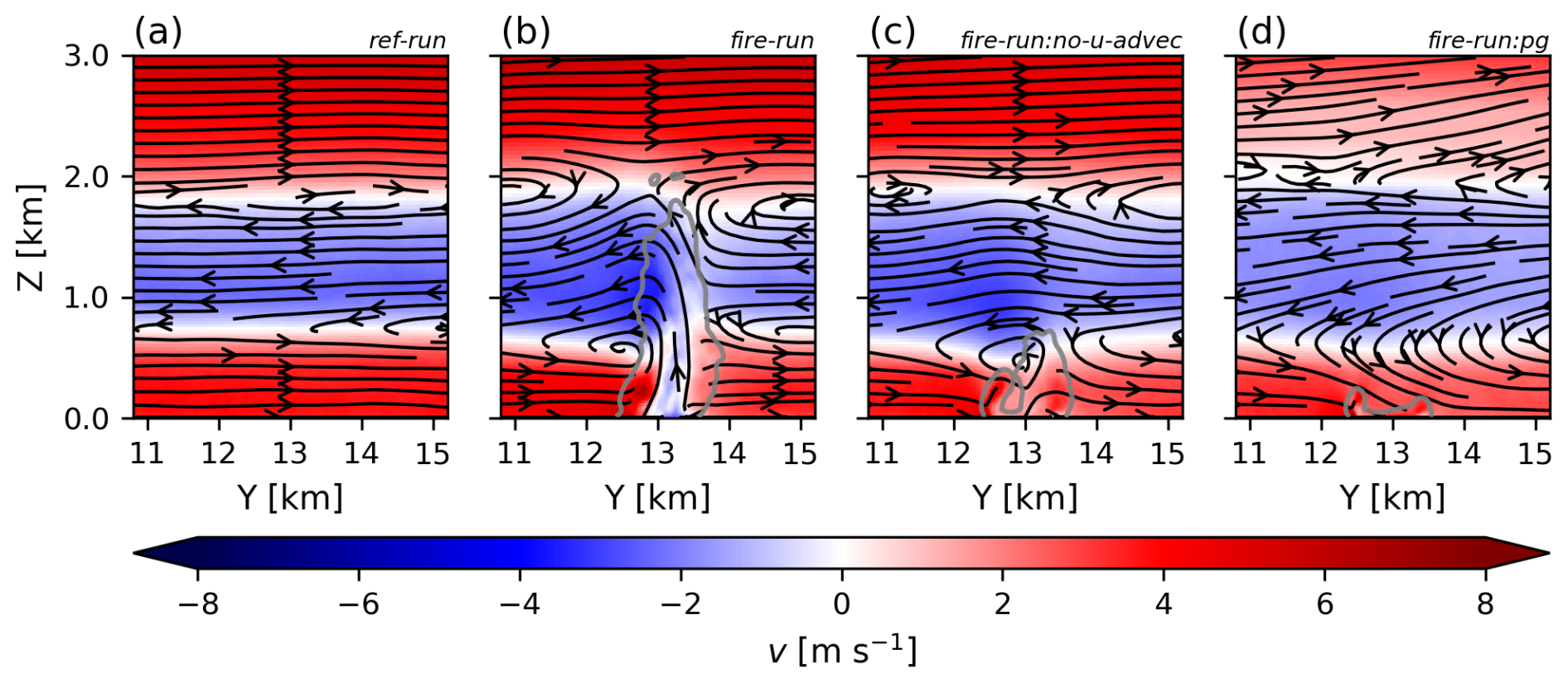
For completeness, we also show the average meridional wind and streamlines for the north-south cross-section (Fig. 17) for both the ref-run (a) and the three experiments with a fire (b–d) at x=2.35 km (blue dashed line in Fig. 16d–f). Matching the vertical profiles of v (Fig. 15b, f, and j), three distinct airflow layers are visible for all experiments: a positive v in the lowest 0.5 km, a negative v between 0.5–2 km, and a positive v again above 2 km altitude. Comparing the ref-run (a) and the three experiments with a fire (b–d), shows that pyro-convection strengthens the mixing between the layers, visualised by the circular streamlines at both sides of the plume (grey outline) around 0.75 and 2 km altitude.

Figure 17 The same as Fig. 16 (b–d), but for the meridional wind (v) in the north-east cross-section at x=2.35 km (blue dashed line in Fig. 16d–f) and including the ref-run (a).

3.3.2 Fire modified boundary layer

To visualise the impact of the fire-modified wind patterns on the thermodynamic structure of the ambient atmosphere for the different experiments, Fig. 18 shows the change in potential temperature between the experiments with fire and the ref-run for both the east-west and north-south cross-section (blue dashed lines in Fig. 16).

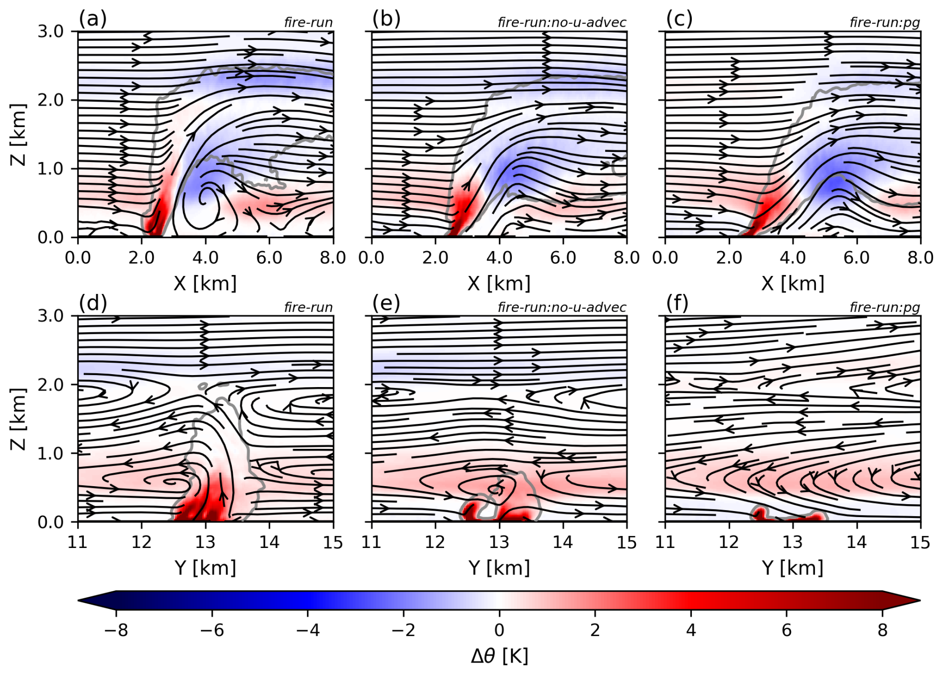
Figure 18 The average streamlines and difference in potential temperature with the ref-run in the east-west cross-section at y=12.8125 km (blue dashed line in Fig. 16a–c) and the north-south cross-section at x=2.35 km (blue dashed line in Fig. 16d–f) between 19:00–20:00 UTC for the fire-run (a, d), fire-run:no-u-advec (b, e), and fire-run:pg (c, f). The experiments are ordered from left to right by decreasing directional shear and increasing zonal wind speed (Fig. 15).

The impact of the fire-modified winds on θ in the sensitivity experiments is remarkably similar to the fire-run (a, d) despite significant changes in the zonal wind speed and the directional shear. At the surface, no significant changes in θ are found, while at higher altitudes, the same patterns in Δθ are visible.

The east-west cross-sections (Fig. 18a–c) show that, due to the persistence of the updrafts and downdrafts in the sensitivity experiment, the Δθ patterns are the same for all experiments. This persistence reveals that a full circulation ahead of the flaming zone is not necessary to get the same pattern of warming and cooling ahead of the flaming zone visible for the fire-run. Instead, two out of the three components that form the fire-induced circulation visible for the fire-run (a), the updrafts and downdrafts, must be present to create the cooling in the first 2 km ahead of the flaming zone and warming in the 2 km after.

In the north-south cross-sections (Fig. 18d–f), a warming and cooling tendency is visible around 0.75 and 2 km altitude, respectively. These tendencies coincide with the interfaces between the different airflow layers. Combined with the fact that θ increases with altitude in our simulations (Fig. 3a), these tendencies indicate that the mixing between the layers causes the downward transport of relatively warm air and the upward transport of relatively cold air around 0.75 and 2 km altitude, respectively.

4 Discussion

In this study, we investigated fire-induced circulations and their thermodynamic impact on the atmospheric boundary layer during dry pyro-convection using LESs inspired by the SCQ fire. In this section, we first provide a schematic overview to summarise the two distinct scenarios we found in our LES experiments (Sect. 4.1; Fig. 19). Next, we compare the wind patterns that form the fire-induced circulation with previous studies and discuss the mechanism causing the differences (Sect. 4.2). Lastly, we discuss the implications of the modified thermodynamic structure ahead of the flaming zone for dry convective fires such as the SCQ fire that inspired this study (Sect. 4.3).

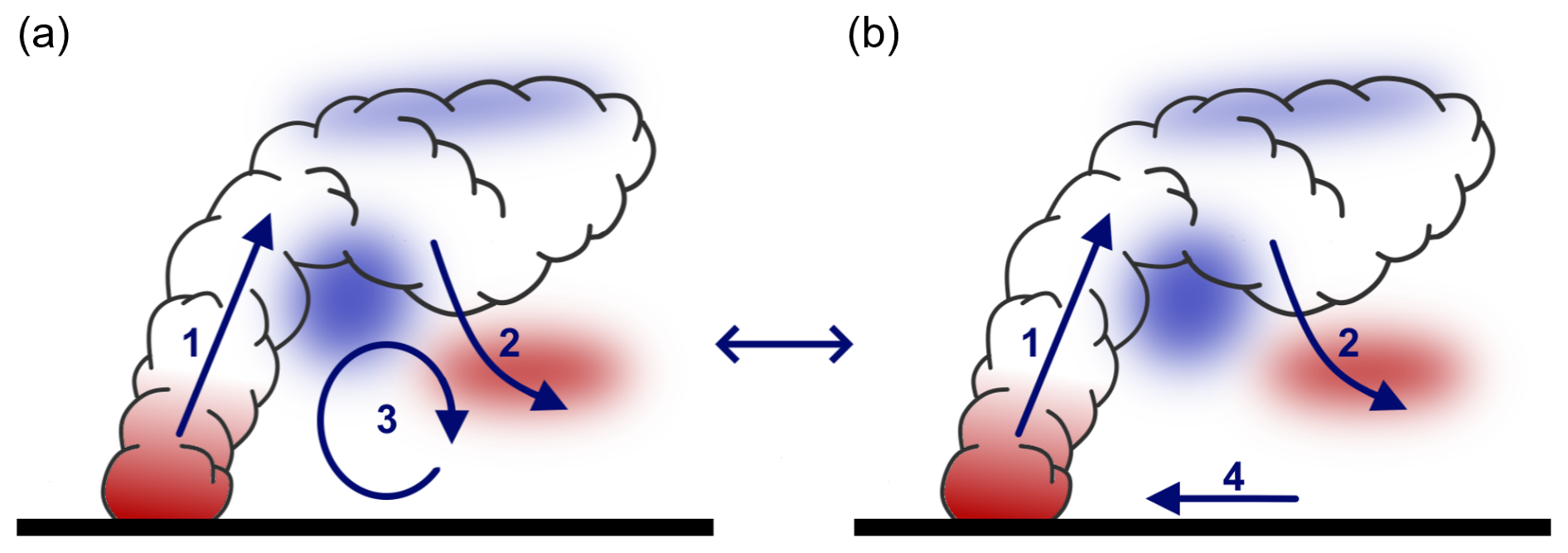
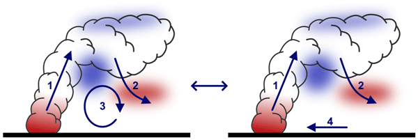
Figure 19 (a) A schematic overivew of the fire-modified wind patterns in the fire-run with: (1) convective motions inside the dry convective plume, (2) downdrafts ahead of the plume, and reversed surface winds connecting the downdrafts and updrafts into a circulation (3). To illustrate the impact of the fire on the thermodynamic structure in the fire-run, the blue and red shaded area represent the areas of warming and cooling compared to the ref-run. (b) The same schematic as in (a), but for the sensitivity experiments in which the magnitude and spatial extent of the reversed surface winds decreased. Consequently, we found that, instead of a clearly defined circulation, the three components of the circulation were disconnected: (1) the updrafts, (2) the downdrafts, and (4) the reversed surface winds. The schematics are based on Fig. 18a–c, but are not presented to scale.

4.1 Schematic overview of the results

Figure 19 shows the two distinct scenarios regarding the fire-induced circulation found in our LES experiments: one core simulation (fire-run) aimed at simulating the observed fire-induced circulations in realistic meteorological conditions and two sensitivity experiments designed to investigate the impact of the directional wind shear on the development of the fire-induced circulation. The core experiment produces a clearly defined circulation (Fig. 19a) comprised of three components: updrafts within the plume (1), downdrafts ahead of the plume (2), and reversed surface winds connecting the downdrafts and updrafts into a circulation (3). The sensitivity experiments generate the same three components; however, no coherent circulation develops (Fig. 19b). Despite the kinematic differences, all experiments produce identical thermodynamic impacts. Inside the plume (grey outline), all simulations show heating (red shading) near the surface and cooling at the top (blue shading). Ahead of the flaming zone, two opposite patterns are visible: cooling in the first 2 km followed by heating further eastward.

4.2 Fire-modified wind patterns

The circulation in our results (Fig. 19a) matches the observations by Banta et al. (1992) in both size and location. Based on Doppler measurements of the horizontal wind, Banta et al. (1992) suggested the presence of a persistent circulation ahead of the fire, which, similarly to our results, was observed in between the convective plume and downdrafts 2–3 km ahead of the fire. Furthermore, our simulations and the observations by Banta et al. (1992) both show downdrafts directed away from the circulation.

Regarding other simulation studies, our results align with those of van der Aa et al. (2026), who simulated the same fire. They show a circulation of similar spatial extent ahead of the fire, despite using a different LES framework. Furthermore, the simulations of a different fire by Filippi et al. (2018) also revealed a fire-induced circulation, albeit at the flank rather than at the head of the fire as seen in our simulation. Although the location differs from our simulation, the size of the circulation, approximately 1.5 km horizontally and 1 km vertically, matches our results.

Other observations (Lareau and Clements, 2017; Roberts et al., 2024) and simulations (Sun et al., 2009; Coen et al., 2013; Peace et al., 2016) of dry pyro-convection do not explicitly show a fire-induced circulation, but they do show the reversal of the surface wind. The reversed surface winds reported by these studies could indicate a fire-induced circulation (Fig. 19a); however, our sensitivity experiments show that reversed surface winds are not always part of a larger vertical structure (Fig. 19b).

In the sensitivity experiments, two factors changed simultaneously: directional wind shear decreases while zonal wind speed increases. We hypothesised that the directional wind shear is the primary driver of the circulation. However, based on the results, we expect that, contrary to our hypothesis, the zonal wind speed determines whether the circulation can develop for two reasons. Firstly, the directional wind shear decreased by 25 % and 50 % in the sensitivity experiment. If the directional wind shear were the primary driver of the fire-induced circulation, a proportional decrease in the magnitude and spatial extent would be expected. Instead, the circulation disappeared completely in both sensitivity experiments. Secondly, the main changes in the fire-modified wind patterns underlying the disappearance of the circulation were the reduction in spatial extent and magnitude of the reversed surface winds. The other two components of the circulation, the up- and downdrafts, were mostly unaffected in the sensitivity experiments. This reduction in reversed surface winds can be explained by the increase in zonal wind speed. The higher the zonal wind speed, the harder it becomes to create reversed surface winds, thus the smaller the area and magnitude of the reversed surface winds become.

This explanation also matches the purely theoretical discussion of dry convective plumes by Potter (2002), who start their reasoning with a simple case: a well-mixed atmosphere without ambient wind and a stationary heat source. Without wind, a plume rises vertically directly above the fire. To satisfy mass conservation, ambient air is drawn inward from all sides to compensate for this rising mass. This continuous updraft and corresponding lateral inflow trigger surrounding downdrafts, creating circulations on all sides of the fire (illustrated from a 2D perspective in Fig. 2 of Potter, 2002)

When wind is present, Potter (2002) argues the plume is tilted downwind, and with strong enough winds, the downdrafts and the reversed surface winds are disconnected from the flaming zone. With the sensitivity experiments, we capture this argument exactly. In fire-run:no-u-advec, the zonal wind speed increases to around 2 m s⁻¹ (Fig. 15e); the horizontal and vertical extent of the reversed surface winds decreases, but they still reach the fire. In contrast, with even higher zonal winds in fire-run:pg (4–5 m s⁻¹; Fig. 15i), the area with reversed surface winds is pushed eastward, causing a disconnect between the flaming zone and the reversed surface winds.

Besides providing a mechanism that governs the existence of the fire-induced circulation, our results also provide an explanation for the difference in location of the fire-induced circulation between our simulation (i.e. ahead of the fire) and the simulation by Filippi et al. (2018) (i.e. at the flank of the fire). In the simulation of Filippi et al. (2018), the wind was predominantly directed in the direction of the fire propagation. Consequently, the wind speed was higher along the direction of the fire propagation than across the fire front, the exact opposite of our core simulation (fire-run; Fig. 9). Hence, the formation of a fire-induced circulation at the flank in Filippi et al. (2018) fits our explanation; the relatively low wind speeds over the flanks allowed for sufficient reversal of the surface winds, thereby causing a circulation.

Similar to Filippi et al. (2018), Vaz et al. (2025) also shows the development of fire-induced circulations at the flanks, although their simulation includes pyro-cumulus formation, whereas our simulations and those of Filippi et al. (2018) do not. Nonetheless, the moment at which the circulations are shown by Vaz et al. (2025) coincides with the moment there is hardly any wind speed (∼0 m s⁻¹) aligned with the circulation, thus supporting our reasoning that the wind speed component aligned with the fire-induced circulation determines whether a circulation can develop. However, contrary to our arguments above regarding the theoretical discussion by Potter (2002), Vaz et al. (2025) argues that their findings do not align with Potter (2002) as their simulation includes a significant wind speed. We agree with Vaz et al. (2025) that there is significant wind (∼15 m s⁻¹ at the surface) in their simulations, but predominantly in the direction of the fire propagation. The circulations, on the other hand, occur at the flanks, in the direction without wind, which exactly fits the results from our sensitivity analysis and the theoretical discussion by Potter (2002).

Although our simulations provide insight into the mechanism that governs the presence of fire-induced circulation, future studies using non-stationary fires are required to investigate whether the presence of fire-induced circulations impacts fire behaviour. For example, radar observations show that reversed surface winds, the surface component of fire-induced circulations, coincide with the formation of fire-generated vortices (Lareau et al., 2022). This apparent correlation aligns with the operational experience of the Catalan Fire and Rescue Service, which suggests that reversed surface winds are typically associated with fire-generated vortices and long-range spot fires. To investigate these observations, two-way coupled fire-atmosphere simulations are required.

4.3 Fire-modified boundary layer

We studied the impact of the fire-modified winds (Fig. 19) on the surrounding thermodynamic structure of the atmospheric boundary layer to investigate whether dry convective fires such as the SCQ fire can counteract the cooling and moistening of the atmosphere at night ahead of itself. Warming and drying would explain the continued burning throughout the night of the SCQ fire, the fire that inspired this study. We found no warming or drying of the atmosphere at the surface due to the descending motions (Fig. 14). However, we did find two opposite changes in the boundary layer structure ahead of the fire (Fig. 8). Within the first 2 km ahead of the fire, we found a 40 %–60 % deepening of the neutral boundary layer. Further ahead, between 2–4 km ahead of the fire, we observed a 50 % decrease in boundary layer height.

Although the boundary layer height is not directly linked to fire behaviour, it is connected to plume growth. Generally, a higher well-mixed boundary layer is beneficial to plume growth. This suggests that when a dry convective fire, such as the SCQ fire, increases the boundary layer height within 2 km ahead of the fire front, it makes it easier for a fire to maintain a convective plume while advancing. We know from observations (e.g. Castellnou et al., 2022), that pyro-convection generally increases fire spread rates. Hence, we hypothesise that by modifying the boundary layer ahead, a fire can more easily sustain a convective plume, which subsequently promotes continued burning throughout the night, despite worsening burning conditions (i.e. cooling and moistening). The opposite applies when the boundary layer height is decreased; in that case, it becomes harder to sustain a convective plume, which is expected to decrease the ability of a fire to continue burning throughout the night.

This hypothesised impact on the fire behaviour only applies to fires that spread in the same direction as their plume, since that is the region where the boundary layer is modified. Hence, the hypothesis applies to the SCQ fire, since both the fire and plume spread eastward, which corresponds with the area where the boundary layer structure was modified in the simulation (Fig. 7). Visual observations suggest that the hypothesis is a plausible explanation for the continued burning until midnight by the SCQ fire, as the fire not only burned until midnight (22:00 UTC) but also maintained a convective plume throughout the night (Fig. 1a). With this explanation, we assume that the SCQ fire would continually deepen the boundary layer ahead while advancing forward.

A further complicating factor for predicting the impact of the fire-modified boundary layer on the fire behaviour is the formation of a surface inversion throughout the night. The surface inversion is not yet present in our LESs as we focused on the period (19:00–20:00 UTC) surrounding the shift from a positive to a negative surface heat flux (19:41 UTC). Consequently, there has been insufficient time for the formation of a surface inversion. We expect that the formation of a surface inversion would limit the ability of the fire to maintain a convective plume and subsequently limit the extent to which the pyro-convection can alter the thermodynamic structure of the atmosphere ahead of the fire. Simultaneously, it is unknown how the fire-modified winds would affect the surface inversion ahead of the fire. Hence, to test the hypothesis, further studies using a two-way fire atmosphere coupling are needed to investigate the extent to which a modified boundary layer structure explains continued nighttime burning during dry convective fires such as the SCQ fire.

5 Conclusions

For this study, we isolated the effects of dry pyro-convection on the atmosphere using LESs of stationary fires in realistic meteorological conditions inspired by observations from the SCQ fire. In total, we performed three simulations with a fire: a core simulation with a fire inspired by observations of the SCQ fire (fire-run), and two sensitivity experiments to isolate the impact of directional wind shear on the fire-induced circulation. As expected based on the observations of the local firefighters, the fire-run simulation reproduced a fire-induced circulation. Furthermore, the evaluation of the fire-run with visual plume observations and in-plume and ambient radiosonde measurements showed that our simulation setup sufficiently matched the observations for our objectives: (1) study the impact of the fire-induced circulation on the thermodynamic structure of the atmosphere ahead of the fire; and (2) explore which atmospheric factors govern the presence of the fire-induced circulation.

The fire-induced circulation in the fire-run was composed of three components: (1) updrafts in the dry convective plume, (2) downdrafts ahead of the plume and (3) reversed surface winds. We found no changes in surface temperature or humidity due to the circulation ahead of the fire. Hence, the hypothesis that the fire-induced circulation causes heating and drying near the surface is rejected. Instead, we found that the up- and downdrafts, two components of the circulation, modify the thermodynamic structure of the atmospheric boundary layer at higher altitudes (>0.25 km). The up- and downdrafts deepened the boundary layer over the first 2 km ahead of the fire, followed by 2 km of thinning.

Regarding the second objective, we originally hypothesised that directional wind shear governs the presence of a fire-induced circulation. To test this hypothesis, two sensitivity experiments were designed with an approximately 25 % and 50 % decrease in directional wind shear by increasing the zonal wind speed from 0 m s⁻¹ to 2 and 4 m s⁻¹. Already with a 25 % decrease in directional shear, the circulation completely disappeared, a disproportional change in wind patterns suggesting that, instead, the zonal wind speed governs the development of the circulation. The increase in zonal wind speed does explain the results, which showed that the decrease in spatial extent and magnitude of the surface wind reversal was the main reason behind the disappearance of the circulation. The higher the zonal wind speed, the component of the wind aligned with the circulation, the harder it is to reverse surface winds and create a circulation. Therefore, we reject our original hypothesis and propose a revised hypothesis: the wind speed component aligned with the circulation, rather than the directional wind shear, is the critical factor governing the presence of the fire-induced circulation.

In this study, we combined a stationary fire with a realistic atmosphere. While this approach successfully isolated the impacts of dry pyro-convection on the atmosphere under realistic atmospheric conditions, this approach also has its limitations. Firstly, we could not test the impact of the modified atmospheric boundary layer on the fire behaviour. Secondly, the realistic atmospheric conditions complicated the sensitivity analysis, as changing one wind component also changed the other wind components. Hence, for future work on fire-induced circulations, we propose two opposite directions away from our current approach: either increasing model complexity by including a two-way coupled fire spread model or decreasing complexity by using idealised meteorological conditions. The first pathway enables further understanding of how a fire-modified atmosphere affects the fire spread behaviour. In contrast, the second is focused on controlling all parameters of the simulation to isolate the processes governing the impact of pyro-convection on the surrounding atmosphere.

Appendix A: Validation of the periodic boundary conditions based on the specific humidity

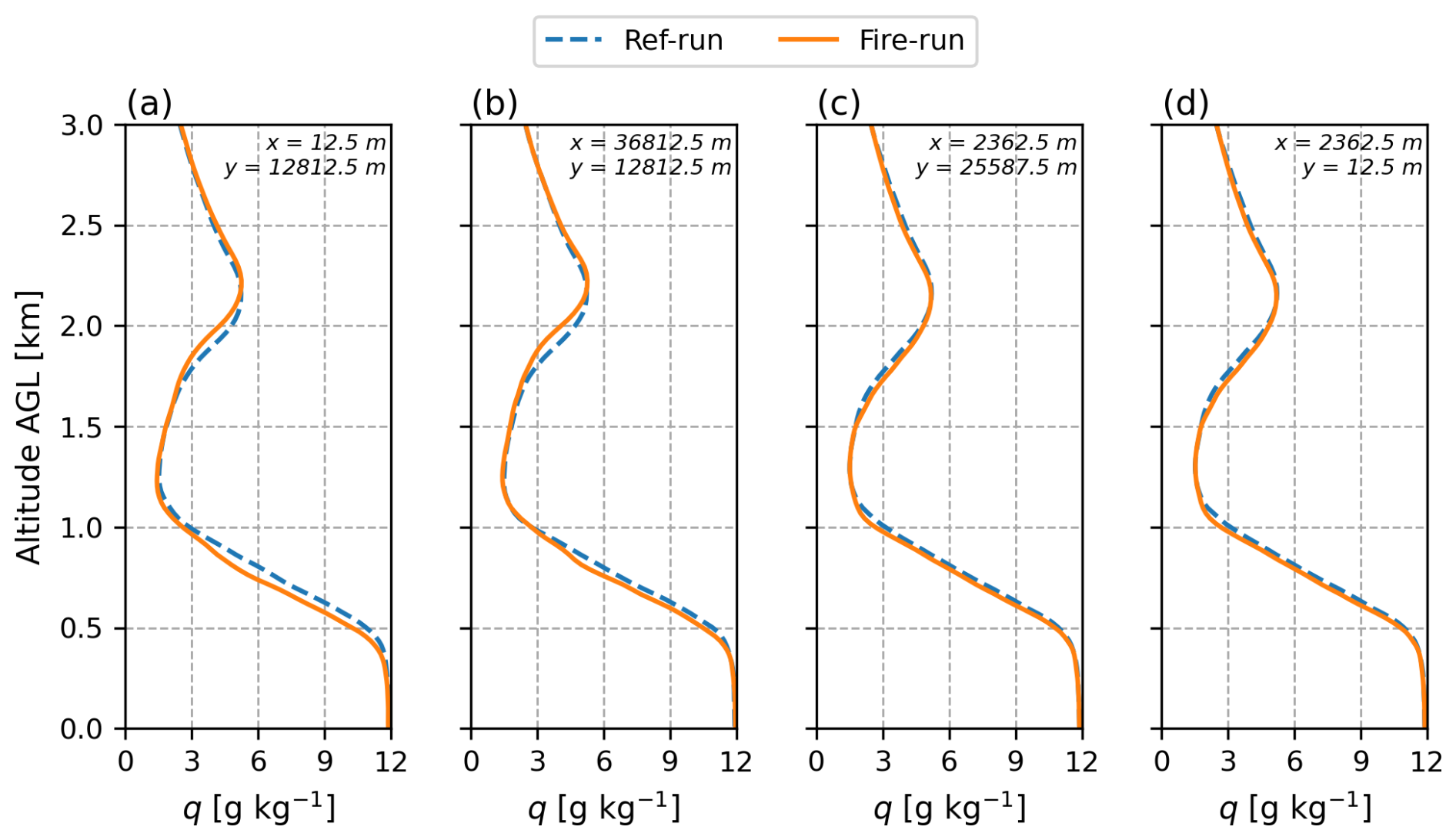
Figures A1 and A2 show the vertical profiles of the potential temperature (θ) and specific humidity (q) at each of the four borders of the simulated domain for both the ref-run (blue dashed line) and fire-run (orange line). There is no significant difference between the two simulations at any of the four borders of the domain, indicating the domain is sufficiently large to prevent any recirculation of the heat and moisture released by the simulated fire in the fire-run.

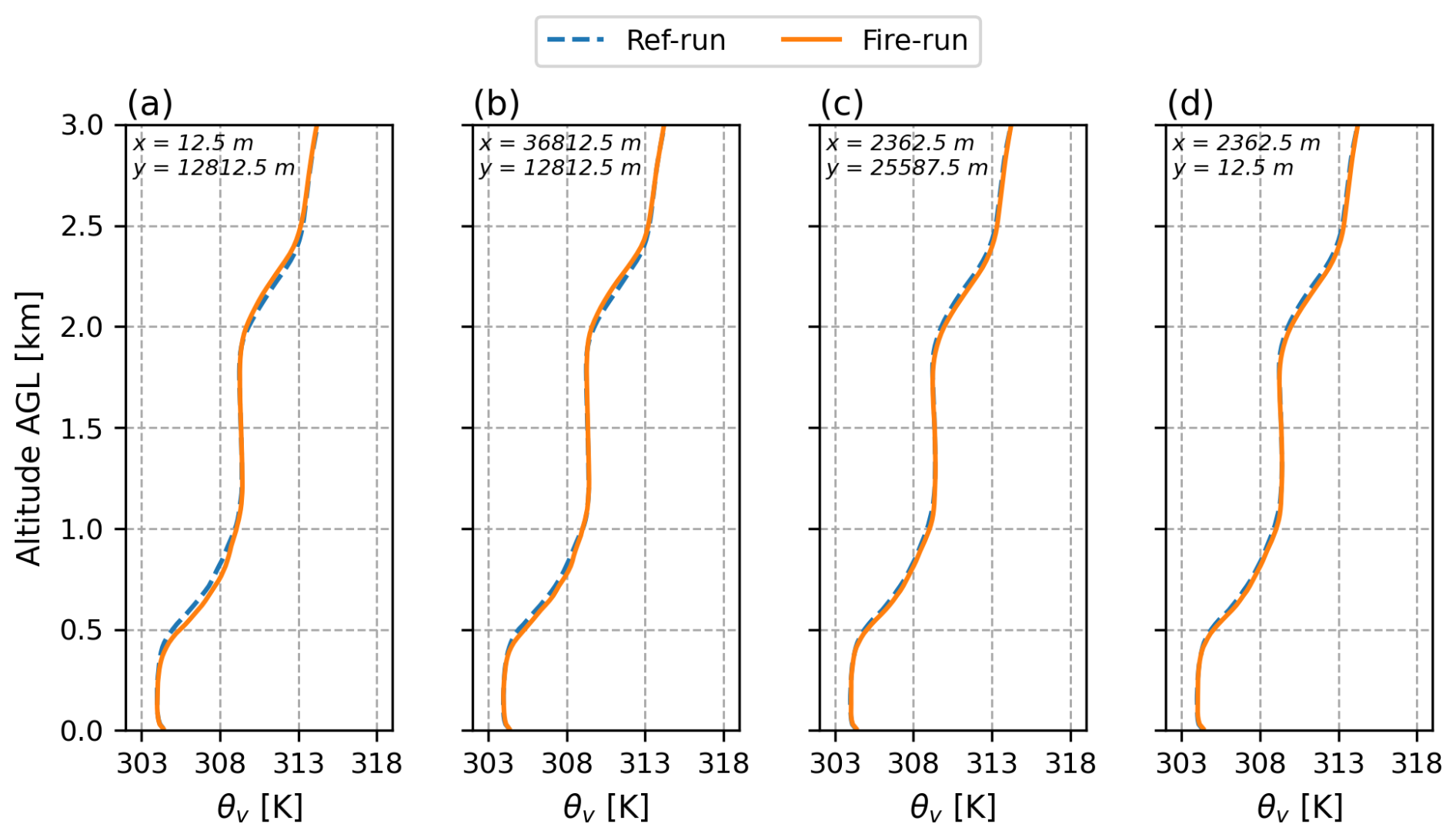
Figure A1 The averaged vertical profiles of θ_v between 19:00–20:00 UTC for the simulation without (ref-run; blue dashed line) and with fire (fire-run; orange line) at the four borders of the domain: west (a), east (b), north (c), and south (d). The x and y values on top of each column indicate the exact location of the vertical profiles following the coordinate system shown in Fig. 2.

Figure A2 The same as in Fig. A1, but for q instead of θ_v.