Urban surface-atmosphere fluxes of selected pptv-level oxygenated organic molecules (OOMs) from eddy covariance observations

Oxygenated Organic Molecules (OOMs) represent a substantial fraction of ambient reactive carbon and are potential precursors of secondary organic aerosols (SOA). Surface-atmosphere exchange flux modulates OOM budgets and subsequent SOA formation. This study presents the first urban eddy covariance measurements of pptv-level OOM surface-atmosphere fluxes, using an iodide-adduct chemical ionization mass spectrometer during the hottest month of the year in a central China megacity. We addressed the challenges of retrieving reliable fluxes for OOM species with low concentration signal-to-noise-ratios. Effects of mass spectral integration time and water vapor variation on flux estimates were investigated. We retrieved the fluxes of 16 OOMs, which displayed highly variable exchange behavior and fell into three categories: deposition-dominated, emission-dominated, and bidirectional exchange. Campaign-averaged daily deposition flux 4.6 µmol m⁻² d⁻¹ of 16 OOM was 16.3 % of HNO₃ deposition flux, but was higher than daily emission flux of OOMs by a factor of 2.2. Formic acid accounted for 66.2 % and 84.9 % of the summed deposition and emission fluxes of the 16 OOMs, respectively. Other appreciable contributors included isoprene-derived organonitrate C₄H₇NO₅, peracetic acid C₂H₄O₃, and nitrophenol C₆H₅NO₃. OOM fluxes at this urban site were generally lower than those previously reported above forest canopies, although the differences were typically within one order of magnitude. This work provides key methodological guidance and observational constraints for surface-atmosphere exchange of underrepresented reactive carbons.

1 Introduction

Oxygenated Organic Molecules (OOMs) are a group of low-volatility organic compounds typically containing 2–7 oxygen atoms. OOMs represent a substantial fraction of ambient reactive carbon and are potential precursors to secondary organic aerosols (SOA). Beyond atmospheric production and removal reactions, OOM budget in the atmosphere is modulated by complex surface-atmosphere exchange processes including surface emissions and dry deposition (Ehn et al., 2014; Fulgham et al., 2019). Currently, chemical transport models (CTMs) incorporate dry deposition schemes for only a very limited number of OOM, with deposition velocities poorly parameterized due to the lack of accurate effective Henry's law constants and surface reactivity data (Hodzic et al., 2013; Kelly et al., 2019; Wu et al., 2021; Zhang et al., 2003). This challenges accurate OOM budget estimates.

Direct OOM flux measurements, either emission or deposition, are essential for quantifying the atmospheric reactive carbon budget and constraining CTM predictions. The eddy covariance (EC) technique, the most accurate in-situ flux method, quantifies turbulent fluxes by measuring the covariance of vertical wind and concentration fluctuations. Many studies employed the EC technique coupled with proton-transfer-reaction mass spectrometry (PTR-MS) to measure VOC fluxes, primarily focusing on hydrocarbons (Fischer et al., 2021; Kim et al., 2017; Manco et al., 2022; Ruuskanen et al., 2011; Valach et al., 2015; Velasco et al., 2009; Vettikkat et al., 2023; Yuan et al., 2015; Zavarsky et al., 2018) and oxygenated VOCs (e.g., alcohols, aldehydes, and ketones; (Acton et al., 2020; Bachy et al., 2020; DiGangi et al., 2011; He et al., 2026; Hörtnagl et al., 2011; Karl et al., 2018). However, PTR-MS does not detect OOMs (e.g., organic acids, organonitrates, organosulfur compounds, hydroperoxides) that typically undergo bidirectional surface-atmosphere exchange.

Field-deployable negative-ion chemical ionization mass spectrometry (CIMS) (e.g., using I⁻, CH₃COO⁻, CF₃O⁻ ions) can detect OOMs, thereby enabling OOM flux measurement (Beaver et al., 2012; Bertram et al., 2011; Lee et al., 2014; Mattila et al., 2018). Despite these advances, most of existing studies focused only on formic acid (Fulgham et al., 2019; Gao et al., 2022; Nguyen et al., 2015; Schobesberger et al., 2016; Vermeuel et al., 2023) and peroxyacyl nitrates (PANs) (Min et al., 2012; Phillips et al., 2013; Turnipseed et al., 2006; Wolfe et al., 2009). Multi-species OOM flux measurements remain limited, and have been mostly conducted above forest canopies (Fulgham et al., 2019; Nguyen et al., 2015; Vermeuel et al., 2023).

Virtually no OOM flux measurements have been reported for urban environments, where governing factors of OOM fluxes (natural/anthropogenic emissions, near-surface chemical production and loss, and deposition resistance towards heterogeneous urban surfaces) are highly complex. Here, we deployed an iodide-adduct CIMS (I-CIMS) coupled with EC to measure surface-atmosphere fluxes of OOMs in an urban environment during the hottest month of a year. Unlike ppbv-level VOCs, OOMs typically occur at pptv or lower concentrations, and thus pose more measurement challenges (Langford et al., 2015). We specifically investigated optimized flux processing methods for the OOM with low signal-to-noise ratio (SNR) in their concentration measurements.

2 Methodology

2.1 Site Description and Eddy Covariance Measurements

Field measurements were conducted from 14 July to 10 August 2025 at a municipal air quality monitoring supersite on a university campus (114.6157° E, 30.4577° N) in Wuhan, a central Chinese inland megacity. A three-dimensional sonic anemometer (Campbell Scientific, CSAT3B) and an I-CIMS sampling inlet were mounted on a 10 m cylindrical mast atop the 20 m-high supersite building. The site is surrounded by wooded areas in the southwest and northeast, and a mixed building-tree campus landscape in other directions, with surrounding buildings averaging 15 m in height. Because detailed wind-sector-resolved building and vegetation morphology was unavailable, wind-direction-dependent displacement heights were not prescribed. A single representative zero-plane displacement height of d=10 m (0.67 × 15 m) was used (Arya, 1988; Stull, 1988; Oke, 1987), where the mean height of the surrounding buildings 15 m was adopted as a representative roughness-element height. Flux footprint analysis (Fig. S1 in the Supplement) indicates that 90 % of the measured fluxes originated from within 500 m of the supersite. The site was characterized by summertime biogenic emissions from vegetation overlapped with potential urban anthropogenic sources. The campaign covered the annual peak of temperature, humidity, solar radiation and atmospheric oxidation capacity in Wuhan; short rainfall events were excluded from flux analysis. Therefore, the observed OOM fluxes should be regarded as representative of summertime surface-atmosphere exchange rather than annual behavior.

The horizontally mounted, west-facing sonic anemometer recorded 3D wind components and sonic temperature (T_s) at 10 Hz, with negligible flow distortion from the slender mast. The I-CIMS inlet was set 0.23 m below and 0.85 m east of the sonic sensor to minimize sensor separation. Following Fulgham et al. (2019) and Vermeuel et al. (2023), who used long PFA/FEP tubes to sample atmospheric OOMs from flux tower tops, we drew ambient air through a 20.8 m-long, $\mathrm{3}/\mathrm{8}$ in. ID PFA tube at 80 slpm (standard liter per minute), corresponding to a nominal residence time of approximately 1.1 s and turbulent flow, to the I-CIMS housed in an air-conditioned room on the building's top floor. A schematic of the observation system is provided in Fig. S2. The indoor segment of the PFA tube was heated to 40 °C to minimize wall interactions, water vapor condensation and sample flow temperature fluctuations. Reversible adsorption/desorption of OOMs on PFA tubing surfaces has been documented (Liu et al., 2019; Nguyen et al., 2015), primarily causing high-frequency flux attenuation while largely preserving bulk concentrations. To assess potential concentration losses in our inlet, six compounds formic acid, acetic acid, lactic acid, pimelic acid, erythritol, and 4-nitrophenol, which are themselves target OOMs with measurable fluxes at this site or structurally similar surrogates of target OOMs, were measured under two sampling configurations: direct introduction into the I-CIMS and introduction through the 20.8 m PFA tube. The resulting signal changes range from −3.39 % to +0.30 %, indicating negligible concentration loss. Therefore, no concentration correction was made. Regarding flux loss, low-pass spectral correction (Ibrom et al., 2007) was adopted to correct high-frequency flux attenuation (discussed in Sect. 3.1).

The I-CIMS operated at 1.8 slpm to measure iodide adducts of OOMs and inorganic species (e.g., HNO₃) at 10 Hz. A 36 min measurement cycle was applied, including 31 min for ambient sampling and 5 min for high-purity nitrogen blank correction. For each measurement cycle, one flux estimate was calculated using the 10 Hz data from a continuous 30 min window within the 31 min ambient sampling period. Thus, the flux averaging period was 30 min, whereas the measurement cycle was 36 min, yielding up to 40 flux estimates per day under continuous operation. Air temperature and relative humidity were monitored at 1 Hz at the inlet of I-CIMS. Sonic and I-CIMS datasets were independently collected with unified time synchronization. After strict quality control, valid data of 28 d were used for flux analysis.

2.2 I-CIMS data processing

2.2.1 Peak fitting of target OOMs

After mass calibration and peak fitting of raw mass spectra, exact peak masses were matched to plausible chemical formulas C_1–30H_1–60O_0–20N_0–2S_0–2I${}_{\mathrm{0}\text{–}\mathrm{1}}^{-}$ under elemental ratio constraints. Mass assignment was performed with a mass error < 10 ppm at MS resolution of ∼ 6000. Priority was given to elemental formulas corresponding to atmospherically relevant OOM species reported by previous studies. This workflow identified over 400 ion formulas, whose 10 Hz time series were normalized to one million reagent ions (total I⁻ and IH₂O⁻) (Text S1 in the Supplement).

The SNRs for the 10 Hz ion signals were calculated over 30 min intervals and averaged to obtain mean SNRs for 0.1 s integration time. Only iodide-adduct ions with mean SNR > 2 were retained as target ions; this threshold corresponds to an SNR > 18 for 1 min integration time, which was commonly reported in concentration measurements. The retained ions were therefore also those with the high signal intensities. The target ions suffering from severe interference by adjacent peaks were also discarded. In total, 21 target OOMs, in the form of iodide-adduct ions shown in Table S1 in the Supplement, were selected for a second run of peak fitting to produce refined 10 Hz time series, which were used for subsequent spectral evaluation and flux analysis.

2.2.2 Calibration of OOM Mixing Ratios

Authentic standards are unavailable for most OOM species detected by the I-CIMS, making compound-specific calibration infeasible. In this study, OOM response factors were quantified via a collision-limited sensitivity calibration method (Isaacman-VanWertz et al., 2018; Lopez-Hilfiker et al., 2016; Ye et al., 2021; Song et al., 2024; Wang et al., 2026) from three components: (1) maximum instrumental sensitivity (S_max), referring to the sensitivity of compounds forming M ⋅ I⁻ adducts (where M denotes the neutral target analyte molecule and I⁻ denotes the iodide reagent ion) at the collision limit, (2) the relative sensitivity of M ⋅ I⁻ adducts ($\mathrm{1}/S_{\mathrm{0}}$) due to partial declustering in the electric fields, and (3) mass-dependent transmission efficiency (T_M) of M ⋅ I⁻ adducts relative to I⁻ reagent ion within ion optics and detector. S_max under dry-air conditions was calibrated using levoglucosan, a reference compound forming M ⋅ I⁻ adduct at collision limit. The levoglucosan S_max checks performed every two days showed only small variations throughout the campaign (< 2.6 %), indicating that the I-CIMS sensitivity remained stable during the campaign. The full workflow for determining response factor ($S_{\max }\times \frac{\mathrm{1}}{S_{\mathrm{0}}}\times T_{\mathrm{M}}$, units: cps pptv⁻¹) is presented in Texts S2–S4. The overall calibration uncertainty of this method is estimated to be 33 %–65 % (2σ, 95 % confidence interval), varying with the target species (Text S6). To validate the approach, direct calibrations of HNO₃ and formic acid using certified Kintek permeation tubes yielded dry-condition sensitivities of 25 and 36 cps pptv⁻¹, respectively, which fall within the ± 33 % of the HNO₃ and formic acid response factors derived from our collision-limited sensitivity method (detailed calibration procedure in Text S5).

The effect of humidity on I-CIMS sensitivity was determined using seven surrogate compounds (nitric acid, formic acid, lactic acid, acetic acid, 4-nitrophenol, pimelic acid, and erythritol (Text S6). The result of ambient humidity correction factors (RH_corr) relative to the sensitivity under dry-air conditions is further discussed in Sect. 3.2.2. Humidity corrected response factors of All target OOM are listed in Table S1.

2.3 Eddy Covariance Data Processing and Quality Control

Under the assumptions of negligible horizontal and vertical advection, the EC flux F is defined as:

$$\begin{array}{}\text{(1)}& F={\mathit{\rho }}_{\mathrm{d}}\stackrel{\mathrm{‾}}{w^{\prime }{c}^{\prime }}\end{array}$$

where ρ_d is the dry air density, w^′ is the fluctuation in vertical wind speed, and c^′ is the fluctuation in OOM dry mole fraction. Prior to eddy covariance flux calculations, all 10 Hz raw data (wind components, T_s, c) were standardized preprocessed using EddyPro 7.0 software, including geographic yaw correction, double rotation for tilt/terrain bias removal, and Vickers and Mahrt (1997) quality control (despiking + statistical screening). Invalid 30 min intervals with failed critical variable flags were excluded (Text S7).

To correct tube transport delay in the closed-path system, actual lag times between gas concentrations and vertical wind speed were determined using the maximum cross-covariance method (Text S8). In practice, the signals of some low-SNR OOM may cause noise-induced mismatches between 10 Hz concentration and wind speed data, introducing uncertainties in species-specific lag time derivation. Following Fares et al. (2012), we assumed identical turbulent transport for all species passing through the same sampling tube. This assumption is partly supported by our direct lag-time measurements using brief pulses of gaseous nitric acid, formic acid, and acetic acid standards introduced at the inlet of the 20.8 m PFA tube; despite their different chemical properties, the three compounds showed essentially identical transport delays (Fig. S5). HNO₃, with the highest SNR, was selected as the reference tracer, and its 30 min lag times were uniformly applied to all OOMs. This approach reduced random errors for low-SNR OOMs and improved time alignment accuracy for flux calculations. The HNO₃ lag times exhibited a mean diurnal value of 1.72 ± 0.88 s (Fig. S6).

After lag time correction, a 250 s moving average detrending was applied to the 10 Hz raw data for each 30 min interval to remove low-frequency non-turbulent trends from diurnal cycles, synoptic weather processes, and background signal fluctuations. Raw fluxes were then calculated per Eq. (1).

All 30 min fluxes were quality-screened via the steady state test (SST) and integral turbulence characteristic (ITC) test per Foken et al. (2004). These tests assess covariance stationarity across sub-intervals within 30 min and agreement between measured dimensionless concentration variances and Monin-Obukhov similarity theory (MOST) predictions, respectively, producing quality flags (Text S9). Fluxes failing these tests were excluded from further analysis.

Friction velocity (u^*) and Monin-Obukhov stability parameter ($z/L$) were also used to assess data quality. Over the campaign, 86 % of the 30 min u^* values exceeded 0.2 m s⁻¹, indicating well-developed turbulent mixing. $z/L$ ranged from −2 (strongly unstable) to slightly positive values (weakly stable).

Random sampling uncertainty in 30 min eddy covariance fluxes, arising from the stochastic nature of turbulence and the finite number of independent turbulent realizations sampled within each averaging period, was quantified using the method of Finkelstein and Sims (2001) (Text S10). The method is based on the variance of a covariance between vertical wind velocity and scalar concentration, which are auto- and cross-correlated. The resulting standard error σ_F defines a ∼ 68 % confidence interval (F ± σ_F) around each flux estimate. Flux detection limits, set at 2σ_F for all species, are provided in Table S1.

3 Results and discussion

3.1 Spectral analysis and flux loss correction

Spectral analysis is critical for assessing turbulence data quality, validating flux consistency, and diagnosing system high-frequency response limitations. The mean SNRs of the 10 Hz ion signals for the target OOMs range from 2.1 to 9.9 in the campaign, corresponding to 19–63 at 1 min integration time. Such low SNRs at 0.1 s integration time were also reported by prior EC flux studies of OOM or OVOCs (Coggon et al., 2021; Nguyen et al., 2015; Yang et al., 2013). To examine how spectral behavior varies with SNR, we selected four representative species spanning the observed SNR range: high-SNR HNO₃ (9.9), medium-SNR C₄H₇NO₅ (5.6) and CH₂O₂ (3.6), and low-SNR C₃H₄O₄ (2.2), all at 0.1 s integration time. Power spectra (w, T_s, HNO₃/OOMs) and cospectra (w-T_s, w-HNO₃/OOM) were computed via Fast Fourier Transform from 30 min 10 Hz fluctuation time series and averaged into logarithmically spaced frequency bins.

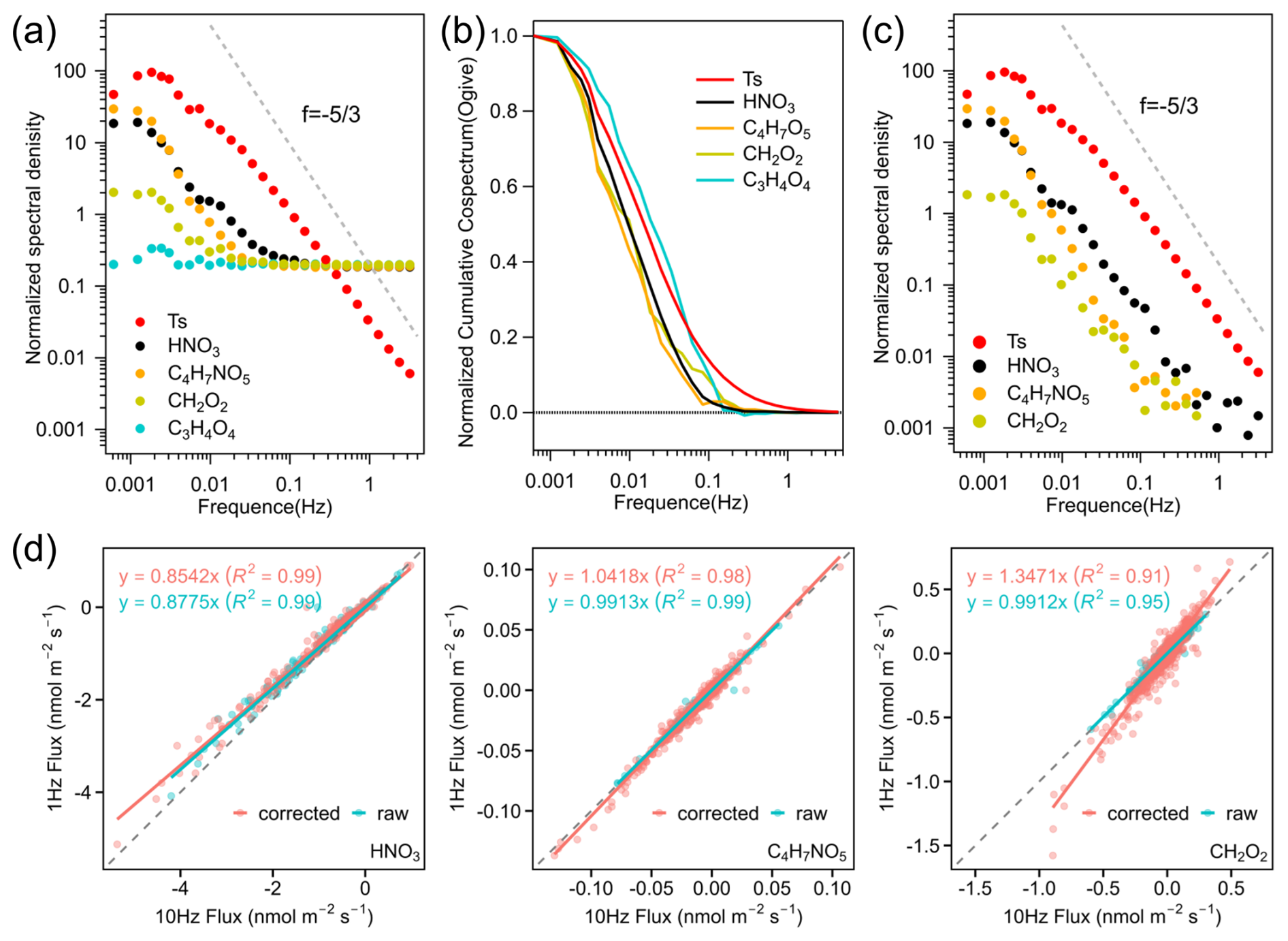
Figure 1 Spectral characteristics of sonic temperature (T_s) and selected species (HNO₃, C₄H₇NO₅, CH₂O₂, C₃H₄O₄) with varying SNRs, for all 30 min intervals (12:00–15:00) during the campaign: (a) mean normalized power spectra; (b) mean normalized cumulative cospectra (ogives) with vertical wind velocity; (c) denoised mean normalized power spectra. Gray dashed lines denote the theoretical Kolmogorov $-\mathrm{5}/\mathrm{3}$ slope. (d) Correlations between 1 and 10 Hz fluxes for HNO₃, C₄H₇NO₅ and CH₂O₂: raw fluxes (blue) and spectrally corrected fluxes (red). The gray dashed line indicating y=x.

Variance-normalized mean power spectral densities (PSDs) for 12:00–15:00 local time show that the T_s spectrum follows the theoretical Kolmogorov $-\mathrm{5}/\mathrm{3}$ slope in the inertial subrange (frequency > 0.002 Hz in this study), confirming adequate sonic anemometer response and well-developed turbulence (Fig. 1a). In contrast, HNO₃ and OOM PSDs deviate significantly from T_s. For species with SNR > 2.2, the spectra flatten above ∼ 0.1 Hz as instrumental white noise becomes dominant. At 10 Hz acquisition, fewer ions are accumulated within each 0.1 s mass spectrum, leading to larger ion-counting fluctuations and increased uncertainty in high-resolution peak fitting, particularly for low-intensity ions. This contributes to enhanced point-to-point fluctuations in the retrieved concentration time series and constitutes an important source of the observed high-frequency instrumental noise. Other instrumental fluctuations, such as detector and ion-source variability, may also contribute. For C₃H₄O₄ (SNR = 2.2), the spectrum is nearly flat across all frequencies with no discernible slope, indicating complete noise domination. This precludes reliable flux characterization, as corroborated by C₃H₄O₄'s near-zero uncorrected raw fluxes (Fig. S8). All OOM species with SNR ≤ 2.2 were therefore excluded from subsequent flux calculations. This spectral screening reduced the number of OOM species retained for flux analysis from 21 to 16.

To assess noise impacts on flux recovery, we further examined normalized cumulative cospectra (ogives) for the selected species (Fig. 1b), which quantify the cumulative flux contribution of turbulent eddies at each frequency. The T_s ogive serves as a near-ideal unattenuated reference and decays smoothly from 1 to 0 across 0.001–2 Hz, confirming the sonic anemometer captures all relevant turbulent scales. For HNO₃ and OOMs, most flux originates from eddies below 0.1 Hz; above 0.1 Hz, ogives fluctuate around zero, indicating random noise dominates and contributes negligibly to net flux. We corrected the power spectra noise before high-frequency loss correction: the high-frequency noise floor was estimated from the flat plateau in HNO₃/OOM power spectra (Fig. 1a), extrapolated to lower frequencies, and subtracted from raw spectra. Noise-corrected spectra (Fig. 1c) exhibit decay behavior similar to T_s, confirming physically realistic turbulent behavior.

In the frequency domain, the measurement system attenuates turbulent fluctuations, causing flux underestimation. Flux loss arises from two sources: (1) low-frequency attenuation due to the 30 min averaging interval and detrending; and (2) high-frequency attenuation from instrument response, path averaging, sensor separation, and inlet tube smearing. High-frequency attenuation is evident in Fig. 1c, where noise-corrected spectra of all species decay steeper than T_s, indicating damping of small-scale eddies.

Low-frequency flux correction was performed using the analytical method of Moncrieff et al. (2004), yielding a single correction factor for all target species per 30 min interval. The mean high-pass spectral correction factor (HPSCF) was 1.13 ± 0.07, corresponding to an average low-frequency flux loss of 11.5 % ± 5.3 % (Text S11).

While the theoretical approach of Moncrieff et al. (1997) can also be used for high-frequency correction, it requires accurate system response time characterization, which is not feasible here due to species-dependent wall adsorption-desorption in the long PFA inlet. High-frequency correction was therefore performed using the empirical field-based method of Ibrom et al. (2007), which compares the unattenuated T_s power spectrum with denoised HNO₃/OOM spectra to yield compound-specific correction factors (Text S12). Mean low-pass spectral correction factors (LPSCF) were 1.12 ± 0.05 for HNO₃, 1.49 ± 0.23 for C₄H₇NO₅, and 1.22 ± 0.11 for CH₂O₂, corresponding to average high-frequency flux losses of 10.9 % ± 3.9 %, 31.5 % ± 9.8 %, and 17.6 % ± 6.6 %, respectively (Table 1).

Table 1 Spectral correction factors, spectral flux losses, mean detection limits (DL), mean sampling random uncertainties, detection rates in all 30 min intervals, and mean daily maximum fluxes for HNO₃ and selected OOMs. Random sampling uncertainty is defined as the mean ${\mathit{\sigma }}_{\mathrm{F}}/F$ for all 30 min fluxes above DL.

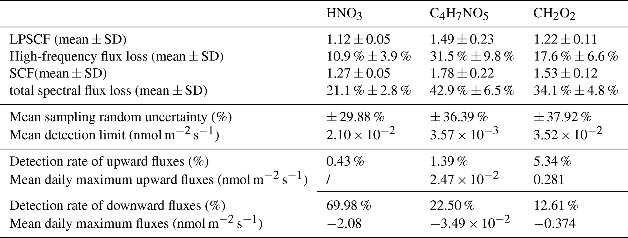
Combining low- and high-frequency corrections yields total spectral correction factors (SCF). For HNO₃, the mean SCF was 1.27 ± 0.05, corresponding to mean total flux loss of 21.1 % ± 2.8 %. Due to species-specific response times and inlet wall interactions, C₄H₇NO₅ and CH₂O₂ exhibited larger SCFs and total flux losses than HNO₃ (Table 1). SCF values for remaining species are listed in Table S1.

3.2 The effects of CIMS mass spectral integration time and ambient water vapor on flux estimates

3.2.1 The effects of mass spectral integration time on flux retrieval

Because the native 10 Hz CIMS measurements contain substantial high-frequency noise, we tested whether increasing the spectral integration time from 0.1 to 1 s could improve flux retrieval. Specifically, every ten consecutive 0.1 s raw mass spectra were co-added to generate 1 s spectra, which were then independently peak-fitted to produce a 1 Hz concentration dataset. Fluxes derived from this independently processed 1 Hz dataset were compared with those obtained from the 10 Hz peak-fitted dataset. The 10 Hz and 1 Hz fluxes, both raw and spectra-corrected, shown in Fig. 1d reveal three key findings: (1) Fluxes from 1 and 10 Hz data are strongly correlated (R²>0.9, p<0.05) for all three species. (2) For HNO₃, 1 Hz raw fluxes are on average 12 % lower than 10 Hz raw fluxes; this difference increases to 15 % after spectral correction, as 1 Hz sampling misses flux contributions from 0.5–5 Hz. (3) For C₄H₇NO₅ and CH₂O₂, raw fluxes differ by < 1 % between 1 and 10 Hz, as their spectra are noise-dominated in the 0.5–5 Hz range with negligible flux contributions. After high-frequency correction, however, 1 Hz corrected fluxes exceed 10 Hz values, driven by larger SCFs for 1 Hz data: 1.78 ± 0.22 (10 Hz) vs. 1.88 ± 0.26 (1 Hz) for C₄H₇NO₅; 1.53 ± 0.12 (10 Hz) vs. 2.09 ± 0.35 (1 Hz) for CH₂O₂. This discrepancy arises from differences in high-frequency noise removal: for 1 Hz data, power spectral density at f>0.2 Hz was treated as noise, while for 10 Hz data the noise floor was determined at f>2 Hz. Overestimation of the high-frequency noise level in 1 Hz spectra leads to an artificially low cutoff frequency (f_c), which in turn produces inflated LPSCFs.

In summary, increasing the spectral integration time improves concentration SNR but introduces systematic flux biases: underestimation for high-SNR species (e.g., HNO₃) and overestimation for medium-SNR species (e.g., C₄H₇NO₅ and CH₂O₂), stemming from errors in noise removal and high-frequency correction. All subsequent analyses therefore used the 10 Hz dataset.

3.2.2 Assessment of Water Vapor Effects

Variations in atmospheric water vapor do not alter the actual flux, but may introduce biases in flux estimates from two sources: (1) distorted quantification of OOM mixing ratios caused by humidity-dependent I-CIMS sensitivity; (2) uncertainties in flux calculation introduced by the use of wet versus dry mole fractions and air density.

We conducted humidity-dependent experiments using surrogate compounds (Text S6). Nitric acid, formic acid, and lactic acid are themselves species for which fluxes were observed in this study. Based on structural similarity, acetic acid was used as a surrogate for monocarboxylic acid other than formic acid, lactic acid for hydroxyl carboxylic acids, pimelic acid for dicarboxylic acids, erythritol for multifunctional alcohols, and 4-nitrophenol for nitrophenol and organonitrate. The experiments showed pronounced compound-dependent humidity effects (Fig. S7): sensitivities of nitric acid, formic acid, lactic acid, and acetic acid decreased with increasing water vapor, whereas those of 4-nitrophenol, pimelic acid, and erythritol increased. For all tested compounds, however, the sensitivities became relatively stable above ∼ 20 mmol mol⁻¹ [H₂O]. During our field campaign, ambient water vapor ranged from approximately 18 to 36 mmol mol⁻¹, with ∼ 98 % of the observations above 20 mmol mol⁻¹. For each surrogate compound, we therefore defined a humidity correction factor (RH_corr) as the ratio of the mean signal response measured at H₂O concentrations above 20 mmol mol⁻¹ to that measured under unhumidified dry-air conditions ([H₂O] = 0.14 mmol mol⁻¹). RH_corr ranges from 0.06 (formic acid) to 0.48 (lactic acid) for water competing compounds and from 1.10 to 1.145 for water stabilizing compounds. The compound-specific RH_corr, or that of the structurally most similar surrogate, was then applied to each target OOM. The surrogate assignments and RH_corr values for all target species are shown in Table S1.

The eddy covariance method quantifies trace gas fluxes arising from the net addition or removal of gases via emission or deposition, rather than from apparent concentration changes induced by water vapor content variations. In this study, the CIMS directly reports wet mole fractions (ppbv) for OOMs and HNO₃, while dry mole fraction is conventionally used in flux calculation. To assess the possible bias associated with using wet mole fraction and wet air density, 1 Hz CIMS inlet air temperature (T_a) and RH were interpolated to 10 Hz to compute water vapor mole fraction using Tetens' equation (Bolton, 1980): $\mathrm{RH}\times \mathrm{6.112}\exp \left(\frac{\mathrm{17.67}{T}_{\mathrm{a}}}{T_{\mathrm{a}}+\mathrm{243.5}}\right)/P$, where P is atmospheric pressure (hPa) measured at the supersite. Fluxes were then recalculated using OOM dry mole fraction and dry air density (dry formulation) after correcting water vapor effect and compared with those using wet mole fraction and wet air density (wet formulation).

The results show that water vapor content is only 0.5 %–2 % by volume. Fluxes from wet and dry formulations agree closely for all species (R²≥0.97, Fig. S7). Wet-formulation fluxes are ∼ 1.1 % higher for HNO₃ (slope = 1.0108), ∼ 1.2 % higher for C₄H₇NO₅ (slope = 1.0122), and ∼ 1.3 % lower for CH₂O₂ (slope = 0.9871). Overall, water vapor-induced bias is within ± 2 % for all species, much smaller than the system's total flux uncertainty (Table 1) and thus negligible. All fluxes reported herein use measured wet mole fraction and wet air density.

3.3 Flux analysis

After the above SNR and spectral screening, we observed 16 OOM species (including 12 CHO-OOMs and 4 CHON-OOMs) with detectable fluxes during the summer campaign. Time series of concentrations and fluxes of the 4 selected species (HNO₃, C₄H₇NO₅, CH₂O₂, and C₃H₄O₄) are provided in Fig. S6. Daily maximum mixing ratios of the medium-SNR OOMs C₄H₇NO₅ and CH₂O₂were 0.149 ± 0.021 and 1.146 ± 0.166 ppbv, respectively. Their downward flux detection rates (the fractions of flux estimates exceeding their respective detection limits) are 22.5 % and 12.6 % of all 30 min intervals, with corresponding mean daily maximum downward fluxes of $-\mathrm{3.49}\times {\mathrm{10}}^{-\mathrm{2}}$ and −0.374 nmol m⁻² s⁻¹ (Table 1). Their upward flux detection rates were lower, ranging from 1.4 % to 5.3 % of all 30 min intervals.

The OOM fluxes observed at this urban site were generally lower than those reported above forest canopies, although the differences were typically within one order of magnitude (Fulgham et al., 2019; Nguyen et al., 2015; Vermeuel et al., 2023). For example, formic acid maximum fluxes above forests were around 1–2 nmol m⁻² s⁻¹, either emission or deposition, with mean maximum mixing ratio around 2.5 ppbv. Mean daily maximum fluxes of total 85 OOMs detected by I-CIMS were around 2.5 nmol carbon m⁻² s⁻¹ for both emission and deposition over a coniferous forest (Vermeuel et al., 2023), compared with summed downward and upward fluxes of 0.60 and 0.34 nmol carbon m⁻² s⁻¹, respectively, for the 16 OOM species measured in our study.

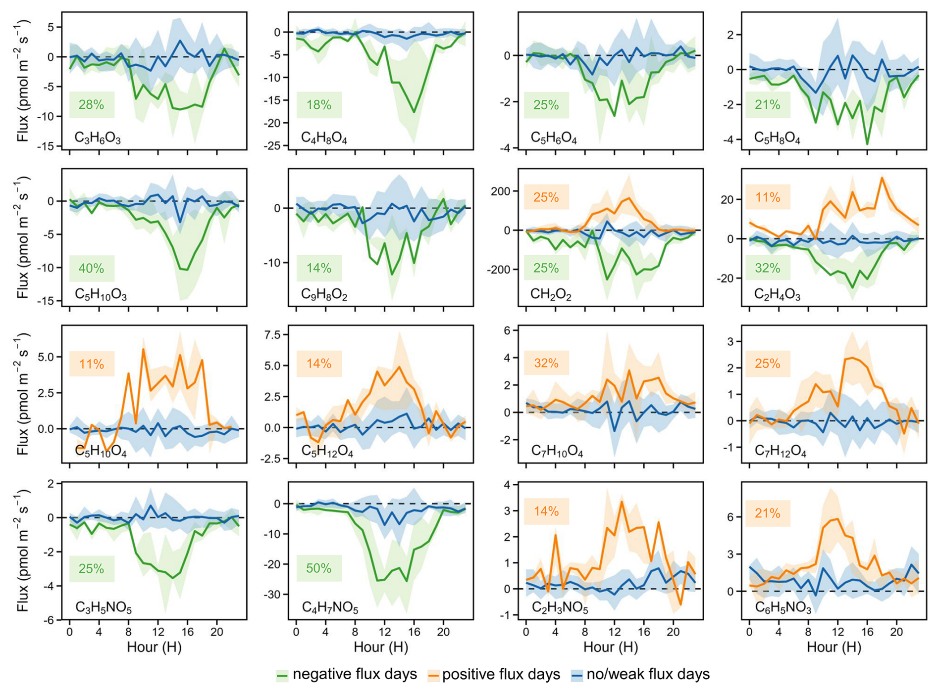
Figure 2 Diurnal cycles of OOM fluxes, grouped by flux sign: positive (orange), negative (green), and no/weak flux (blue) days. Percentages denote the fractions of positive and negative flux days relative to all observation days; shaded areas mark 25th–75th percentiles.

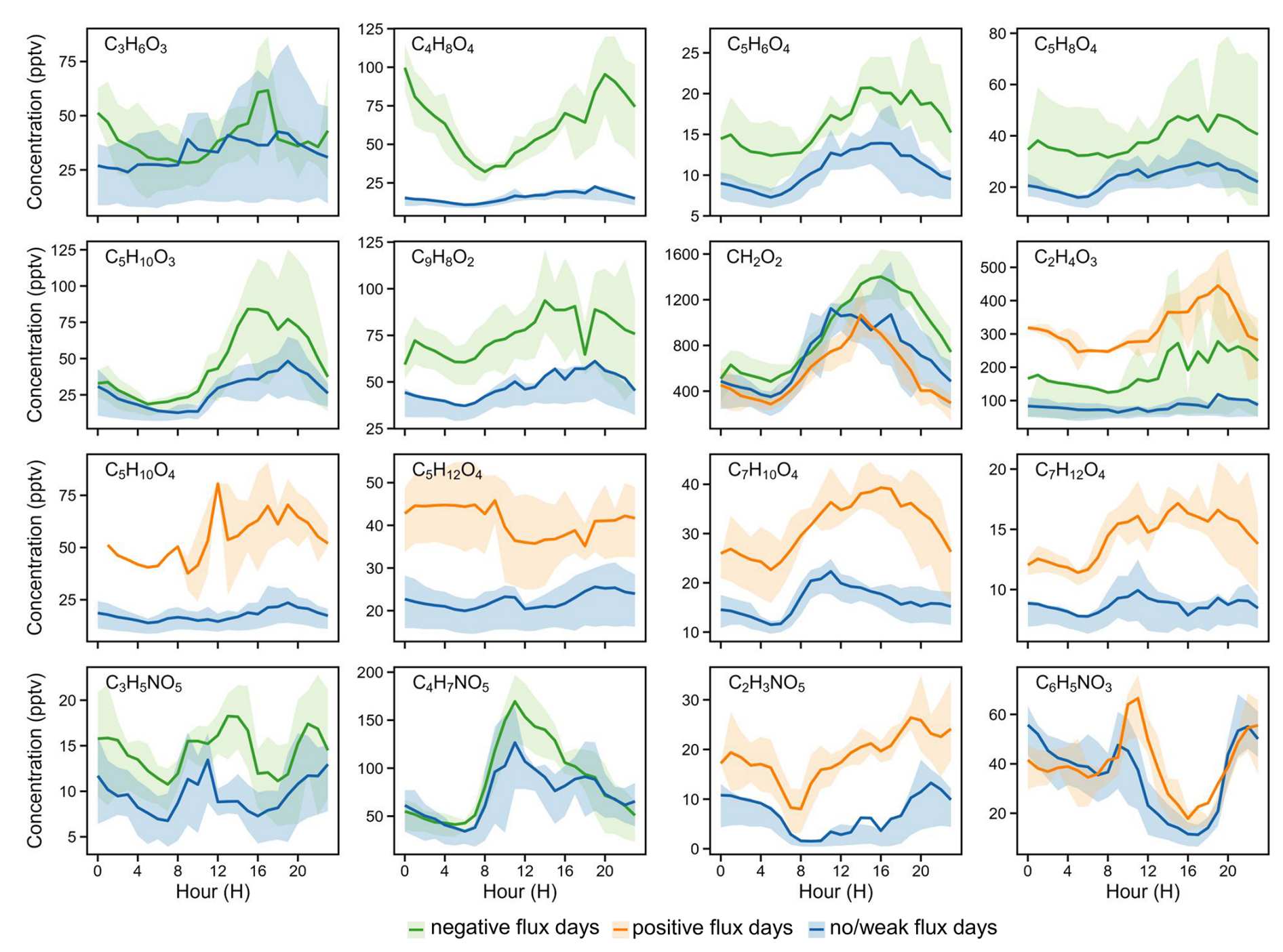
Figure 3 Diurnal cycles of OOMs mixing ratios grouped by flux sign: positive (orange), negative (green), and no/weak flux (blue) days. Shaded areas represent the corresponding 25th and 75th percentiles.

Based on the direction and magnitude of fluxes, observation days were classified into three categories: positive-flux days, negative-flux days, and no/weak-flux days. Mean diurnal variations of fluxes on these three categories of days are presented in Fig. 2 for the 16 OOM species. Below we examine OOM flux directions, magnitudes, and their dependences on mixing ratios (Fig. 3) and key meteorological parameters (u^*, $z/L$, temperature, solar radiation, and wind direction; Figs. S10–S14).

The possible dependence of the observed fluxes on wind direction was examined by comparing horizontal wind-vector distributions among positive, negative, and no/weak flux conditions (Fig. S14). The three flux categories showed substantial overlap in wind-vector space, and no directional preference was observed for HNO₃ or the 16 OOM species. Moreover, because the campaign covered only 28 valid days, the directional sampling was uneven and does not allow robust wind-direction-resolved attribution.

3.3.1 CHO-OOMs

Based on flux directions (Fig. 2), the 12 CHO-OOMs are classified into three groups: deposition-dominated, emission-dominated, and bidirectional OOM, indicating complex source-sink dynamics over urban surfaces. Six deposition-dominated OOMs (C₃H₆O₃, C₄H₈O₄, C₅H₆O₄, C₅H₈O₄, C₅H₁₀O₃, C₉H₈O₂) showed negative fluxes on 14 %–40 % of observation days, with mean daily maximum values of −8.86, −17.68, −2.61, −4.26, −10.37, and −12.60 pmol m⁻² s⁻¹, respectively. This indicates deposition exceeded near-surface emissions and chemical production on these days, making urban surfaces a net sink for these species.

Mixing ratios of these six species were significantly higher on negative-flux days than on no/weak-flux days (Fig. 3). Elevated concentrations appearing to be the direct driver of the observed negative fluxes. No statistically significant differences in key turbulence parameters (u^*, $z/L$) were observed between the two categories of days (Figs. S10 and S11). However, deposition flux diurnal variations were modulated by turbulence: maximum fluxes for all six OOMs consistently occurred between 12:00–16:00 when turbulence was most fully developed, rather than peak concentration hours. As widely documented in previous I-CIMS studies, these species are inferred to be isoprene oxidation products (2-methylglyceric acid C₄H₈O₄; IEPOX+ISOPOOH C₅H₁₀O₃), glutaric acid C₅H₈O₄and lactic acid C₃H₆O₃ formed from oxidation of anthropogenic and biogenic precursors, citraconic acid C₅H₆O₄ and trans-cinnamic acid C₉H₈O₂ from biomass burning (Oghama et al., 2025).

The second group, comprising C₅H₁₀O₄, C₅H₁₂O₄, C₇H₁₀O₄, and C₇H₁₂O₄, exhibited positive fluxes on 11 %–32 % of observation days, with mean daily maximum values of 5.35, 4.90, 3.08, and 2.37 pmol m⁻² s⁻¹, respectively. On positive-flux days, these species showed enhanced daytime emissions and elevated concentrations, coinciding with higher temperature and solar radiation than no/weak-flux days (Figs. S12 and S13). These OOMs likely originate from direct surface emissions or form via rapid near-surface photooxidation of precursors. The resulting upward concentration gradient gives rise to the observed apparent positive fluxes. C₅H₁₂O₄ is 2-methyltetrols from isoprene oxidation. C₅H₁₀O₄ is an isoprene oxidation product (potentially a hydroxy-hydroperoxy carbonyl, Ramírez-Romero et al., 2026) but also found in food cooking emission (Reyes-Villegas et al., 2018; Mehra et al., 2021). Saturated dicarboxylic acid C₇H₁₂O₄ may be from thermally enhanced vegetation emission or biomass burning (Kawamura and Bikkina, 2016). C₇H₁₀O₄ is possibly a toluene-derived peroxide-bicyclic alcohol (Wang et al., 2020).

The third group, comprising CH₂O₂ (formic acid) and C₂H₄O₃ (peracetic acid), exhibited bidirectional flux patterns. Formic acid and peracetic acid have various primary emission sources and secondary photochemical origins, so their bidirectional fluxes reflect competition between atmospheric deposition and near-surface emissions plus chemical production. In fact, no/weak-flux days accounted for 50 % and 57 % of the observation days for the two OOMs. We attribute these weak/undetectable net fluxes to the cancellation of emission and deposition fluxes, rather than an absence of surface exchange processes.

3.3.2 CHON-OOMs

CHON-OOMs comprised two acyl peroxy nitrates (PAN: C₂H₃NO₅; PPN: C₃H₅NO₅), one isoprene-derived organonitrate (C₄H₇NO₅), and one nitrophenol (C₆H₅NO₃). Both acyl peroxy nitrates form from acyl peroxy radicals + NO₂: PAN from anthropogenic or biogenic VOC oxidation, PPN from anthropogenic n-alkanes (Min et al., 2012; Phillips et al., 2013; Turnipseed et al., 2006; Wolfe et al., 2009). C₄H₇NO₅, often assigned to methacrolein and methyl vinyl ketone hydroxy nitrate (MACN/MVKN), are multi-generational oxidation products of isoprene in NO_x-influenced regions (Mayhew et al., 2022; Tsiligiannis et al., 2022). Nitrophenol (C₆H₅NO₃) is anthropogenic, originating from primary combustion/industrial emissions and secondary oxidation of phenolics with NO_x.

Positive fluxes of PAN and nitrophenol were detected on 14 % and 21 % of the observation days, with corresponding daily maximum flux of 3.35 and 5.86 pmol m⁻² s⁻¹, respectively; higher mean radiation was observed on these positive-flux days (Fig. S13). Negative fluxes of PPN and MACN/MVKN were observed on 25 % and 50 % of the observation days, with their daily maximum flux on negative-flux days reaching −3.56 and −25.74 pmol m⁻² s⁻¹, respectively. Although the four species exhibited unimodal or bimodal concentration patterns (Fig. 3), their flux maxima all occurred during the daytime with fully developed turbulence.

3.3.3 Summer campaign-averaged OOMs fluxes and comparison with HNO₃

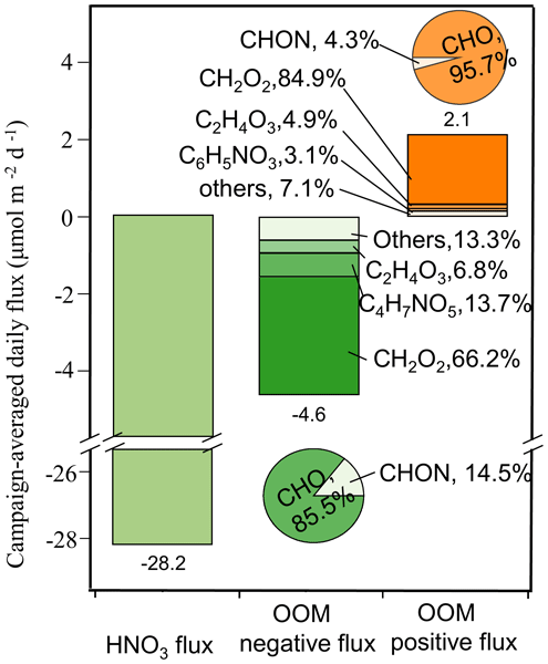
Given the complex flux behavior of OOMs, we aggregated all positive and negative fluxes separately for the entire summer campaign and calculated campaign-averaged daily values for each species (Fig. 4a). Campaign-averaged daily negative flux of the 16 OOM species was 4.6 µmol m⁻² d⁻¹, with CHON-OOMs contributing 85.5 % and CHO-OOMs contributing the remaining 14.5 %. The top three contributors to the total negative flux were the formic acid, isoprene-derived MACN/MVKN (C₄H₇NO₅), and peracetic acid, collectively accounting for 86.7 % of the total OOM negative flux. Total campaign-averaged daily positive flux of OOMs was 2.1 µmol m⁻² d⁻¹, equal to 46 % of the total negative flux. The positive flux was dominated by formic acid, accounting for 84.9 % of the total OOM positive flux.

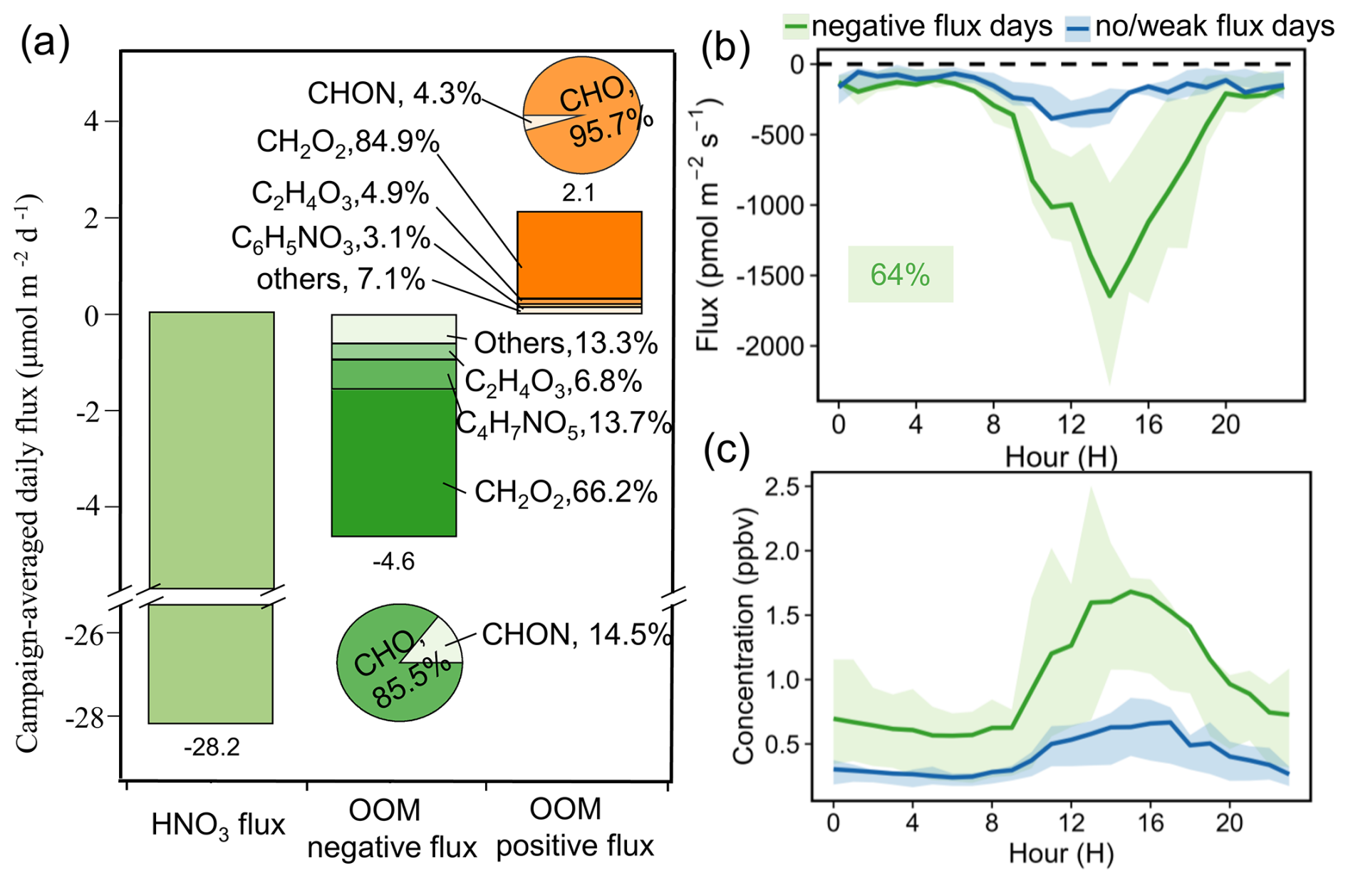
Figure 4 (a) Campaign-averaged daily fluxes (including species contributions). Diurnal cycles of HNO₃: (b) fluxes and (c) mixing ratios, grouped by flux sign: negative (green), and no/weak flux days (blue). Percentages denote the fractions of negative flux days relative to all observation days. Shaded areas represent the corresponding 25th and 75th percentiles.

For comparison, total campaign-averaged daily negative flux of all OOMs accounted for only 16.3 % of that of nitric acid, which showed downward flux in 70.0 % of all 30 min intervals (Table 1) and in 18 of 28 observation days (Fig. S6). As a deposition-dominated species, HNO₃ mean diurnal flux on negative-flux days was unimodal, peaking at −1.65 nmol m⁻² s⁻¹ at 14:00 local time (Fig. 4b). This HNO₃ peak was one to three orders of magnitude larger than the individual OOM flux peaks on negative-flux days, but was closer to mean HNO₃ peak fluxes of −2.636 and −0.558 nmol m⁻² s⁻¹ reported over forest canopies (Horii et al., 2006; Nguyen et al., 2015). In terms of mixing ratio, mean daily maximum of HNO₃ (1.16±0.74 ppbv) was one to two order of magnitude higher than the OOMs (tens or hundreds of pptv, Fig. 3).

4 Conclusion

This is the first direct eddy covariance flux measurement of pptv-level OOMs in an urban environment. We optimized the flux processing workflow for low-SNR OOMs, including noise subtraction from power spectra, compound-specific spectral correction using the empirical Ibrom method, and uniform lag time determination using high-SNR HNO₃ as a reference tracer. We also systematically investigated the effects of mass spectral integration time and water vapor on flux estimates.

While urban environments are generally recognized as having more severe anthropogenic organic pollution, the OOM fluxes measured at this urban site were generally lower than those reported above forest canopies, although the differences were typically within one order of magnitude. For example, the maximum formic acid flux in our study was approximately 3–5 times lower than values reported above forests. The summed downward or upward fluxes of the 16 OOMs measured here were also lower than the total flux of 85 OOMs detected by I-CIMS over a coniferous forest (Vermeuel et al., 2023), although these totals are not directly comparable because of the different numbers and identities of OOM species included. These differences may partly reflect the contrasting source environments: forest-canopy flux measurements were conducted only a few meters above strong biogenic emission sources, whereas our study was conducted at a suburban university campus distant from downtown areas, industrial zones, and major traffic emission sources.

Our flux observation of HNO₃ and 16 OOM species reveals complex bidirectional exchange shaped by competing biogenic/anthropogenic emissions, near-surface photochemistry, and dry deposition. The campaign-averaged total daily OOM deposition flux (4.6 µmol m⁻² d⁻¹) was four times larger than the total daily emission flux (2.1 µmol m⁻² d⁻¹). Isoprene-derived organonitrate C₄H₇NO₅, IEPOX+ISOPOOH (C₅H₁₀O₃), formic acid (CH₂O₂), and nitrophenol C₆H₅NO₃ were identified as the dominant contributors to the total OOM fluxes.

Several limitations of the present study should be noted. First, the relatively short campaign limits the representation of seasonal variability, atmospheric circulation regimes, and specific synoptic events. Second, observations from a single urban site cannot represent the diversity of urban surface characteristics and atmospheric environments. Third, the indirect sensitivity calibration for compounds lacking authentic standards introduces larger concentration and flux uncertainties than compound-specific calibration. Finally, iodide-adduct I-CIMS selectively detects OOMs with favorable iodide-clustering efficiencies, and therefore does not capture the entire atmospheric OOM pool. Year-round measurements are ongoing and will enable systematic assessment of the seasonal evolution of OOM fluxes and their dependence on meteorological, chemical, and circulation conditions. Multi-site measurements, together with complementary chemical-ionization techniques, will be needed to better characterize the seasonal, chemical, and spatial variability of OOM surface–atmosphere exchange.

Nevertheless, this work establishes the foundation for future study and underscores the necessity of combining flux observations with advanced modeling to fully elucidate the source and sink of OOMs in urban atmosphere. The results offer essential observational constraints for chemical transport models, which currently lack accurate parameterizations for OOM dry deposition due to limited field measurements.