Evidence for the impact of fire activity on daily variations of IASI mid-tropospheric CO₂ anomalies at 8–11 km over South America: a pyroconvective fingerprint

Biomass burning is a major, highly variable source of atmospheric CO₂, but its impact on the free troposphere remains difficult to quantify because of uncertainties in injection heights and transport. In the tropics, intense fires can trigger pyroconvective plumes that loft combustion products to the mid- and upper troposphere. However, most fire emission inventories and global CO₂ inversions still assume simplified vertical distributions of CO₂ emitted by fires. Weighted columns of CO₂ retrieved from remote sensing instruments that are sensitive to such high-altitude enhancements can inform of such dynamics. Here we combine mid-tropospheric CO₂ (MT-CO₂) retrievals from three IASI instruments with GOES-16 observations of Fire Radiative Energy (FRE) to link daily MT-CO₂ anomalies observed by IASI at 8–11 km altitude to South American fire activity during the 2020 burning season, while accounting for long-range horizontal transport of anomalies. From August–October 2020, about 66 % of the detected anomalies originate from long-range or unknown sources and are discarded. For the remaining anomalies attributed to local fires, 72 h back trajectories do intersect with at least one active fire detection for 75 % of them. Their daily sum co-varies strongly with FRE, with the ratio between the two depending on the dominant horizontal transport regime. A comparison with the CAMS inversion-optimised CO₂ product (v23r1), sampled with the IASI vertical weighting, shows that the model fails to reproduce both the amplitude and structure of the observed anomalies. Overall, our results demonstrate that IASI MT-CO₂ anomalies carry an observational fingerprint of tropical fire activity.

1 Introduction

A comprehensive understanding of the global carbon cycle, including its sources and sinks, is essential for predicting future climate variations (Friedlingstein et al., 2025; Intergovernmental Panel On Climate Change (IPCC), 2023). In the carbon cycle, open biomass burning is a major, rapidly varying source of atmospheric trace gases, including mostly carbon dioxide (CO₂), which represents about 90 % of the emissions, and carbon monoxide (CO) for about 6 % and methane (CH₄) for about 1 % (Andreae, 2019). Long-term inventories report gross carbon emissions from fires of about 2.1–2.2 Pg C yr⁻¹ for 1997–2016, with pronounced interannual peaks (e.g., ∼ 3.0 Pg C in 1997 during El Niño; (van Der Werf et al., 2017)). The 2024 State of Wildfire report (Jones et al., 2024) indicates that for March 2023–February 2024, fire emissions approached ∼ 2.4 Pg C while 2024 global fossil-fuel CO₂ emissions are ∼ 10 Pg C yr⁻¹. Thus, the gross fire flux is about 20 % of annual fossil emissions, although the net atmospheric impact depends on post-fire regrowth versus permanent land-use change (Friedlingstein et al., 2025). Moreover, about 84 % of global fire carbon emissions originate in the tropics (23.5° N–23.5° S), ∼ 1.83 Pg C yr⁻¹ out of a 1997–2016 mean of ∼ 2.16–2.20 Pg C yr⁻¹ (van Der Werf et al., 2017). Within the tropics, contributions are strongly skewed toward Africa (roughly 50 % in long-term estimates), followed by South America (20 %) and tropical Asia (10 %). These characteristics make fires, and especially tropical fires, a dominant driver of interannual variability in atmospheric CO₂ growth rates and a critical process to monitor (Langenfelds et al., 2002). Fire emission inventories rely on satellite observations of burned areas and Fire Radiative Power (FRP, MW) to infer carbon fluxes via assumed fuel loads, combustion completeness, and biome-specific emission factors. However, these estimates carry substantial uncertainties, first on the quantification of the emissions (Liu et al., 2020) but also on the estimation of the plume injection height and subsequent transport (Whaley et al., 2025).

Indeed, most of this carbon is released and mixed within the planetary boundary layer, but a fraction is lofted into the free troposphere by fire-induced convection (pyroconvection), where it is transported over long distances and influences the mid- and upper-tropospheric composition. This lofted fraction is modest in the mean, of the order of 5 % of daytime plumes globally (Rio et al., 2010) and 3 %–20 % over the Amazon (Gonzalez-Alonso et al., 2019), but it is dominated by the most intense fires and can rise sharply during peak events and toward the end of the burning season. Crucially, the vertical distribution of fire emissions is among the least constrained aspects of the biomass-burning budget: global CO₂ inversions have long relied on prescribed or parameterized injection profiles rather than observations, so errors in injection height propagate directly into inferred surface fluxes and into the simulated free-tropospheric carbon field.

Direct observations of the atmospheric CO₂ distribution are so needed to evaluate inventory biases, quantify the net impact of fires on the concentration field and understand the injection heights in the atmosphere. In this context, satellites play a central role in observing atmospheric CO₂ at the global scale and in identifying source regions and processes. Beyond global coverage, spaceborne retrievals are sensitive to different parts of the atmospheric column: while a single partial column does not resolve a full vertical profile, it isolates the contribution of a specific layer (here the mid-troposphere), and combining columns with differing vertical sensitivities further constrains the vertical distribution of CO₂: depending on instrument and spectral band, they deliver total columns (XCO₂) or partial columns targeted to specific layers. In particular, infrared (IR) sounders retrieve mid-tropospheric (MT) CO₂ partial columns (Crevoisier, 2018; Crevoisier et al., 2009) that have been used to study fire-related signals. Early work using NOAA's TIROS Operational Vertical Sounder (TOVS) revealed a robust diurnal signature over fire regions, formalized as the evening-minus-morning MT-CO₂ difference (the Daily Tropospheric Excess, denoted DTE), associated with uplift reaching up to 200 hPa (Chedin et al., 2008; Chédin et al., 2005). This signal has been interpreted as the consequence of pyroconvection uplifting combustion products into the mid- and upper troposphere, together with horizontal transport and the strong diurnal cycle of fire activity (Fromm et al., 2019; Peterson et al., 2022; Tang et al., 2022). Afterwards, (Thonat et al., 2015) further showed that the morning–evening CO difference, using observations from IR sounders Atmospheric Infrared Sounder (AIRS) and Infrared Atmospheric Sounding Interferometer (IASI), correlates strongly with independent active-fire observations and emissions. Beyond these diurnal-difference approaches, a substantial body of work has used satellite observations to track fire-emitted gas, but mostly using CO observations. Indeed, fire-driven CO enhancements often exceed the background by more than 100 %, yielding a clear atmospheric signal (e.g., Thonat et al., 2015). By assimilating Measurement of Pollution in the Troposphere (MOPITT), AIRS, IASI, and more recently Tropospheric Monitoring Instrument (TROPOMI) CO into chemical transport models, several studies have quantitatively attributed observed CO enhancements to biomass-burning sources at global and regional scales, including the Amazon and other tropical basins (e.g. Naus et al., 2022; Nechita-Banda et al., 2018). This top-down approach demonstrates that, once transport and chemistry are explicitly represented, the atmospheric composition signal can constrain fire emissions and their variability.

In contrast to CO, a central challenge for CO₂ observations is the inherent weakness of the fire-driven CO₂ signal relative to the background, which translates into a lower signal to noise than for CO. As a result, a direct anomaly-based attribution of mid-tropospheric CO₂ to daily fire activity, by tracking CO₂ fire-driven anomalies themselves while explicitly accounting for transport, has not yet been established.

Here, we address this gap by using mid-tropospheric CO₂ retrievals from three IASI instruments to quantify CO₂ anomalies and relate them to South American fire activity from Geostationary Operational Environmental Satellite (GOES-16) and associated emissions, while explicitly accounting for horizontal transport. We focus on the 2020 fire season (i.e. August to October), marked by severe events in the southern Amazon, Northern Argentina and Pantanal (the world's largest tropical wetland, spanning Brazil, Bolivia and Paraguay). Section 2 describes the satellite data analyzed to conduct the study and Sect. 3 the methodology developed to include horizontal transport, illustrated by case studies. Section 4 analyzes the relationship between fire activity and mid-tropospheric CO₂ while taking into account different transport regimes. Section 5 discusses the results and Sect. 6 gives the conclusion.

2 Satellite data

2.1 Mid-Tropospheric CO₂ anomalies from IASI observations

Mid-Tropospheric CO₂ columns are retrieved from the three IASI instruments flying onboard the European Metop platforms, Metop-A (2007–2020), Metop-B (2013–2020), and Metop-C (2019–present) (Crevoisier et al., 2009). Figure 1 summarizes the IASI CO₂ vertical sensitivity, expressed in pressure, for 5° latitude bands centered from 32.5° S to 32.5° N. The peak sensitivity of the retrievals lies between about 360 and 235 hPa, corresponding in a tropical atmosphere to roughly 8–11 km above sea level. The central 50 % of the contribution generally comes from layers between 5 and 12 km, while sensitivity is very low below 4 km and above 14 km. Consequently, IASI mainly observes, on top of the large-scale background, CO₂ emissions that have been transported to those high altitudes, and in particular those associated with pyroconvection, as discussed by Chedin et al. (2008). These retrievals are assimilated with ECMWF C-IFS system to provide CAMS CO₂ forecasts and reanalysis (Agustí-Panareda et al., 2023). CO₂ retrievals are available over the tropical region between 35° S and 35° N, twice a day, at 09:30 a.m. and 09:30 p.m. Local Time at the Equator. The uncertainty attached to a single retrieved mid-tropospheric column is estimated around 1 ppm (Crevoisier, 2024). Since clouds have a strong impact on radiances measured in the thermal infrared, only clear-sky situations are considered. To further limit residual cloud contamination stemming from potential undetected clouds by the filtering described in Capelle et al. (2018), Crevoisier et al. (2009), we also consider the collocated AVHRR cloud fraction, provided in the L2 IASI data from EUMETSAT and retain only observations where corresponding cloud fraction is below 20 %. As a thermal-infrared sounder, IASI is in principle sensitive to aerosols; however, we use clear-sky scenes only, strongly absorbing aerosols such as desert dust are screened within the same retrieval framework as the IASI dust product (Capelle et al., 2018), so any residual aerosol effect cannot plausibly generate the spatially coherent.

Given that CO₂ is well mixed in the atmosphere, source-driven variations of its atmospheric mixing ratio are small relative to the background. Therefore, the CO₂ concentration analysis is conducted in terms of anomaly instead of absolute concentration itself. Since CO₂ concentration background varies with latitude and time, we define a dynamic background, estimated for each IASI observation by selecting every CO₂ observations lying within a ±3 d window, ±2° latitude band (bands from 35° S to 35° N, ocean and land indistinctly) and for longitudes between 180° W to 180° E. This background is calculated for the morning and the evening overpasses separately. To mitigate the overrepresentation of high fire-season values in the background computation, outliers are removed using the interquartile-range (IQR) filter: using the first (Q1) and third (Q3) quartiles, we define IQR = Q3–Q1 and discard observations lying outside the interval Q1–1.5 × IQR, Q3+1.5 × IQR. Then, the median of the filtered set is taken as the background. Figure 2 shows the monthly distribution of IASI MT-CO₂ for the months from August to October over South America in 2020, together with the derived CO₂ anomalies. Signatures of biomass burning regions are well seen over land but also over ocean, and especially over the Atlantic Ocean. The latitudinal variation of MT-CO₂, which increases with latitude, is no longer seen in the anomaly. The MT-CO₂ anomaly follows the expected seasonal variation of biomass burning regions: In August, positive anomalies are still moderate and relatively patchy, with enhancements mainly over central–southern Amazonia and along the southern edge of the basin, while most of the continent exhibits near-zero or slightly negative anomalies. In September, the positive anomaly pattern intensifies and expands, forming a broad band over southern Amazonia that extends toward Cerrado and Pantanal and is accompanied by enhanced anomalies over the adjacent tropical Atlantic, indicative of export of polluted air masses. October displays the largest positive anomalies, with a marked maximum over central–southern Amazonia and persistent enhancements over the Pantanal and downwind Atlantic. Overall, the timing and location of these positive MT-CO₂ anomalies qualitatively follow the seasonal evolution of fire activity inferred from the mean daily FRE fields derived from GOES-16 (Fig. 3), with stronger and more extensive anomalies occurring over and downwind of regions with intense burning.

We have chosen to focus this study on the year 2020 because the three IASI instruments were flying simultaneously, increasing the number of observations for the same area. To minimize inter sensor offsets, anomalies are computed separately for each IASI instrument before aggregation. We then average anomalies onto 0.5° daily grids for the morning and evening overpasses and retain grid cells with at least two contributing observations to increase reliability. In the following, we analyze only anomalies that exceed the natural variability of the background. Based on sensitivity tests that balance sample size against false detections, we adopt a threshold of 4 ppm to select anomalies representing the excess of CO₂ from the background in the altitude range of 8 to 11 km. Because a CO₂ enhancement confined below ≈ 4 km cannot produce a mid-tropospheric anomaly of this magnitude in the IASI retrieval (a uniform +20 ppm filling the 0–4 km boundary layer yields a retrieved signal of only ∼ 1.5 ppm), this threshold selects, by construction, emissions that have been lofted into the free troposphere by convective or pyroconvective transport.

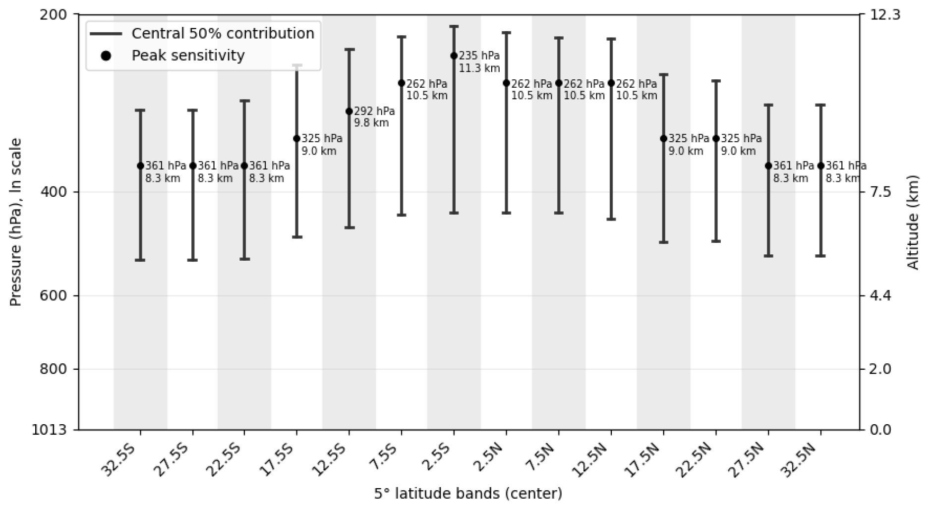
Figure 1 IASI MT-CO₂ vertical sensitivity expressed as pressure and altitude for 5° latitude bands (centered from 32.5° S to 32.5° N). For each band, the vertical black line with end caps shows the central 50 % of the column that contributes most to the IASI CO₂ retrieval (from the 25th to the 75th percentile of the weighting-function contribution). The black dot marks the pressure of maximum sensitivity (“peak sensitivity”), and the annotation gives both the peak pressure (hPa) and its approximate tropical altitude (km) derived from a simple hydrostatic tropical profile.

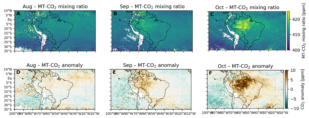
Figure 2 Top row: Monthly IASI mid-tropospheric CO₂ over tropical South America during the 2020 fire season (both overpasses) for August, September, and October 2020. Bottom row: corresponding to monthly mean IASI MT-CO₂ anomalies (i.e. departures from a latitude- and time-dependent background).

2.2 Fire Radiative Power from GOES-16

In this study, fire activity is characterized using the GOES-16 (GOES-East) FRP-PIXEL product. This dataset is generated using the Geostationary Fire Thermal Anomaly (FTA) algorithm and provides landscape-level Fire Radiative Power (FRP) at full spatio-temporal resolution (Xu et al., 2010, 2017, 2021). FRP is expressed in megawatts (MW) and represents the thermal energy emitted by an active fire at the time of satellite observation. It is directly related to the rate of fuel consumption and to the emission rate of smoke and various chemical species (Roberts et al., 2005). The FTA algorithm applied to GOES-16 ABI estimates FRP using the mid-infrared (MIR) radiance method, based on measurements in the 3.9 µm spectral band. This method accounts for the radiative properties of both the fire pixel and its surrounding background.

Compared to polar-orbiting sensors such as MODIS (aboard Terra and Aqua) and VIIRS (aboard Suomi NPP and NOAA-20), the GOES-16 ABI FRP-PIXEL product offers a major advantage in temporal resolution. While polar orbital satellites instruments such as MODIS and VIIRS typically provide two observations per day at a given location, GOES-16 ABI offers sub-hourly observations at a 15 min interval. This high temporal resolution is critical for capturing the full diurnal cycle of fire activity (Andela et al., 2015), which can vary significantly throughout the day. Indeed, the hour of peak fire activity depends on the type of fire, vegetation and atmospheric conditions (Giglio, 2007; Giglio et al., 2018; Li et al., 2019; Tang et al., 2022) and is therefore linked to the biome where the fires occur.

The GOES-16 FRP-PIXEL product provides FRP values at 2 km spatial resolution from 2018 to the present, enabling near-continuous monitoring of fire dynamics across the Americas. We select high-confidence fire detections (confidence ≥ 70 %) with FRP > 100 MW to limit false detections after sensibility tests. We then compute Fire Radiative Energy (FRE) which is the time-integral of FRP, i.e. the cumulative thermal energy released by burning because it scales with biomass consumed and thus with emissions (Wooster et al., 2005). We compute FRE from GOES-16 FRP by first aligning all detections to fixed 15 min UTC slots (instrument cadence) and assuming FRP is piecewise constant over each slot; the energy of a slot is:

$$\begin{array}{}\text{(1)}& {\mathrm{FRE}}_{\mathrm{slot}}=\sum \mathrm{FRP}\cdot \mathrm{\Delta }t\end{array}$$

where Δt=900 s. For emission fields, we assign slot energies to 0.5° cells, sum to daily FRE, and average over calendar days to yield mean daily FRE (GJ d⁻¹). Figure 3 shows maps of means daily FRE for each month (from August to October) along with the geographical context of the main regions we rely on: the northern Amazonia region is derived from Ecoregions 2017 definition (https://ecoregions.appspot.com/, last access: 13 September 2026); the Cerrado and Pantanal regions are taken from the Global Forest Watch (https://www.globalforestwatch.org/, last access: 13 September 2026) biome boundaries for Brazil; and the South Amazonia deforestation front is extracted from the WWF Deforestation Fronts 2020 (https://globil.panda.org/datasets/panda::deforestation-fronts-2020-1/about, last access: 13 September 2026) dataset. The spatial distribution of mean daily FRE (Fig. 3) shows clear location-linked contrasts during the 2020 South American fire season. In August, high values cluster over central–southern Amazonia, the Pantanal, and northern Argentina–Uruguay. In the southern Brazilian Amazon, 2020 saw heightened use of deforestation and understory fires relative to 2019, consistent with the strong FRE detected along the “Arc of Deforestation” (Silveira et al., 2022). The Pantanal signal reflects exceptional dryness and record burned extent in 2020, which primed wetlands and adjacent savannas for large, intense fires (Garcia et al., 2021). In northern Argentina–Uruguay, FRE aligns with fire-prone grassland systems where burns are commonly used within pasture and rangeland management (Cuello et al., 2020). In September, activity intensifies and expands. Elevated FRE spreads across central–southern Amazonia toward the Cerrado boundary, part of the long-recognized deforestation corridor, and increases within the southern Cerrado, which typically peaks late in the dry season (Nogueira et al., 2007). The Pantanal reaches its seasonal maximum under continuing drought stress and extensive fuel availability (Garcia et al., 2021). By October, the area of highest FRE contracts, especially in southern Amazonia, while elevated values persist in parts of the Cerrado, Pantanal, and northern Argentina–Uruguay, consistent with late dry-season burning in savanna and grassland biomes and the hydrological deficit in the Pantanal.

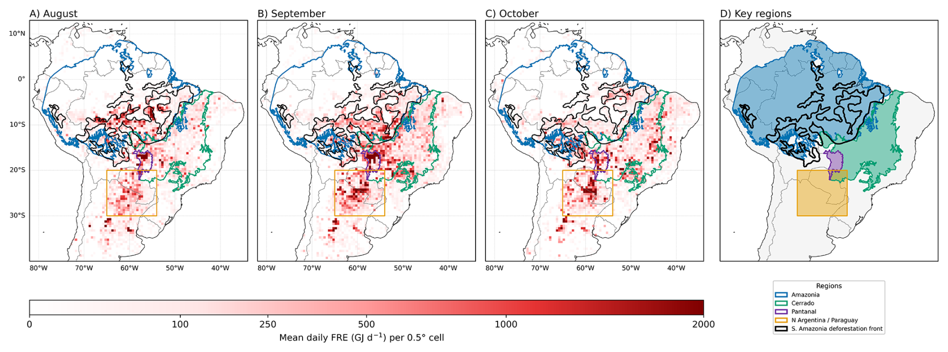
Figure 3 Monthly mean daily Fire Radiative Energy (FRE) over South America on a 0.5° grid. Panels (A)–(C) show August, September, and October 2020, respectively. The colour scale gives mean daily FRE in GJ d⁻¹ per 0.5° cell, ranging from white (no detected FRE) to dark red (high FRE). Panel (D) shows the geographical context of main regions. The outlines of these regions, together with the South Amazonia deforestation front, are also overlaid on Panels (A)–(C).

3 Analysis of mid-tropospheric CO₂ anomalies

3.1 Description of the method

To remove the anomalies stemming from long-range transport and keep only the anomalies that can be attributed to local sources, we use the Lagrangian transport model LAGRANTO (Sprenger and Wernli, 2015), which allows tracking the history of CO₂ anomalies. LAGRANTO computes air parcel trajectories from three-dimensional wind fields and is widely used for source–receptor analyses in atmospheric science. From each anomaly we run 72 h backward trajectories initialized at 250 hPa, the averaged peak of sensitivity of IASI for the considered latitudes (Fig. 1), using ERA5 reanalysis winds at 1° horizontal resolution with 3 hourly time steps as input (Hersbach et al., 2020). LAGRANTO linearly interpolates the meteorological fields in space and time to reconstruct hourly winds during trajectory computation, allowing detailed reconstruction of transport pathways and vertical motion across the troposphere.

We then apply the following filters:

• Filter 1: Trajectories with any point south of 35° S are discarded. This threshold is set near the southern limit of IASI CO₂ observations, preventing attribution in data-sparse regions and avoiding unresolvable long-range transport from latitudes outside the range 35° S–35° N. A northern counterpart to this filter is not required: South American fire sources lie in the Southern-Hemisphere tropics and subtropics, and at 250 hPa over a 72 h window the upper-level flow and the position of the ITCZ make transport reaching 35° N very rare.

• Filter 2: Trajectories originating east of 15° E are removed, as these are indicative of air masses potentially originating from African fire-sources via long-range transport.

• Filter 3: Trajectories that remain entirely over the ocean throughout the 72 h integration are discarded. Such air masses cannot be directly attributed to continental activity within the integration window and may require longer back-trajectories for origin identification.

• Filter 4: CO₂ anomalies are rejected if we find evidence of transport from previous anomalies. To do that, we investigate if at any 12 h step located over the ocean, a 5° × 5° box contains more than three distinct grid cells with mean anomaly ≥ 4 ppm. If so, the case is classified as influenced by remote sources (e.g., African or Oceanian outflow) and is excluded. This filter is not applied when the collocation with IASI observations lies over the South American continent, where nearby anomalies may reflect local fire influence that we aim to retain.

• Filter 5: CO₂ anomalies for which trajectory originates over the ocean but for which no step of the trajectory crosses any IASI observation (within a 5° × 5° box) are rejected. This aims at removing trajectories for which non explanation can be given due to lack of IASI observation (e.g. due to persistent cloudiness as West of the South American coast). Nevertheless, to avoid discarding too many anomalies related to local fire with this filter, we retain those for which trajectories intersect with the nearest 1° × 1° GOES 16 hourly aggregated FRP grid having FRP > 0.

3.2 Application to three case studies

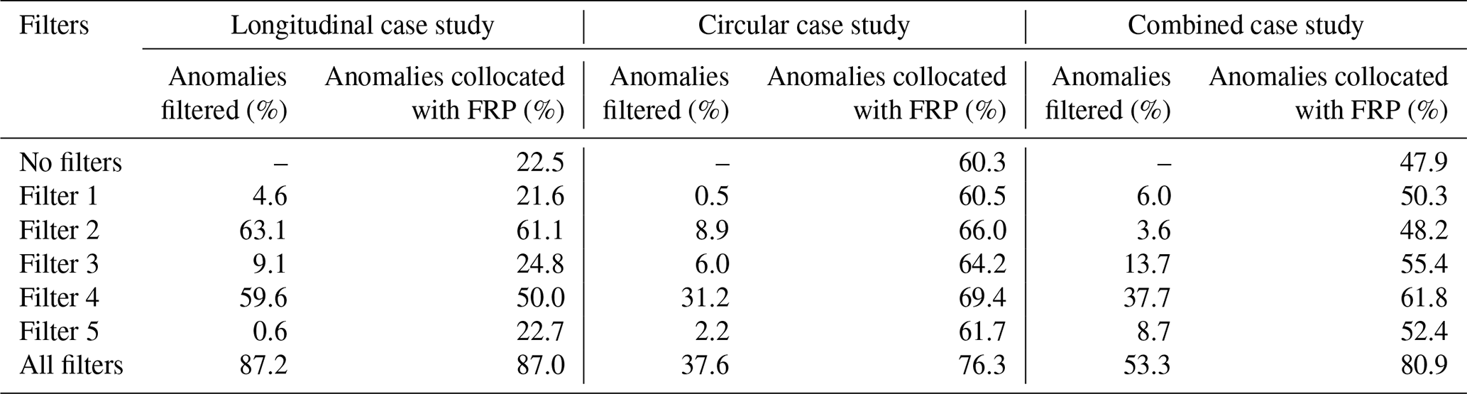
We illustrate the methodology with three days representative of the major transport regimes identified during the 2020 South American fire season. First, a “longitudinal transport” case, in which the mid-tropospheric flow is predominantly west–east across the continent, advecting air parcels coherently along lines of latitude. Second, a “circular transport” case, where the large-scale wind field forms a closed or quasi-circular pattern that recirculates air parcels above South America. Finally, a “combined transport” case, in which zonal advection and circular circulation coexist over the continent. Figure 4 displays those three case studies: the top panel shows all the 72 h back-trajectories for CO₂ anomalies greater than 4 ppm; the middle panel shows back-trajectories remaining after the filtering with those intersecting at least one fire depicted in red; the bottom panel shows the corresponding location of those fires. Table 1 summarizes, for the 3 transport regimes, the effect of the 5 successive filters on the anomalies together with the proportion of remaining trajectories crossing active fires.

3.2.1 Longitudinal transport: case study 6 August 2020 evening

Figure 4A shows the 72 h back-trajectories for MT-CO₂ anomalies detected on 6 August 2020 at the evening overpass. Two distinct transport pathways emerge. The first is a predominantly zonal flow across the South American continent, with limited mixing, favoring local contribution of South American fires to the MT-CO₂ anomalies seen by IASI. The second is a secondary circulation over the Atlantic Ocean, bringing in African emissions through long-range transport. Because these flows remain largely distinct, cross-mixing between continental and transatlantic air masses is limited. The filtering scheme efficiently identifies and removes anomalies (Fig. 4D), with 87 % anomalies filtered (Table 1). The remained anomalies are strongly collocated with South American fire activity: 87 % of the retained trajectories intersect at least one active fire (Table 1), compared to 22 % before the filters. The localization of collocated South American fires for this case, shown in Fig. 4G, highlight that most anomalies find their influence from central Amazonia linked to deforestation along the river and northern Argentinian fires linked to agricultural management. This case demonstrates that under coherent longitudinal flow and with limited mixing of flows from different influences, the method reliably isolates impact of local fire from imported contributions.

3.2.2 Circular transport: case study 1 September 2020 morning

For anomalies detected on 1 September 2020 during the morning overpass, the back-trajectories display a predominantly recirculating pattern over South America (Fig. 4B). This circulation extends the residence time of air parcels and enhances the retention of emissions in the mid-troposphere above the continent. At the same time, a distinct transatlantic flow indicates an additional influence from African sources. The filtering scheme again identifies and removes anomalies affected by this inflow, as shown in Fig. 4E. After filtering, two-thirds of the anomalies are attributed to local fire activity within the continental recirculation, while only one-third are linked to external transport (Table 1). The localization of collocated South American fires for this case, shown in Fig. 4H, highlights that most anomalies find their influence from central and northern Amazonian fires, as well as southern Cerrado fires, regions where the monthly mean FRE is high in September (Fig. 1). Overall, more than 75 % retained anomalies intersect at least one active fire, confirming that even under circular flow conditions, the method effectively limits imported signals while emphasizing the local contribution from South American biomass burning.

3.2.3 Combined transport: case study 18 October 2020 morning

Figure 4C shows the combined transport regime, characterized by predominantly longitudinal flow in the north and south of the continent, with a recirculating circulation in between. This hybrid configuration allows both the export of emissions along zonal pathways and their partial retention through recirculation, thereby reinforcing the observed CO₂ anomalies. In this case, no marked African influence is detected. Consequently, fewer anomalies are removed compared to the other regimes, with roughly half excluded after filtering. A notable feature is the elimination of anomalies finding their origins in the northern part of South America with no fires detected along their backward trajectories and transported over the Atlantic Ocean (Fig. 4F). These removed trajectories likely originated from emissions prior to the 72 h integration window and thus fall outside of the chosen temporal range of attribution, preventing potential double counting. Among the retained anomalies, about 80 % intersect at least one active fire (Table 1). Most of the remaining anomalies without fire collocation appear to result from trans-Pacific transport, although they are not flagged by the long-range filter (filter 4). Longer backward trajectories might be needed to determine if those comes from long-range transpacific transport since the west south American coast is very cloudy and might have an impact on our filter method. Overall, this case illustrates how, under complex mixed-flow conditions, the method still isolates a majority of locally driven anomalies while limiting the contribution of air masses with ambiguous or aged transport histories.

3.2.4 Synthesis of the three regimes

The three case studies illustrate how the filtering strategy consistently strengthens the attribution of mid-tropospheric CO₂ anomalies to South American biomass burning, despite differences in transport structure. Under longitudinal flow, the method is highly selective: nearly 90 % of anomalies are excluded, leaving a subset almost entirely collocated with fires. Under circular flow, the proportion of excluded anomalies is smaller, yet the filtering still demonstrates that most retained anomalies originate from continental recirculation and remain closely tied to fire activity. In the combined regime, where zonal advection and recirculation coexist, about half of the anomalies are removed, with the retained ones still dominated by local fire signatures. Taken together, these results show that the filters effectively suppress contributions from long-range or ambiguous trajectories and reliably isolate anomalies associated with South American fire sources.

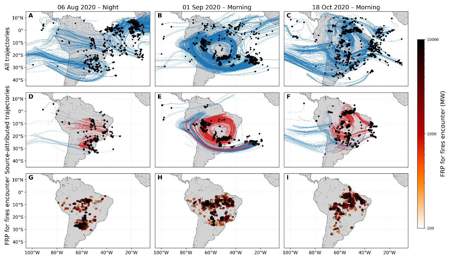
Figure 4 Case studies of mid-tropospheric CO₂ anomalies linked to South American fires. Each column shows one case study (6 August 2020 – night, 1 September 2020 – morning, 18 October 2020 – morning), and each row shows a different stage of the source-attribution procedure. Panels (A)–(C) display all backward trajectories started from the selected CO₂ anomalies for each case (blue lines), with the anomaly locations indicated by black stars. Panels (D)–(F) show only the “source-attributed” subset, i.e. trajectories that fulfil the filtering criteria and encounter at least one fire along their path; red segments mark the part of the trajectory up to the last 1° × 1° hourly aggregation of fire encounter, while blue segments correspond to trajectories with no detected fires, and black stars again mark the anomaly locations. Panels (G)–(I) display only the locations of the last fire encountered by each source-attributed trajectory. Coloured circles denote fire pixels, with marker size and colour proportional to the Fire Radiative Power (FRP) at the last encounter.

Table 1 Percentage of MT-CO₂ anomalies filtered successively by the 5 filters described in Sect. 3.1 and percentage of the remaining anomalies actually collocated with FRP for the three transport regimes.

4 Generalization to 2020 South American fire season

The methodology described in Section 3 is now applied to the full South American fire season of 2020 (1 August–31 October). Using our filtering procedure, about 66 % of the detected anomalies are considered as coming from long-range transport or unknown origin for the whole period, and about 75 % of the retained anomalies are collocated with hourly fire detections (see Table S1 in the Supplement). This distribution is globally consistent with the percentage obtained for the 3 case studies in Sect. 3.2.

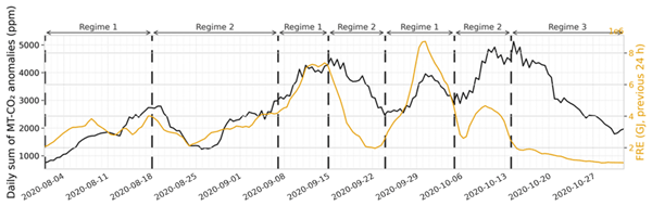
Once the CO₂ anomalies attributed to long-range transport have been removed, the CO₂ anomalies identified as originated from local emissions can be compared to the observed fire activity. For that aim, the three transport regimes characterized in Sect. 3.2, longitudinal (Regime 1), circular (Regime 2), and combined (Regime 3), are used here as an interpretative scaffold to analyze the co-variability between fire activity, expressed as Fire Radiative Energy (FRE, in GJ, integrated over the preceding 24 h), and the sum of mid-tropospheric CO₂ anomalies (in ppm) derived from IASI.

Figure 5 shows the time series of the daily sum of mid-tropospheric CO₂ anomalies derived from IASI morning and evening overpasses (in black), smoothed using a 72 h moving average over South America during the 2020 fire season. The anomalies are compared to the total FRE (in orange) from GOES-16 observations, integrated over South America and computed 24 h prior to each IASI observation to account for transport time. FRE values are also smoothed using a 72 h window. FRE exhibits four main episodes of enhanced fire activity: two moderate peaks in August, a first major peak in mid-September, a second major peak in late September–early October, and a final peak in mid-October occurring only a few days after the previous one. Overall, the sum of CO₂-anomaly follows the same variations, indicating a strong link between the two variables. However the amplitude of the signal differs, mainly driven by the atmospheric transport dynamic as identified in Sect. 3: longitudinal (Regime 1) from early August to about 19 August, again from 9 to 16 September, and from 29 September to 6 October; circular (Regime 2) from about 19 August to 9 September, from 16 to 29 September, and from 6 to 14 October; and finally combined (Regime 3) from about 14 October to the end of the month. Because these regimes control both export and residence time in the mid-troposphere, they directly affect how the fire signal appears in the CO₂ anomalies.

The first part of the season is dominated by longitudinal transport. The flow is mainly zonal, long-range mixing is limited, and export from the continent is efficient. During this phase, the sum of CO₂-anomaly rises and falls almost synchronously with FRE, as expected for a regime with little recirculation. After the second August peak, the circulation shifts to circular and FRE drops rapidly. Under this regime, residence times over the subcontinent increase and air masses recirculate over the continent. Consequently, while FRE decreases strongly at the end of August, the CO₂-anomaly sum decreases more slowly, because emissions from the preceding peak are not exported from the region.

From late August to the first days of September, FRE increases nearly steadily. The CO₂-anomaly sum also increases, but the rise is slightly delayed compared with FRE, which is consistent with the presence of circular transport during this interval. The situation changes again in the second week of September, when the flow returns to longitudinal and FRE reaches one of the largest peaks of the season. In this longitudinal phase, the anomalies follow the FRE variations very closely and reach high values. Immediately after the peak, the circulation switches back to circular transport, FRE decreases markedly, and the CO₂-anomaly sum remains elevated and declines only gradually until the end of the third week of September.

A new longitudinal period, from late September to early October, coincides with the largest fire episode of the season in terms of radiative energy. Here again the effect of the regime is very clear: the CO₂-anomaly sum responds without lag and reproduces the entire rise, peak and fall of the corresponding FRE variations. Yet the corresponding anomaly maximum is smaller than the mid-September one, despite the higher FRE.

About one week later, in mid-October, a peak episode is observed, this time under a circular regime. Both FRE and the CO₂-anomaly sum increase again, but the CO₂ anomalies reach very high levels even though FRE is lower than during the previous two peaks. This behavior can be explained by the recirculation and retention of the emissions released during the late-September/early-October event combined with the short time interval between the two peaks, preventing the mid-tropospheric CO₂ from returning to background values. Finally, the post-peak period takes place under a combined regime, which still favors recirculation of the air masses affected by the earlier events but also contains a longitudinal component that transmits day-to-day variability. During this period, FRE decreases monotonically towards the end of October, while the CO₂-anomaly sum decreases more slowly and remains elevated for several days.

To investigate how the transport regime influences the relationship between CO₂ anomalies and FRE, Fig. 6 displays a scatter plot of these two variables, with each transport regime represented by a distinct color. The correlation between CO₂ anomalies and FRE is computed separately for each transport regime.

Under longitudinal (Regime 1) transport, the points form a clear positive relationship with a high correlation (r=0.88). The dispersion is limited, indicating that when export dominates while mixing and recirculation is weak, day-to-day emissions from fire activity are efficiently transferred to the mid-troposphere. This behavior is consistent with the parts of the time series where FRE and CO₂ co-evolve most clearly, i.e. the mid-September and late-September/early-October peaks, and, to a lesser extent, the mid-August peak.

Under circular (Regime 2) transport, the scatter becomes broader and is shifted upward for low-to-moderate FRE values, and the correlation is lower (r=0.54). For a given FRE, the CO₂-anomaly sum is often higher than under Regime 1 because the air mass still contains CO₂ emitted during previous, more active days, and because Regime 2 tends to introduce a lag in the anomaly response. This is exactly the situation observed after the September and October peaks, when FRE decreases quickly but the anomalies remain high. Also, the part of the circular regime that matches the closest longitudinal regime efficiency corresponds to August levels where the radiative energy was at its lowest, reducing the emissions and though reducing the impacts of recirculation.

Under combined (Regime 3) transport, the relationship is also very tight, with a high correlation (r=0.97) and a pronounced positive slope, even though FRE values are lower than earlier in the season. This configuration corresponds to a situation with a high background inherited from the succession of September–October peaks, but in which the longitudinal component of the flow still organizes day-to-day variability, so even relatively small changes in FRE remain visible in the anomaly sum. This is characteristic of the late October period.

Taken together, the time series and the scatter analyzed for each transport regime show that mid-tropospheric CO₂ anomalies over South America in 2020 were driven by fire activity but with a relationship depending on the transport type. Peaks in FRE were systematically mirrored in the anomaly sum, confirming the link between surface fire activity and the corresponding detected atmospheric signal, while the slower post-peak decay of CO₂ was explained by the occurrence of circular and, later, combined regimes that recirculated and retained the fire-enriched air masses.

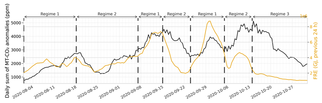
Figure 5 Time series, smoothed using a 72 h window, of the daily sum of mid-tropospheric CO₂ anomalies derived from IASI morning and evening overpasses (black), over South America during the 2020 fire season and of total FRE (orange) from GOES-16 observations, integrated over South America and computed 24 h prior to each IASI observation to account for transport time. The “Regime” delimiters highlight three representative atmospheric transport regimes periods: Regime 1 for longitudinal regime, Regime 2 for circular regime, and Regime 3 for combined regime.

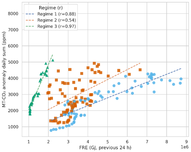
Figure 6 Daily sum of mid-tropospheric CO₂ anomalies (ppm) vs. Fire Radiative Energy (FRE, GJ) for three transport regimes: longitudinal transport (blue), circular transport (orange), and combined transport (green). Pearson correlation coefficients “r” are indicated for each transport regime.

5 Discussion

The analysis of the 2020 South American fire season shows that intense biomass burning leaves a clear and quantifiable imprint on mid-tropospheric CO₂ as observed by IASI. After removing trajectories affected by long-range or ambiguous transport, roughly 75 % of the remaining anomalies over South America and adjacent oceanic basins are collocated with active fires, and the sum of CO₂ anomalies at 8–11 km co-varies tightly with Fire Radiative Energy integrated over the preceding 24 h. The strength and form of this relationship depend on the large-scale circulation. In particular, when zonal export dominates (longitudinal regime), the correlation between FRE and the anomaly sum is very high and the dispersion is small, indicating that day-to-day variations in fire activity are efficiently transmitted to the mid-troposphere. Under circular and combined regimes, recirculation and residence time modulate the amplitude and timing of the response, which extends the decline of the sum of the CO₂ anomalies toward its background level, particularly after peaks. Taken together, these results provide a direct attribution of mid-tropospheric CO₂ anomalies to biomass-burning emissions while accounting for proper horizontal transport and confirm that a substantial fraction of the variability in the 8–11 km partial column can be explained by recent fire activity. However, the amplitude of the atmospheric response is not determined by FRE magnitude alone, but also by fuel type, size, density, moisture content, and local meteorology (Lawson et al., 2015; van Leeuwen and van der Werf, 2011) and by the efficiency of the vertical transport that injects fire emissions into the mid-troposphere (Rio et al., 2010; Tang et al., 2022). Beyond fire radiative energy, the amplitude of the mid-tropospheric response is governed by fuel load and type, moisture content and combustion phase, and by the meteorological modulation of injection efficiency through atmospheric instability, which evolves through the season. A promising route to disentangle these controls is a multi-species approach: the co-emitted CO and CH₄ retrieved from IASI alongside CO₂ would allow joint constraints on injection heights and emission types across tropical biomes, linking the strong, easily tracked CO signal to the weaker CO₂ anomalies studied here. That can explain the amplitude differences between CO₂ anomalies response and FRE for peaks. We deliberately work with the daily sum of CO₂ anomalies rather than their means because intense fires and pyroconvective plumes both create strong local enhancements and promote the accumulation of anomalies over extended areas and time scales (Freitas et al., 2006; Peterson et al., 2022); the mean tends to dilute this combined effect and does not capture the co-evolution with FRE as clearly. At the same time, the use of the sum raises the question of how sensitive this metric is to the satellite sampling itself, since cloud cover and viewing geometry limit the number of available retrievals within a plume.

The altitude range sampled by IASI is central to the interpretation of these findings. IASI vertical weighting functions peak near 8–11 km (Fig. 1), with negligible sensitivity below about 4 km. This means that the anomalies we interpret related to fire do not reflect boundary-layer or lower-tropospheric variability, but the excess CO₂ that has been transported high into the free troposphere. Over tropical South America, the top of the convective boundary layer rarely exceeds a few kilometers (Chédin et al., 2005; Darbyshire et al., 2019), and “ordinary” shallow or deep convection is not sufficient to inject large amounts of combustion products to 8–11 km at daily temporality (Deeter et al., 2018; Gonzalez-Alonso et al., 2019). The persistence of strong, spatially coherent IASI anomalies at these altitudes, tightly tied to FRE, therefore implies the occurrence of vigorous convective processes directly coupled to fires. This is consistent with the pyroconvection process, whereby the intense sensible and latent heat released by large, high-intensity fires triggers or amplifies deep convection (Muth et al., 2024; Paugam et al., 2016; Tedim et al., 2018), generating plumes that can overshoot the freezing level and lift smoke, aerosols and trace gases into the mid- and upper troposphere (Couto et al., 2024; Cussac et al., 2020). In this context, the FRE–CO₂ relationship documented here can be interpreted as the signature of pyroconvective injection: large FRE episodes in fire-prone biomes such as southern Amazonia, the Cerrado, the Pantanal or northern Argentina favor the formation of pyroconvective plumes that uplift CO₂-enriched air masses to altitudes where IASI is most sensitive. The efficiency of this injection is not fixed through the season: the fraction of fires reaching the free troposphere rises through the season as atmospheric stability decreases from ∼ 3 %–20 % over the Amazon in the mean to ∼ 15 %–40 % late in the season (Gonzalez-Alonso et al., 2019), so that fires need progressively less energy (FRE) to be lofted as the season advances, consistent with the persistence of strong anomaly–FRE coupling at comparatively lower FRE late in the season. We also note that 2020 was an exceptionally intense South American season (Garcia et al., 2021; Silveira et al., 2022), so the lofted signal and its detectability by IASI are likely larger than in a climatologically average year.

This interpretation has direct implications for how biomass-burning emissions and their vertical distribution are represented in global atmospheric CO₂ models. As an illustration, we first compare the CAMS v23r1 CO₂ product from the global inversion of optimised greenhouse gas fluxes (Chevallier, 2023) with the observed IASI anomalies. This model provides globally consistent CO₂ surface fluxes and 3-hourly concentrations from an atmospheric inversion constrained by in situ observations but does not include an explicit representation of fire-driven pyroconvective uplift. When we compare the anomaly fields derived from IASI with the corresponding IASI-weighted CO₂ partial column computed from this CAMS inversion system (Fig. 7A and B), the model fails to reproduce both the amplitude and the spatial structure of the observed MT-CO₂ anomalies, while accounting for large CO₂ anomalies at the surface (Fig. 7D) that correlates to a given extent to fire activities (Fig. 7C). The most pronounced plumes seen by IASI, especially those associated with the major September–October fire episodes, are not simulated in CAMS fields. This suggests that, if emissions are injected too low into the column by the underlying transport model, even large flux corrections will not generate the observed CO₂ increase at 8–11 km. The comparison with CAMS therefore points to missing or misrepresented processes rather than a simple flux bias. In particular, it indicates that including in atmospheric transport models the vertical coupling between intense fires and deep convection, through pyroconvective transport, is crucial to properly account for fire emissions in local and global carbon budget estimation.

A natural question is whether a model that does represent fire-driven vertical transport reproduces the anomalies. We therefore repeated the comparison against the CAMS EGG4 greenhouse-gas reanalysis, which assimilates IASI CO₂ and distributes GFAS biomass-burning emissions in the vertical using Plume-Rise-Model injection heights (Fig. 8). For a representative day (1 September 2020), the EGG4 surface CO₂ field (Fig. 8d) is in fact richer and more fire-resolved than that of the inversion, with enhancements exceeding 100 ppm over southern Amazonia and the Pantanal that closely track the Fire Radiative Energy field (Fig. 8c). Yet the corresponding IASI-weighted mid-tropospheric field (Fig. 8b) is essentially indistinguishable from that of the IASI-independent inversion and reproduces none of the coherent 8–11 km anomalies observed by IASI (Fig. 8a). Two conclusions follow. First, although EGG4 assimilates IASI CO₂, the assimilation leaves no visible imprint on the mid-tropospheric field, consistent with the large, fire-driven departures being down-weighted or rejected by the variational quality control. Second, and independently, the fire signal that EGG4 clearly represents at the surface does not reach the free troposphere: the GFAS Plume-Rise-Model injection heights are known to be biased low (Rémy et al., 2017; Tang et al., 2022), so emissions are deposited too low in the column and never populate the 8–11 km layer. The comparison therefore shows the two limitations side by side, a surface field that resolves the fires but neither an assimilation imprint nor a vertical transport that carries the signal aloft, indicating that the limitation is not a missing process but the fidelity with which that process is represented and constrained.

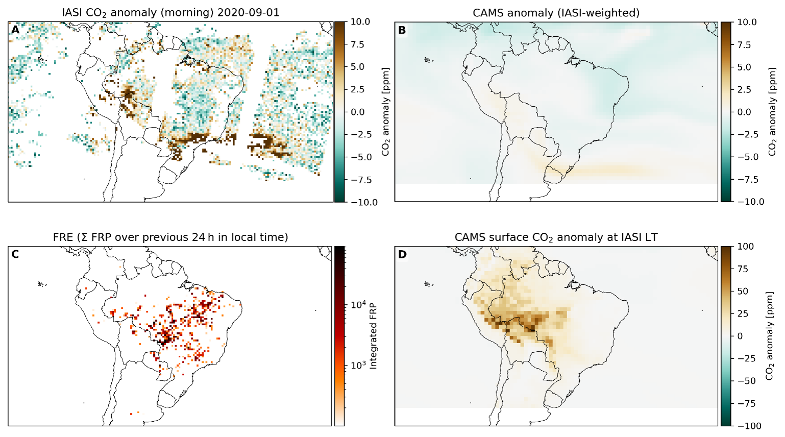
Figure 7 Spatial comparison of satellite- and model-based CO₂ anomalies and fire activity over South America for 1 September 2020 (morning overpass; ∼ 09:30 local solar time). (A) Gridded IASI mid-tropospheric CO₂ anomaly (ppm). (B) CAMS CO₂ anomaly for the IASI-weighted partial column, sampled at the IASI local overpass time and expressed on the same anomaly scale as (A) (ppm). (C) Fire Radiative Energy proxy computed as the sum of GOES-16 Fire Radiative Power (FRP) accumulated over the 24 h preceding the overpass in local time, aggregated on a 0.5° grid and displayed on a logarithmic scale. (D) CAMS surface CO₂ anomaly at the IASI local overpass time (ppm).

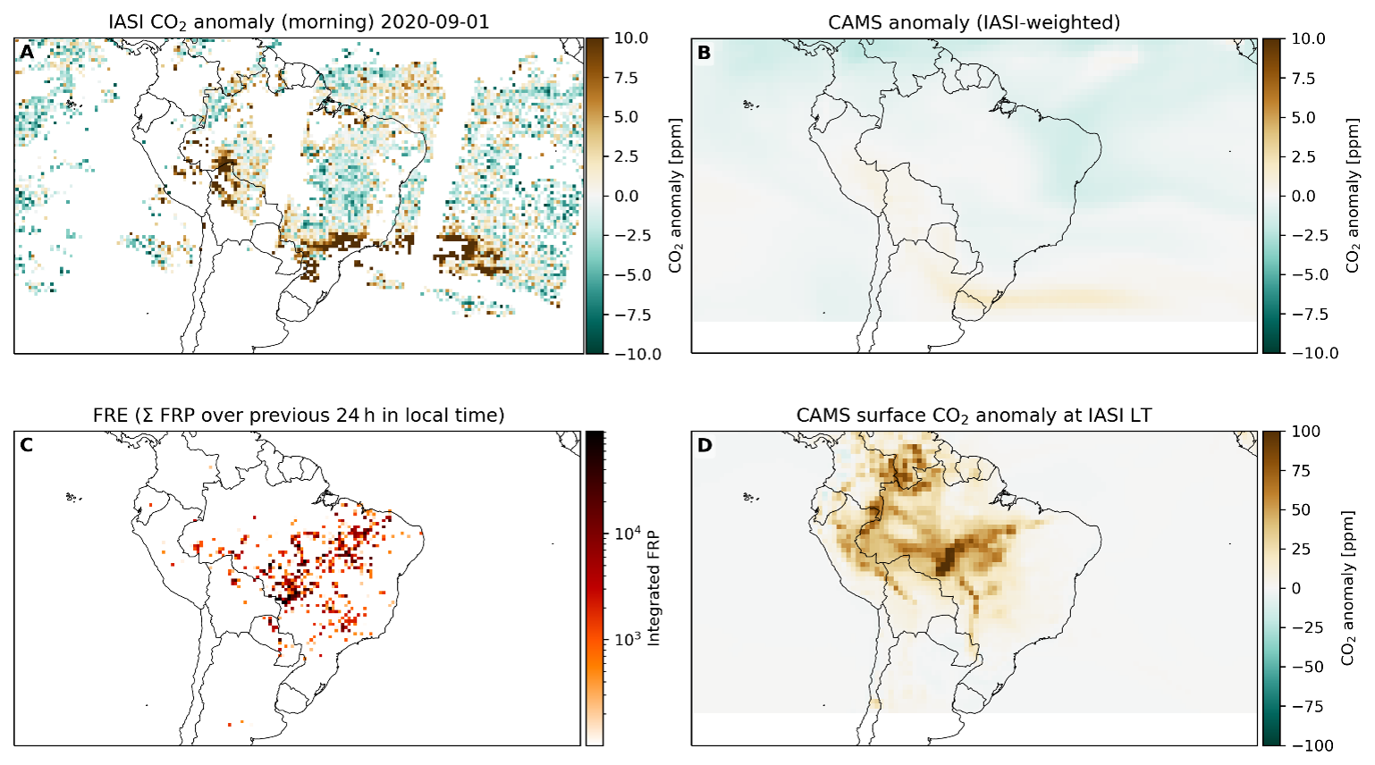
Figure 8 Comparison between IASI mid-tropospheric CO₂ anomalies and the CAMS EGG4 reanalysis for a representative day (1 September 2020). (A) IASI-observed MT-CO₂ anomaly (morning overpass); (B) EGG4 IASI-weighted MT-CO₂ partial-column anomaly; (C) Fire Radiative Energy (Σ FRP over the preceding 24 h); (D) EGG4 surface CO₂ anomaly at the IASI local overpass time.

6 Conclusions

In this study, we have developed a methodology to relate daily mid-tropospheric CO₂ anomalies observed at 8 to 11 km level, to South American fire activity during the 2020 burning season, including the consideration of horizontal transport. We first constructed a dynamic, latitude- and time-dependent background to isolate MT-CO₂ anomalies in the 8–11 km layer, gridded them at 0.5° daily resolution, and selected strong events exceeding 4 ppm. We then computed 72 h backward trajectories with LAGRANTO using ERA5 winds, applied a series of filters to remove trajectories influenced by long-range or ambiguous transport, and finally collocated the remaining trajectories with GOES-16 Fire Radiative Power fields. This combination of anomaly definition, Lagrangian transport, and fire collocation provides a coherent methodological framework to attribute MT-CO₂ anomalies to recent and local biomass burning while explicitly accounting for horizontal transport and flow regimes.

The study exploits the complementary strengths of IASI and GOES-16. IASI provides twice-daily, cloud-filtered measurements of CO₂ in a mid-tropospheric partial column, with a vertical sensitivity peaking in the free troposphere at 8 to 11 km, so that MT-CO₂ anomalies reflect the integrated effect of emissions of CO₂ that have been transported to this tropospheric layer. In contrast, GOES-16 offers quasi-continuous geostationary monitoring of Fire Radiative Power at high temporal resolution, which we aggregate in space and time to derive daily Fire Radiative Energy as a proxy for the intensity and timing of surface biomass burning. The synergy between a nadir-sounding infrared spectrometer and a geostationary fire imager is central to our approach: while IASI alone cannot distinguish between locally generated and remotely transported anomalies, and GOES-16 alone cannot track the fate of emitted CO₂ above the boundary layer, their joint use through Lagrangian trajectories allows us to connect the location, timing and magnitude of fires with their imprint in the mid-troposphere.

Once horizontal transport is explicitly represented, a substantial fraction of the day-to-day variability of mid-tropospheric CO₂ over tropical South America can be directly attributed to recent local fire activity, and that the largest MT-CO₂ anomalies reflect episodes of vigorous, likely pyroconvective, injection of combustion products into the free troposphere. The relationship between FRE and MT-CO₂ anomalies thus emerges as an observational fingerprint of fire-driven vertical coupling between the surface and the mid-troposphere at 8 to 11 km, highlighting that MT-CO₂ anomalies from IASI contain quantitative information on both the timing and intensity of tropical biomass burning that is currently under-exploited in global carbon budget inversions. A natural extension is to move from establishing the FRE–anomaly link to attributing individual anomalies to specific fires: because a given anomaly typically intersects several fire aggregations along its trajectory, robust per-fire attribution would require an explicit injection-probability model, for which a CAPE/CIN-based convective indicator is a promising ingredient. Such per-fire attribution would in turn enable the linkage of vegetation and plume types and the study of the diurnal evolution of pyroconvection.

To properly evaluate fire emissions, and their contributors, from MT-CO₂ anomalies would require using a full atmospheric modelling framework that represents pyroconvective injection faithfully. Our comparisons indicate that this is not achieved simply by including a pyroconvection scheme: an inversion without injection physics misses the anomalies entirely, and even an injection-height-aware, IASI-assimilating reanalysis (EGG4) reproduces them only at the surface. Closing this gap will likely require both stronger observational constraints on the lofted fraction, of the kind the IASI MT-CO₂ anomalies provide, together with improved injection-height estimation, and higher-resolution, convection-resolving transport; the higher-resolution CAMS global greenhouse-gas forecast is a natural candidate for such tests but became available only from 2024 and so could not be applied to the 2020 season studied here. This would also be needed to overcome several limitations of the study. First, clouds do impact the number of available observations from IASI and precludes studying areas with persistent cloudiness such as on the West coast of South America. Gaps in the observations also imply that the daily sum of MT-CO₂ used in the study may underestimate the actual accumulation of CO₂ in the mid-troposphere. GOES-16 FRP may also be affected by clouds, but it is less critical than for IASI. Second, limiting back-trajectories to 72 h precluded accounting properly for CO₂ anomalies that would find their origin in Africa or Australia. The threshold of 100 MW applied to FRP to isolate fires that may trigger injection of CO₂ up to the attitude range seen by IASI could also be refined and linked to specific burning conditions and fuel type.

Nevertheless, despite the simplicity of the assumptions used here, this study shows that intense biomass burning can exert a strong, rapidly varying impact on the highest-altitude mid-tropospheric CO₂ and demonstrates that a faithful representation of pyroconvective transport and, where it cannot be resolved, observational constraints on the lofted fraction, is essential for constraining fire emissions and their role in the carbon cycle. Extending the study to co-emitted gases CO and CH₄ also retrieved from IASI (Crevoisier et al., 2009, 2013; George et al., 2009; Thonat et al., 2015) would enable a multi-species constraint on both the injection heights and the emission types of various tropical biomes.