Hydrological drivers of hydrogen cyanide wildfire emissions from Indonesian peat fires during the 2015, 2019, and 2023 El Niño events

Indonesian peatlands store vast amounts of carbon that are highly vulnerable to fire during El Niño-driven droughts. When ignited, peat releases large quantities of greenhouse gases and other species with significant environmental impacts, including hydrogen cyanide (HCN), a sensitive tracer of smouldering combustion. In this work, we use new satellite retrievals from the Infrared Atmospheric Sounding Interferometer (IASI) spectra using the University of Leicester IASI retrieval scheme (ULIRS), that we validate against ground-based Fourier transform infrared (FTIR) measurements at Reunion Maido, TOMCAT atmospheric model simulations, hydrological information, and fire activity observations to evaluate the factors driving trace gas emissions during the 2015, 2019, and 2023 El Niño events.

The 2015 El Niño produced large burdens of HCN and carbon monoxide (CO), unprecedented in the satellite observational era and driven by exceptionally low soil moisture, depressed groundwater levels, and deep burn depths. In contrast, the 2019 and 2023 events exhibited markedly weaker emissions despite similar Oceanic Niño Index (ONI) anomalies, reflecting more favourable hydrological conditions. Comparisons of the satellite trace gas observations with simulations of the TOMCAT model show that burned-area-based inventories such as the Global Fire Emissions Database (GFED) version 4 substantially overestimate emissions from peat fires in 2015, while a new peat-specific database, FINNpeatSM (Fire Inventory from NCAR (FINNv1.5) New peat with Soil Moisture), better represents fire season timing and burn depth by incorporating soil moisture constraints. From satellite-derived HCN : CO enhancement ratios, we provide new emission factors for HCN that offer benchmarks for new emission inventories.

Our results show that peat fire intensity and emissions are driven not only by El Niño strength but also by local hydrological conditions such as soil water content and precipitation. Integrating hydrological indicators with satellite observations of atmospheric composition is therefore critical for improving fire emission inventories.

1 Introduction

During the South-East Asian dry season, El Niño generally has a strong influence on the conditions driving widespread fires. Fires are commonly used across the region for land clearing to manage fields and prepare the soil for the growing season. However, much of the land in Kalimantan and Sumatra, Indonesia, is underlain by tropical peat soils that have been extensively drained using a network of canals. Dry conditions and elevated temperatures, typical of the dry season, are particularly exacerbated in the Indonesian environment during El Niño, making man-made fires more difficult to control (Parker et al., 2016). Under these conditions, vegetation fires can ignite the underlying carbon-rich peat soils, causing wildfires that are extremely difficult to extinguish and can burn for weeks.

Indonesian peatlands occupy about 55 % of the tropical peatland carbon reservoir (Dargie et al., 2017; Page and Hooijer, 2016). They store extremely large amounts of partially decayed organic matter, and release substantial amounts of pyrogenic trace gas species and particulate matter into the atmosphere when burned. The carbon stored can be emitted in the form of trace gases such as carbon dioxide (CO₂), CO and HCN, the latter also badly affecting the air quality across South-East Asia (Watson et al., 2019). In particular, during El Niño years strong peaks in global HCN have been observed (Park et al., 2021; Rosanka et al., 2021), suggesting that it is a good atmospheric tracer for peat fire (Pumphrey et al., 2018; Sheese et al., 2017). Monitoring HCN emissions is therefore important in understanding severe peatland fires, and for understanding global carbon accounting.

Peatlands are particularly vulnerable to smouldering fires, which are characterised by slow, low-temperature, flameless combustion. Peat fires typically develop in three stages (Usup et al., 2004). In the first, surface peat is ignited by a surface fire event. In the second stage a smouldering front burns laterally and downward into the surface (up to 20 cm), and in the third the smouldering extends into deeper peat layers below 20 cm in depth. It is the latter smouldering stages in which HCN is primarily released. Ultimately, it is the peat soil moisture, in particular the ground water level (GWL), that determines the ignition and spread of these smouldering fires.

During the period September to November 2015, under the influence of a strong El Niño, Indonesia experienced the most severe wildfire season of the last three decades. The intensity of the 2015–2016 El Niño event (ONI: +2.6 °C) was comparable to the 1997–1998 El Niño (ONI: +2.4 °C) (Barnston et al., 1997; Huang et al., 2017), one of the strongest recorded (Field et al., 2016; Santoso et al., 2017). The peatland fires lasted for about three months during which more than 2.6 Mha of forest, peat and other land types were burned, and an equivalent of 5 % of the global 2015 fossil fuel CO₂ emissions were released (Vetrita and Cochrane, 2020). In the period 1997–2016, fires in equatorial Asia and particularly Indonesia produced about 8 % of the global fire carbon emissions (van der Werf et al., 2017).

The 2023–2024 El Niño period is currently the second strongest event of this century (ONI: +2.0 °C), falling just behind that of 2015–2016. However, as will be shown, there is a marked difference in the behaviour of the fire plumes and the amount of HCN released. While previous studies have documented the role of El Niño in intensifying Indonesian fire activity (Field et al., 2016; Whitburn et al., 2017; Nurdiati et al., 2021), large uncertainties remain in quantifying trace gas emissions from peatland combustion, particularly for HCN, a key tracer of peat fires.

Existing fire inventories, such as GFEDv4, rely primarily on burned-area estimates that are poorly suited to capturing underground peat combustion, leading to biases in both the timing and magnitude of emissions. These discrepancies often stem from uncertainties in burned carbon estimates, particularly in peatlands (Nechita-Banda et al., 2018; Lohberger et al., 2018). Peat extent and depth estimation remain highly uncertain in Indonesia (Hooijer and Vernimmen, 2013), and may also reflect inaccuracies in biome attribution.

In this paper, we systematically compare multiple El Niño events to evaluate the influence of large-scale climate forcing and local hydrological parameters on peat fire dynamics. We provide new satellite-based constraints on HCN emission factors, evaluate the performance of the GFED emission inventory, introduce a new database based on the method developed for FINNpeatSM (Kiely et al., 2019), and assess how variations in soil moisture and groundwater level influence interannual differences in wildfire dynamics and emissions.

The paper is structured as follows. Section 2 describes the main datasets and models used in this study, including IASI CO and HCN from ULIRS. In Sect. 3.1, the IASI CO and HCN retrievals are compared with ground-based Fourier transform infrared (FTIR) measurements at the Reunion Maido NDACC station. In Sect. 3.2, we investigate HCN emissions during the 2015 Indonesian fire season using total columns retrieved with the ULIRS, and compare with recent TOMCAT model simulations (Bruno et al., 2022, 2023). In this section, we also propose a new estimate of HCN emission factors by calculating the enhancement ratio between HCN and CO, ER${}_{\mathrm{HCN}/\mathrm{CO}}$. Section 3.3 discusses the differences between the 2015, 2019, and 2023 fire seasons and explores their underlying causes, focusing on soil moisture and precipitation as the principal hydrological drivers of fire activity, using the FINNpeatSM approach (Kiely et al., 2019). Finally, Sect. 4 synthesizes the main findings of this work and highlights the implications of hydrological controls for peatland fire dynamics and trace gas emissions.

2 Data

This section presents the suite of complementary satellite observations, ground-based measurements, reanalysis products, and emission inventories used to characterise the variability of CO and HCN during three recent Indonesian fire seasons (2015, 2019 and 2023) influenced by El Niño. The atmospheric composition is primarily constrained using spaceborne thermal infrared retrievals from IASI and ground-based FTIR observations at the NDACC Maido station, whereas chemical transport model simulations from the TOMCAT model provide a framework for interpretation. To investigate the hydrological drivers of fire activity and peat combustion, satellite-derived precipitation (IMERG), surface and subsurface soil moisture products (SMAP and SWI), and ERA5 wind fields have been used. In particular, precipitation and SWI temporal variability over Indonesia is used to show the influence of the moisture content of the soil on fire emissions, and the SMAP data are used to produce an enhanced emission database that well represents peat fire emissions. Fire occurrence and emissions are quantified using global (GFED4) and regionally enhanced (FINNpeatSM) inventories, together with high-resolution active fire detections from VIIRS. The combined use of these datasets enables the evaluation of fire emissions, atmospheric transport, and the role of moisture conditions in modulating trace gas emissions over Indonesia and the tropical Indian Ocean.

2.1 Atmospheric CO and HCN data

2.1.1 IASI

IASI is a hyperspectral sounder onboard the three polar-orbiting MetOp satellites, launched in 2006 (IASI-A, now decommissioned), 2012 (IASI-B), and 2018 (IASI-C) jointly by CNES (Centre National d’Études Spatiales) and EUMETSAT (European Organisation for the Exploitation of Meteorological Satellites). The main objective of IASI is to provide a continuous and long-term collection of measurements to support meteorology, namely temperature and humidity tropospheric profiles with high vertical resolution and precision, but it has also been used to monitor both the environment and climate on a global scale through observations of atmospheric composition (Clerbaux et al., 2009; Hilton et al., 2012).

IASI measures the spectrally resolved thermal infrared radiation emitted by the Earth and the atmosphere system at the top of the atmosphere (TOA) across the spectral range 645 to 2760 cm⁻¹ at a spectral resolution of 0.5 cm⁻¹ and spectral sampling of 0.25 cm⁻¹. Due to its high spectral resolution and spectral sampling, IASI is able to measure a large number of trace gases, including some species observed only sporadically in the measured spectra (Clerbaux et al., 2009; Clarisse et al., 2011). These species include 10 gases with clear spectral signatures that are always present in the satellite measurements, CO₂, N₂O, CFC‐11, CFC‐12, OCS, H₂O, CH₄, O₃, CO and HNO₃ (Clarisse et al., 2011; Clerbaux et al., 2009) and 14 reactive trace gases. Some of these reactive gases are the typical products of biomass burning, such as HCN, which has been assessed in previous IASI studies, and is retrieved using the absorption band centred at ∼ 712 cm⁻¹ (ν₂ band) (Coheur et al., 2009; De Longueville et al., 2021; Duflot et al., 2015, 2013).

The sensitivity of IASI retrievals near the surface is limited and exhibits a strong dependence on thermal contrast (with large differences between daytime and nighttime), which constrains the amount of vertical information that can be obtained. For CO, the averaging kernels indicate two distinct vertical contributions: one from the lower troposphere, peaking on average at about 5 km, and another from the upper troposphere, near 10 km. The top panels of Fig. 1 show the CO averaging kernels (solid lines) and total column averaging kernel (dashed lines) for IASI measurements on 2 November within the wildfire plume (110° E, 14.5° S) and outside the plume (95.4° E, 35° S). In contrast, HCN retrievals are primarily sensitive to the mid to upper troposphere, with peak sensitivity between 9 and 12 km, as shown in the bottom panels of Fig. 1 reporting HCN averaging kernels (solid lines) and total column averaging kernel (dashed lines) for in-plume and out-of-plume scenarios.

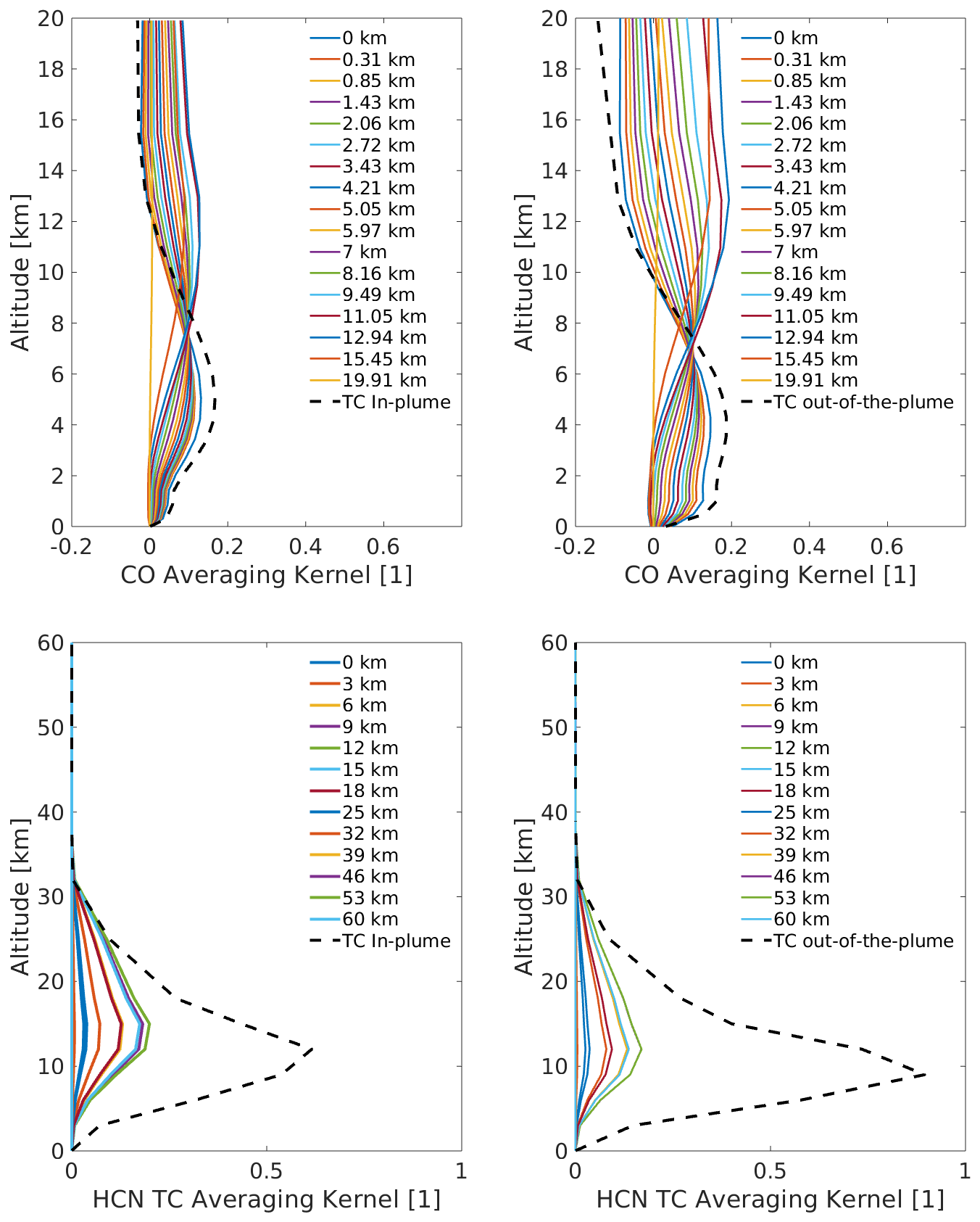
Figure 1 CO (top panels) and HCN (bottom panels) averaging kernels and total column averaging kernel for IASI measurements on 2 November withing the wildfire plume (110° E, 14.5° S) and outside the plume (95.4° E, 35° S).

2.1.2 Retrieval algorithm

The concentrations of HCN and CO during the 2015, 2019 and 2023 fire seasons were retrieved using the University of Leicester IASI Retrieval Scheme (ULIRS). The ULIRS scheme is a retrieval algorithm originally developed at the University of Leicester and subsequently by the UK National Centre for Earth Observation to study tropospheric trace gas concentrations from IASI satellite measurements. Here we examine results for carbon monoxide and hydrogen cyanide under clear sky and partially cloudy conditions from the radiances measured by the IASI instrument. A full description of the ULIRS and a summary of the main features are given in Illingworth et al. (2011a, b), with relevant updates outlined in this work. In essence, the ULIRS retrieves atmospheric trace gas partial and total column information from IASI top-of-atmosphere radiances. To do this, the scheme incorporates an optimal estimation method (Rodgers, 2000) to constrain the inversion with a priori information about the variables to be retrieved, in this case CO and HCN, alongside H₂O, CO₂ and temperature (profile and surface).

The CO retrieval setup largely follows the setup of Illingworth et al. (2011a) but with a single global average a priori profile constructed with ACE v3.6 data (Bernath et al., 2021) covering 2004 to 2018 for the stratospheric profile at one-sigma uncertainty (above 15 km). This was merged with the troposphere (below 15 km) using TOMCAT model data over the 2006 to 2015 period. The number of retrieval levels compared to Illingworth et al. (2011a) was also reduced to 17 equidistant pressure levels from the surface up to 50 hPa. The ULIRS CO utilises optimal estimation in common with other IASI schemes such as FORLI-CO (Fast Optimal Retrievals on Layers for IASI) which produces the operational CO product for the EUMETSAT AC-SAF. The main difference being in their vertical grids, a priori assumptions, and forward modeling methods. Both schemes use look-up-tables of absorbances to speed up the radiative transfer calculations.

The HCN retrieval employs a fixed altitude grid with 13 levels, 3 km spacing from 0 to 18 km with levels then at 7 km spacing up to and including 60 km. Due to the weak HCN absorption, ULIRS retrievals are calculated in a limited spectral region, 710–715 cm⁻¹, containing the ν₂ band of HCN in order to avoid interferences from the absorption of other species in the spectrum, in particular avoiding line mixing effects of a CO₂ Q branch centred near 720 cm⁻¹. Only 11 selected spectral channels are used in the process: 710.25, 710.50, 710.75, 712.50, 712.75, 713.50, 713.75, 714.00, 714.25, 714.75, 715.00 cm⁻¹. The a priori profile was constructed from INTEX-B aircraft information (Singh et al., 2009) in the troposphere and ACE v4 data (Boone et al., 2020) in the stratosphere over polluted scenes. A loose constraint on the HCN a priori uncertainty of 100 % was assumed. Here we limit both the CO and HCN retrievals to a maximum of 10 iterations. Other schemes that produce HCN products from IASI include the ANNI (Artificial Neural Network for IASI) (Duflot et al., 2013), which provides rapid, global, total column mapping. While ULIRS retrievals often have a Degrees of Freedom for Signal (DOFS) near 1 for HCN, suggesting limited strict vertical profiling, the scheme still provides sensitivity to broad vertical distributions rather than a fixed total column. This allows for analysis of vertical partitioning and high-altitude transport (e.g., biomass burning plumes) in the troposphere.

ULIRS makes use of the Reference Forward Model (RFM), a line-by-line (LBL) radiative transfer model developed at the University of Oxford (Dudhia, 2017), which can be used to simulate the TOA spectrum as measured by a spaceborne sensor. Line-by-line methods for numerically solving RT equations, such as the RFM, can be time-consuming and require large computational power. Retrieval schemes generally require much faster output, so to improve RFM speeds, a set of absorption coefficients for each absorbing gas is calculated beforehand and interpolated onto the IASI grid. RFM calculations in the ULIRS CO and HCN retrievals make use of spectroscopic data in the form of derived look-up tables (LUTs) including H₂O and O₃. For CO, LUTs were used from Vincent and Dudhia (2017). For HCN these were derived using a set of Curtis-Godson equivalent pressures and nine temperature levels spanning ±60 K from the mid-latitude reference atmosphere of Remedios et al. (2007). These climatological reference atmospheres cover tropical, mid-latitude day/night and polar summer/winter atmospheric conditions. Testing the RFM radiance output via the LUTs, using the climatology files of Remedios et al. (2007), yielded results within 1 % of the full LBL calculations. A summary of the main information of the CO and HCN retrieval is present at Table S1 of the Supplement.

2.1.3 Reunion Maido NDACC station

The Maido Observatory (21.08° S, 55.38° E; ∼ 2160 m a.s.l.), located on Réunion Island in the Indian Ocean, is a high-altitude site of the Network for the Detection of Atmospheric Composition Change (NDACC), operational since 2012 and within the programme since 2013. This site produces long-term observations of atmospheric composition in the tropical Southern Hemisphere. Being located on a mountain ridge above the marine boundary layer (MBL), Maido provides conditions suitable for atmospheric composition measurements representative of the free troposphere (FT) and the upper troposphere–lower stratosphere (UTLS) (Baray et al., 2013). A high-resolution Bruker IFS 125HR Fourier transform infrared (FTIR) spectrometer acquires direct solar absorption spectra. These observations enable the retrieval of total and partial columns of several trace gases, including CO and HCN (Duflot et al., 2015; Vigouroux et al., 2012).

The Maido Observatory is also appropriately located to observe the outflow of biomass burning pollution from Southern Africa (Vigouroux et al., 2012), from South America for long-lived species such as CO and HCN, and from South-Eas Asia (Duflot et al., 2010). To do this the Reunion Maido site makes regular, year-round measurements of trace-gas species including CO and HCN, using the optimal estimation method as implemented in SFIT4 (v0.9.4.4). The FTIR vertical profiles of volume mixing ratios are weighted by the airmasses in each retrieval layer and integrated to give the total or partial columns in molec. cm⁻². More detail on ground-based the FTIR dataset, retrieval method, and error budget can be found in (Vigouroux et al., 2012).

The datasets produced are widely used to investigate long-range transport and the impact of biomass-burning emissions over the tropical Indian Ocean, satellite measurements, and model validation (Wells et al., 2025; Callewaert et al., 2022; Zhou et al., 2018; De Mazière et al., 2018). These CO and HCN FTIR data sets are well suited for the validation of our ULIRS products.

2.1.4 TOMCAT

The TOMCAT 3-D chemical transport model (CTM) is a global offline Eulerian model widely used for both tropospheric and stratospheric chemistry studies. Originally developed as two separate models TOMCAT and SLIMCAT (Chipperfield et al., 1993), the unified model (Chipperfield, 2006; Monks et al., 2017) has since been applied in numerous studies (Chipperfield et al., 2018; Pope et al., 2020; Bruno et al., 2022). TOMCAT has been included in several model intercomparison studies of tropospheric chemistry transport and has shown good agreement with other models (Ma et al., 2023; Remaud et al., 2023; Krol et al., 2018; Thompson et al., 2014). The model's meteorological forcings – humidity, temperature, and wind fields – are driven by ERA-Interim reanalysis data from the European Centre for Medium-Range Weather Forecasts (ECMWF), provided at a 6 h temporal resolution (Berrisford et al., 2011; Dee et al., 2011). These meteorological variables are linearly interpolated to match the temporal resolution and spatial grid of the model. Given the model resolution, the higher spatial resolution of ERA5 compared with ERA-Interim is not expected to significantly affect the simulated transport. Large-scale vertical advection is not driven directly by the reanalysis vertical velocity fields; rather, it is diagnosed from the reanalysis horizontal divergence after averaging to the model grid. Sub-grid-scale transport associated with convection and boundary layer mixing is represented through dedicated parameterizations. No explicit treatment of pyroconvection is included. Surface emissions from both natural and anthropogenic sources are incorporated at their original resolution and subsequently re-gridded to align with the model's spatial configuration. HCN emissions are derived from several key datasets: anthropogenic and oceanic emissions are sourced from the Coupled Model Intercomparison Project Phase 6 (CMIP6) (Eyring et al., 2016); biogenic emissions are taken from a fixed annual dataset provided by the Chemistry-Climate Model Initiative (CCMI) (Morgenstern et al., 2017); and biomass burning emissions are obtained from the GFED Version 4.1 (Randerson et al., 2017). A complete description of the tracer version of TOMCAT adapted to simulate global atmospheric HCN distributions has been extensively described in Bruno et al. (2022) and Bruno et al. (2023), and evaluated against independent measurements from ACE-FTS and NDACC. This study can be considered a follow-up to previous work; therefore, we used the same setup to ensure consistency with the previous analysis. In the present study, TOMCAT outputs are compared with IASI observations.

This version of the model makes use of the best-fitting ocean uptake scheme defined in Bruno et al. (2023), the Li et al. (2000) fluxes reduced by 75 % and the reaction rates proposed by Kleinböhl et al. (2006) for HCN oxidation by OH radicals and O(¹D). Outputs for 2015 were simulated on a horizontal 2.8° × 2.8° (T42 Gaussian) grid on 60 terrain-following vertical levels (surface to ∼ 60 km) for HCN. In order to compare the model output (T_HCN) with the IASI daily measurements over a short time period, the model was sampled daily and adapted for use with the monthly GFED v4.1 inputs for HCN biomass burning emissions. The TOMCAT model reads the emissions as monthly means, which are then interpolated in time so that the emissions vary smoothly during the model run.

TOMCAT total columns were constructed from the raw output using the approach proposed by Deeter (2002), in which the model profiles are interpolated onto the ULIRS retrieval grid and smoothed by applying the ULIRS averaging kernels as $x_{\mathrm{TOMCAT}}^{\mathrm{smooth}}=x_{\mathrm{a}}+A(x_{\mathrm{TOMCAT}}^{\mathrm{int}}-x_{\mathrm{a}})$, where x_a is the a priori profile, A the retrieval averaging kernel matrix, and $x_{\mathrm{TOMCAT}}^{\mathrm{int}}$ the model profile interpolated onto the retrieval grid.

2.2 Precipitation data

The Integrated Multi-satellitE Retrievals for GPM (IMERG) is a NASA precipitation product developed under the joint NASA–JAXA Global Precipitation Measurement (GPM) satellite mission. It provides global surface precipitation estimates at 0.1° spatial and 30 min temporal resolution from June 2000 onward, using data from a constellation of passive microwave sensors, intercalibrated against data from the Tropical Rainfall Measuring Mission (TRMM; 2000–2014) and the GPM Core Observatory (2014–present). IMERG data cover the majority of the Earth’s surface and support a wide range of applications (Pradhan et al., 2022).

This study uses the IMERG Final Run daily product (Huffman et al., 2024), derived by averaging valid half-hourly rates and scaling to 24 h, which reduces the dry biases present in earlier versions. In particular, the data used here cover the period 2014–2023 over Indonesia.

2.3 Soil moisture data

2.3.1 Soil Moisture Active Passive (SMAP)

The SMAP mission, launched by NASA in 2015, is designed to provide global measurements of surface soil moisture and freeze-thaw conditions every 2–3 d (Entekhabi et al., 2014). Although the radar instrument ceased operation shortly after launch, the radiometer continues to function reliably, allowing the generation of global soil moisture maps. SMAP data support a better understanding of the Earth's water, energy, and carbon cycles by quantifying the amount of liquid water in the topsoil layer and distinguishing between frozen and unfrozen ground. These observations are essential for improving weather forecasting, climate modeling, and environmental monitoring by capturing temporal changes in soil moisture that influence land-atmosphere interactions and broader ecological processes.

Recent studies have further expanded the scientific utility of SMAP data. Nayak et al. (2025) demonstrated that SMAP-derived surface soil moisture variability is a reliable predictor of subsurface water dynamics. Fang et al. (2024) validated downscaled SMAP products at 1 km resolution using long-term in situ data, confirming their accuracy across heterogeneous landscapes. Additionally, Cho et al. (2024) improved SMAP’s performance in dense vegetation regions by calibrating retrieval algorithms to reduce bias. Ma et al. (2024) also enhanced SMAP’s global utility by integrating the data with ASCAT observations through machine learning techniques, resulting in higher resolution and more temporally consistent soil moisture estimates.

2.3.2 Soil Water Index (SWI)

The operational SWI is produced by the Copernicus Land Service from the surface soil moisture (SSM) measured by the ASCAT scatterometer onboard the MetOp satellites and from Sentinel-1 C-band SAR. The SWI quantifies from these observations the moisture content of the soil with a spatial resolution of 0.1°. It is a dimensionless index ranging from 0 (dry) to 1 (saturated relative to local climatology), at eight different depths as a function of the characteristic timelength T (1, 5, 10, 15, 20, 40, 60 and 100 d), a parameter expressed in units of time but proportional to the depth of the layer, as described in Bauer-Marschallinger et al. (2018).

Differently from other products such as SMAP, the SWI is more an indicator of the percentage of relative wetness than an absolute soil water content. It is not limited only to surface soil moisture, as it is able to evaluate water availability at depths typical of plant roots. For this reason, SWI is a particularly suitable parameter for assessing GWL conditions, since it better reflects the integrated moisture status of the soil profile and the overall water availability within the root zone.

2.4 ERA5 wind data

The fifth generation European Centre for Medium-range Weather Forecasting atmospheric reanalysis (ERA5) is a high-resolution global atmospheric dataset providing consistent, spatially complete, record of wind and other atmospheric variables such as temperature from 1940 to the present (Hersbach et al., 2020). ERA5 is based on the Integral Forecasting System (IFS) Cycle model which simulates atmospheric physics and dynamics constrained by the 4D-Var data assimilation process. The vertical velocity (Pa s⁻¹) is calculated based on the divergence of horizontal winds within the model's pressure-based coordinate system, with negative values indicating upward motion. This study uses the ERA5 monthly data on 37 pressure levels, at 0.25° × 0.25° spatial resolution, to determine the large-scale vertical velocity across the equator (0° N).

2.5 Fire data

2.5.1 GFED emission database

The GFED4 database quantifies biomass burning emissions by coupling satellite-derived burned area (MODIS), active fire detections, and biogeochemical models (van der Werf et al., 2017). The GFED framework estimates dry matter (DM) consumption as a function of fuel load, combustion completeness, and fire activity across different biomes on a monthly 0.25° global grid. The trace gas emissions are derived by applying biome-specific emission factors derived from field and lab measurements to the DM consumption (Akagi et al., 2011). The spatial distribution of the DM burned is then determined by using satellite observations of BA in combination with biogeochemical modelling. Cloud cover and a limited knowledge of the biome distribution and emission factors over Indonesia and other peat-dominated regions can cause possible errors in estimating fire emissions (Akagi et al., 2011). Another limitation of the approach used to define GFED is its dependence on information about peat consumption by fires – such as the rate, extent, and depth of peat burned – which cannot be easily determined from satellite data (Bruno, 2024a).

2.5.2 FINNpeatSM emission database

FINNpeatSM (Kiely et al., 2019) is a bespoke regional dataset for peat fire emissions in Indonesia. FINNpeatSM uses Fire Inventory from NCAR (FINNv1.5) (Wiedinmyer et al., 2011) for fire detections of above ground vegetation fires. FINNv1.5 combines active fire detections from MODIS, biomass burned and emission factors (EFs) to provide daily fire emissions at 1 km resolution (Wiedinmyer et al., 2011). However, FINNv1.5 only includes emissions from the combustion of above-ground vegetation. Therefore, it does not include emissions from combustion of peat. Kiely et al. (2019) added the emissions from the combustion of peat across Indonesia, to create FINNpeatSM. Details on the method can be found in Kiely et al. (2019). In summary, to add emissions from peat combustion they use a 2-step process. First, they use a peatland distribution map to identify where a fire occurred on peatland. For each fire occurring on peatland they add additional emissions from the peat burning using Eq 1:

$$\begin{array}{}\text{(1)}& E_s=\mathrm{BA}\times \mathrm{BD}\times \mathit{\rho }\times {\mathrm{EF}}_s\end{array}$$

where E_s is the emissions of a species (s) from an individual fire that occurred on peatland, BA is the burned area and BD is the burn depth, ρ is the peat density and EF_s is the emissons factor of a species (s).

The second step of the method was to scale burn depth relative to soil moisture (from the ESA CCI Soil Moisture Product New Version Release (v04.4): ESA CCI SMv04.4). This step accounts for burn depth increasing as peat dries out and the water table decreases. In FINNpeatSM burn depth is assumed to increase linearly between a minimum of 5 cm to a maximum of 37 cm. Kiely et al. (2019) used soil moisture from ESA CCI SMv04.4, which provided soil moisture retrievals up to 2018. To extend the FINNpeatSM dataset to 2023, Graham et al. (2024) updated the method to use the SMAP level 4 product. In the Level 4 dataset, SMAP measurements of soil moisture in the top 5 cm of the soil column are combined with estimates from a land-surface model. This provides soil moisture in the top 1 m of the soil column. The SMAP is both spatially (9 km) and temporally (3-hourly) complete, the 3-hourly data were aggregated to generate daily-mean values. Daily-mean SMAP values are used to linearly scale the burn depth between a minimum soil moisture of 0.5 m³ m⁻³ (5 cm burn depth) and 0.1 m³ m⁻³ (37 cm burn depth). In this study, we use this version of FINNpeatSM to explore changes in fire burn depth and emissions between 2015, 2019 and 2023.

2.5.3 VIIRS VNP14IMG Fire Product

The Visible Infrared Imaging Radiometer Suite (VIIRS) active fire product (VNP14IMG) provides the latitude, longitude, time, and a confidence flag for a fire detection pixel. The VNP14IMG product is a development of the MODIS thermal anomaly algorithm and several studies have now shown (Schroeder et al., 2014; Zhang et al., 2017) that it is capable of detecting small fires at a 1 km spatial resolution which MODIS does not have the sensitivity to measure. VIIRS fire products are provided at 375 m, a much higher spatial resolution compared to MODIS, and therefore VIIRS is able to detect small wildfires that MODIS is insensitive to. Only nominal and high confidence fires during nighttime were included in this work.

3 Results

3.1 Comparison of IASI CO and HCN with ground-based FTIR measurements

To test the consistency of the daily CO and HCN measurements from IASI, comparisons have been made to the total column amounts retrieved from the FTIR instrument based at the Reunion Maido NDACC station. Fourier transform infrared (FTIR) spectrometer based at Maido Observatory, Reunion Island (21.1° S, 55.4° E, 2155 m a.s.l.) in the Indian Ocean. The site at Maido has been operational since 2013 and was chosen in this study to demonstrate the quality of the IASI CO and HCN products due to relatively close proximity of the site to Indonesia. Maido Observatory is also appropriately located to observe the outflow of biomass burning pollution from Southern Africa (Vigouroux et al., 2012) to test the ability of IASI to retrieve seasonal burning emissions from Africa. To do this the Reunion site makes regular, year-round, measurements of trace-gas species including CO and HCN and uses the optimal estimation method as implemented in SFIT4 (v0.9.4.4). The FTIR vertical profiles of volume mixing ratio are weighted by the airmasses in each retrieval layer and integrated to give the total or partial columns in molec. cm⁻². More detail on ground-based FTIR data set, retrieval method and error budget can be found in Vigouroux et al. (2012). The FTIR instrument requires clear-sky daylight conditions for measurements; both IASI daytime and night-time measurements are used in these match ups with the only requirement being that IASI measurements are made within 12 h of the FTIR measurement and that the IASI measurement is within 100 km of the Reunion Maido site. IASI cloudy spectra were removed from the dataset using a 25 % contamination threshold. As the IASI measurements are scattered within 100 km of the Maido site, these data may have a different surface altitude compared to the ground-based site. As we need to compare over the same altitude range, we smooth the FTIR profiles using the IASI averaging kernels. We do this by adjusting the FTIR partial column profile such that the total column corresponds to IASI total columns with different ground level altitudes. The methodology employed to account for the difference between the height of the ground-based measurement station and the IASI measurement site follows the approach of Kerzenmacher et al. (2012), in particular their Fig. 2 where the altitude correction is described in detail. To assess the vertical sensitivity of the NDACC FTIR dataset, Fig. 2 shows the mean total column averaging kernels at Reunion Maido, for HCN and CO measurements made in 2015. The ground-based FTIR shows a good sensitivity to HCN abundance in the upper troposphere–lower stratosphere (UTLS), peaking around 15 km. For CO, the ground-based FTIR shows good sensitivity throughout the troposphere and stratosphere and is constant around one.

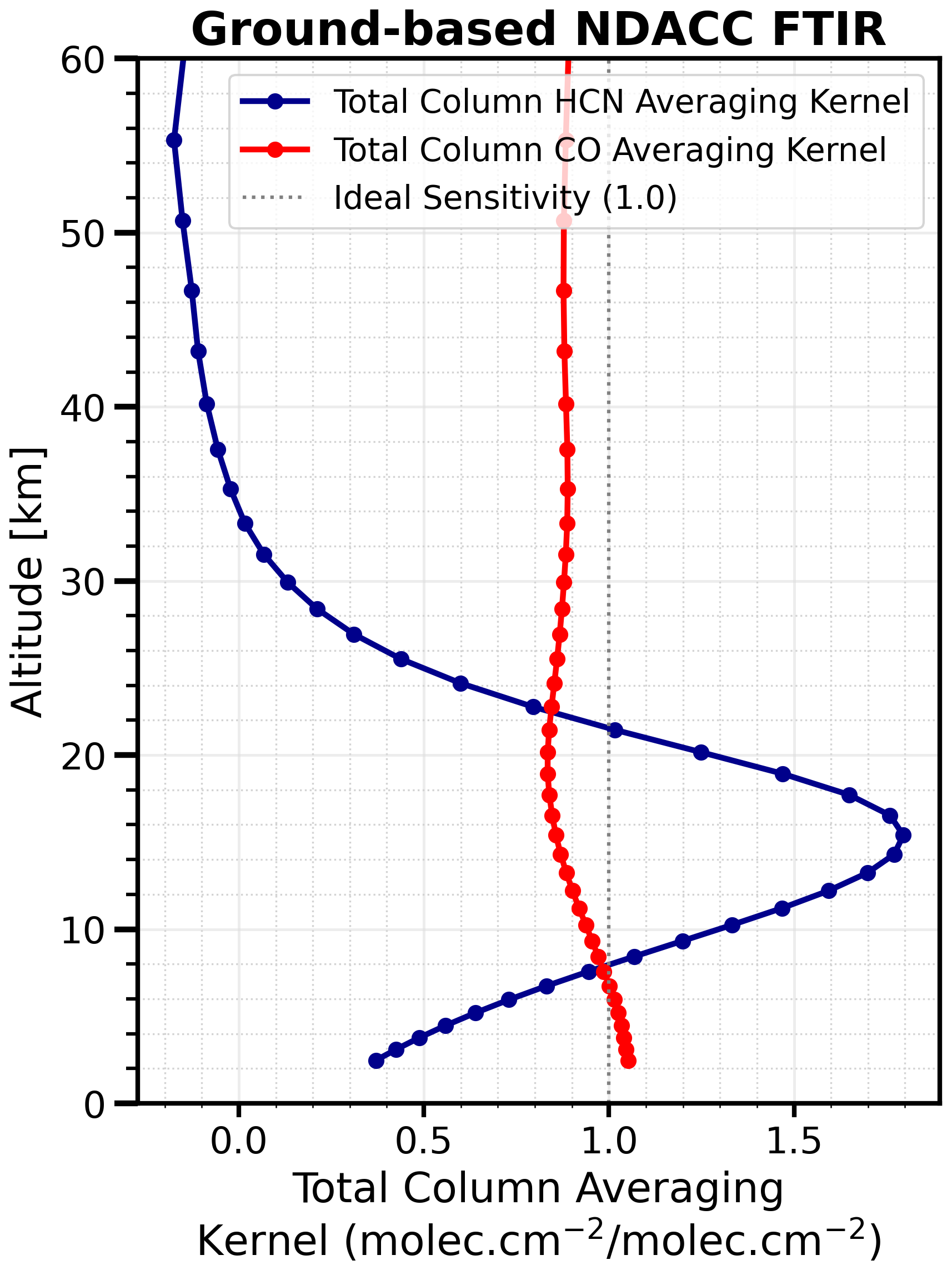
Figure 2 Average total column averaging kernels for ground-based FTIR at Reunion Maido for CO (red line) and HCN (blue line) for measurements made in 2015.

Figure 3 shows the comparison between IASI and the ground-based measurements. Overall, the IASI observations closely agree with the ground-based FTIR CO measurements. For the 2013–2019 period where FTIR data were available to use, the IASI columns are only biased high by 0.7 % ± 4.4 %, where the uncertainty represents the 1-sigma standard deviation on the mean difference. The seasonality of CO is captured well in both datasets (correlation coefficient of 0.97 for the entire daily mean data set) with the peak CO in October and November periods each year, related to the Southern Hemisphere biomass burning season (Vigouroux et al., 2012). The maximum CO observed by IASI was 2.64 ± 0.052 × 10¹⁸ molec. cm⁻² in 2015; the peak FTIR value was 2.71 ± 0.054 × 10¹⁸ molec. cm⁻² in the same year, both instances occurring on 25 November 2015. For HCN at Reunion Maido, the IASI seasonality and interannual variability matches very well with the ground-based measurements (correlation coefficient 0.80 for the entire daily mean data set), but with IASI columns biased high by 14.3 % ± 7.0 %. This bias could be caused by a lack of consistency between the HCN spectroscopic line parameters in HITRAN used for the two retrieval schemes. Unlike the ULIRS HCN retrieval, the NDACC retrieval uses the stronger HCN band near 3 micron. The maximum IASI HCN observed in 2015 of 1.66 ±  0.059 × 10¹⁶ molec. cm⁻² is 10.5 % higher than the highest HCN values observed in other years during the validation period. Compared to CO, the maximum HCN in 2015 occurred on 18 November, 2015. The CO total columns did not show a high discrepancy between different years in the record.

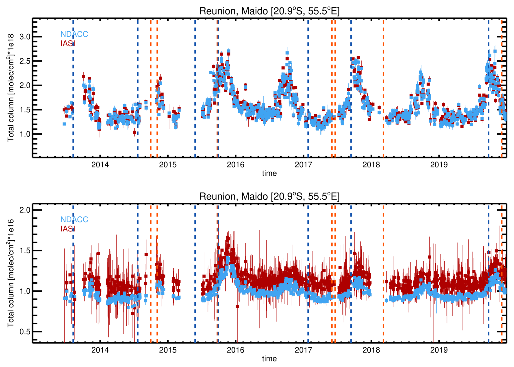
Figure 3 Time series of CO (top panel) and HCN (bottom panel) measurements for Reunion Maido. IASI measurements are shown in red with associated standard deviations (red lines). Ground-based FTIR measurements are shown in light blue with associated total error. The vertical blue (orange) dashed line represents where the IASI L2 (L1C) data processor version changed.

3.2 HCN emissions during the 2015 Indonesian fire season

3.2.1 Satellite observations of HCN in 2015

IASI satellite observations are used to estimate the amount of HCN emitted from the Indonesian region during the 2015 wildfire season; the plume of HCN emitted during the wildfire season is clearly visible in the left panel of Fig. 4. In Sect. 3.3, these observations are compared with those from the more recent 2019 and 2023 burning seasons, both of which also occurred under El Niño conditions.

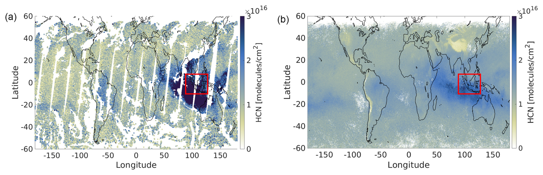
Figure 4 IASI global distribution of HCN total column (molec. cm⁻²) as retrieved by ULIRS for (a) 2 November 2015 during daytime and (b) the November 2015 monthly mean regridded on a 0.25° × 0.25° grid. The red box indicates the region (12° S–7° N, 90° E–127° E) over which the total column values are averaged.

According to the new peatland fire stages classification – stage 1 surface fire, stage 2 shallow peatland fire (depth < 20 cm) and stage 3 deep peatland fire (depth > 20 cm) – proposed by Hayasaka et al. (2020), the Indonesian fires of 2015 were classified as stage 2 for the second half of August and stage 3 from early September to the end of October. This is broadly consistent with the averaged total column of the IASI HCN observations seen in Fig. 5, where the highest HCN total columns are observed in September and October. The HCN total columns peak in late October/early November, consistent with the work of Nechita-Banda et al. (2018) on CO emissions from the same peat fires. Their results indicate a sudden increase in CO emissions for the latter half of October 2015.

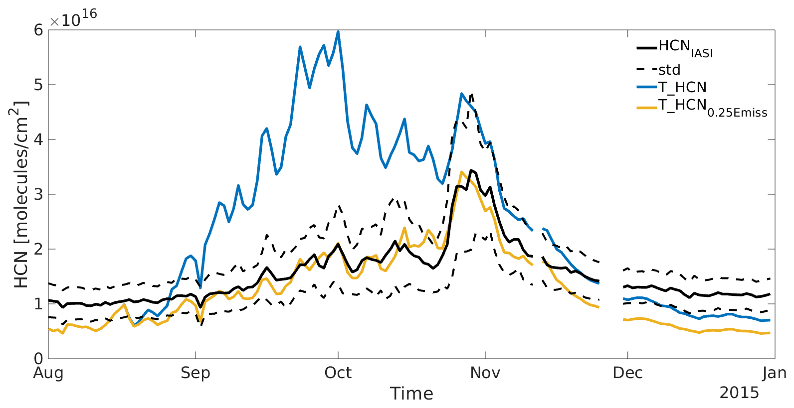
Figure 5 Comparison of the IASI measured HCN averaged total column time series (molec. cm⁻²) (black line), and HCN TOMCAT model run (T_HCN) using (i) monthly emissions from GFED v4.1 (blue line) and (ii) GFED v4.1 emissions with September values scaled to 25 % (orange line). The errors are defined as the standard deviation of the averaged total columns over Indonesia within the region 12° S–7° N and 90° E–127° E.

During neutral conditions, Indonesia is situated under one of the rising branches of the Walker circulation, linked to high rainfall. However, during El Niño, the circulation shifts eastwards and the air over Indonesia tends to sink, resulting in below average rainfall, higher surface pressure, and dryness. A plot of vertical winds at 0° latitude (Indonesia spans 95° E–140° E longitude) derived from ERA5 for October 2015 (Fig. 6) demonstrates this; the air mass over Indonesia is primarily descending. At the end of October/beginning of November, the circulation pattern suddenly changes to one in which the air is predominantly being uplifted. This is clearly observed in the top panels of Fig. 6, which shows the monthly mean ERA5 vertical wind vectors averaged along the equator for October 2015 and November 2015. The end result is that in late October, HCN from the peat fires is more readily uplifted to higher altitudes, coinciding with the region of the atmosphere where the IASI sensitivity is greatest, in the upper troposphere between 8 and 12 km. In addition to the increased emissions at the end of October, this contributes to the plume appearing most prominent in the first days of November 2015. The end of October 2015 also coincides with the onset of increased precipitation and an increase in soil moisture. Figure 7a shows that Indonesian deep soil moisture (SWI at the lowest layer corresponding to the characteristic timelength T=100, described in Sect. 2.3.2) for August–October 2015 was at its lowest level over the last decade, with a minimum at the end of October. The choice of the parameter T=100, the lowest layer of SWI, allows us to evaluate the water availability at the plant root depth. This strongly suggests that the GWL during the 2015 El Niño season was at a lower level than in any other year over the last decade. Precipitation for the same period was at the lower end of typical values for the given months as shown in Fig. 7b using IMERG data.

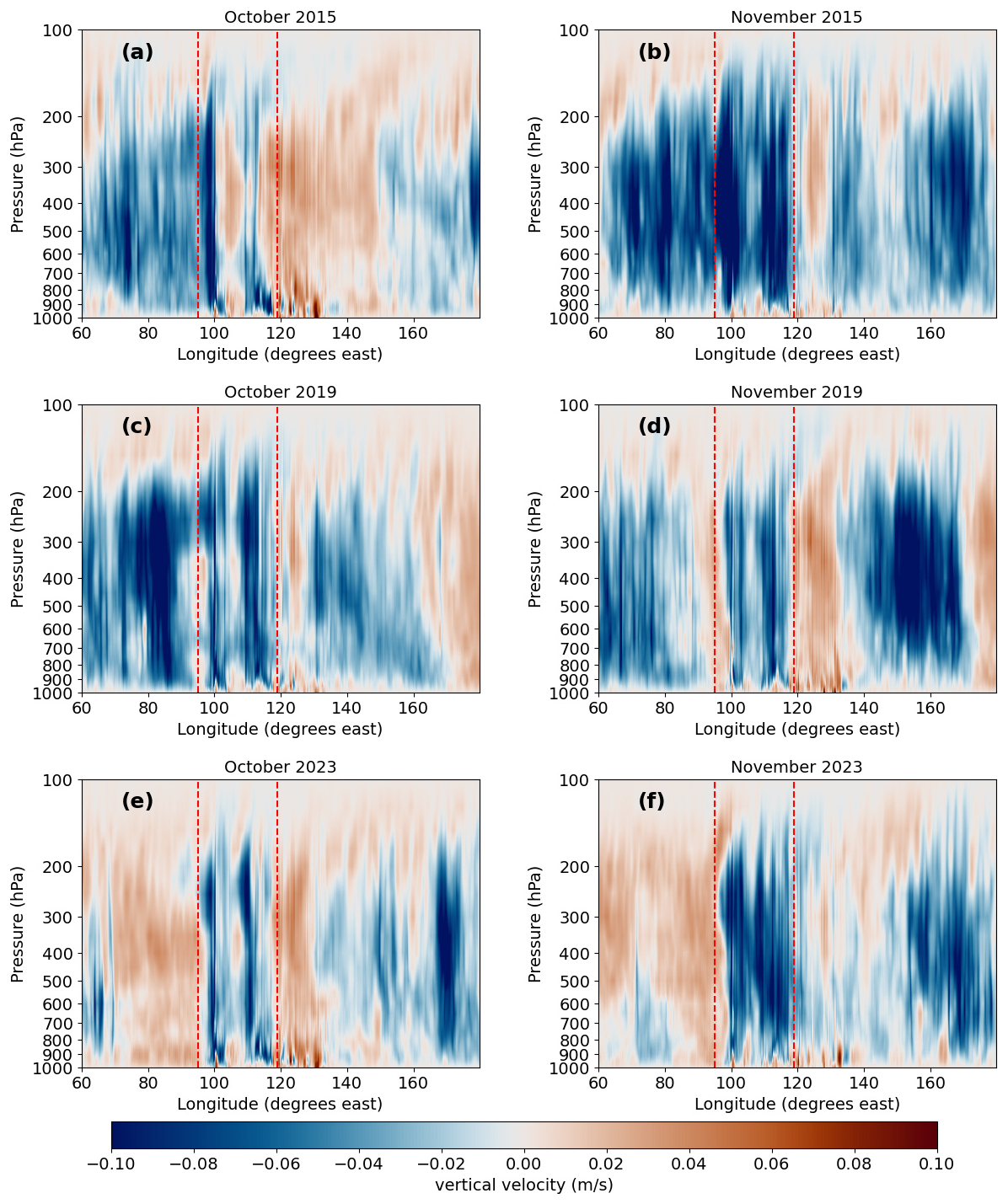
Figure 6 Monthly mean ERA5 vertical wind vectors (m s⁻¹) averaged along the equator for (a) October 2015, (b) November 2015, (c) October 2019, (d) November 2019, (e) October 2023, and (f) November 2023 (Hersbach et al., 2023). Brown (blue) areas indicate where, on average, the air is descending (ascending) for that particular month. The red dashed lines highlight the approximate meridional extent of the Sumatra and Kalimantan regions.

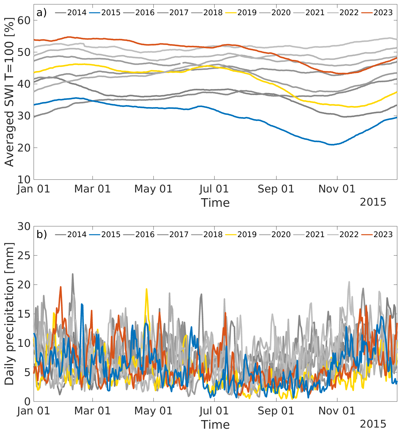
Figure 7 (a) Averaged SWI T=100, over Indonesia in the period 2014–2023. (b) Daily accumulated precipitation (combined microwave-IR) averaged over Indonesia estimate from the Integrated Multi-satellitE Retrievals for GPM (IMERG) in the period 2014–2023.

3.2.2 Evaluation of 2015 Indonesian HCN emissions using TOMCAT model simulations

In order to estimate the HCN emissions from the 2015 Indonesian peat fires, retrieved HCN total columns from IASI are compared with outputs of a tracer version of the TOMCAT 3D CTM.

Figure 5 compares the averaged total column time series of HCN, calculated over Indonesia in the regional box [12° S–7° N, 90° E–127° E] for both IASI measurements (black line) and the TOMCAT model outputs smoothed using the IASI averaging kernels (blue line). The box size was defined to cover Indonesia and, at the same time, capture the wildfire emission plumes. The IASI time series exhibits two gaps in November 2015 due to missing measurements. These same gaps also appear in the model time series, as the absence of IASI averaging kernels during this period prevents the smoothing of the model outputs. The T_HCN model run does not compare very well with the IASI measurements, showing a large overestimation of the HCN amount during the period between September and November 2015. In particular, the large peak simulated for T_HCN during the last week of September is completely absent from the IASI measurements. The left panel of Fig. 8 shows the HCN total column distribution on 2 November 2015 produced from T_HCN. The HCN amount produced is globally overestimated compared with the IASI measurements reported in Fig. 4, in particular over the latitude band between 20° N and 40° S. The discrepancy observed between the HCN TOMCAT model and IASI measurements is seemingly caused by the HCN emissions used to drive the model, shown in Fig. 9, which combine GFED v4.1 (the main component), CMIP6 and CCMI as described in Bruno et al. (2023). These emissions indicate an anomalously large peak of more than 4×10¹¹ molec. cm⁻² s⁻¹ in September 2015. This value is more than double the October emissions, during which the largest HCN concentrations were observed over Indonesia during the 2015 wildfire season.

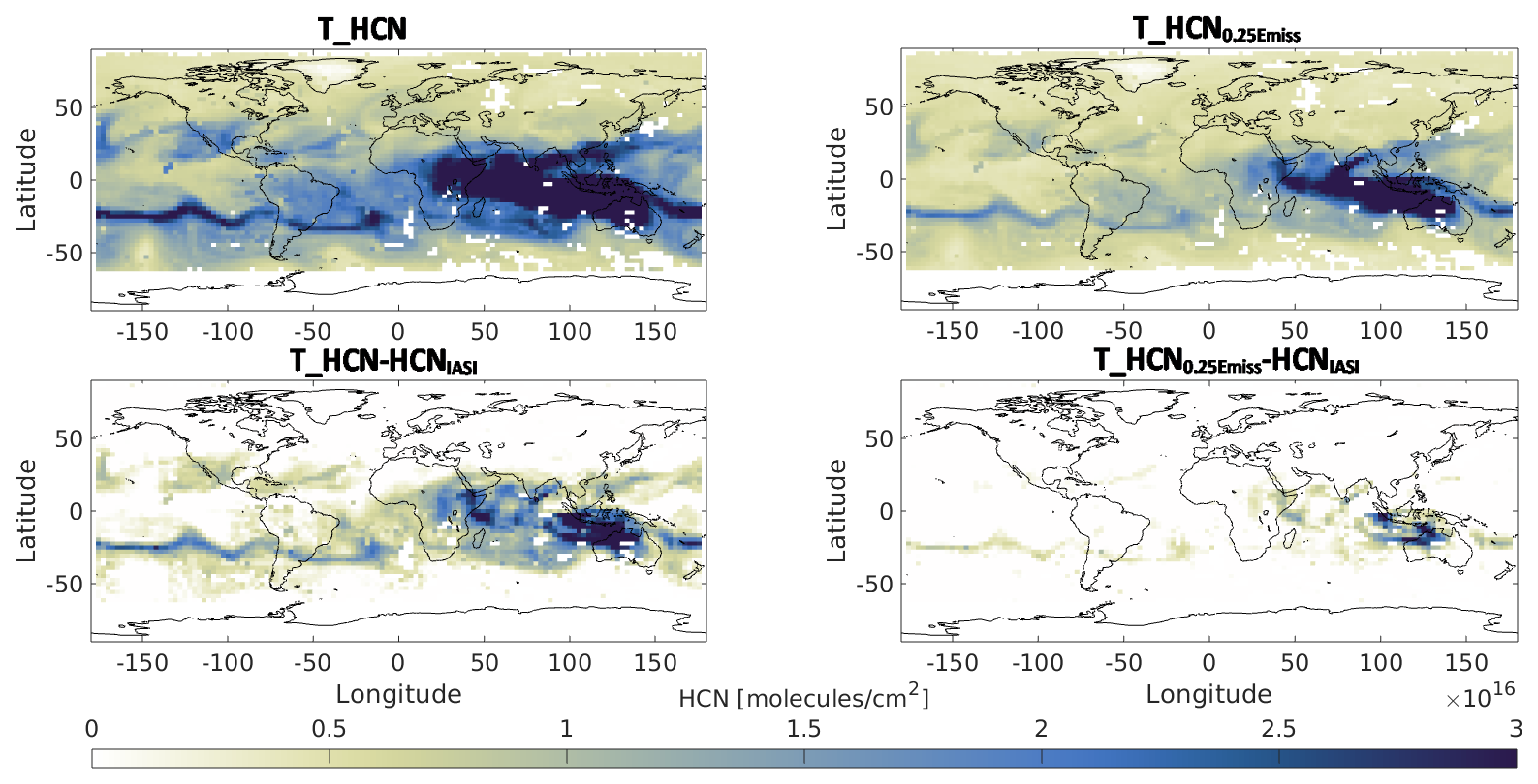
Figure 8 Global distribution of HCN total column (molec. cm⁻²) on 2 November 2015 produced from (a) T_HCN and (b) T_HCN_0.25Emiss. The bottom panels shows the total column difference between the two runs and the IASI measurements regridded on the TOMCAT grid.

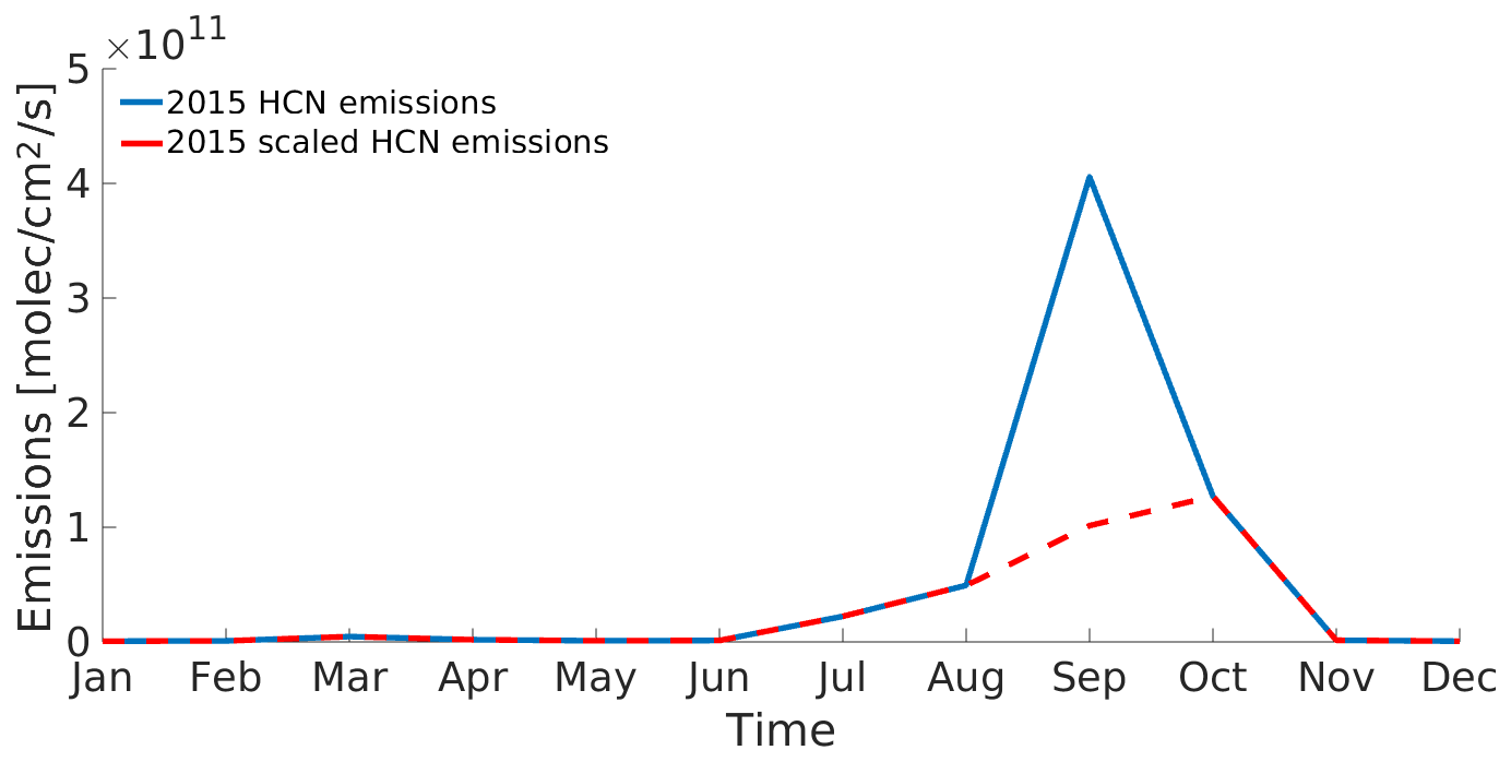
Figure 9 Monthly average HCN 2015 emissions (molec. cm⁻² s⁻¹) used in the T_HCN TOMCAT model experiment (blue line) compared with the scaled emissions used in the T_HCN_0.25Emiss experiment (red dashed line).

In order to seek better agreement between model and observations, we performed a number of model sensitivity runs. These suggested that the most sensitive component for improving the model simulations was the September GFED HCN emissions. For this reason, a new model run was performed (T_HCN_0.25Emiss) in which the September 2015 emissions were reduced by 75 %, based on the analysis performed in Bruno (2024b). The orange line in Fig. 5 indicates the averaged total column (smoothed by the IASI HCN averaging kernels) over Indonesia for the T_HCN_0.25Emiss model run, showing a substantial reduction in HCN concentration during September and October and reaching a very good agreement with the IASI measurements. However, the background HCN values, e.g. in December, are underestimated in the model, possibly due to neglect of additional sources. The global HCN total column distribution modelled on 2 November 2015, as shown in the bottom right panel of Fig. 8, shows a significantly improved agreement with the IASI measured HCN total columns in Fig. 4.

The study of CO emissions from the 2015 Indonesian wildfire season by Nechita-Banda et al. (2018) found that GFED is not good at reproducing emissions from large peat fires. GFED estimates monthly fire emissions from satellite-observed burned area and temporally disaggregates them within each month using fire radiative power as a proxy for combustion intensity and timing. For peat-dominated fires, burned area is more sensitive to the initial burning stages and less sensitive to peat burning that occurs underground. Our work supports this conclusion with respect to emissions of HCN from peat fires.

3.2.3 Enhancement ratios and emission factors

The Indonesian peatland fires from 2015 present an opportunity to estimate the HCN wildfire emission factors from satellite data. The fires burned for several months over a limited area, with the prevailing wind conditions resulting in the emitted plumes being predominantly transported over the Indian Ocean. The relatively long lifetimes of HCN and CO, of the order of 2-5 months, allow us to take advantage of satellite measurements over the ocean, where surface emissivity is reasonably homogeneous, and where the polluted air has been uplifted to higher altitudes, corresponding to the maximum sensitivity of IASI to HCN and CO perturbations. Changes in thermal heating over land between day and night cause a change in vertical sensitivity of IASI to HCN and CO. The effect over the oceans is much smaller due to the larger heat capacity of water. As such, in this work we use an average from both IASI daytime and night time measurements to maximise coverage and reduce the random uncertainty of the results.

The emission factor (EF_X) is a quantity defined as the mass of a trace gas (X) emitted per kilogram of biomass burned (g kg ⁻¹ dry matter). In order to derive EF_X, it is first necessary to derive a related parameter called the enhancement ratio (ER) which can be determined directly from satellite measurements. The ER${}_{\mathrm{HCN}/\mathrm{CO}}$ is defined as a ratio of the emitted number of molecules of HCN over the emitted number of molecules of CO (Goode et al., 2000; Whitburn et al., 2017),

$$\begin{array}{}\text{(2)}& {\mathrm{ER}}_{\mathrm{HCN}/\mathrm{CO}}={\displaystyle \frac{[\mathrm{HCN}{]}_{\mathrm{plume}}-[\mathrm{HCN}{]}_{\mathrm{background}}}{[\mathrm{CO}{]}_{\mathrm{plume}}-[\mathrm{CO}{]}_{\mathrm{background}}}}\end{array}$$

CO is chosen as the reference gas in this work as it has a similar lifetime to HCN and is emitted from similar sources. The excellent daily coverage of IASI allows a daily estimation of ER${}_{\mathrm{HCN}/\mathrm{CO}}$ to be performed. We have chosen the region 12° S–7° N, 90° E–127° E, located downwind of the Indonesian emissions from Sumatra and Kalimantan; only data with a correlation coefficient greater than 0.3 (following threshold methodology of Whitburn et al., 2017) are included in our analysis. There is no clear trend in the ER across the September 2015 to December 2015 period (Fig. 10), although there is some variability with lower ER in early September, where the correlation between HCN and CO measurements is less than 0.4. The phase of fire is a key factor in the emission of pyrogenic species. HCN and CO emissions are generally higher during the smouldering phase of fire (lower FRP) with smouldering peat fire emission factors being approximately 10 times those of flaming savanna fires (Hu et al., 2018). Peat fires generate weakly buoyant smoke plumes (Hu et al., 2019) that generally accumulate close to the ground, although the emissions can migrate great distances via the prevailing winds. The lower ER in early September may be due to the fact that the fires were only recently ignited and high HCN (and CO) levels were closer to the ground. IASI is more sensitive to near surface CO than HCN, so HCN is likely underestimated at that time. Throughout October, the HCN : CO relationship shows correlation coefficients greater than 0.4. By early November, the fire activity ended abruptly, but the correlation remains greater than 0.3 throughout most of November, until the HCN levels drop below the sensitivity of the IASI instrument.

It is estimated that 90 % of fire emissions from the late 2015 fire events were dominated by emissions from peat soils (Whitburn et al., 2017), with the remaining 10 % from tropical forest. Using a range of ERs derived for differing correlation coefficients, we are able to estimate HCN emission factors, EF${}_{\mathrm{HCN}/\mathrm{CO}}$, from the derived ER${}_{\mathrm{HCN}/\mathrm{CO}}$. Since we are investigating a region close to the emissions, and are not influenced by transport from other regions, the two parameters are related by the equation

$$\begin{array}{}\text{(3)}& {\mathrm{EF}}_{\mathrm{HCN}}={\mathrm{ER}}_{\mathrm{HCN}/\mathrm{CO}}\times {\displaystyle \frac{{\mathrm{MM}}_{\mathrm{HCN}}}{{\mathrm{MM}}_{\mathrm{CO}}}}\times {\mathrm{EF}}_{\mathrm{CO}}.\end{array}$$

The quantities MM_HCN (27.0253 g mol⁻¹) and MM_CO (28.01 g mol⁻¹) are the molar masses of HCN and CO, respectively. There are a number of datasets of EF_CO for peat over Indonesia (Table 1). Stockwell et al. (2016) measured EF_CO in situ (291 ± 49 g kg⁻¹), noting that their measurements were solely from smouldering combustion. Huijnen et al. (2016) also measured EF_CO in situ (255 ± 39), but noted a few smoke measurements involved occasional contributions from small clumps of ignited dry vegetation, which may account for the smaller value of EF_CO. More recently, Yokelson et al. (2022) revisited Kalimantan in 2019, during El Niño conditions, to sample fires burning only peat and measured a 50 % larger EF_CO compared to the Stockwell et al. (2016) work in a similar region. Both Christian et al. (2003) and Stockwell et al. (2016) took samples from Sumatra and Kalimantan respectively and burned the samples in the lab, both deriving significantly lower EF_CO values. The final source is from a meta-analyses study by Rodriguez Vasquez et al. (2021) who use the data from the in situ and laboratory studies previously listed to derive an updated EF_CO based on methodological differences in measurements and weighted to account for different sample sizes.

Yokelson et al. (2022)Rodriguez Vasquez et al. (2021)Stockwell et al. (2016)Huijnen et al. (2016)Stockwell et al. (2014)Christian et al. (2003)

Table 1 Derived emission factors, EF_HCN, in g kg⁻¹ dry Matter. EF_HCN has been calculated via Eq. (3) by using a number of EF_CO values from the literature. EF_HCN is then calculated for all of the ER results presented in Fig. 10 over the region [12° S–7° N, 90° E–127° E]. Note that “n/a” denotes not applicable.

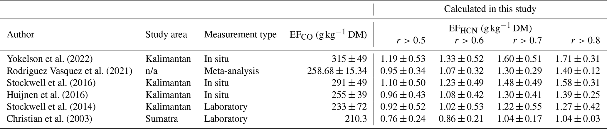
Examining the relationship between HCN and CO total column amounts in Fig. 10, the correlation coefficient between the two species varies between 0.3 and 0.8 over most of the September to November 2015 period. We use the correlation coefficient as a filtering metric here to understand whether we see a change in the ER depending on how closely related CO and HCN concentrations are in the same air parcel. A summary of the effect on estimating EF_HCN by including only measured data exceeding a chosen correlation coefficient threshold is shown in Table 1. Generally, the lower correlation coefficients are found to be associated with lower ER values. The highest EF_HCN values are derived where the correlation coefficient exceeds 0.8, ranging between 1.04 and 1.71 g kg⁻¹ depending on which value is used for EF_CO. Where the correlation coefficient HCN:CO is greater than 0.5, we see that the EF_HCN estimates decrease, ranging between 0.76 and 1.19 g kg⁻¹. Both ends of the estimates are lower than the (surface) in situ and lab-based estimates of EF_HCN. We know that the IASI HCN sensitivity is in the upper troposphere between 8 and 12 km, with very low sensitivity to high concentrations below 4 km which may lead to an underestimate of EF_HCN. Field et al. (2016) show that the MLS CO at 215 hPa (∼ 12 km) increased steadily through September with a rapid increase to CO exceeding 400 ppbv at the end of October. The highest correlation HCN : CO in our results is during this late October period, where we see enhanced vertical uplift of both gases and therefore increased sensitivity to the HCN emissions. Before mid-October, we likely underestimate the HCN amounts as plumes are closer to the surface. This alone cannot explain the large discrepancies between the IASI measurements and the TOMCAT simulations observed in Fig. 5, since the TOMCAT outputs have already been smoothed using the IASI averaging kernels to ensure comparable sensitivity.

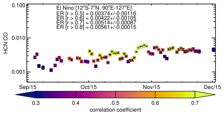
Figure 10 Daily HCN enhancement ratios (ER) relative to CO calculated from the slope of the linear regression of HCN against CO total columns between 1 September and 1 December 2015, over the Indian Ocean (12° S–7° N, 90° E–127° E). For completeness the error bars, although small, are included and correspond to the standard errors on the regression slope. Any data with a correlation coefficient < 0.3 for the slope have been excluded.

3.3 Comparison of the 2015 Indonesian fire season with 2019 and 2023

According to the ONI, the 2015 El Niño event was one of the strongest in the satellite era. ONI is the primary index used by NOAA to monitor and classify El Niño and La Niña events (NOAA Climate.gov, 2009). Defined as a running 3-month mean sea-surface-temperature anomaly for the Niño 3.4 region (5° N–5° S, 120°–170° W), El Niño events are defined as 5 consecutive overlapping 3-month periods above +0.5°. Figure 11 shows a plot of ONI as a function of time since 1990. It indicates that the recent 2023 burning season in Indonesia, also occurring during an El Niño event, peaked at the third strongest ONI value since 1990, behind only the 1997 and 2015 events. The 2019 event was comparatively weak.

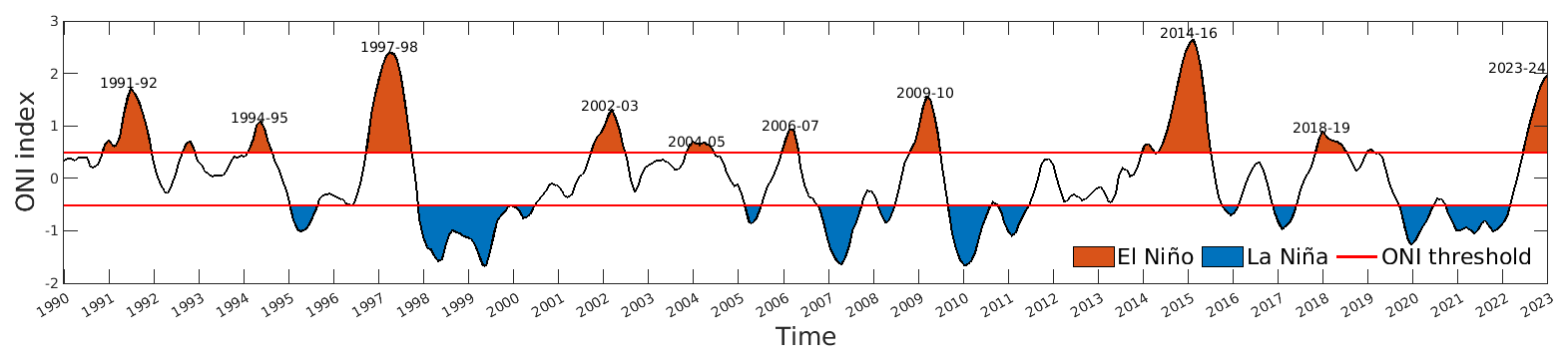
Figure 11 Time series from 1990–2023 of ONI index, with warm (red shaded area) and cold (blue shaded area) periods based on a threshold of ±0.5 °C.

In order to compare fire activity in Indonesia during the last three El Niño events, in late 2015, 2019 and 2023, we selected the VNP14IMG fire product across the whole 2012 to 2023 period and looked at the total fire activity across all of the Indonesian islands. Cumulative monthly fire radiative power over Indonesia is plotted in Fig. 12, and indicates that even during a notably strong El Niño phase, the fire activity in 2023 was almost eight times less than in 2015. Specifically in 2023 the fire activity was below the seasonal 2012–2023 average across the whole July–December period. For 2019, we observe significant fires in mid-September and a comparable increase in fire power to 2015 between early September and late September. From late September 2019, the fire activity abruptly ends, whereas 2015 maintains a steady increase in fire cumulative power until an abrupt end in fire activity in late October 2015.

We can use the ULIRS HCN to further investigate the emissions from the Indonesian peat fires. Figure 13 represents a 3 d simple moving average total burden HCN (in Gg) and CO (in Tg) for the three El Niño years. The total mass was calculated over the region 12° S–7° N, 90° E–127° E following Eq. (2) of R'Honi et al. (2013), and shows the highest values are towards the end of October 2015 for both gases. Comparing all three years used in this study, we see the highest HCN values across the September to November period always occur in 2015. The HCN concentrations increase in early September 2015 and are shown to be coincident with an increase in fire activity during the same period (Fig. 12), rapidly exceeding 500 Gg by 25 September. After this period we see the largest increase in HCN between 22 October and 30 October, to approximately 600 Gg of HCN, peaking at 1056 Gg on 29 October. This increase can also be linked to increasing fire power over that period, although we note that the increase in fire power is also conducive to extra lofting of the elevated HCN to altitudes where the IASI instrument is more sensitive to HCN changes (i.e. the upper troposphere). After 1 November, concentrations of HCN decrease for the remainder of 2015. For 2019, the pattern in early September mirrors that in 2015 with a sudden increase of 240 Gg of HCN between 3 September and 26 September. After that, HCN concentrations decrease back to the 300 Gg baseline by 9 October and stay at these lower levels for the rest of 2019. In 2023, we observe no significant enhancements in HCN across the August to December period, relative to the 300 Gg baseline. For CO in 2015 there is a gradual increase in total CO from early September with a peak of 168 Tg in late October, similar to HCN. Throughout November the CO burden decreases and is back at background levels by early December. In 2019, the CO shows a similar variability to HCN, increasing through September but decreasing again in October 2019.

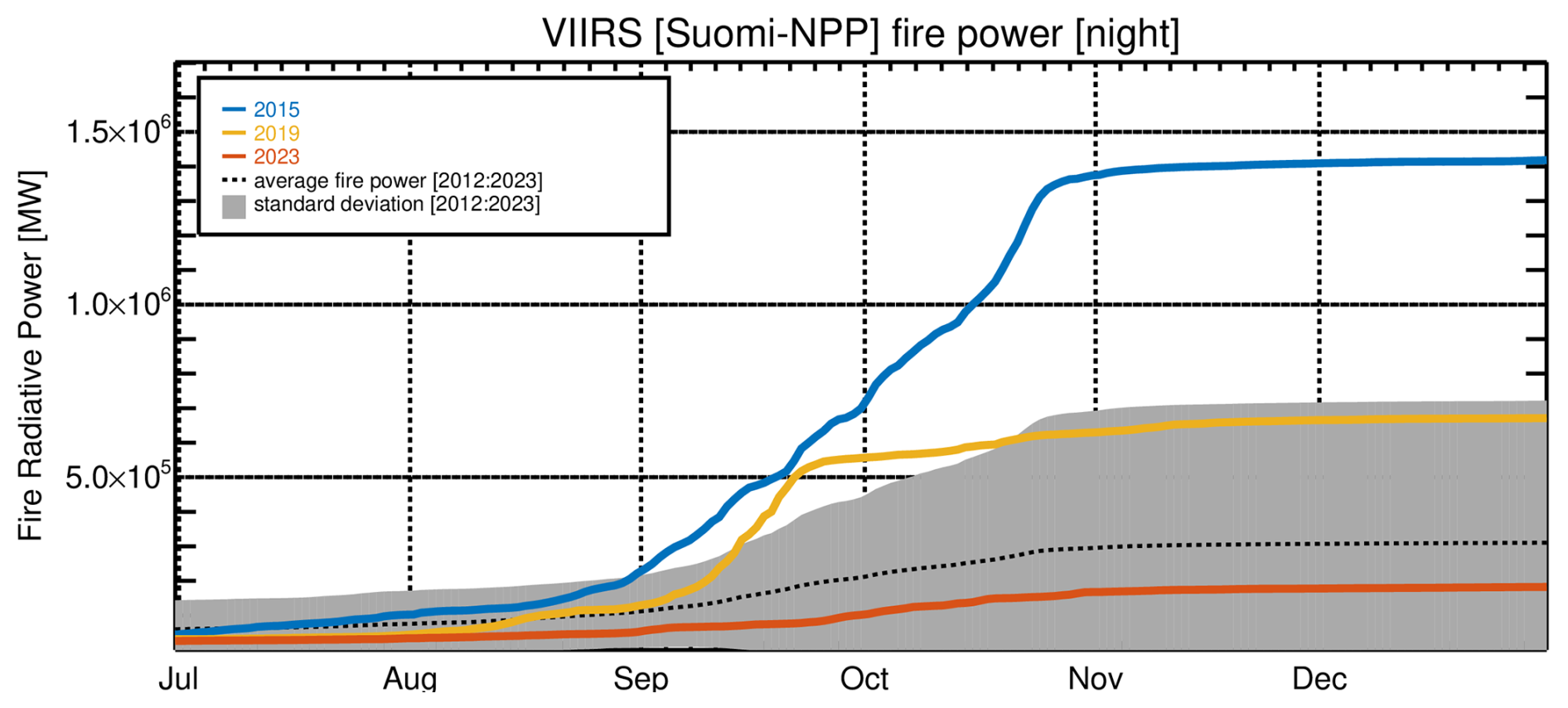
Figure 12 Total cumulative monthly fire radiative power (MW) over Indonesia measured by VIIRS. The fire activity in 2023 (red line) is almost eight times smaller than in 2015 (blue line), and falls below the seasonal long-term (2012–2023) mean (black dotted line).

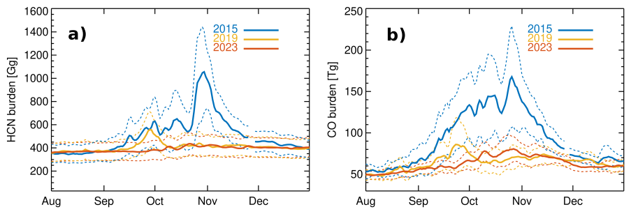
Figure 13 Daily Infrared Atmospheric Sounding Interferometer (IASI) derived (a) HCN burden (Gg) and (b) CO burden (Tg) between 1 August and 31 December for three years: 2015 (blue line), 2019 (yellow line), and 2023 (red line). This is calculated for the region 12° S–7° N, 90° E–127° E.

Comparing the circulation patterns across the equator in October 2015 and 2023 in Fig. 6, it is clear that the regimes are quite different, with the descending air over Indonesia in 2015 replaced by more neutral conditions in October 2023. These conditions are less conducive to prolonged dry periods, which would allow peat fires to establish if left unchecked. Over the western Pacific Ocean itself, October 2023 showed much less wide-scale descent of air compared to 2015, suggesting that the Walker circulation did not weaken significantly in late 2023. The circulation patterns across the Eastern Indian Ocean (60° E–110° E) in October 2015 and October 2019 are remarkably consistent. Over Indonesia itself (100° E–120° E) the vertical winds exhibit very different behaviours between 2015 and 2019, with 2019 conditions more conductive to convection and increased rainfall, which would likely suppress fire activity.

Figure 7b indicates that the precipitation levels in August to October for the El Niño years 2015, 2019 and 2023 were very similar. However, Fig. 7a demonstrates that the SWI in the lowest soil layer towards the end of 2019 and 2023 was quite typical of values over the last decade, unlike 2015 which was significantly drier. This is consistent with previous work showing that peat moisture, in particular the GWL, is a major factor in determining the ignition and spread of peat fires (Hayasaka et al., 2020).

3.3.1 HCN emission database using the FINNpeatSM method

Peatland fire emissions from GFEDv4s include a simple representation of burn depth based on soil moisture. However, it is not possible to use the dataset to explore soil moisture and burn depth interactions across different years. Therefore limiting our ability to explore the drivers of differences in HCN retrievals between 2015, 2019 and 2023. To address this limitation in GFEDv4s, we examine fire detections (from VIIRS fire hotpots) and SMAP (ONeill et al., 2021) over Indonesia peatlands. Using the FINNpeatSM method (Kiely et al., 2019), we can combine these datasets to estimate the burn depth of fires in 2015, 2019 and 2023.

Daily VIIRS temperature hotspots are only used if there is a medium or high confidence in the retrieval (Wiedinmyer et al., 2011) and if the fire occurred on peatland in Indonesia. For each retained fire detection, the nearest-neighbour daily mean soil moisture pixel (from SMAP) is determined. The associated soil moisture from an individual fire detection can be used to estimate the burn depth, and emissions, of the fire. The emissions in FINNpeatSM are linearly related to burn depth, so that the deeper a fire burns the higher the emissions.

First, we consider daily mean soil moisture from SMAP across all Indonesian, Kalimantan, and Sumatra peatlands for 2015, 2019 and 2023 (Fig. 14). We consider Kalimantan and Sumatra peatlands in addition to all Indonesian peatlands since these regions dominate fire emissions. In 2015 62 % of total emissions were from Kalimantan and 33 % were from Sumatra (Kiely et al., 2019). Soil moisture is shown for 1 June to 31 December, with the dry season (1 August to 31 October) shaded in grey, since the dry season is when fires are most likely to occur. Across Indonesia and both Kalimantan and Sumatra soil moisture in 2015, 2019 and 2023 were similar from June–July (0.58–0.61 m³ m⁻³). However, from July to August, soil moisture across all regions in 2015 and 2019 begins to decrease rapidly (from 0.52–0.55 to 0.46–0.48 m³ m⁻³), while in 2023 soil moisture remains high (0.59 to 0.54 m³ m⁻³). From August to mid-September soil moisture continues to decrease across Indonesia, driven by reductions in soil moisture in Kalimantan in 2015 and 2019 (Indonesia from 0.46–0.48 to 0.36–0.39 m³ m⁻³ and Kalimatan from 0.39–0.44 to 0.27–0.29 m³ m⁻³). In contrast, over the same period in 2023, soil moisture remains high across Indonesia (decreasing from 0.54 to 0.50 m³ m⁻³), driven by high soil moisture in Sumatra peatlands. From mid-September to mid-October soil moisture continues to decrease in 2015 (from 0.39 to 0.33 m³ m⁻³), while in 2019 there is an abrupt increase in soil moisture (from 0.36 to 0.47 m³ m⁻³), closer to the 2023 values (from 0.50 to 0.54 m³ m⁻³). Overall, soil moisture is lowest throughout the dry season in 2015 (1 August to 31 October mean of 0.40 m³ m⁻³), while in 2019 soil moisture is very low at the start of the dry season but then increases in the late dry season (1 August to 31 October mean of 0.43 m³ m⁻³). In contrast, soil moisture in 2023 is the highest of the 3 years (1 August to 31 October mean of 0.52 m³ m⁻³), in agreement with what was observed in SWI data (Fig. 7a).

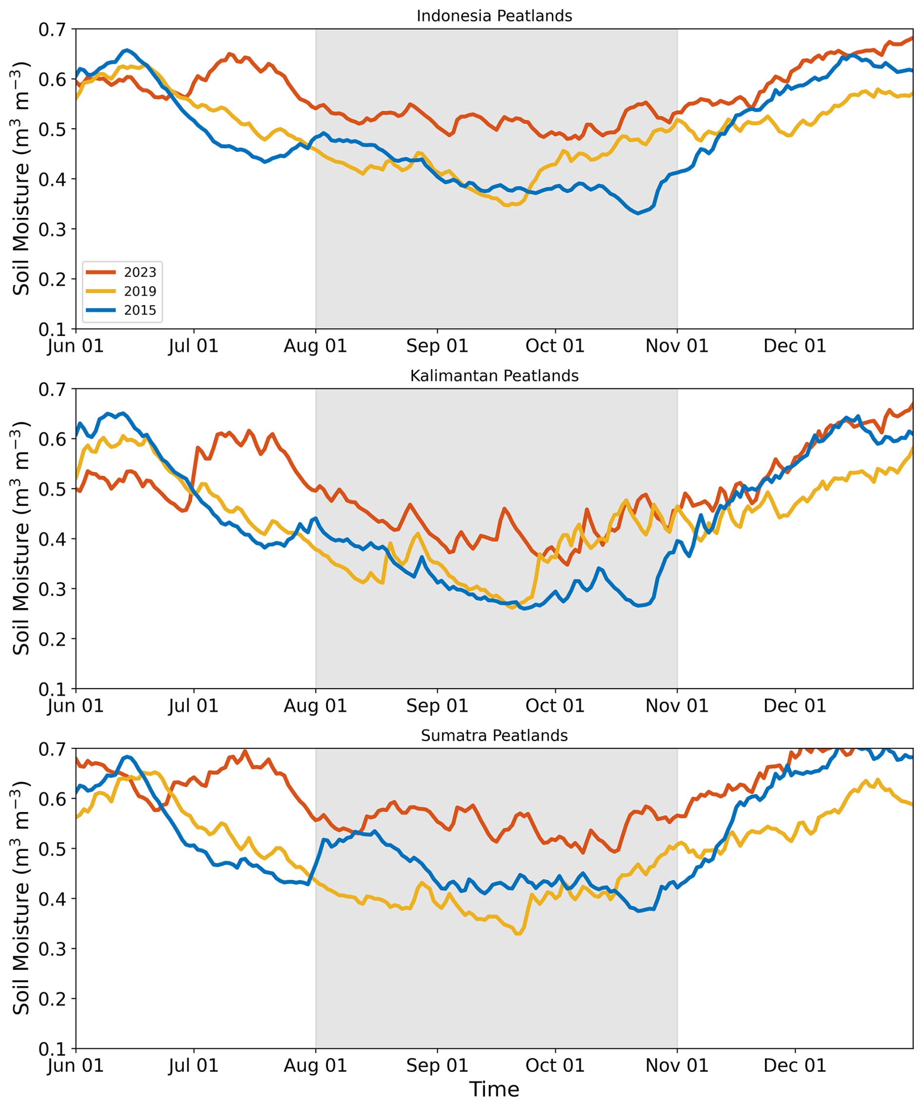
Figure 14 Timeseries of daily mean SMAP soil moisture (m³ m⁻³) for all Indonesian peatlands, Kalimantan peatlands and Sumatra peatlands for 2015 (blue), 2019 (yellow) and 2023 (red) for the period 1 June to 31 December in years 2015, 2019 and 2023.

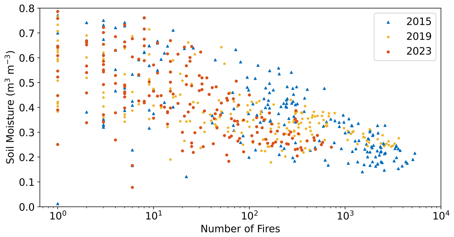
Figure 15 Daily Indonesian peatland fire count (from VIIRS) and collocated daily soil moisture (m³ m⁻³) for the period 1 June to 31 December in years 2015 (blue triangles), 2019 (yellow stars) and 2023 (red circles).

The collocated daily mean soil moisture and daily total number of fire hotspots (from VIIRS) for the same time period (1 June to 31 December 2015, 2019 and 2023) is shown in Fig. 15. This clearly indicates that 2015 had the highest number of fire hotspots (> 40 collocated pixels with 1000–10 000 fire hotspots) occurring in areas where soil moisture was low (0.15–0.35 m³ m⁻³). However, in 2019, there are fewer fire pixels with a high number of hotspots (24 pixels with 1000–10 000 fire hotspots) and they generally had higher soil moisture (0.25–0.31 m³ m⁻³). In 2023, there were both fewer pixels with a high number of fire hotspots (peaking at 100–1000 fire hotspots), and the soil moisture where fire hotspots occurred was higher (0.21–0.4 m³ m⁻³).

The soil moisture at each fire location can be used to calculate peat burn depth of the fire, using the method developed by Kiely et al. (2019). Figure 16 indicates the burn depth of fires, and the date they occurred. As shown in Fig. 15, 2015 has the highest number of fires (up to 25 000 fires) that occur in low soil moisture areas (0.3 m). Figure 16 indicates that these fires burn deep into the peat below (0.25–0.3 m) and occur between September and mid-October 2015 (in line with Fig. 14). In contrast, in 2019, there are fewer fires (0–15 000), the burn depth is shallower (0–0.25 m), and the fires that burn the deepest occur earlier in the dry season (mid-September) when soil moisture is higher than 2015 (Fig. 14). In 2023, far fewer fires (0–5000 fires) burn deep into the peat below (0.05–0.25 m) and deep burning occurs in mid-September to early-October, in line with increased soil moisture in 2023 (Fig. 14).

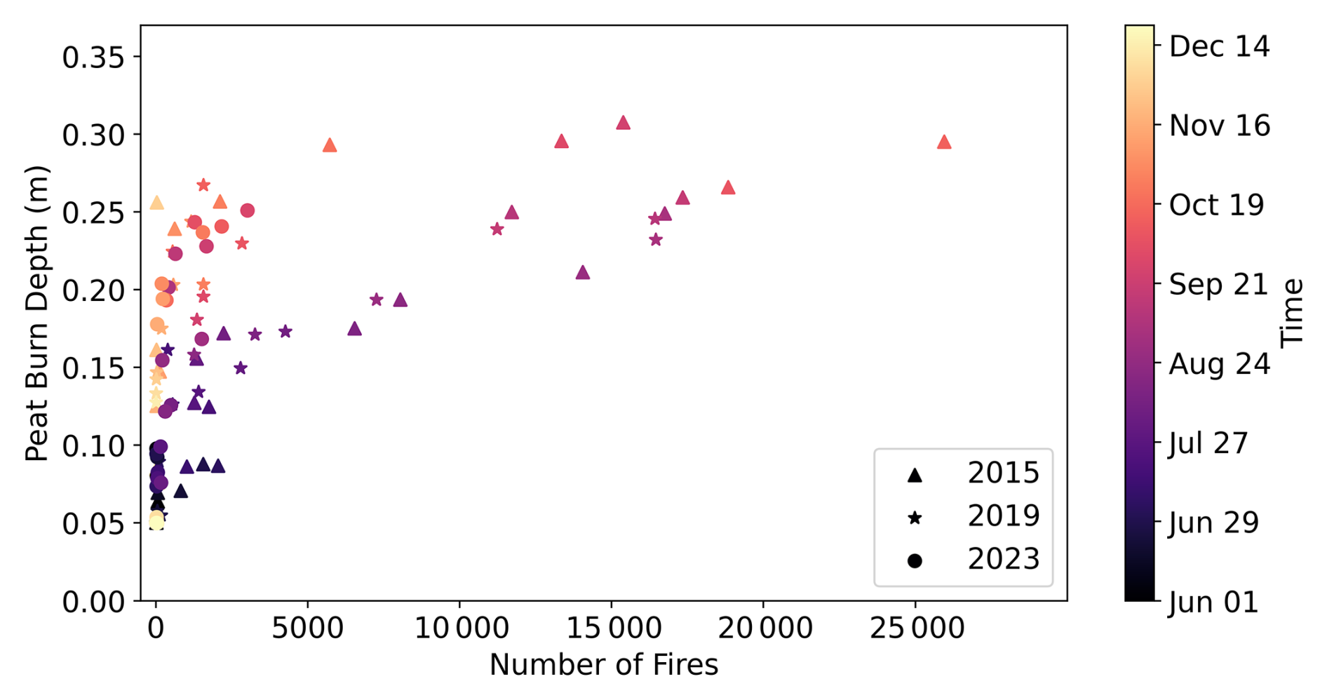
Figure 16 Weekly mean burn depth (m) of Indonesia peat fires between 1 June and 31 December in years 2015 (triangles), 2019 (stars) and 2023 (circles).

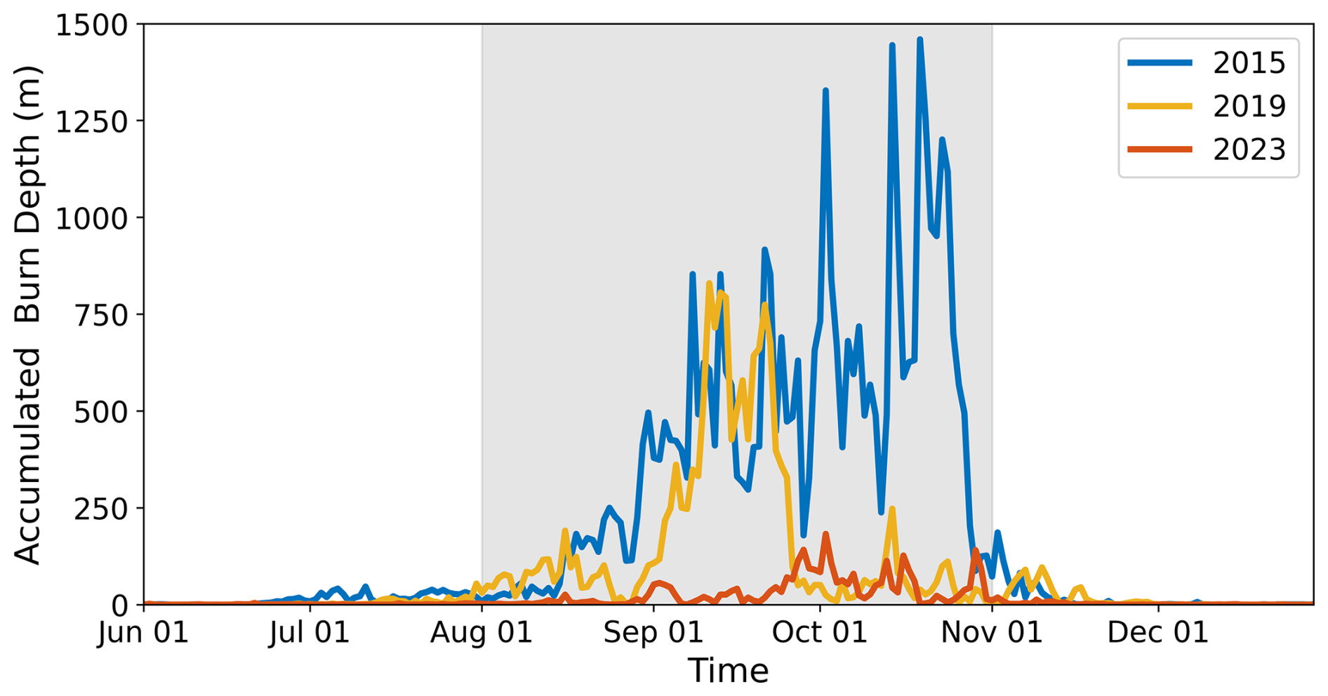
Figure 17 Accumulated daily burn depth of Indonesian peatland fires in 2015 (blue), 2019 (yellow) and 2023 (red) between 1 June and 31 December.

The accumulated daily burn depth of all Indonesian peatland fires from 1 June to 31 December is shown in Fig. 17. This plot accounts for both the number of fire hotspots and the burn depth of individual fire hotspots. At the start of the dry season (August to mid-September) the accumulated burn depth in 2015 and 2019 is similar (500–1000 m), compared with < 100 m in 2023. This is likely because soil moisture at the start of the dry season (August to mid-September) is similar in both years, and both years have a similar number of fire hotspots at this time. However, from mid-September, 2015 and 2019 deviate. Accumulated burn depth remains high in October 2015, whereas it substantially decreases in 2019. This is likely driven by the large decrease in both fire hotspots and peatland soil moisture in 2019, compared with 2015 where the number of fire hotspots remains high and the peatland soil moisture remains low.

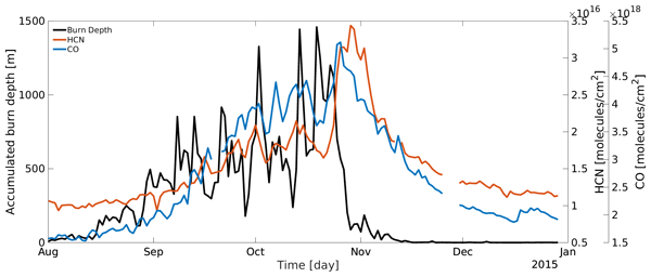
As illustrated in Fig. 18, the time series of accumulated daily burn depth, along with the averaged total column of HCN and CO, exhibit similar temporal patterns, a progressive increase from August through October, reaching a peak in late October, and subsequently declining sharply in November.

3.4 Temporal relationship between burn depth and HCN and CO total column during 2015 wildfires

The temporal relationship between two time series can be investigated using the cross-correlation function, which quantifies the linear association between two variables as a function of temporal lag (Storch and Zwiers, 1999). For two stationary time series x_t and y_t, the cross-correlation at a given lag k is defined as the normalized covariance between x_t and y_t−k:

$$\begin{array}{}\text{(4)}& {\mathit{\rho }}_{xy}\left(k\right)={\displaystyle \frac{\mathrm{cov}(x_t,y_{t-k})}{{\mathit{\sigma }}_x{\mathit{\sigma }}_y}},\end{array}$$

where σ_x and σ_y denote the standard deviations of the two series. In practice, the covariance is estimated from the sample values as

$$\begin{array}{}\text{(5)}& {\mathit{\rho }}_{xy}\left(k\right)={\displaystyle \frac{{\sum }_{t=\mathrm{1}}^{N-k}(x_t-\overline{x})(y_{t-k}-\overline{y})}{(N-k){\mathit{\sigma }}_x{\mathit{\sigma }}_y}},\end{array}$$

where $\overline{x}$ and $\overline{y}$ are the sample means and N is the length of the time series. The resulting function ρ_xy(k) ranges between −1 and 1 and describes the strength of the linear relationship between the two variables at different lags. Positive lags indicate that variations in x lead those in y, whereas negative lags indicate that variations in y precede those in x.

A cross-correlation analysis between the accumulated daily burn depth and the total column concentrations of CO and HCN can provide insights into the temporal dynamics of plume transport. As shown in Fig. 19, both HCN and CO exhibit maximum positive correlations with the burn depth at non-zero lag times, indicating that the fire activity at the surface anticipates the appearance of enhanced trace gas signals at the respective altitudes of high sensitivity of the IASI instrument. Specifically, the cross-correlation peaks at a lag of approximately −10 d for both species, suggesting that 10 d is the typical timescale required for emissions from peatland fires to be transported and mixed into the mid- to upper-tropospheric layers. The cross-correlation function (XCF) for HCN (black line) and CO (orange line) displays a broadly similar temporal structure, with both curves rising steadily from negative lag values, peaking near −10 d, and subsequently declining into negative correlation at higher lag values. The slightly larger peak for CO may reflect differences in vertical transport dynamics or sensitivity profiles, given that CO exhibits dual sensitivity in both the lower and upper troposphere, whereas HCN is primarily sensitive to the mid-troposphere (∼ 10–12 km), as described in Sect. 2.1.1. These results support the interpretation that the observed trace gas enhancements are closely linked to fire activity and that the lag time to maximum correlation can serve as an estimate of the average vertical and horizontal transport time of the emission plume.

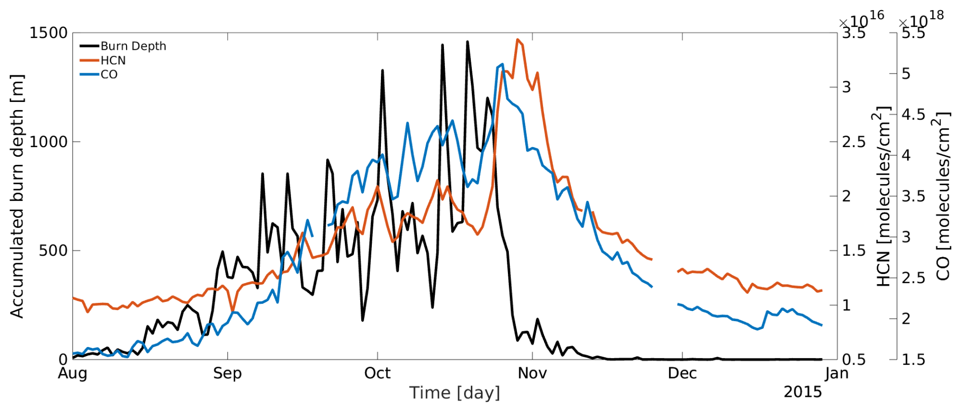
Figure 18 IASI measured HCN (red line) and CO (blue line) averaged total column and accumulated daily burn depth (black line) of all Indonesia peatland fires from 1 August to 31 December 2015.

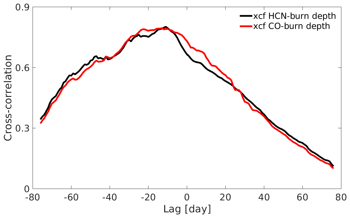
Figure 19 Cross-correlation between the IASI HCN total column and the accumulated daily burned depth (black line) and between the IASI CO total column and the accumulated daily burned depth (red line).

4 Conclusions

This study has provided a comprehensive assessment of Indonesian peatland fire emissions during recent El Niño events, with a particular focus on HCN as a tracer of smouldering combustion during peat fires. By integrating IASI satellite retrievals with TOMCAT model simulations, precipitation and soil moisture observations, and fire activity datasets, we have quantified both the magnitude and variability of HCN emissions and identified the key drivers underlying interannual differences. The ULIRS retrieval approach has shown encouraging performance in the present study, and has been validated using observations from the Réunion Maïdo Observatory, located within a region directly affected by the Indonesian fires. Future work will focus on evaluating the ULIRS retrievals using NDACC observations over additional regions and latitude bands in order to demonstrate the broader applicability and robustness of the satellite product over a wider range of atmospheric conditions. The results provide strong evidence that the magnitude of trace gas emissions from Indonesian peatlands is not governed solely by the strength of El Niño but instead arises from the interaction between large-scale ocean–atmosphere dynamics and local hydrological conditions. The 2015 El Niño event, one of the strongest in recent decades, produced exceptionally large atmospheric concentration of HCN and CO, reflecting a combination of extremely low soil moisture, depressed groundwater levels, and deep burn depths in peatlands. The resulting emissions were unprecedented in the observational record, with IASI retrievals showing marked enhancements that were sustained through October and November.

In contrast, the 2019 and 2023 El Niño events, despite also being associated with positive Oceanic Niño Index (ONI) anomalies, resulted in markedly lower HCN burdens related to higher ground water content and atmospheric dynamics that make intense peat fires less favourable. The 2023 event, in particular, occurred under atmospheric circulation regimes that did not sustain prolonged dryness, resulting in fire activity that was nearly an order of magnitude almost eight times weaker than in 2015.

Using IASI total column measurements we also derive new satellite-based emission factors (EFs) for HCN enhancement ratios with CO during the 2015 dry season. These values provide independent, observation-based constraints that can improve the representation of peat fire emissions in models and inventories.

Comparisons between IASI-derived HCN total columns and TOMCAT model simulations revealed that the standard GFEDv4-based emission inventory substantially overestimates HCN emissions from peat fires during the 2015 dry season, particularly in September. A revised model run, applying a 75 % reduction to September emissions, produced much better agreement with satellite observations. This finding is consistent with the work of Nechita-Banda et al. (2018), who showed that GFED performs poorly in reproducing emissions from large peat fires because it relies on satellite-observed burned area and uses fire radiative power to temporally disaggregate emissions. In peat-dominated environments, the burned area is more sensitive to the initial stages of combustion and fails to capture prolonged subsurface smouldering. Together, these results suggest that current fire emission inventories misrepresent peat fire dynamics and are not well suited to capturing the contribution of underground smouldering processes to trace gas release. The analysis also confirms that the new FINNpeatSM approach, which explicitly links burn depth to soil moisture, offers a more accurate description of the dynamics of peat fire emissions.

Hydrological conditions emerged as a dominant control on fire intensity and emissions across all three El Niño events. Soil moisture and groundwater level determine not only the susceptibility of peatlands to ignition but also the persistence of smouldering fires and the total mass of peat carbon released to the atmosphere. When soils are dried, the peat layer can ignite and burn deeply, releasing large quantities of HCN and CO that are transported into the mid- to upper- troposphere within about 10 d. Conversely, higher soil water content suppresses combustion depth and limits the emissions. The strong cross-correlation between accumulated burn depth and satellite-observed HCN and CO concentrations further supports the close coupling between hydrology, fire behavior, and wildfire emissions.

The comparison of 2015, 2019, and 2023 further highlights that fire intensity and trace gas burdens are not determined solely by the strength of El Niño events, but rather emerge from the importance of the local drought intensity, soil moisture deficits, and atmospheric circulation patterns. This underscores the critical role of groundwater and soil moisture in regulating peatland vulnerability to ignition, smouldering persistence, and total emissions. Our results therefore emphasize the need for next-generation emission inventories that explicitly account for soil moisture and groundwater dynamics to better reproduce the peatland fire dynamics. Integrating satellite-derived products of atmospheric composition (e.g. IASI) and soil hydrology (e.g., SMAP, ASCAT, SWI) offers a valuable constraint for emissions and predictions of future fire behaviour under changing climate conditions. Such integrated approaches can reduce uncertainties in global fire emission estimates, improve the representation of smouldering combustion in chemical transport models, and enhance the predictive capacity for El Niño-induced fires during the dry seasons across Indonesia peat-dominated ecosystems. These advances are essential for understanding the contribution of peatland fires to regional air quality, global atmospheric composition, and the carbon–climate feedback system.