Inefficient consumption of natural gas drives methane emissions from a megacity

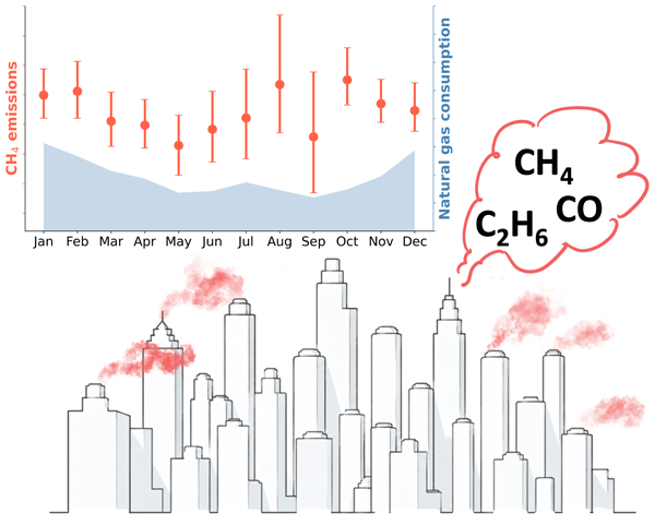
Reducing methane emissions offers a significant near-term opportunity for climate mitigation if the dominant sources are effectively targeted. Natural gas is a large and manageable methane source. Despite extensive pipeline upgrades in cities, methane reductions remain far smaller than expected, suggesting missing emission pathways. Using long-term tower observations in a U.S. megacity, we found a strong seasonal cycle in methane emissions peaking during the winter heating and summer cooling seasons. Natural gas methane emissions dominated both seasons and were strongly correlated with consumption, yielding a loss rate of 1.7±0.6 %, equivalent to about 300×10⁶ USD yr⁻¹ of unused natural gas. Incomplete combustion was the primary natural gas signal observed, indicating future mitigation planning should prioritize inefficient natural gas consumption.

1 Introduction

Reducing methane (CH₄) emissions has become a goal of many global agreements (e.g. the Global Methane Pledge, Global Methane Pledge, 2021) as a means to reduce climate warming in the short-term (Shindell et al., 2021). Atmospheric methane is a strong greenhouse gas with over 80 times the global warming potential of carbon dioxide (CO₂) over 20 years (Forster et al., 2021), and a relatively short atmospheric lifetime of 9.7 ± 1.1 years (Naik et al., 2021). Most programs use existing bottom-up methane emission estimates (also known as emission inventories) to decide where to focus their resources but not all processes are included in these estimates. Observation-based studies have indicated that urban methane emissions are often much larger than current bottom-up methane emission estimates (Pitt et al., 2022; Plant et al., 2019; Huang et al., 2019; Sargent et al., 2021; McKain et al., 2015). Additionally, many methane mitigation studies have focused on fossil fuel production and distribution (United Nations Environment Programme, 2025a, b), but few have considered end-use methane emissions (Saint-Vincent and Pekney, 2020; Merrin and Francisco, 2019; Fischer et al., 2018; Lebel et al., 2022). The distinction between pre-meter and post-meter methane emission has implications for what party is responsible for methane mitigation and how it should be implemented: Pre-meter leaks are addressed by the energy company providing the natural gas, while post-meter release is the responsibility of individual end-users. Identifying whether the methane is from a natural gas leak or has been partially burned in an appliance also changes the steps required to reduce these methane emissions. By not considering end-use methane emissions, especially in cities, we may miss opportunities to greatly reduce methane emissions.

The New York City Metropolitan Area (NYCMA) has been identified as one of the world's top 100 largest persistent area sources of methane (Vanselow et al., 2024) and is the largest area source of methane in the Northeastern United States (U.S.) (Plant et al., 2019; Floerchinger et al., 2021; Mueller et al., 2025). Long-term tower (Schiferl et al., 2025; Mueller et al., 2025), airborne (Plant et al., 2019; Floerchinger et al., 2021; Pitt et al., 2022, 2024), and satellite-based (Plant et al., 2022; Nesser et al., 2024) studies have estimated 2–5 times more methane emissions from NYCMA than can be explained by the existing national (Maasakkers et al., 2016) and global (Crippa et al., 2020) bottom-up estimates. However, the specific emission processes responsible for this missing methane remain poorly understood.

Like many cities, the largest methane sources in NYCMA include an aging natural gas system (natural gas transmission, distribution, and end-use; also known as thermogenic methane) and a waste management sector (landfills and wastewater treatment plants; also known as microbial methane) (Pitt et al., 2024; Maasakkers et al., 2023; Crippa et al., 2024). Natural gas is used for electricity generation all year round. The NYCMA mandates that residential buildings provide heating in heating season from October to May (New York City Housing Authority, 2025), with boilers and furnaces in buildings consuming more natural gas when temperatures are coldest. Some large buildings also use natural gas coupled with heat exchangers for cooling during the non-heating season. The natural-gas-powered cooling units are common in urban areas globally too. Eddy covariance measurements in Sakai, Japan shows a strong temperature dependence in methane emissions, with peaks in both winter and summer, and suggest that peaked summertime emissions can be driven by natural gas-powered cooling units with lower combustion efficiency than heating units (Ueyama et al., 2025).

Natural gas contains methane and other hydrocarbons, such as ethane. Comparing the observed atmospheric ethane-to-methane ratio with that reported for the natural gas system allows attribution of the thermogenic fraction of methane emissions in urban areas (Karion et al., 2015; Ren et al., 2018; Yacovitch et al., 2017; Peischl et al., 2018; Mielke-Maday et al., 2019; Menoud et al., 2022; Lopez et al., 2017; Maazallahi et al., 2020; Schwietzke et al., 2025; Simpson et al., 2012; Lamb et al., 2016). Using these methods, previous studies consistently pointed to natural gas as a major contributor to methane emissions from the NYCMA (Pitt et al., 2022, 2024; Plant et al., 2019; Floerchinger et al., 2021), with some estimates up to 10 times larger than national methane inventory emissions (Plant et al., 2019). One high-resolution methane inventory for the NYCMA estimated about 1.3 times higher methane emissions than the national inventories, but airborne methane observations indicated that this inventory still underestimated thermogenic emissions by a factor of 2.3 (Pitt et al., 2024).

Some studies have made steps towards resolving which specific natural gas processes are driving these missing emissions. Schiferl et al. (2025) suggested that stationary incomplete combustion is a dominant and underappreciated winter source of methane over the NYCMA, based on multi-year wintertime observations of carbon monoxide (CO) and methane. But the absence of concurrent ethane measurements in Schiferl et al. (2025) limited their ability to identify if the methane was thermogenic in origin and to determine the specific thermogenic drivers (Schiferl et al., 2025). Sargent et al. (2021) and McKain et al. (2015) observed larger than expected methane emissions in Boston that were correlated with natural gas consumption. But they were unable to distinguish between natural gas transmission (pre-meter) or end-use (post-meter or post-appliance combustion). Currently, the lack of process-level attribution of methane emissions limits our ability to develop effective methane mitigation policies and reduce urban methane emissions.

In this study, we present the first monthly source attribution of thermogenic methane emissions from pre- and post-meter natural gas sectors in the largest megacity in the USA by analyzing correlations between coincident 1 Hz measurements of methane, ethane, and carbon monoxide (CO). We also calculated observation-informed monthly methane emissions from January 2023 to December 2024 using long-term observations. Our findings provide insights into seasonal methane emissions from the NYCMA and reveal the total natural gas methane loss rate and seasonal thermogenic methane emission fractions for this urban area.

2 Methodology

In this study, we coupled a Lagrangian atmospheric transport model with global, national, and regional bottom-up methane estimates and compared the results with long-term hourly tower-based methane observations to quantify monthly NYCMA methane emissions from January 2023 to December 2024. We used trace gas correlations of methane, ethane, and CO from complementary measurement campaigns to attribute methane sources from May to August 2023 and in February 2024. We also compared the observation-informed monthly methane emissions with the borough-level natural gas deliveries to quantify the total natural gas loss rate from 2023 to 2024.

2.1 Long-term Tower Observations

The Mineola tower (40.7495° N, 73.6384° W) is a long-term National Institute of Standards and Technology (NIST) observatory located east of the NYC urban core, and it samples the integrated outflow from Manhattan and western Long Island during westerly winds (Fig. 1). NIST greenhouse gas measurements at the Mineola Tower are designated MNY in Karion et al. (2023a). MNY measures dry mole fraction of methane (CH₄, parts-per-billion, ppb, equivalent to nmol mol⁻¹) and carbon dioxide (CO₂, parts-per-million, equivalent to µmol mol⁻¹) with a calibrated Picarro G2301 operated since 2015 by Earth Networks under contract to NIST. We used the hourly MNY CH₄ sampled at 62 m a.g.l. (above ground level) to estimate monthly methane emission rates across NYCMA from January 2023 to December 2024. We excluded October 2023 as there were only eight days of data that month. For regional methane background calculations, we used methane dry mole fractions from two other NIST sites (Stockholm, New Jersey: SNJ, and Hamden, Connecticut: HCT) and from the Lamont-Doherty Earth Observatory (LDEO) tower operated by the Commane group for the University of Rochester (Fig. 1). The instruments at all sites are calibrated to the National Oceanic and Atmospheric Administration (NOAA) Global Monitoring Laboratory (GML), and are traceable to the World Meteorological Organization (WMO) scale for methane (WMO X2004A), CO₂ (WMO X2019) scale for consistency, with uncertainty archived at an hourly time resolution (Karion et al., 2023a; Verhulst et al., 2017; Welp et al., 2013; Karion et al., 2020). Detailed information about LDEO methane measurements can be found in Sect. S1 in the Supplement. Hourly NIST-MNY methane time series from January 2023 to December 2024 is shown in Fig. 2.

Figure 1 Map of in-situ observation towers within the New York City Metropolitan Area domain (NYCMA, longitude: 75.00 to 72.50° W, latitude: 40.00 to 42.00° N) used in this study. Urban areas are highlighted in purple based on the Global Human Settlement Layer (Schiavina et al., 2023). The solid contours indicate 50 % (cyan), 75 % (blue), and 90 % (red) surface influence footprints for the NIST-MNY Mineola Tower (62 m a.g.l. inlet, black circle) from January 2023 to December 2024. Black circles indicate tower observation sites at HCT, SNJ, and LDEO, which serve as rural background locations for long-term methane measurements in this study.

Figure 2 (a) Time series of hourly methane dry mole fraction measured at Mineola Tower. Black circles represent long-term NIST-MNY observations at 62 m a.g.l. from January 2023 to December 2024, orange circles denote hourly campaign-based measurements of methane sampled from the Mineola Tower at 60 m a.g.l. from 19 May to 10 August 2023 and 4 to 19 February 2024. The mean (blue line) and variability (blue shading) of the NIST-MNY background methane dry mole fractions, calculated using the method described in the Calculation of the Background Sect. 2.4, are also shown. Panels (b), (c), (d) present time series of 1 Hz methane, ethane, and CO sampled from the Mineola Tower at 60 m (FROG-NY multi-trace gas measurements), respectively, from 19 May to 10 August 2023, with corresponding 1 Hz background shown as light color in each subplot. Panels (e), (f), (g) present time series of 1 Hz methane, ethane, and CO sampled from the Mineola Tower at 60 m (FROG-NY multi-trace gas measurements), respectively, from 4 to 19 February 2024 (FROGSICLE multi-trace gas measurements), with corresponding 1 Hz background shown as light color in each subplot.

2.2 Targeted Field Campaigns

We used 1 Hz atmospheric composition data from two intensive measurement campaigns to inform our analysis: the Fluxes of Reactive Organic Gases in New York (FROG-NY) campaign from 19 May to 10 August 2023, and the Fluxes of Reactive Organic Gases Seasonal Intercomparison of Chemistry, Lifetimes, and Emissions (FROGSICLE) campaign in February 2024. Dry mole fractions of methane (ppb), ethane (C₂H₆, ppb), carbon monoxide (CO, ppb), nitrous oxide (N₂O, ppb), and CO₂ (ppm) were measured at the Mineola Tower at 60 m a.g.l. using an Aerodyne SuperDUAL spectrometer(Commane et al., 2023) (Fig. 2). We sampled from 60 m a.g.l. in 15 min windows (e.g., noon to 01:00 p.m., local time (Eastern time), 1 Hz sampling time at 60 m a.g.l. would be: 12:00–12:15 and 12:30–12:45) from 19 May to 21 July 2023 and in 5 min windows from 21 July to 10 August 2023, and in 15 min windows during February 2024. Trace gas dry mole fractions were calibrated to standards provided by the Central Calibration Laboratory (CCL) at the NOAA GML, and are traceable to the WMO scale for methane (WMO X2004A), CO (WMO X2014A), CO₂ (WMO X2019); and an internal CCL scale for ethane (C₂H₆-2012) and N₂O (NOAA-2006A) (detailed calibration informations can be found in Sect. S1).

Observations impacted by transported smoke during the 2023 summer Quebec wildfire events and by non-local clean marine air mass intrusion were excluded from the city-scale methane source attribution analysis (see details in Sect. S2).

2.3 Street-Level Observations

To complement our tower-based observations, we conducted street-level sampling of 1 Hz methane, ethane, CO, and N₂O dry mole fractions around the Mineola tower using the New York Atmospheric Composition and Air Quality (NYAAQ) Mobile Laboratory on 16 August 2023. More details are described in Sect. S3 and Fig. S2 in the Supplement. Trace gas correlations were used to characterize methane sources in the area around the tower. We used mobile sampling to assess if natural gas combustion signals could be detected at street level and to evaluate whether the 1 Hz tracer–tracer correlation method (Sect. 2.5) can distinguish natural gas signals from nearby sources, such as traffic-related CO (detailed information can be found in Sect. S3).

2.4 Calculation of the Background

To accurately constrain the regional methane emissions from NYCMA, it is critical to account for methane transported into the study domain from other regions, which we refer to as the methane background. The observed methane enhancements (ΔCH₄, ppb) were calculated as the difference between the observed and background methane (Eq. 1):

$$\begin{array}{}\text{(1)}& \mathrm{\Delta }{\text{CH}}_{\mathrm{4}}={\text{Observed CH}}_{\mathrm{4}}-{\text{Background CH}}_{\mathrm{4}}\end{array}$$

We calculated methane backgrounds separately for the NIST-MNY and campaign-based trace gas measurements from the SuperDUAL. For NIST-MNY, methane background was derived from hourly dry mole fractions measured at the rural sites (Stockholm, Hamden, and LDEO, locations shown in Table S1 in the Supplement). At each rural site, the upper 10th percentile of the methane dry mole fractions from January 2023 to December 2024 was excluded to remove any local influences. For each hour, 1000 bootstrap resamples with replacement were drawn per site over a centered 240 h moving window, conditional on at least 50 % data availability. The mean methane background was calculated as the average across the total 3000 bootstrap resamples at the three rural sites. The 25 % and 75 % confidence intervals (CI) of the bootstrap distribution were incorporated into the methane emission quantification uncertainty analysis. Variability of the background was relatively low in winter and spring (from 6–14 ppb in 2023 and 2024) but increased into summer months (6–30 ppb in 2023, and 13–24 ppb in 2024) (Fig. S3).

There were no measurements of ethane or CO at other rural sites. For consistency, we calculated the trace gas background for 1 Hz campaign-based measurement SuperDUAL measurements as the lowest fifth percentile of the 1 Hz dry mole fractions over a centered 48 h running window for methane, ethane, and CO. Similar methods have been widely applied in other studies focusing on methane emission quantification (Sargent et al., 2021; McKain et al., 2015; Schiferl et al., 2024). All trace gas enhancements from the SuperDUAL (ΔCH₄, ΔC₂H₆, ΔCO) were calculated using Eq. (1), timeseries of multi-trace gas backgrounds are shown in Fig. 2.

2.5 Source Attribution Analysis

Correlations between methane and co-emitted trace gases can be used to attribute likely methane emissions from different sources in a given air mass. Ethane is co-emitted from natural gas (thermogenic) sources: during natural gas extraction, processing, distribution, and end-use, but ethane is not emitted from microbial methane sources such as landfills, wastewater treatment plants, or wetlands (Yacovitch et al., 2014). Carbon monoxide (CO) is produced during the incomplete combustion of any carbon-based fuel. Correlations between methane and ethane, and between methane and CO, can be used to differentiate among natural gas pre-meter leaks, post-combustion emissions, and microbial activities.

Previous studies have used both offline (Simpson et al., 2012; Schwietzke et al., 2025; Ren et al., 2018; Hopkins et al., 2016) and continuous (Karion et al., 2015; Yacovitch et al., 2017; Peischl et al., 2018; Maazallahi et al., 2020; Lamb et al., 2016; McKain et al., 2015; Plant et al., 2019; Floerchinger et al., 2021) observed ethane-to-methane enhancement (ΔC₂H₆ : ΔCH₄) ratio relative to the composition of pipeline natural gas to quantify the fraction of thermogenic methane contributions, and used the correlations between CO and methane emissions to indicate the influences from combustion (Schiferl et al., 2025).

However, the reported natural gas composition across natural gas companies in NYCMA has large variations that lead to a great amount of uncertainty (Fig. S4). Instead, we used high-resolution multi-trace gas correlations to identify natural gas plumes. The observed natural gas ethane-to-methane enhancement ratio provides a more accurate tracer : tracer relationship to quantify methane emissions from thermogenic sources than directly using reported pipeline numbers by natural gas companies.

When applying the tracer-tracer attribution approach, it is important to account for the dilution of the plume into ambient air (Brasseur and Jacob, 2017). The upwind natural gas plume mixes with background air with different ethane-to-methane ratios before reaching the measurement site can affect the linear correlations between co-emitted trace gases. In this study, we observed 0.03 %–0.07 % ethane-to-methane ratio in background air, compared to 1.9 % to 4.6 % ethane-to-methane ratio reported by local pipeline companies (Transco, Tetco, and Iroquois) (Williams Companies, 2025; Enbridge, 2025; Iroquois Gas Transmission System, LP, 2025). To minimize the influence of background dilution in this study, we account for non-clean background air effects by calculating the tracer-tracer ratio as the slope of linear correlations between trace gas enhancements (ΔCH₄ : ΔC₂H₆, and ΔCH₄ : ΔCO).

To identify thermogenic methane plumes, we calculated the Reduced Major Axis (RMA) correlation between 1 Hz ethane enhancements (ΔC₂H₆) and methane enhancements (ΔCH₄) for 5 min tower measurement intervals ($R_{\mathrm{\Delta }{\text{C}}_{\mathrm{2}}{\text{H}}_{\mathrm{6}}:\mathrm{\Delta }{\text{CH}}_{\mathrm{4}}}^{\mathrm{2}}$), which considers variability in both x and y axes. To identify times of incomplete combustion, we calculated the RMA correlation between 1 Hz CO enhancements (ΔCO) and ΔCH₄ ($R_{\mathrm{\Delta }\text{CO}:\mathrm{\Delta }{\text{CH}}_{\mathrm{4}}}^{\mathrm{2}}$). Examples are shown in Fig. 3. For each month with ethane observations, we defined the thermogenic methane plume as plumes with $R_{\mathrm{\Delta }{\text{C}}_{\mathrm{2}}{\text{H}}_{\mathrm{6}}:\mathrm{\Delta }{\text{CH}}_{\mathrm{4}}}^{\mathrm{2}}\ge \mathrm{0.95}$, and calculated the $R_{\mathrm{\Delta }\text{CO}:\mathrm{\Delta }{\text{CH}}_{\mathrm{4}}}^{\mathrm{2}}$ within those thermogenic plumes only. We calculated the monthly thermogenic ΔC₂H₆ : ΔCH₄ ratio as the slope using thermogenic 5 min mean observations. We also calculated a mean monthly ΔC₂H₆ : ΔCH₄ ratio as the slope using all 5 min mean observations. The fraction of monthly methane emissions attributable to thermogenic sources was then obtained by dividing the mean observed ΔC₂H₆ : ΔCH₄ ratio by the monthly thermogenic ratio (Fig. S5).

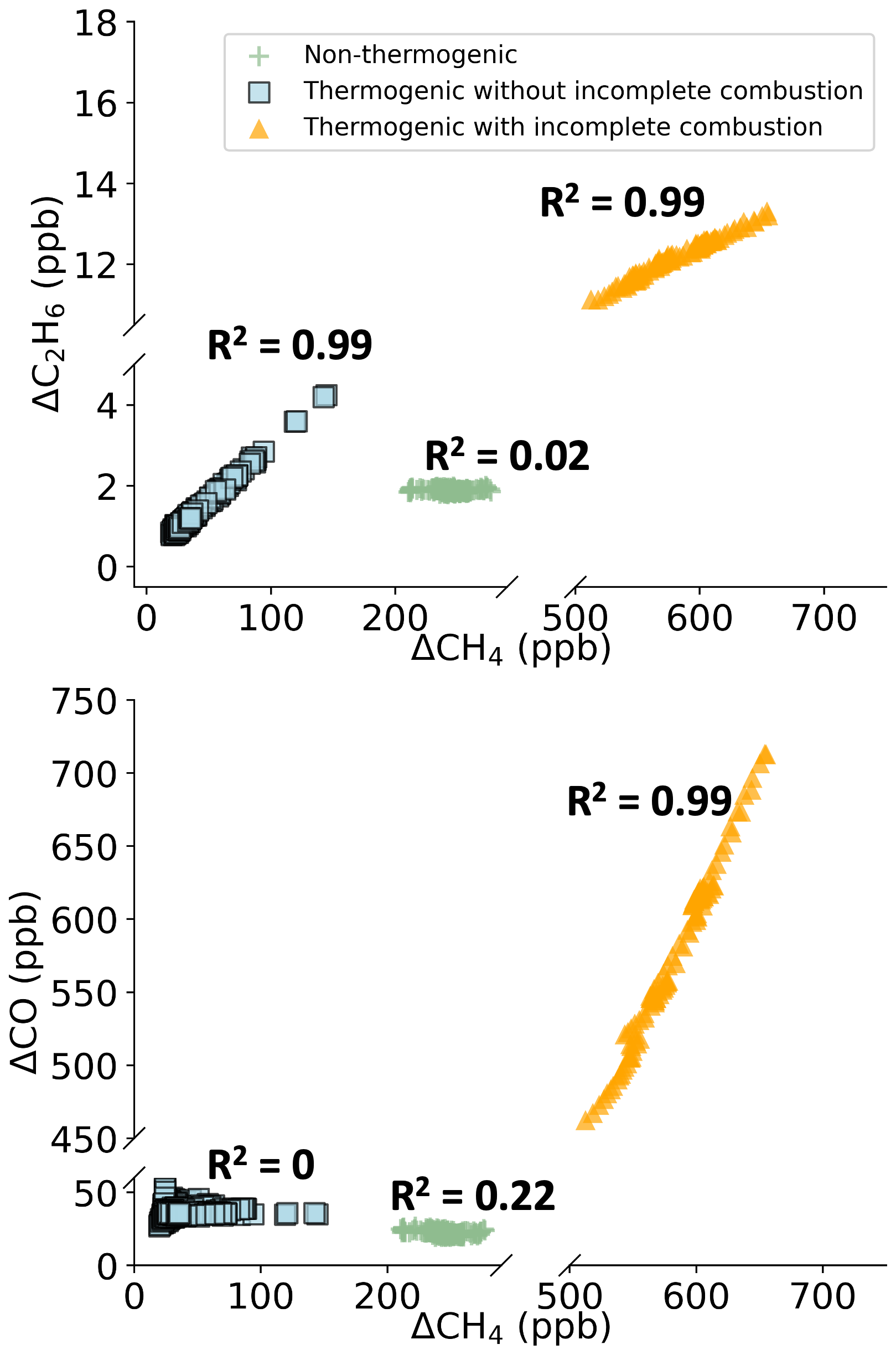
Figure 3 Examples of 1 Hz ΔC₂H₆ : ΔCH₄ and ΔCO : ΔCH₄ from different source types observed over summer 2023 and February 2024. Natural gas-dominated plumes related to pre-meter leaks, such as during the distribution process with $R_{\mathrm{\Delta }{\text{C}}_{\mathrm{2}}{\text{H}}_{\mathrm{6}}:\mathrm{\Delta }{\text{CH}}_{\mathrm{4}}}^{\mathrm{2}}$ ≥ 0.99 & $R_{\mathrm{\Delta }\text{CO}:\mathrm{\Delta }{\text{CH}}_{\mathrm{4}}}^{\mathrm{2}}$ ≤ 0.1 (blue squares, observed on 13 February 2024), natural gas-dominated plumes related to incomplete combustion activities, such as methane from incomplete combustion of natural gas from residential chimneys with $R_{\mathrm{\Delta }{\text{C}}_{\mathrm{2}}{\text{H}}_{\mathrm{6}}:\mathrm{\Delta }{\text{CH}}_{\mathrm{4}}}^{\mathrm{2}}$ ≥ 0.99 & $R_{\mathrm{\Delta }\text{CO}:\mathrm{\Delta }{\text{CH}}_{\mathrm{4}}}^{\mathrm{2}}$ ≥ 0.99 (orange triangles, observed on 11 February 2024), and microbial activity-dominated plumes (often called non-thermogenic sectors) such as landfill, wastewater treatment plants, or natural wetlands with $R_{\mathrm{\Delta }{\text{C}}_{\mathrm{2}}{\text{H}}_{\mathrm{6}}:\mathrm{\Delta }{\text{CH}}_{\mathrm{4}}}^{\mathrm{2}}$ ≤ 0.1 (green crosses, observed on 3 July 2024).

2.6 Simulated methane enhancements

We calculated hourly simulated methane enhancements (ΔCH₄, ppb) by convolving a series of global, national, and regional methane emission inventories (units: nmol m⁻² s⁻¹) with surface influence footprints (ppb (nmol m⁻² s⁻¹)⁻¹) derived from a Lagrangian atmospheric transport model described in Sect. 2.6.3 (Fasoli et al., 2018; Lin et al., 2003):

$$\begin{array}{}\text{(2)}& \begin{array}{rl}\text{Simulated}\mathrm{\Delta }{\text{CH}}_{\mathrm{4}}& =\text{Inventory Emissions}\\ & \times \text{Surface-influence Footprint}\end{array}\end{array}$$

2.6.1 Methane Emission Inventories

We evaluated bottom-up methane emission estimates available at global, national and regional spatial scales (Table S2). (i) At the global scale, we used the anthropogenic monthly 0.1 × 0.1° Emissions Database for Global Atmospheric Research (EDGAR) methane inventories v6.0 and v8.0 for 2018 and 2022 respectively; (ii) at the national scale, we analyzed the anthropogenic monthly 0.1 × 0.1° gridded Environmental Protection Agency (GEPA) inventory and the additional extended version (GEPA Extension) for the year 2018; (iii) at the regional scale, we used the annual 0.02 × 0.02° New York-Newark methane inventory by Pitt et al. (2024), which includes both anthropogenic and natural methane emissions for the New York-Newark area. For consistency, we subset the inventories to the same NYCMA domain and regridded the inventories to a 0.01° × 0.01° spatial resolution to match the surface influence footprint. Many studies have used the U.S. Census Bureau's Topologically Integrated Geographic Encoding and Referencing (TIGER) domain for New York area, which overlaps with most of NYCMA domain used in our study (Pitt et al., 2022, 2024; Nesser et al., 2024; Plant et al., 2019, 2022). Methane emission estimates in NYC from these analyses are thus comparable to results from this study.

• i.

  The EDGAR methane inventories provide global gridded methane emissions using international activity data and the Intergovernmental Panel on Climate Change source sectoral methodology (Crippa et al., 2020; European Commission, Joint Research Centre, 2023; Crippa et al., 2024). Methane emission estimates in EDGAR v6.0 ended in 2018, while EDGAR v8.0 extended activity data through 2022 and updated the residential activity data based on both population density and heating demand (Crippa et al., 2024, 2020). These updates resulted in total methane emissions in EDGAR v8.0 (2022) that were 14.6 % lower than those in EDGAR v6.0 (2018) for NYCMA domain. The GEPA and EDGAR v6.0 methane inventories exhibited similar total methane emissions for 2018 but displayed a low spatial correlation due to EDGAR allocating several large methane point sources to incorrect grid boxes (Fig. S6) (Maasakkers et al., 2023).

• ii.

  GEPA methane inventories allocate sector-specific national anthropogenic methane emissions from the Inventory of U.S. Greenhouse Gas Emissions and Sinks (GHGI) to gridded emissions using proxy datasets (Maasakkers et al., 2023). The extended GEPA methane inventory includes additional emissions from the natural gas end-use sector (post-meter natural gas), primarily allocated based on post-meter activities from the Energy Information Administration (EIA) (Maasakkers et al., 2023). In NYCMA, revised estimates of natural gas emissions in the extended GEPA inventory for 2018 are 65 % (± 14.5 %) larger than those in the main GEPA inventory, with additional post-meter sources accounting for more than 70 % of this increase.

• iii.

  Pitt et al. (2024) developed high-resolution (0.02 × 0.02°) methane inventories for the New York-Newark domain (39.2° N, 42.0° N, 75.7° W, 72.1° W) for 2019, which account for both anthropogenic and natural methane emissions, including post-meter natural gas emissions. Methane emissions from Pitt et al. (2024) are about 1.3 times greater than the 2016 GEPA inventory in the NY-Newark urban area, which is defined using the U.S. Census Bureau's TIGER domain for New York. However, despite these updates, the methane emissions remain a factor of 2.3 lower than estimates based on airborne observations (Pitt et al., 2024, 2022; Maasakkers et al., 2016). Pitt et al. (2024) developed an ensemble of 144 high-resolution methane flux maps by varying spatial distributions and emission factor proxies. We selected 32 out of 144 versions of the Pitt et al. (2024) inventory based on higher mean and median correlation coefficients (R²) between inventory estimates and airborne observations, as reported by Pitt et al. (2024). The Pitt et al. (2024) inventory applied in this study was calculated as the mean of these selected versions.

2.6.2 Non-thermogenic Methane Sources in NYCMA

The dominant non-thermogenic methane sources are microbial in origin and include coastal wetlands, wastewater treatment plants, and landfills. The coastal wetlands in NYCMA are brackish with a seasonal cycle that is expected to peak in summer (Oikawa et al., 2024). Methane emissions from wastewater treatment plants are included in the local methane inventory for NYCMA, but the total number is poorly constrained (Pitt et al., 2024). There are no active landfills in the five boroughs of New York City, and only two active landfills in northern New Jersey within the 75 % surface influence footprints for the Mineola Tower. These landfill methane emissions are included in the inventories, and together are about 1 % of the total methane emissions estimated for February 2024 (EPA, 2024).

2.6.3 Atmospheric Transport Model

The Lagrangian transport model applied in this study simulates hourly footprints, representing the surface influence on the air parcel at the specific moment when the observation is conducted. We used the Stochastic Time-Inverted Lagrangian Transport (STILT) Model to calculate the surface influence footprints. STILT is a Lagrangian particle dispersion model built on the Hybrid Single-Particle Lagrangian Integrated Trajectory (HYSPLIT) system with a distinct turbulent scheme (Fasoli et al., 2018; Lin et al., 2003). STILT calculates sub-grid surface influence footprints from upstream areas in the planetary boundary layer (PBL) by tracing air particles backward in time with the meteorological field at a given location and height. Surface influence footprints quantify how surface emissions contribute to atmospheric trace gas dry mole fractions (Fasoli et al., 2018; Lin et al., 2003). In this study, we coupled STILT with 3 km High-Resolution Rapid Refresh (HRRR) meteorological fields, Benjamin et al., 2016) and configured HRRR-STILT to trace 1000 air particles back 24 h from the Mineola tower site to generate hourly 0.01 × 0.01° surface influence footprints from January 2023 to December 2024. Monthly-mean footprints at Mineola Tower 62 m a.g.l. are shown in Fig. S7.

2.6.4 Uncertainty Assessment

It is difficult to directly quantify the uncertainties in the surface influence footprint calculated by the Lagrangian transport model. Instead, we conducted a sensitivity study using alternative configurations of the atmospheric transport model and convolved the resulting surface influence footprints with the regional methane inventory to simulate a range of methane enhancements (Eq. 2). The observed and simulated monthly mean diel cycles were compared solely to evaluate the sensitivity of the HRRR-STILT transport model to different model configurations and to identify the hours with the most robust model performance for subsequent emissions scaling.

None of the inventories used in this analysis have sub-monthly methane emission variations, so that all of the diel-scale changes in simulated ΔCH₄ are driven by meteorological variation in HRRR-STILT. Schiferl et al. (2025) found that some configurations in HRRR-STILT altered the simulated methane enhancements more than others, especially the value of the minimum mixing layer height (MMLH). HRRR-STILT can calculate the mixed layer height in four ways: (1) sampled directly from the HRRR meteorological model outputs, (2) calculated from the temperature profile, (3) estimated using the turbulence kinetic energy, and (4) computed from the modified Richardson number (default). We evaluated the variability of the surface influence footprint calculated using these different configurations for May to August 2023. We also conducted sensitivity tests using different minimum mixed layer heights of 150 and 250 m. We found that the choice of method to calculate mixed-layer height and the value of minimum mixed-layer height makes less than 1 ppb difference in the simulated methane enhancements during the afternoon when the boundary layer is high and well-mixed (Figs. S8 and S9). We also found that the simulated diel variability of ΔCH₄ closely matches the observed diel pattern, suggesting that the Lagrangian transport model HRRR-STILT captured the overall atmospheric dynamics for the NYCMA (Fig. S10). We adopted the default Richardson Number method to calculate the mixed-layer height with the default 150 m minimum height. We used only afternoon observations (12:00 to 18:00 local time), when HRRR–STILT simulations are least sensitive to model configuration choices, to quantify monthly methane emissions from the NYCMA.

We compared the monthly mean diel cycle of the observed and simulated ΔCH₄. The best agreement between observed and simulated ΔCH₄ was observed in May, especially in the afternoon (gray shading). Among the inventories, Pitt et al. (2024) consistently demonstrated the closest match to the observations and smallest underestimation of ΔCH₄, while EDGAR had the largest underestimate in almost every month. This discrepancy with EDGAR may reflect known issues with spatial allocation errors for large point sources in the Northeast U.S. region (Fig. S6).

2.7 Observation-informed Methane Emissions

We calculated observation-informed methane emissions by applying a simulated scaling factor (SF) to the corresponding regional, national and global inventories over the NYCMA. The SF allows us to capture biases in inventory methane emissions while minimizing the impact of meteorological variability, and is widely applied in other studies over urban areas (Schiferl et al., 2025, 2024; Sargent et al., 2021). The simulated SF normalizes the observed methane enhancements by the simulated enhancements (Eq. 3):

$$\begin{array}{}\text{(3)}& \text{Simulated SF}={\displaystyle \frac{\mathrm{\Delta }{\text{Observed CH}}_{\mathrm{4}}}{\mathrm{\Delta }{\text{Simulated CH}}_{\mathrm{4}}}}\end{array}$$

A simulated SF greater than one indicates that methane emissions are underestimated by the inventory, while a value less than one suggests that the inventory overestimates methane emissions. In this study, we calculated the afternoon SF for each month by applying 10 000 bootstrapping draws with replacement for paired $\frac{\mathrm{\Delta }{\text{Observed CH}}_{\mathrm{4}}}{\mathrm{\Delta }{\text{Simulated CH}}_{\mathrm{4}}}$ with background variation. The SF calculations require at least 80 afternoon hours of valid paired observed and simulated ΔCH₄ for each month.

We then calculated the observation-informed methane emissions for each month (Eq. 4) using

$$\begin{array}{}\text{(4)}& \begin{array}{rl}& \text{Observation-informed Emissions}=\\ & \text{Inventory Emissions}\times \text{Simulated SF}\end{array}\end{array}$$

We quantified monthly observation-informed methane emissions for the afternoon only (12:00 to 18:00 EDT) and calculated the mean and 95 % CI for each month by bootstrapping from the hourly observation-informed methane emissions derived from all inventories during the afternoon (12–18 h), The 95 % CI accounts for uncertainties in the ensemble of various methane inventories, background calculations, and variations in hourly observed and simulated ΔCH₄.

2.8 Methane Loss from Natural Gas Sectors

Previous studies have typically compared natural gas consumption with methane emissions using linear regression to quantify the natural gas methane loss rate in urban areas. This has been done either by (a) comparing natural gas methane consumptions with total estimated methane emissions (Karion et al., 2023b; Zeng et al., 2023; He et al., 2019), or (b) comparing natural gas methane consumptions with only the thermogenic portion of total methane emissions (Sargent et al., 2021; McKain et al., 2015). In this study, we explored both methods by calculating two cases of methane loss rates using different sets of estimated methane emissions: (1) observation-informed total methane emissions and (2) observed ΔC₂H₆ : ΔCH₄ ratio inferred thermogenic methane emissions.

We used county-resolved natural gas deliveries to NYC (New York, Kings, Queens, Bronx, and Richmond counties) (S&P Global, 2025b) and northeast New Jersey (NE NJ; Bergen, Hudson, Passaic, Essex, Union, Middlesex, and Monmouth counties) (S&P Global, 2025a). The total methane delivered from the natural gas sector was calculated by multiplying monthly natural gas deliveries by the corresponding mean monthly natural gas methane percentage reported across three pipeline companies operating in NYCMA: Transco, Tetco, and Iroquois (assuming standard conditions of 60 °F and 14.7 psia) (Williams Companies, 2025; Enbridge, 2025; Iroquois Gas Transmission System, LP, 2025).

We calculated the slope of the RMA linear regression to compare monthly observation-informed methane emissions with monthly natural gas methane delivered to NYC and NE NJ using two methods:

1. We applied Model II RMA regression in R (gives the mean linear fit and 95 % CI) to total monthly observation-based methane emissions and the total natural gas methane delivered to the NYCMA and northeast NJ for all months in 2023 and 2024. Here, we added NYCMA city core observation-based wintertime methane emissions from Schiferl et al. (2025) for additional long-term constraints, but the inclusion of this data does not change any results.

2. Adapting the methodologies of Sargent et al. (2021), and McKain et al. (2015), we estimated observation-based natural gas methane emissions by scaling total methane emissions by the thermogenic fraction calculated as the ratio of monthly observed ΔC₂H₆ : ΔCH₄ ratios to the monthly ΔC₂H₆ : ΔCH₄ ratios of thermogenic plumes ($R_{\mathrm{\Delta }{\text{C}}_{\mathrm{2}}{\text{H}}_{\mathrm{6}}:\mathrm{\Delta }{\text{CH}}_{\mathrm{4}}}^{\mathrm{2}}\ge \mathrm{0.95}$). We applied a Model II RMA linear regression to the observation-based natural gas methane emissions and the total natural gas methane delivered to NYC and northeast NJ.

3 Results

We observed a strong seasonal cycle in observation-informed monthly methane emissions from January 2023 to December 2024, with peaks in months with winter heating and summer cooling loads. We found that thermogenic methane is the dominant source in both seasons, and the incomplete combustion of natural gas was the major signal observed. From the thermogenic methane emissions and delivered natural gas methane rates, we calculated a methane loss rate that is not included in the national methane inventory.

3.1 Observation-informed Methane Emission Rates

We identified seasonal variations in methane emissions from NYCMA from January 2023 to December 2024 (Fig. 4), with larger uncertainties during summertime possibly driven by background variation and wetland activities. The observation-informed emissions were high in winter months with building heating loads (in January and February), decreased from March to a minimum in May (two-year average of 6.3 ± 4.3 kg s⁻¹), and increased again in months with building cooling loads (June, July and August). Methane emissions increased further in the following heating season, with yearly maxima in November 2023 (15.9 ± 4.4 kg s⁻¹) and October 2024 (17.5 ± 4.8 kg s⁻¹), Monthly observation-informed methane emissions with 95 % CI can be found in Table S3.

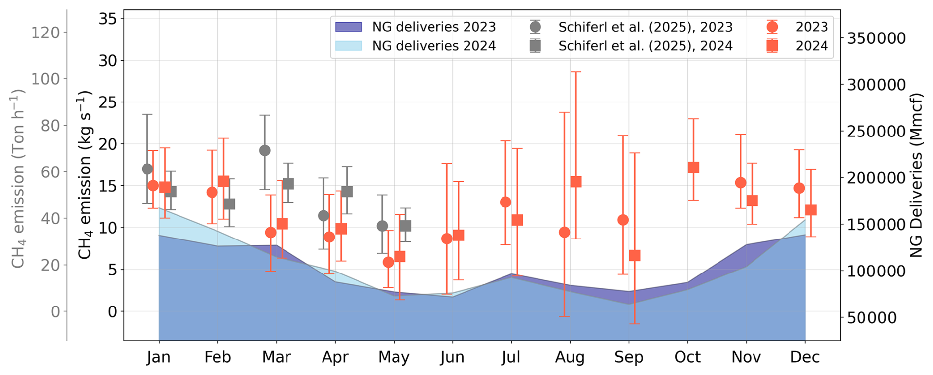
Figure 4 Observation-informed mean monthly methane emission rates from January to December in 2023 (red circles with 95 % CI error bars) and 2024 (red squares, 95 % CI error bars) for the NYCMA. Monthly observation-informed wintertime methane emissions from Schiferl et al. (2025) for NYCMA urban core are shown in grey (2023 in circles, and 2024 in squares). Total natural gas deliveries to the NYCMA (in units of MMcf, Million cubic feet) are indicated in dark blue shading for 2023, and light blue shading for 2024.

The seasonal cycle of NYCMA methane emissions quantified using suburban Mineola Tower measurements is consistent with the methane emissions Schiferl et al. (2025) using city core observations, which saw peak methane emissions in January and February, followed by a decline into spring. The 75 % percentile footprint at Mineola Tower encompasses the majority of the urban areas within the NYCMA (Fig. 1), including northeastern New Jersey, Manhattan, the Bronx, and western Long Island. This footprint largely overlaps with the 75 % percentile footprint reported by Schiferl et al. (2025) for their urban core site, providing a robust spatial basis for comparison between the two studies. In general, the suburban observation-informed methane emissions in the spring months are slightly lower than the city core estimates, except in February 2023. The largest disagreement occurred in March of 2023, likely driven by reduced sampling at the urban core site, where they captured a high-emission period at the end of the month (Fig. S11).

We observed a more pronounced seasonal cycle at the Mineola Tower compared with previous airborne-based methane emission estimates from before 2020. During the wintertime, we observed higher methane emissions (two-year averages of 13.2 ± 8 kg s⁻¹ in November, February, and March) than airborne-based estimates in the same month from 2018–2020 (9.7 ± 4.4 kg s⁻¹, Pitt et al., 2022). But we observed lower methane emissions during the warmer months of April (2023: 9.0 ± 4.7 and 2024: 9.9 ± 4.1 kg s⁻¹) and May (2023: 6.0 ± 3.4 and 2024: 6.5± 5.1 kg s⁻¹) than estimated from aircraft in April 2018 (14.3 ± 8.6 kg s⁻¹, Plant et al., 2019).

3.2 Methane Emissions from Thermogenic Sources

We observed that thermogenic sources dominated NYCMA methane emissions in the summer cooling and winter heating season. Thermogenic sources accounted for nearly all methane emissions in months with building heating loads (February and May; 98 % thermogenic), whereas in months with building cooling loads (June, July, and August) there was a 12 % to 15 % non-thermogenic contribution. Tower observation-based thermogenic fractions are higher than previous studies using short-term airborne measurements. Among thermogenic plumes, incomplete combustion of natural gas was the major signal observed. Thermogenic sources were dominant during both the summer cooling and winter heating season, and previous widely-applied approaches relying solely on fixed pipeline compositions tend to underestimate the thermogenic methane contribution in urban regions. As shown in Fig. 5a, the estimated thermogenic methane fraction using this method was 88 ± 7 % in June, 85 ± 11 % in July, and 85 ± 12% in August. In the NYCMA heating season, we estimated thermogenic methane fractions of 99 ± 4 % in February and 98 ± 9 % in May. Floerchinger et al. (2021) calculated a thermogenic fraction of 81.5 % (+0.4 %, −0.6 %) for New York City during the summer months using airborne observations and the local pipeline ethane-to-methane ratio (Floerchinger et al., 2021). Plant et al. (2019) estimated a thermogenic methane contribution of 87 ± 10 % in winter using the airborne ethane-to-methane ratio compared with the Transco pipeline (Plant et al., 2019). These source attribution estimates fall within, but at the lower end of, our seasonal range.

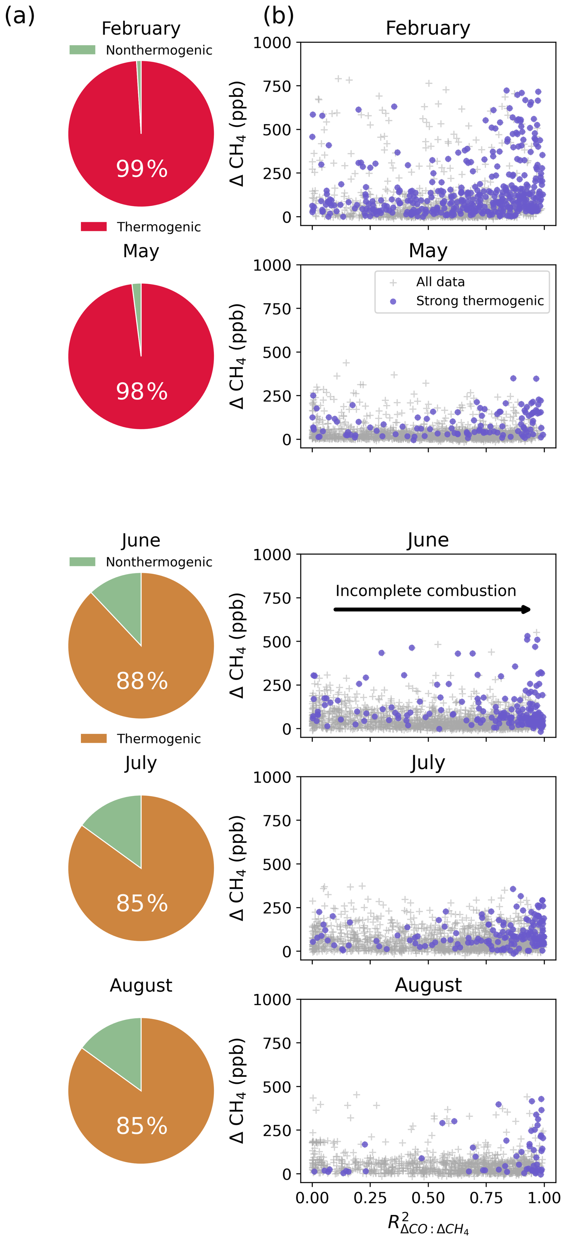
Figure 5 Monthly thermogenic fraction of total methane emissions and monthly incomplete combustion of natural gas signals. (a) Monthly thermogenic (red for heating season and orange for cooling months) and non-thermogenic (green) fractions of methane emissions. (b) Plot of 5 min average ΔCH₄ as a function of the correlations between 1 Hz ΔCO and ΔCH₄ within each 5 min interval for thermogenic plumes ($R_{\mathrm{\Delta }{\text{C}}_{\mathrm{2}}{\text{H}}_{\mathrm{6}}:\mathrm{\Delta }{\text{CH}}_{\mathrm{4}}}^{\mathrm{2}}\ge \mathrm{0.95}$, purple circle) and all 5 min interval observations (gray cross).

Incomplete combustion of thermogenic sources is the dominant signal observed at Mineola Tower. We analyzed high-frequency (1 Hz) RMA correlations between ΔCO and ΔCH₄ within each 5 min interval with $R_{\mathrm{\Delta }{\text{C}}_{\mathrm{2}}{\text{H}}_{\mathrm{6}}:\mathrm{\Delta }{\text{CH}}_{\mathrm{4}}}^{\mathrm{2}}\ge \mathrm{0.95}$, which represent thermogenic plumes with limited atmospheric mixing. A larger fraction of these thermogenic plumes exhibit high $R_{\mathrm{\Delta }\text{CO}:\mathrm{\Delta }{\text{CH}}_{\mathrm{4}}}^{\mathrm{2}}$ (Fig. 5b). The majority of $R_{\mathrm{\Delta }\text{CO}:\mathrm{\Delta }{\text{CH}}_{\mathrm{4}}}^{\mathrm{2}}$ values exceed 0.7 during months with building heating demand (median of thermogenic $R_{\mathrm{\Delta }\text{CO}:\mathrm{\Delta }{\text{CH}}_{\mathrm{4}}}^{\mathrm{2}}>\mathrm{0.7}$ during heating season), and exceed 0.8 during months with building cooling demand (median of thermogenic $R_{\mathrm{\Delta }\text{CO}:\mathrm{\Delta }{\text{CH}}_{\mathrm{4}}}^{\mathrm{2}}>\mathrm{0.8}$ during cooling season) (Fig. S12). Thermogenic plumes with moderate $R_{\mathrm{\Delta }\text{CO}:\mathrm{\Delta }{\text{CH}}_{\mathrm{4}}}^{\mathrm{2}}$ (between 0.1 and 0.8) are observed more frequently during months with building heating loads (Fig. S12), suggesting greater variability in combustion efficiency, likely driven by various natural gas combustion processes for heating purposes. These consistently high 1 Hz ΔCO : ΔCH₄ correlations across seasons demonstrate that incomplete combustion of natural gas is the dominant thermogenic methane process during both building heating and building cooling seasons. In contrast, only 7 % (summer) and 6 % (winter) of the identified thermogenic plumes were observed to have no combustion signature ($R_{\mathrm{\Delta }\text{CO}:\mathrm{\Delta }{\text{CH}}_{\mathrm{4}}}^{\mathrm{2}}<\mathrm{0.1}$), showing that natural gas emissions from pipeline leaks were less frequently observed at the Mineola tower compared to combustion-related natural gas sources. Similarly, Schiferl et al. (2025) identified incomplete combustion activities as a major contributor to wintertime methane emissions over NYCMA (Schiferl et al., 2025) using six years of observations. And the thermogenic methane emissions driven by incomplete combustion of natural gas is a plausible explanation for why cities such as Boston have shown little to no decrease in methane emissions despite extensive efforts to repair natural gas pipeline leaks (Sargent et al., 2021).

3.3 Methane Loss Rate

There were strong positive linear relationships between observation-based thermogenic methane emissions and natural gas methane deliveries (R²=0.90) (Fig. 6). This pattern is consistent with thermogenic methane emissions that are primarily driven by post-meter end-use in the natural gas sector. These thermogenic emissions are proportional to natural gas consumption, while emissions from the local distribution system, which operates under relatively constant pipeline pressure, may remain stable throughout the year. The consumption-driven natural gas methane loss rate inferred from observed thermogenic ΔC₂H₆ : ΔCH₄ ratios is 1.7 ± 0.6 % (95 % CI), which is more than three times higher than the natural gas loss rate of 0.5 % applied in the most recent bottom-up methane inventory for the NYCMA (Pitt et al., 2024). Comparing total methane emissions with delivered natural gas methane yielded a weaker correlation (R²=0.28) and an estimated loss rate of 1.3 ± 0.7 % (Fig. S13). The lower agreement likely reflects additional contributions from microbial sources such as wetlands during warmer months, a pattern also observed in Boston (Sargent et al., 2021). However, even when using total methane emissions, the inferred methane loss rate remains nearly 2.5 times higher than bottom-up estimates in the NYCMA (Pitt et al., 2024).

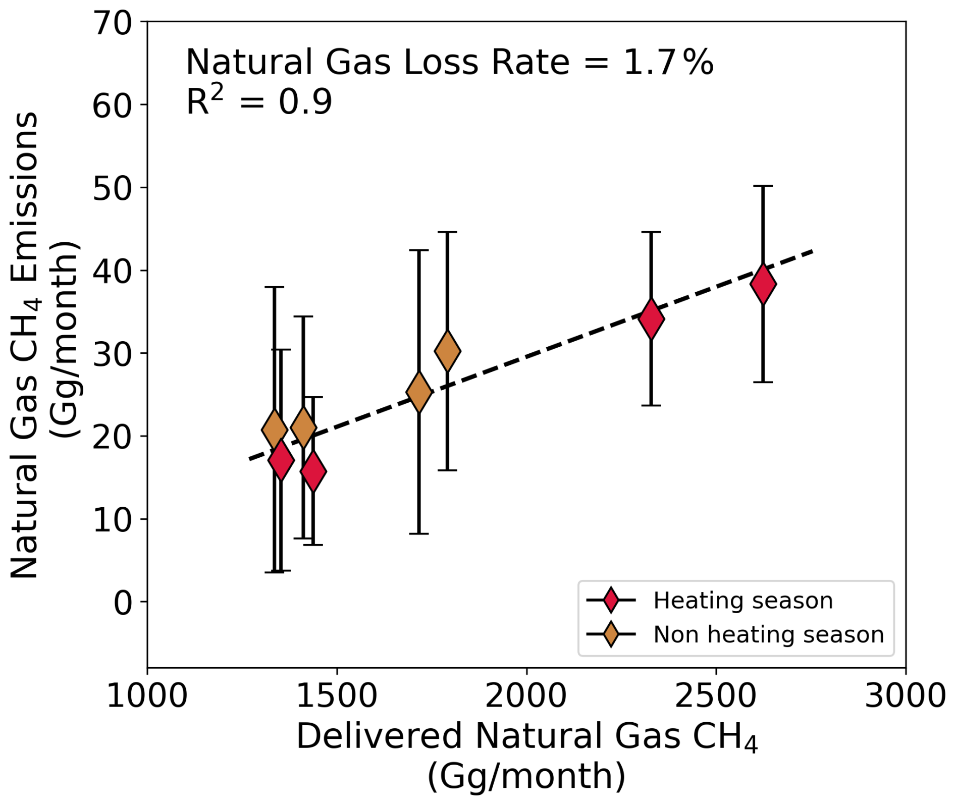
Figure 6 Observation-based natural gas methane emissions compared to natural gas methane delivered to NYC and northeast NJ for natural gas methane emissions using the observed ΔC₂H₆ : ΔCH₄ ratio for heating (red diamonds; February, May) and non-heating (orange diamonds; June, July).

4 Conclusion and Discussion

We identified a distinct seasonal cycle in methane emissions across the NYCMA for 2023 and 2024. Observation-informed methane emissions peaked during the months with building heating (winter) and cooling (summer) loads, and declined steadily in the shoulder seasons. This temporal pattern correlates with peaks in natural gas deliveries for both winter heating and summer cooling seasons. With global temperatures continuing to rise, leading to more frequent, prolonged, and intense extreme weather events, including extreme heat and extended cold periods, energy demand for both cooling and heating is expected to grow. Without a transition to cleaner energy sources, this increased energy demand could lead to higher methane emissions in urban regions.

Source attribution analysis reveals that the incomplete combustion of natural gas (post-meter emissions from the inefficient burning of natural gas in any appliance or power unit) dominates methane emissions in the city, regardless of season. There is no natural gas methane loss rate currently included in national or global inventories (Crippa et al., 2024; Maasakkers et al., 2023), but the local NYCMA inventory (Pitt et al., 2024) has included a beyond-the-meter loss rate of 0.5 % (Fischer et al., 2018). However, we calculated a consumption-driven loss rate for the NYCMA that is a factor of three times greater than these previous studies of appliance emissions. These largely overlooked combustion-related post-meter methane emissions can help explain the persistent missing thermogenic methane sources reported by previous studies.

The observed loss rate of 1.7 ± 0.6 % is within the range observed for other cities. It is less than the 2.5 ± 0.5 % (Sargent et al., 2021) and 2.7 ± 0.6 % (McKain et al., 2015) reported for the Boston area, but greater than the lower limit of the 1.3 %–2.3 % reported for Los Angeles (He et al., 2019; Sargent et al., 2021) and the 1.3 % reported for the Baltimore/DC area (Huang et al., 2019).

Many cities, including Boston, have dedicated millions of dollars to upgrading street-level natural gas infrastructure, without seeing any substantial change in methane emissions (Sargent et al., 2021). At the monthly retail prices of natural gas for 2023 and 2024, a 1.7 % loss rate is close to 300×10⁶ USD yr⁻¹ of natural gas purchased, but unused, by consumers in NYCMA.

Our results highlight the three dimensional nature of urban methane emissions: the largest methane emissions are observed from rooftops and not from the pipelines beneath the streets below. Our findings emphasize the urgent need to incorporate emissions from post-meter natural gas combustion into methane inventories and emphasize emissions reductions from natural gas end-use sectors as a means to reduce urban methane emissions.