Coastal upwelling and tropical warm water intrusions are key drivers of interannual fog variability along the southwestern African coast

Fog and low clouds (FLCs) are a key source of moisture for ecosystems in the Namib Desert, yet their variability and underlying mechanisms remain poorly quantified. We investigate monthly FLC cover in two fog hotspots: the Angolan Namib (15–17° S) and the Central Namib (22–24° S), using satellite-based observations from 2004 to 2019. Assuming that most fog originates from advected marine low clouds, we apply a cloud-controlling factor framework in which FLC anomalies are modeled as a linear function of spatial anomaly fields in estimated inversion strength (EIS), relative humidity at 700 hPa (R700), sea surface temperature (SST), and the eastward and northward components of the 10 m wind (U10 and V10). Sensitivities of FLCs to these drivers are quantified using a statistical model. Results indicate positive sensitivities to coastal EIS, negative sensitivities to R700, localized negative sensitivities to SST, and a strong influence of onshore circulation, consistent with an advective origin of fog in the Namib region. The statistical models are then used to reconstruct historical FLC anomalies for 1982–2019 using reanalysis data. The reconstructions reveal near-zero trends resulting from opposing influences: increased atmospheric stability enhances FLCs, while SST warming counteracts this. Finally, the reconstructions are used to assess interannual variability and its links to climate modes. Benguela Niño events, associated with tropical water intrusion and SST warming, explain up to half of the interannual FLC variability in the Angolan Namib, with warmer SSTs reducing FLC cover. El Niño conditions also enhance FLC occurrence, but their influence is much weaker.

1 Introduction

The Namib Desert, located along the southwestern coast of Africa, is considered the oldest desert on Earth, already semi-arid around 55 million years ago and reaching extreme aridity between 10–7 million years ago (Huntley, 2023). Today, it remains one of the driest places on Earth. Despite these hyper-arid conditions, it is home to a large number of plant and animal species, several of which are endemic (Griffin, 1998; Juergens et al., 2013). The survival of most of these species relies on the moisture supplied by fog (Louw and Holm, 1972; Seely and Henschel, 1998; Ebner et al., 2011; Warren-Rhodes et al., 2013; Wang et al., 2019). Additionally, fog can transport nutrients and pollutants (Weathers et al., 2020), which can influence local biogeochemistry (Warren-Rhodes et al., 2013; Gottlieb et al., 2019). With climate projections indicating warmer and drier conditions for Southern Africa (Maúre et al., 2018), fog may play an increasingly important role in maintaining regional ecosystems under climate change.

In the region, several fog types can be identified. First, there is advection fog, which forms when moist air masses are transported over a cool ocean surface (Gultepe et al., 2007). Advection fog is typically confined to a narrow coastal strip (Seely and Henschel, 1998), and can depend on the spatial extent of cold-water upwelling (Olivier and Stockton, 1989). Further inland, advected marine stratus clouds, which become fog when the cloud base intersects the surface (also called “high fog” in Seely and Henschel, 1998), dominate. High fog is most frequent between September–March and extends up to 100 km inland (Lancaster et al., 1984; Seely and Henschel, 1998; Andersen et al., 2019; Malik et al., 2026; Hipler et al., 2026). Both high fog and advection fog are generally regarded as being of marine and advective origin, but they differ in where saturation occurs and in the atmospheric processes leading to surface fog. Analyses of stable isotopes in fog water samples (Kaseke et al., 2017, 2018) have been interpreted as an indication for the presence of radiation fog, i.e. fog forming locally at the land surface due to radiative cooling under clear-sky conditions (Gultepe et al., 2007). However, such radiation fog events are likely rare when considering the Namib as a whole. Given the extensive research supporting the dominance of advective processes (Olivier and Stockton, 1989; Seely and Henschel, 1998; Andersen et al., 2019; Spirig et al., 2019; Andersen et al., 2020), this study assumes that the majority of fog has an advective origin. As our satellite-based product cannot reliably distinguish between coastal advection fog and inland high fog, and both are linked to marine advective processes, these are hereafter grouped and referred to as fog and low clouds (FLCs).

Two regional fog hotspots in the Namib Desert are the Central Namib (CN; 22–24° S) and the Angolan Namib (AN; 15–17° S), as shown in Fig. 1 (Andersen and Cermak, 2018; Andersen et al., 2019). Both regions feature a narrow coastal plain that transitions to a central plateau in the CN and steeper mountains in the AN. However, these regions are associated with different cells of the Benguela upwelling system (Nelson and Hutchings, 1983), and feature different peak seasons of fog occurrence (Andersen et al., 2019). Upwelling is a key component of fog formation in the Namib Desert, as marine air advected over cold upwelled water cools towards saturation (Olivier and Stockton, 1989). The AN region is located near the Cape Frio (18° S) upwelling cell, which exhibits a pronounced seasonal cycle, with strong upwelling of cold subsurface waters during winter and spring. This seasonality is primarily driven by relaxation of the trade winds, resulting in the intrusion of warm tropical waters during summer and a decrease in upwelling intensity. In contrast, the CN region lies downwind of the Lüderitz (26° S) upwelling cell, where upwelling is generally weaker than at Cape Frio during winter and spring but persists throughout the year (Andrews and Hutchings, 1980; Hutchings et al., 2009). However, day-to-day fog variability in the CN has only been found to be weakly associated with upwelling at Lüderitz in austral autumn, likely because SST pattern effects are more pronounced at longer time scales (Andersen et al., 2020). Additionally, teleconnections to El Niño-Southern Oscillation (ENSO) have been suggested to enhance fog occurrence in the Central Namib during El Niño conditions, through increased moisture advection associated with more frequent northwesterly winds (Li et al., 2025). However, this relationship is based on observations from a single location and is mainly evident during the most recent decade of the record, motivating further investigation of ENSO-related FLC variability across the Namib Desert.

Here, a cloud-controlling factor (CCF) framework (Klein et al., 2017) is applied to predict large-scale FLC anomalies in the AN and the CN using anomalies of large-scale meteorology. We extend the traditional CCF framework to account for advection patterns and non-local effects, i.e. the influence of conditions occurring outside the AN and CN regions themselves, such as SST anomalies associated with upwelling cells located upwind of them, by using spatial predictor fields (Andersen et al., 2020; Ceppi and Nowack, 2021; Ceppi et al., 2026). The first goal of this study is to quantify the sensitivities of FLCs to selected CCFs and assess whether these sensitivities point towards the advective nature of fog in the region. The hypothesis is that the CCF sensitivities reveal known sensitivities of marine low clouds: a negative relationship to SSTs, a positive relationship to coastal EIS, and an important role for onshore circulation. The second goal is to assess how regional and large-scale SST variability influences interannual fluctuations of FLCs. The hypothesis is that regional SST variability is a primary control of interannual FLC variability.

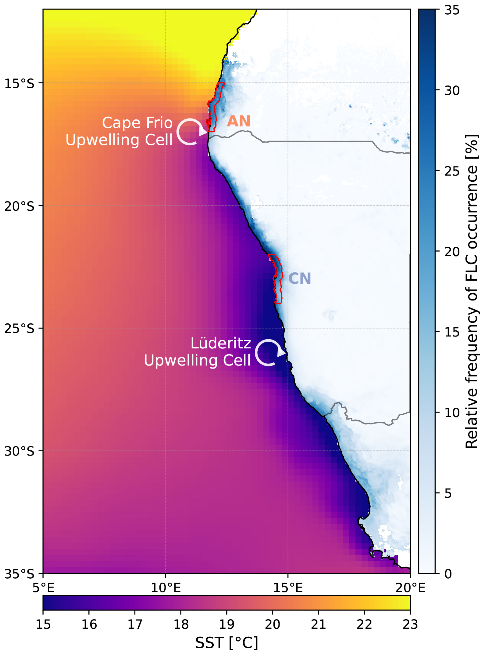
Figure 1 Spatial distribution of sea surface temperatures and relative frequency of fog and low cloud (FLC) occurrence along the southwestern African coast. SST [°C] is shown over the ocean in purple to yellow shades and FLC occurrence frequency [%] over land in blue shades, giving an overview of both the upwelling regions and the areas of frequent fog occurrence. The two regions are outlined in red: Angolan Namib (AN) and Central Namib (CN). The Cape Frio upwelling cell and the Lüderitz upwelling cell are marked with white circular arrows.

2 Data and methods

2.1 Satellite-based FLC cover

A FLC cover metric is derived from the FLC detection algorithm created by Andersen and Cermak (2018). This algorithm relies on data from the Spinning Enhanced Visible and Infrared Imager (SEVIRI) onboard the Meteosat Second Generation (MSG) satellites. SEVIRI provides spatiotemporally continuous observations with a spatial resolution of 3 km at nadir and a temporal resolution of 15 min (Schmetz et al., 2002). The FLC detection algorithm identifies FLCs consistently during all times of day by combining infrared measurements with a set of threshold-based and image-analysis techniques. Validation against nighttime surface net radiation measurements from the FogNet station network (Kaspar et al., 2015) in the central Namib, which accurately capture the presence of low cloud, demonstrates good performance, with a probability of detection of 94 %, a false-alarm rate of 12 %, and an overall classification accuracy of 97 % (Andersen and Cermak, 2018). It should be noted, however, that this satellite-based method cannot on its own distinguish between fog and low stratus clouds, as it is not straightforward from a satellite perspective to determine whether the cloud base is in contact with the surface. Cloud base height can be estimated by combining the satellite product with additional near-surface relative humidity data (Malik et al., 2026), but such an estimate is not required for our analysis, and fog and low clouds are therefore grouped together throughout.

The algorithm outputs a binary field of FLC occurrence at 15-min temporal resolution for each spatial grid cell. From these binary data, a daily, cell-based FLC cover metric is calculated as the relative occurrence frequency [%] for each cell, based on a 24 h period starting at 12:00 UTC. This definition accounts for the diurnal cycle of FLC occurrence, which typically has a minimum at 12:00 UTC (14:00 Central Africa Time, CAT), increases during the night, and peaks at 04:00–06:00 UTC (06:00–08:00 CAT) (Andersen and Cermak, 2018). The advective nature of FLCs leads to high occurrence at the coast that progressively decreases farther inland (see Fig. 1); to enhance the signal-to-noise ratio, the analysis is restricted to grid cells within 24 km of the coastline along the coastal plain, within the latitudinal bounds of each region (AN: 15–17° S; CN: 22–24° S). The daily, cell-based FLC cover is first spatially averaged over all valid grid cells within this domain, yielding a single daily regional value, which is then temporally averaged over each calendar month to derive the monthly FLC cover time series for the AN and CN regions over the 2004–2019 period. This monthly, domain-averaged FLC cover time series serves as the predictand in the statistical model (see Sect. 2.3).

2.2 Cloud-controlling factors

In this study, five cloud-controlling factors were selected as predictors for the statistical model (see Sect. 2.3). These factors follow the convention of standard cloud-controlling-factor frameworks for low clouds (Klein et al., 2017; Scott et al., 2020; Ceppi and Nowack, 2021; Andersen et al., 2022). The predictors used are the estimated inversion strength (EIS), relative humidity at 700 hPa (R700), sea surface temperature (SST), and the eastward and northward components of the wind at 10 m above the surface (U10 and V10, respectively). These variables represent key processes known to influence marine low clouds. EIS characterizes the strength of the capping inversion and therefore influences the mixing of free-tropospheric and boundary-layer air. R700 represents the humidity of the free troposphere above the cloud layer and can influence both cloud-top radiative cooling and entrainment processes. SST affects boundary-layer stability and the thermodynamic contrast between the ocean surface and the overlying air mass. Finally, U10 and V10 capture near-surface circulation, both the advection of FLCs toward the coast and inland, and boundary layer dynamics (Klein et al., 2017). Standard CCF frameworks typically use wind speed instead, which captures surface fluxes and mixing but carries no directional information. Because the direction of the flow is crucial for FLCs in the Namib Desert, the wind is decomposed into its eastward and northward components rather than represented by speed alone, which better captures the onshore advection of FLCs. Subsidence was tested as an additional predictor but was excluded from the final set, as it did not provide additional predictive information within our modelling framework. This does not imply that subsidence is physically unimportant for FLCs, but rather that it did not provide additional usable information for predicting FLC cover anomalies at the spatial and temporal scales considered here. Horizontal temperature advection is indirectly represented through the spatial SST fields and U10 and V10. Finally, based on Mass et al. (2025), it was found that biomass burning aerosols (BBA) may contribute to FLC persistence via semi-direct effects, but were found to be hard to separate from meteorological effects. As the analysis of Mass et al. (2025) suggests that semi-direct effects may be captured in the EIS fields already, we do not include BBA, or other aerosols, as CCFs here.

Similarly to Scott et al. (2020), monthly sea surface temperature (SST) fields from the National Oceanic and Atmospheric Administration (NOAA) Optimum Interpolation (OI) SST product, version 2 (Huang et al., 2021), were used. This dataset provides spatially complete SST fields constructed by merging satellite, ship, and buoy observations. All other meteorological fields were obtained from the ERA5 (Hersbach et al., 2020) reanalysis in one configuration and from the MERRA-2 (Gelaro et al., 2017) reanalysis in another. The EIS is computed based on the method developed by Wood and Bretherton (2006). NOAA OI SST and ERA5 have a horizontal resolution of 0.25° latitude × 0.25° longitude, whereas MERRA-2 has a resolution of 0.5° latitude × 0.625° longitude. To ensure consistency across datasets, all variables were regridded to the MERRA-2 grid via bilinear interpolation. Monthly averages for the period 1982–2019 were used for all datasets. Because the NOAA OI SST dataset begins in September 1981, starting in 1982 ensures a complete first year of data.

To reduce the dimensionality of the predictor set and to avoid relying on inland wind fields, where the two reanalyses differ (see Figs. B4 and B5), the R700, U10, and V10 fields were masked over land, so that only oceanic grid points were retained as predictors for these three variables. This also ensures consistency across all predictors, as they now share the same spatial extent.

To analyze the influence of SST on the interannual variability of FLC cover, several ocean indices were calculated. The Benguela Niño Index (BNI) was defined, following McPhaden et al. (2024), using the NOAA OI SST dataset as the area-averaged SST anomaly over 10–20° S, 8–14° E. SST anomalies were calculated relative to the 1991–2020 climatology, and a long-term linear trend of 0.33 °C per decade was removed from the resulting BNI time series. Similarly, the Lüderitz Upwelling Cell Index (LUCI) was defined as the area-averaged, detrended, and deseasonalized SST anomalies over 24–28° S, 12–15° E. Finally, consistent with Espinoza et al. (2024), the Oceanic Niño Index (ONI) was obtained from the National Centers for Environmental Prediction (NCEP) for the period 1982–2019. The ONI represents 3-month running mean sea surface temperature (SST) anomalies in the Niño 3.4 region (5° N–5° S, 120–170° W) (Glantz and Ramirez, 2020). The relationship between the SST-based indices and the reconstructed FLC anomalies at different time lags is quantified using lagged Pearson correlations. Prior to this analysis, all series are smoothed with a 3-month centred running mean, consistent with the definition of the ONI. For a lag of k months, the FLC anomaly series is correlated with the index series shifted k months earlier, such that positive lags correspond to the index leading the FLC cover anomalies.

2.3 Statistical learning framework

In this study, a statistical learning analysis is developed to quantify the sensitivities of the key drivers (see Sect. 2.2) controlling FLC cover in the Namib Desert. The method builds on the cloud-controlling factors framework (Klein et al., 2017; Scott et al., 2020; Ceppi and Nowack, 2021; Andersen et al., 2023), in which the FLC cover anomalies over the AN or CN region r, denoted dF(r), are modeled as a linear function of the anomalies of P relevant meteorological cloud-controlling factors dX_i(r):

$$\begin{array}{}\text{(1)}& {\displaystyle }{\displaystyle }\mathrm{d}F\left(r\right)\approx \sum _{i=\mathrm{1}}^P{\displaystyle \frac{\partial F\left(r\right)}{\partial X_i\left(r\right)}}\cdot \mathrm{d}{X}_i\left(r\right)=\sum _{i=\mathrm{1}}^P{\mathit{\omega }}_i\left(r\right)\cdot \mathrm{d}{X}_i\left(r\right),\end{array}$$

where ω_i(r) represents the sensitivity of dF(r) to the ith controlling factor anomaly.

Similar to Ceppi and Nowack (2021), this study moves beyond local grid-point-wise relationships between dF(r) and dX_i(r) by averaging the FLC cover anomaly over the AN and CN regions and expressing it as a function of the controlling factor anomalies within a 25° latitude × 15° longitude area (10–35° S, 5–20° E). This area was chosen to encompass the majority of the synoptic-scale variability of the meteorological fields (Andersen et al., 2020), while remaining focused on the regions of interest. This allows non-local effects (e.g. upwelling cells) and large-scale circulation to be accounted for, and allows local SST anomalies to be related to FLCs over land. Because ridge regression is employed (see below), the results are not particularly sensitive to domain size, provided it includes the relevant features. The spatial extent is therefore chosen to balance capturing these features with keeping the domain small enough to avoid unnecessarily strong regularization.

The sensitivities ω_i(r) are estimated using ridge regression (Hoerl and Kennard, 1970) by minimizing the corresponding cost function:

$$\begin{array}{ll}{\displaystyle }{J}_{\text{ridge}}(r,\mathit{\omega })=& {\displaystyle }\sum _{t=\mathrm{1}}^T{\left(Y_t\left(r\right)-\sum _{i=\mathrm{1}}^P{\mathit{\omega }}_i\left(r\right)\cdot \mathrm{d}{X}_{i,t}\left(r\right)\right)}^{\mathrm{2}}\\ \text{(2)}& {\displaystyle }& {\displaystyle }+\mathit{\lambda }\left(r\right)\sum _{i=\mathrm{1}}^P\Vert {\mathit{\omega }}_i\left(r\right){\Vert }^{\mathrm{2}},\end{array}$$

where P=5 controlling factors and T=186 months. Y_t(r) is the predictand at time t, i.e. the FLC cover anomaly dF(r) from Eq. (1) over the AN or CN region (denoted by r), while dX_i,t(r) represents the anomalies of controlling factor i at time t across the spatial domain, covering 25° latitude × 15° longitude.

Ridge regression is well suited for this study for two important reasons. First, it performs well in cases with many collinear predictors (Bishop, 2006; Dormann et al., 2013). Second, the high total number of predictors, 6375 (corresponding to 5 controlling factors multiplied by the 51×25 grid boxes), can lead to overfitting, i.e. low skill for out-of-sample predictions. Ridge regression addresses these issues by including an l²-norm regularization term, which penalizes large values of ω_i(r) and is controlled by the regularization parameter λ(r). The tuning of the regularization parameter involves a trade-off between a flexible model (low λ), which may be prone to overfitting, and a rigid model (high λ), which may suffer from higher bias.

It is important to note that the Ridge regression identifies statistical associations between the predictors and FLC cover rather than direct causal relationships. While the resulting sensitivity patterns can point toward physical drivers, the model results are interpreted as a measure of predictive importance within the given synoptic context.

In this study, two predictor sets are defined to enhance robustness: an ERA5-based set (EIS, R700, U10, and V10 from ERA5 combined with SST from NOAA OI) and a MERRA-2-based set (EIS, R700, U10, and V10 from MERRA-2 combined with SST from NOAA OI). Each predictor set is applied to both the CN and AN regions, resulting in four configurations: AN-ERA5, CN-ERA5, AN-MERRA-2, and CN-MERRA-2. For each configuration, the optimal λ(r) was determined via tenfold cross-validation (Bishop, 2006) by testing 100 values logarithmically spaced between 10²–10⁴, evaluated with the coefficient of determination (R²) across validation sets. As a second step, a common λ(r) was selected for all configurations to be as close as possible to their individual optima. Although this choice yields slightly sub-optimal λ(r) values, it ensures consistency and comparability of the derived sensitivities between the four configurations.

The regression was performed using sixfold cross-validation, with one fold (31 months) held out for testing and the remaining five folds (155 months) used for training in each iteration. After the iterations, the test-fold predictions were stitched together to reconstruct the full time series, and the regression coefficients were averaged over the six folds.

Both the predictand and predictors underwent the same preprocessing: deseasonalization relative to the 2004–2019 reference period to obtain anomalies, followed by the removal of a linear trend to ensure that the estimated sensitivities reflect the system's intrinsic month-to-month variability rather than externally forced trends. This reference period is set by the availability of the satellite FLC record, and applying it to both predictand and predictors ensures they are defined consistently over the training period. However, the residual autocorrelation remains in the deseasonalized, detrended monthly time series, concentrated near lags 10–12. This is potentially explained by the multi-month persistence in the large-scale climate drivers discussed in Sect. 3.3 or to limitations of the fixed monthly climatology used for deseasonalizing. This may reduce the effective degrees of freedom in subsequent significance tests. Additionally, the predictors were standardized to zero mean and unit standard deviation to ensure that the estimated sensitivities reflect their relative physical importance. The resulting sensitivities are expressed in units of [% σ⁻¹].

The sensitivities ω_i(r) obtained from Eq. (2) can now be used in Eq. (1) to reconstruct historical FLC cover anomalies, denoted as dF_hist:

$$\begin{array}{}\text{(3)}& {\displaystyle }{\displaystyle }\mathrm{d}{F}_{\text{hist}}\left(r\right)\approx \sum _{i=\mathrm{1}}^P{\mathit{\omega }}_i\left(r\right)\cdot \mathrm{d}{X}_{i,\text{hist}}\left(r\right),\end{array}$$

where dX_i,hist are the anomalies of controlling factor i for the 1982–2019 period. As before, the controlling factors are deseasonalized and standardized. However, no detrending is applied, as the long-term trend is of interest in this case. Trends in the reconstructed FLC anomalies are estimated using ordinary least-squares linear regression. As a robustness check, a quadratic fit to the reconstructed FLC anomaly time series was also tested. The linear fit was preferred for AN, while a quadratic model was slightly favored for CN. However, an improved statistical fit does not necessarily reflect a physically meaningful change in the trend, and therefore the linear fit is retained throughout the manuscript for consistency. The historical reconstruction relies on the stationarity of the sensitivities ω_i(r): the relationships between FLC cover and the meteorological controlling factors, derived during the 2004–2019 period, are assumed valid for the 1982–2019 period.

3 Results and discussion

3.1 Sensitivities of the system

Figure 2 presents the sensitivities of monthly FLC cover anomalies to the key drivers in the ERA5 configuration for the CN region (CN-ERA5), quantifying how a one-standard-deviation increase in a given driver leads to either a decrease or an increase in FLC cover anomalies.

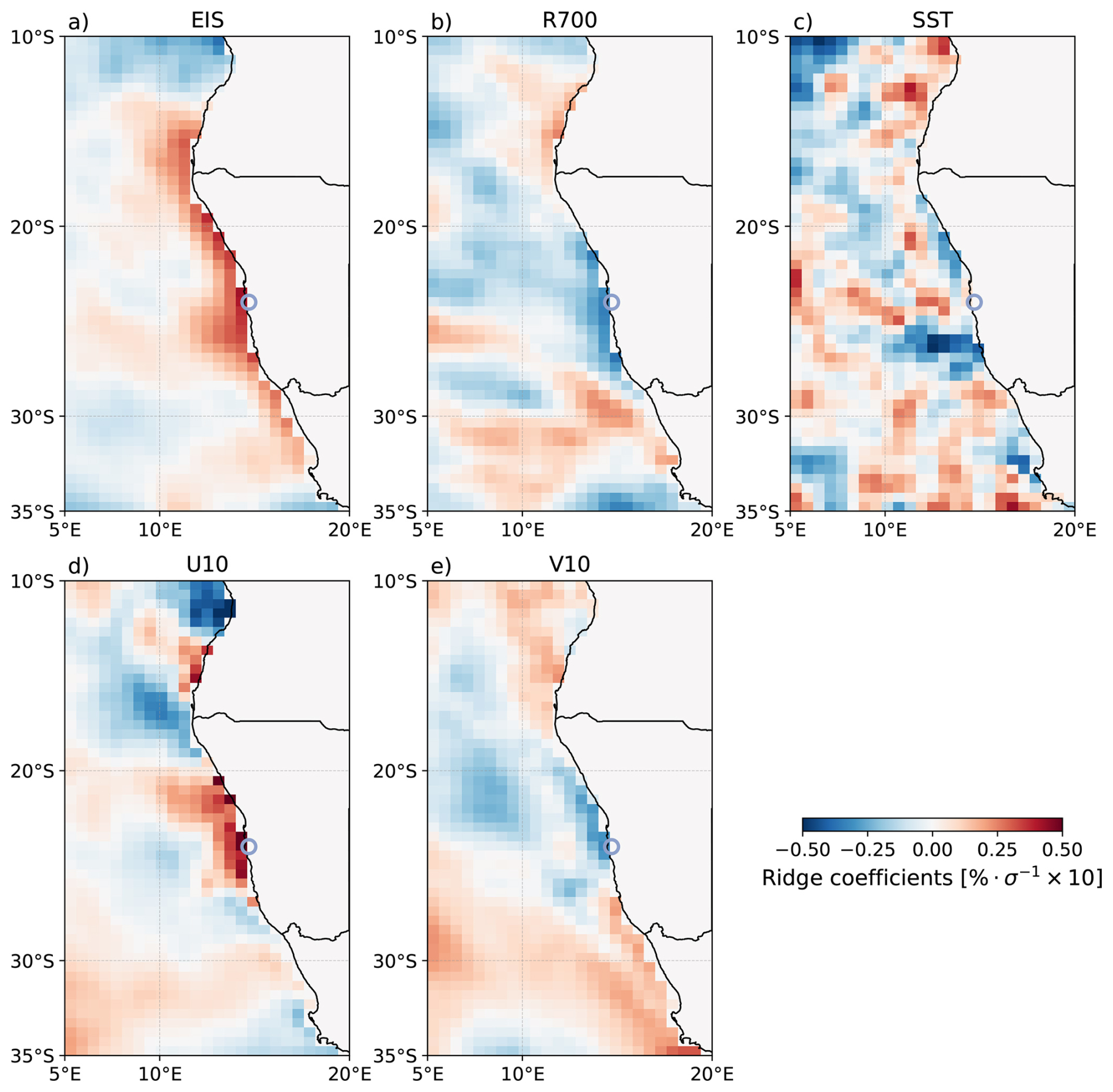
Figure 2 Sensitivity fields [% σ⁻¹], for each predictor in the CN-ERA5 configuration: (a) estimated inversion strength, (b) relative humidity at 700 hPa, (c) sea surface temperature, (d) 10 m eastward wind, and (e) 10 m northward wind. The blue circle indicates the center of the CN region.

For EIS (Fig. 2a), a positive pattern is evident along the coastline, indicating that a strengthened inversion layer is positively correlated with higher FLC cover. This is consistent with many studies showing that stronger inversions are associated with increased marine low cloud cover (Myers and Norris, 2016; Scott et al., 2020; Ceppi and Nowack, 2021). This effect is attributed to a shallower, more humid, and cloudier boundary layer resulting from reduced mixing (Bretherton et al., 2013).

For R700 (Fig. 2b), moderate but systematically negative sensitivities are evident around the CN region. Increased free-tropospheric humidity can reduce cloud-top radiative cooling, thereby decreasing the mixing of surface moisture with FLCs (Christensen et al., 2013; Bretherton et al., 2013). At the same time, higher free-tropospheric humidity can reduce entrainment drying, which moistens the boundary layer and enhances FLCs (Van der Dussen et al., 2015; Myers and Norris, 2016). However, in situations with very shallow and strong inversion layers, as typically found in this region, the effect of reduced cloud-top radiative cooling is likely dominant. This is consistent with Andersen et al. (2020), who found a significant free-tropospheric dry anomaly over the coastal region where FLCs form on fog days in the CN.

In the SST sensitivity field (Fig. 2c) the most prominent feature is a region of strong, localized negative sensitivities between approximately 25–28° S where the Lüderitz upwelling cell is located (Siddiqui et al., 2023). This is in line with the current understanding of the system, as FLCs in the region often form when warm and moist air masses travel over the cold upwelling waters (Olivier and Stockton, 1989; Cermak, 2012; Spirig et al., 2019; Andersen et al., 2020). As this model is trained specifically for the CN region, it is expected that the nearby Lüderitz upwelling cell dominates the sensitivity field. Further south upwind of the Lüderitz cell, sensitivities are positive and may reflect enhanced surface latent heat fluxes, increasing the moisture content of the marine boundary layer. This pattern may be influenced by the Agulhas leakage, which transports warm water from the Indian Ocean into the South Atlantic (Biastoch et al., 2024), locally warming the ocean surface and altering SST gradients, thereby affecting atmospheric moisture fluxes. A similar pattern was found in Andersen et al. (2020).

The U10 sensitivity field (Fig. 2d) exhibits a strong, localized positive pattern along the coastline. A positive U10 sensitivity can be understood as a positive association between eastward winds and FLC cover, which indicates the onshore advection of FLCs formed over the ocean, in agreement with Andersen et al. (2020).

Finally, for V10 (Fig. 2e), the sensitivities are weaker than those for U10, with negative values over the region itself and a broader band of positive values farther south. This structure appears in all four configurations and shifts northward in the AN region (See Appendix A), like the other sensitivity patterns. The positive area lies upwind of the region, where stronger southerly winds favour coastal upwelling and cooler SSTs, which in turn favour FLCs. The negative values over the region itself are consistent with Andersen et al. (2020), who found less pronounced coast-parallel winds on fog days in the CN, associated with synoptic-scale disturbances producing a northerly wind anomaly ahead of the trough that favours stratus formation and onshore advection.

Differences in model skill are also evident: the CN-ERA5 model presented here has a coefficient of determination of $R^{\mathrm{2}}=\mathrm{0.30}\pm \mathrm{0.26}$ (mean ± SD across the 6 cross-validation folds), while the AN-ERA5 (see Appendix A) model achieves $R^{\mathrm{2}}=\mathrm{0.38}\pm \mathrm{0.12}$. These R² values are consistent with those reported in other cloud-controlling factor framework studies (Scott et al., 2020; Andersen et al., 2022). Compared with CN, the AN sensitivity patterns are systematically shifted northward, toward the AN region: this applies to the EIS, R700, SST and wind sensitivities described above. In particular, for SST sensitivities, the strongly negative signal associated with the Lüderitz upwelling cell in the CN-ERA5 configuration is less pronounced in the AN-ERA5 configuration, while a broader region of negative sensitivities emerges farther north, centered on the Cape Frio upwelling cell.

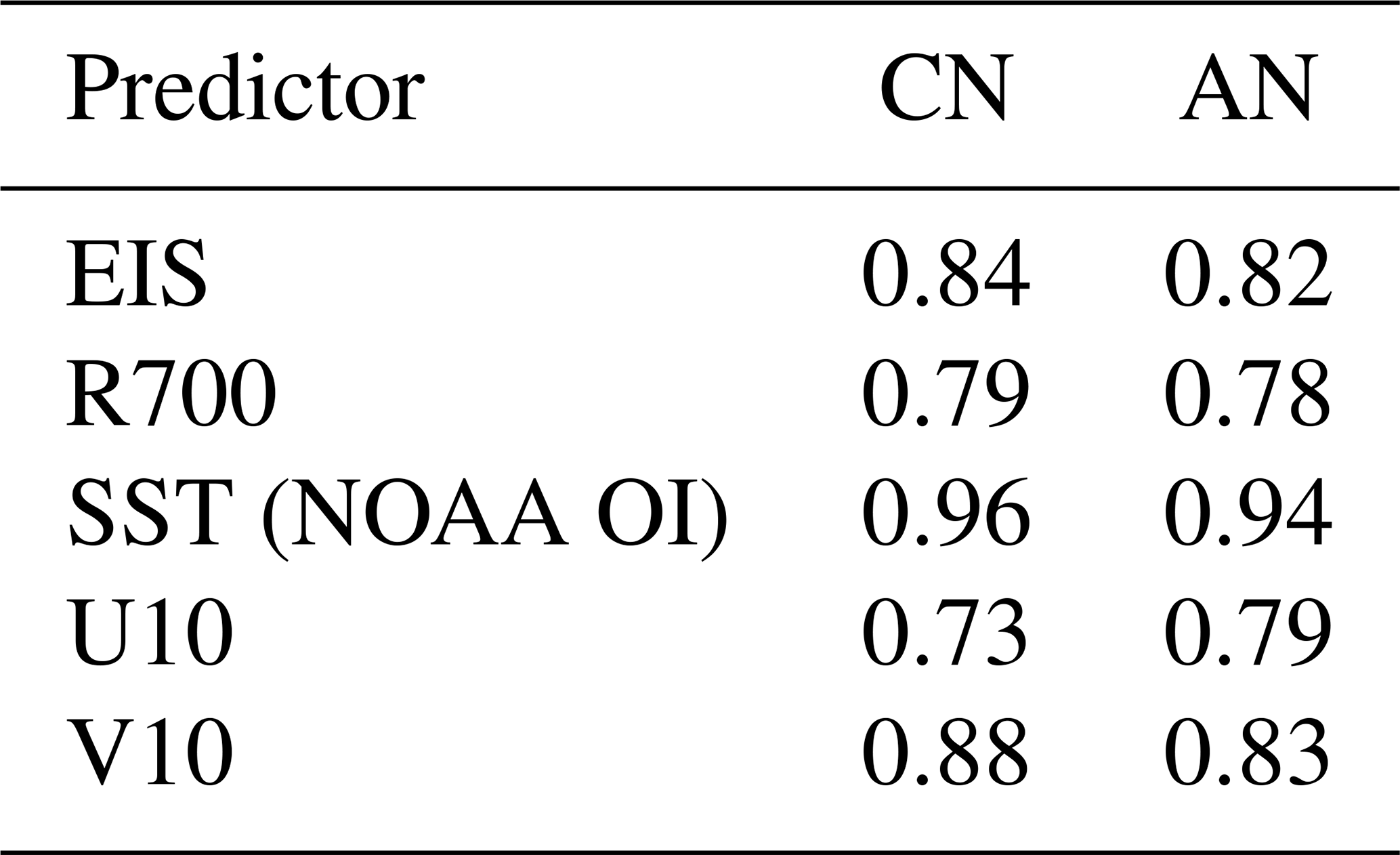
To test the extent to which sensitivities depend on the choice of reanalysis data set used, the MERRA-2 reanalysis was employed instead of ERA5 for the meteorological drivers. The resulting CN-MERRA-2 ($R^{\mathrm{2}}=\mathrm{0.31}\pm \mathrm{0.26}$) and AN-MERRA-2 ($R^{\mathrm{2}}=\mathrm{0.36}\pm \mathrm{0.09}$) sensitivity fields (see Appendix A) exhibit some localized differences but overall show the same patterns as the sensitivities of the ERA5 set. The spatial correlations (Pearson's r) between the ERA5 and MERRA-2 sets for each predictor are presented in Table 1. The highest correlations are observed for SST, which is expected since the SST data in both configurations are derived from NOAA OI.

Table 1 Spatial correlations (Pearson's r) between the sensitivity patterns derived from the ERA5 and MERRA-2 predictor sets.

While the AN model shows comparatively stable out-of-sample skill across folds, the CN model exhibits substantially greater fold-to-fold variability in both the ERA5 and MERRA-2 configurations. Two of the six folds, covering July 2009 to August 2014, consistently show near-zero predictive skill regardless of the reanalysis product, coinciding with a period of reduced variance in the observed CN FLC anomalies. The model's absolute error in these folds does not decrease proportionally with the reduced target variability, suggesting a reduced ability to resolve lower-amplitude fluctuations in FLC cover, in addition to the mechanical effect of reduced variance on R².

Overall, these sensitivities are consistent with the guiding hypothesis: the positive sensitivities to coastal EIS, the localized but negative sensitivities to SST, and the strong influence of the onshore circulation indicate that FLCs in the region are predominantly advective in nature.

3.2 Historical reconstructions of Namib FLCs

The historical FLC cover reconstructions are shown in Fig. 3 for the AN (Fig. 3a) and CN (Fig. 3b) regions, with the ERA5 configuration in brown and the MERRA-2 configuration in green. Shaded areas indicate the observational period (see Sect. 2.1). The reconstructions are obtained by applying the sensitivities estimated via ridge regression to the corresponding controlling-factor anomalies following Eq. (3). The final reconstruction uses fold-averaged sensitivities, in which each month from 2004–2019 contributes to the training data in all but one of the six cross-validation folds, making the resulting reconstruction non-independent. A fully out-of-sample reconstruction can be obtained by combining the predictions from all test folds, yielding correlations with the observations of r=0.64 for AN-ERA5, r=0.62 for AN-MERRA-2, r=0.61 for CN-ERA5, and r=0.63 for CN-MERRA-2 (see Fig. B1). This approach, however, introduces a discontinuity at the start of the observational period (2004). Using fold-averaged sensitivities ensures a continuous time series from 1982 to 2019, which allows the analysis of interannual variability and long-term trends. Averaging the monthly FLC cover anomalies to annual values slightly decreases the correlation with observations (r=0.66–0.68 monthly vs. r=0.61–0.64 annual, across regions and reanalyses).

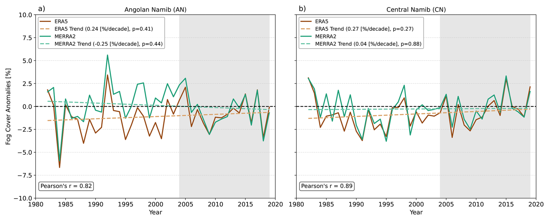
Figure 3 Historical reconstructions (1982–2019) of interannual FLC cover anomalies for AN (a) and CN (b). The ERA5 configuration is shown with a solid brown line, and MERRA-2 with a solid green line, while the linear trends are indicated by dashed lines. The shaded area highlights the observational period (2004–2019).

To better characterize these annual anomalies, we examine which months they are primarily associated with and whether they reflect changes in the intensity of the fog season or shifts in its timing or duration. Using the satellite-observed FLC record (2004–2019), we correlated each calendar month's FLC anomaly with the annual mean anomaly across all years to identify which months' variability is most closely linked to the overall annual signal (Fig. B2). In AN, significant positive correlations occur in several months, with the strongest relationships found in June and July, when the fog season is still developing toward its maximum. In contrast, August and September, despite having the highest climatological fog occurrence, show weaker relationships with the annual anomaly. This indicates that AN annual anomalies are primarily associated with variability during the early development of the fog season, potentially reflecting changes in the strength and/or timing of seasonal build-up rather than substantial changes in season duration. In CN, where fog occurs throughout the year with a weaker seasonal cycle, annual anomalies are most strongly associated with variability outside the climatological peak season, particularly in January, March, and April, while the peak period contributes comparatively little to interannual variability.

The reconstructions in both regions show strong correlations between the ERA5 and MERRA-2 setups (r=0.82 in AN and r=0.89 in CN). In the AN, both sets capture similar year-to-year fluctuations, including a peak in 1992 and a pronounced negative anomaly in 1984. However, a noticeable bias exists between the two configurations in the AN: the ERA5 set is systematically about 2 % lower than the MERRA-2 set, producing opposite signs in the reconstructed trends (dashed lines: 0.24 % per decade for ERA5 and −0.25 % per decade for MERRA-2). In contrast, in the CN, no consistent bias is observed, and both reconstructions are closer, yielding positive trends (0.27 % per decade for ERA5 and 0.04 % per decade for MERRA-2). However, these trends are not statistically significant and therefore cannot be distinguished from near-zero trends. As expected, due to the non-independent data, both sets exhibit very similar behavior during the observation period. Overall, despite the presence of a climate change signal over these 40 years, notably the warming of SSTs in this region (Tomety et al., 2024), the near-zero linear trends across all reconstructions highlight the stability of the system. However, this contrasts with Li et al. (2025), where in-situ fog water measurements show a decline in fog amount after 1996. These measurements are from Gobabeb, which, although within the latitudinal band of the CN region, lies some 60 km inland and therefore outside the study domain, which is restricted to the coastal strip within 24 km of the coastline. No corresponding break point is found in the reconstructed FLC cover time series, though the reconstruction carries substantial uncertainty. A change observed at Gobabeb, an inland site outside the study domain, would not necessarily be expected to emerge in this regional-average coastal reconstruction. Their record is also not a single continuous measurement, but a series assembled from successive fog collectors operating on different measurement principles. The 1996 step coincides with one of these instrument transitions, which calls for care in interpreting the break point.

To further investigate reasons behind the reconstructed FLC cover trends, the total reconstructions are decomposed into the partial contributions of the individual predictors. The long-term linear trend contributions are then calculated and presented as bar plots in Fig. 4, where “Total” represents the reconstructed trends from Fig. 3. This decomposition shows how much each cloud-controlling factor contributes to the reconstructed trends, and whether their contributions reinforce or offset one another. As seen in Fig. 3, the total trends are not statistically significant. However, several CCFs have significant trend contributions, as indicated by the red stars. Note that the relative magnitude of each predictor's contribution shown in Fig. 4 depends on the ridge-regression sensitivities, which are estimated jointly across all predictors under the shared l²-norm regularization term and are therefore shaped by the collinearity structure among predictors. Consequently, a difference between reanalyses in a given predictor's contribution should not, on its own, be taken as evidence of a difference in that variable's underlying physical importance.

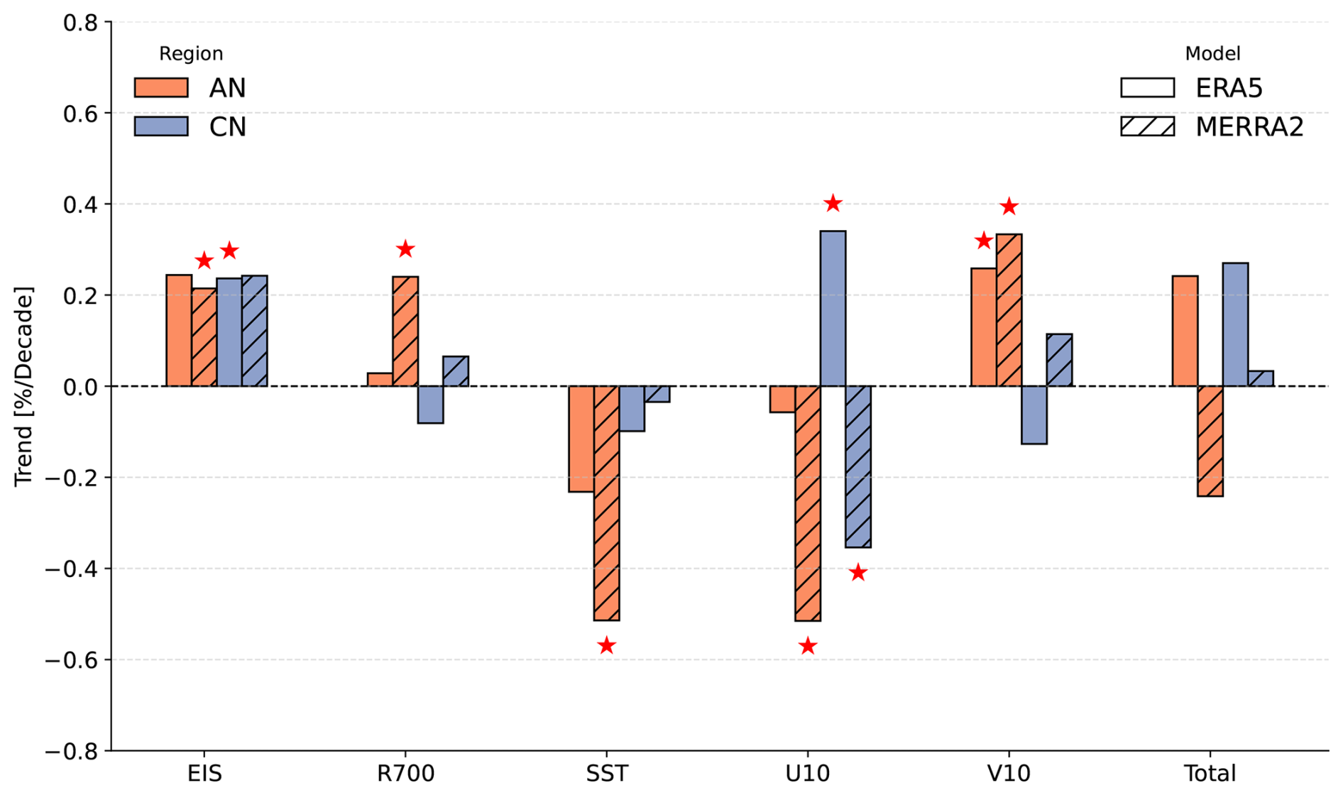
Figure 4 Yearly FLC cover anomaly linear trend coefficients (1982–2019) showing the partial contribution of each cloud-controlling factor to the total historical reconstruction. The AN region is shown in orange and the CN region in blue. ERA5 is represented by solid bars and MERRA-2 by dashed bars. Red stars indicate statistically significant trends (p<0.05).

In addition, Fig. 5 presents the spatial trends of the predictors derived from the ERA5 and MERRA-2 reanalysis and the NOAA OI SST dataset. Because the mean states are of interest here, the trends are derived directly from the raw reanalysis data, without deseasonalization or the standard scaling applied in the statistical model. For this reason, these maps cannot be directly linked to the coefficient maps shown in Fig. 2. Difference maps are shown in Fig. B3 in Appendix B.

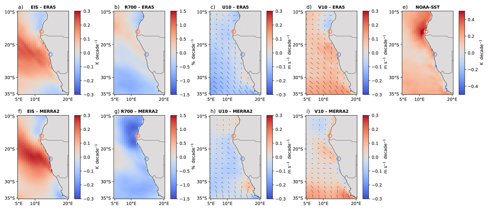
Figure 5 Spatial decadal trends over 1982–2019 for ERA5 (a–d) and MERRA-2 (f–i). Panels show EIS [K per decade] (a, f), R700 [% per decade] (b, g), U10 [m s⁻¹ per decade] (c, h), V10 [m s⁻¹ per decade] (d, i), and NOAA OI SST [K per decade] (e). Arrows in panels (c), (d), (h), and (i) indicate wind speed and direction. The centers of the two study regions are marked by circles: Angolan Namib (AN) in orange and Central Namib (CN) in blue.

For EIS, in both regions and for both configurations, positive trend contributions of around 0.2 % per decade are observed (Fig. 4). Only CN-ERA5 and AN-MERRA-2 show a statistically significant trend contribution, whereas CN-MERRA-2, despite a slightly larger trend contribution, is not significant (p=0.1) due to higher variability in the EIS data. The EIS trends (Fig. 5a and f) are in good agreement between ERA5 and MERRA-2, showing an increasing inversion strength along the Namibian coastline. This enhanced atmospheric stability contributed to the increase in FLC cover anomalies in the CN.

For R700, only AN-MERRA-2 shows a significant trend of 0.23 % per decade (Fig. 4). The R700 trends in Fig. 5b and g differ between ERA5 and MERRA-2: ERA5 shows a positive trend in the northern part of the ocean, whereas MERRA-2 exhibits a strong negative trend. Despite these differences, in both reanalyses the AN is located in a region of negative trends, indicating that a drier free troposphere contributes to the increase of FLC anomalies in the AN.

Changes in SST lead to relatively strong negative trend contributions in the AN for both configurations (Fig. 4), with a significant trend of −0.51 % per decade for AN-MERRA-2, where local SST trends are most pronounced (see Fig. 5e). For CN, both configurations show small, non-significant negative trends.

As detailed in Sect. 2.2, the U10 and V10 fields were masked over land prior to their use as predictors. This choice is supported by the comparison between the ERA5 and MERRA-2 wind fields: good agreement between the two reanalyses is expected over the ocean, as the fields are relatively smooth there. Even when observational data are sparse, the flow is predictable, allowing the reanalysis models to achieve high precision. Over land, however, complex topography introduces heterogeneity, which can be further amplified by differences in model parameterizations. This pattern is consistent with previous studies (Brune et al., 2021). To evaluate which reanalysis dataset better represents the observed conditions, we compared the seasonally averaged diurnal wind direction cycle for 2016 from the FogNet station at Marble Koppie (22.97° S, 14.99° E) (Kaspar et al., 2015) with the corresponding data from ERA5 and MERRA-2. Figures B4 and B5 in Appendix B show that both reanalyses reproduce the observed diurnal and seasonal wind regime at this site, including the seasonal reversal between the predominantly westerly summer flow and the easterly winter flow, indicating that the thermo-topographic circulation of the region (Lindesay and Tyson, 1990) is broadly captured. Differences remain in the directional distribution of the flow, and these are more pronounced in MERRA-2, which concentrates the wind into a narrower sector than observed and underrepresents the northwesterly sector in DJF and SON. ERA5 is closer to the observations in both respects, consistent with its finer spatial resolution. A comparison at a single inland station over one year does not permit a general assessment of reanalysis wind fields over the coastal plain, and comparative studies of ERA5 and MERRA-2 in this region are warranted. For this reason, and because oceanic wind fields show much better agreement between the two reanalyses, we consider the masked (ocean-only) U10 and V10 fields to be more reliable predictors.

Finally, U10 and V10 lead to strong trend contributions (Fig. 4). Across three of the four configurations, a consistent pattern emerges: U10 contributions are negative or near-zero, while V10 contributions are positive. This holds for AN-MERRA-2 ($\text{U10}=-\mathrm{0.52}$ % per decade, significant; V10=0.33 % per decade, significant), CN-MERRA-2 ($\text{U10}=-\mathrm{0.35}$ % per decade, significant; V10 positive, non-significant), and AN-ERA5 (U10 near-zero, non-significant; V10=0.26 % per decade, significant). CN-ERA5 stands out as the exception, showing the opposite sign pattern: a significant positive U10 contribution (0.34 % per decade) together with a negative, non-significant V10 contribution. This sign difference in CN-ERA5 can potentially be explained by the U10 sensitivity field (Fig. 2d): a negative sensitivity area just north of the region along the coast, transitioning sharply to a positive sensitivity closer to the region, is present in all four configurations (see Appendix A), but this transition is sharper and more intense in CN-ERA5 than in the other three. Because U10 and V10 are correlated predictors, this distinct U10 pattern may also be linked to the corresponding difference in the V10 trend contribution for CN-ERA5.

Due to remaining discrepancies between the two reanalysis products over near-coastal ocean areas, the wind trend contributions should still be interpreted with some caution. However, for the other predictors, Fig. 4 highlights a key feature of the system: the near-zero trends in FLC cover in the historical reconstructions arise from a balance between opposing mechanisms. On one side, increased atmospheric stability leads to an increase in FLC cover; on the other, SST warming drives a decrease. Whether this balance persists or is eventually disrupted under more extreme forcing remains a critical question for anticipating the future evolution of FLCs in the region.

3.3 Influence of SST on interannual FLC variability

In the previous sections, the sensitivities obtained through the statistical learning framework are analyzed and subsequently used to create historical reconstructions of FLC cover anomalies. The derived trends were found to be unreliable, notably because of discrepancies between ERA5 and MERRA-2, as well as a general lack of statistical significance in the estimated trends. However, the reconstructed interannual FLC variability agrees relatively well with the observations. For this reason, we detrend the reconstructions, which leads to a small increase in the correlations between the ERA5 and MERRA-2 setups in the AN (r=0.86 in AN and r=0.90 in CN; not shown). These detrended reconstructions are then used to further examine the influence of SSTs on interannual FLC variability. Figure 6 shows the detrended 3-month running mean FLC cover anomalies for the 1982–2019 period in the ERA5 configuration, compared with the Oceanic Niño Index (ONI), which characterizes ENSO phases in the Pacific, for the AN (Fig. 6a) and CN (Fig. 6c) regions. The corresponding scatter plots (Fig. 6b and d) show that warm and cool ENSO phases overlap substantially in FLC anomaly, consistent with the weak overall relationship. Figure 6e displays the Pearson correlation coefficients as a function of monthly time lag, illustrating the effects of temporal delay. Peak correlations are observed at time lags of two months in the CN region and five months in the AN region. These maximum values (r=0.24 for AN–ERA5 and r=0.21 for CN–ERA5; r=0.23 for AN–MERRA-2 and r=0.21 for CN–MERRA-2; see Fig. C1) are consistent with Rouault and Tomety (2022), who reported significant correlations between ENSO and Benguela upwelling SST with lags of up to eight months. Importantly, they find opposite signs for the northern and southern Benguela: in the northern Benguela, which broadly covers both of our study regions, El Niño is associated with an enhancement of the upwelling-favorable trade winds and thus stronger upwelling and cooler coastal SST. Taking into account Fig. 6 and the findings of Rouault and Tomety (2022), ENSO appears to slightly enhance FLCs in the region, at least partially through its effect on local winds.

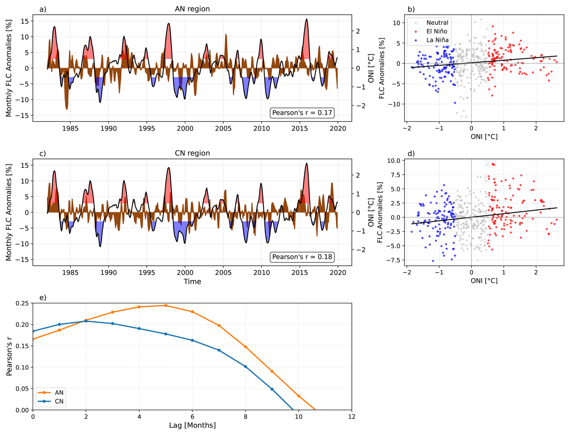
Figure 6 Detrended 3-month running mean FLC cover anomalies compared with the Oceanic Niño Index (ONI) during 1982–2019 for: AN-ERA5 (a) and CN-ERA5 (c). FLC anomalies are brown and ONI black, with warm ($\ge +\mathrm{0.5}\mathrm{°}\mathrm{C}$) and cool ($\le -\mathrm{0.5}\mathrm{°}\mathrm{C}$) phases highlighted in red and blue. (b, d) Corresponding scatter plots of FLC anomalies against the ONI, with points coloured by phase (red: warm; blue: cool; grey: neutral) and the least-squares fit in black. (e) Pearson correlation coefficients (r) between lagged FLC anomalies and ONI as a function of monthly lag for AN (orange) and CN (blue).

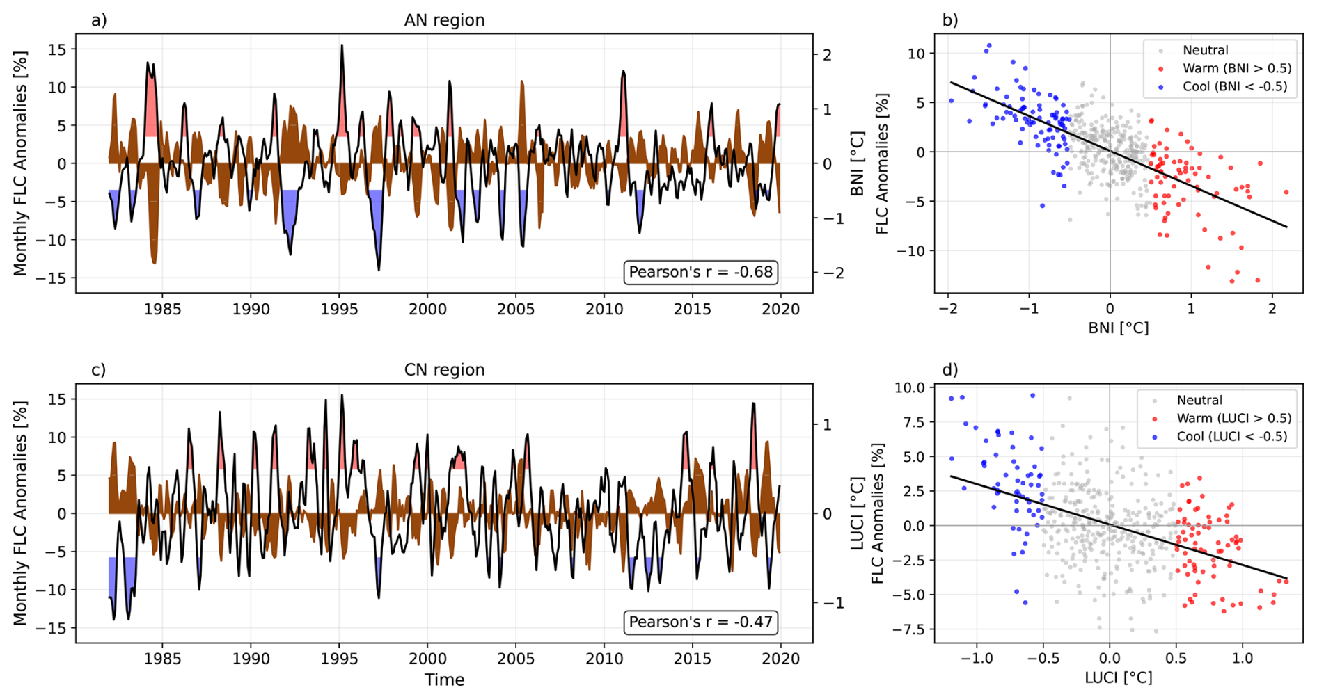
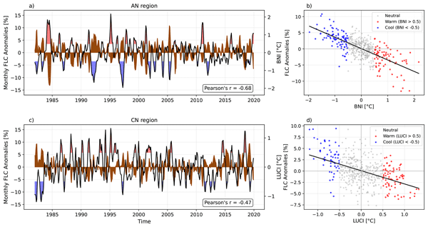
Figure 7 Detrended 3-month running mean FLC cover anomalies in the ERA5 setup during 1982–2019, compared with the Benguela Niño Index (BNI) for the AN region (a) and the Lüderitz Upwelling Cell Index (LUCI) for the CN region (c). FLC anomalies are shown in brown, and BNI/LUCI in black, with warm ($\ge +\mathrm{0.5}\mathrm{°}\mathrm{C}$) and cool ($\le -\mathrm{0.5}\mathrm{°}\mathrm{C}$) phases highlighted in red and blue, respectively. (b, d) Corresponding scatter plots of FLC anomalies against the respective index, with points coloured by phase (red: warm; blue: cool; grey: neutral) and the least-squares fit in black.

Although ENSO influences FLCs in the region, a stronger impact from local SST variability can be anticipated, notably from regional warming events known as Benguela Niño events. These events result from weakened trade winds, which promote the intrusion of warm tropical waters from the north and reduce coastal upwelling (Florenchie et al., 2003, 2004; Rouault et al., 2018). In addition, equatorially generated Kelvin waves can propagate along the African coast, causing the thermocline to deepen and surface waters to warm (Florenchie et al., 2003; Richter et al., 2010; Imbol Koungue et al., 2019). Rouault and Tomety (2022) further report that La Niña conditions favour the development of Benguela Niños in Angola and Namibia, providing a link between the two modes of variability. The Benguela Niño events are quantified, similarly to the ONI in the Pacific, using the Benguela Niño Index (BNI) (Shannon et al., 1986), which represents detrended SST anomalies averaged over 10–20° S and 8–14° E. The BNI region coincides with one of the strongest SST gradients on the planet (Brandt et al., 2024), spanning from the warm Angolan waters in the north to the cold upwelled Namibian waters in the south (see Fig. 1). Because SSTs play a key role in the Namibian FLC system, a correlation between the BNI and FLC cover can reasonably be expected. The BNI appears particularly suited for the AN region because it encompasses the Cape Frio upwelling cell, but it does not include information from the Lüderitz upwelling cell, which is especially relevant for the CN. To address this, we define the Lüderitz Upwelling Cell Index (LUCI) in a manner similar to the BNI, but for the region 24–28° S, 12–15° E, which encompasses this upwelling cell and has been identified by Siddiqui et al. (2023) as the Lüderitz upwelling region. BNI and LUCI vary primarily on multi-month timescales. Major Benguela Niño events typically persist for six months or longer, with some events lasting close to a full year (Shannon et al., 1986). The Lüderitz upwelling cell relevant to the LUCI index persists year-round, with intensity generally weaker in winter and spring (Andrews and Hutchings, 1980; Hutchings et al., 2009). The robustness of the BNI and LUCI definitions to their exact spatial extent was assessed by testing the sensitivity of their correlation with the respective reconstructions to shifts in the defining box location (Appendix C, Fig. C3). BNI shows stable correlation for small shifts, weakening only for large shifts, consistent with its broad, literature-defined extent within a strong regional SST gradient. LUCI shows a slight increase in correlation for a northward shift. The Lüderitz cell itself is fixed in location, but upwelling is not confined to it: the coastal upwelling band extending north towards the CN region also matters for FLC variability there, and a northward shift captures it. The increase therefore reflects the broader coastal upwelling signal rather than a stronger Lüderitz-specific relationship.

Figure 7 shows the detrended 3-month running mean FLC cover anomalies for 1982–2019 in the ERA5 configuration, superposed with the BNI for the AN region (Fig. 7a) and with LUCI for the CN region (Fig. 7c). A strong negative correlation is observed between FLC cover anomalies and the BNI in the AN region, with a Pearson's $r=-\mathrm{0.68}$ (AN-MERRA-2: $r=-\mathrm{0.68}$; see Fig. C2). Using the coefficients of determination (R²=0.46), it becomes apparent that the BNI explains nearly half of the interannual FLC variability in the AN. For example, in 1984, the most prominent negative FLC anomaly in the AN appears to have been largely driven by a particularly pronounced warm water intrusion, as captured by the BNI. In the CN, a moderate negative correlation exists between FLC anomalies and LUCI. Although weaker than the FLC–BNI correlations in the AN, LUCI is able to explain 22 % (R²=0.22) of the interannual FLC variability in the CN. It is important to remember that these two indices, BNI and LUCI, are related to different mechanisms: BNI primarily reflects the intrusion of warm equatorial waters due to weakened trade winds, whereas LUCI is specifically designed to capture variability in the Lüderitz upwelling cell. However, LUCI and BNI are not entirely independent: the intrusion of tropical warm waters probably also affects the LUCI region. The AN region, being closer to the source is more strongly affected, whereas the warming is less intense by the time it reaches the CN region.

One important limitation should be noted when correlating the historical reconstructions with the BNI and LUCI indices. The statistical model uses SST anomalies as predictors, and the BNI and LUCI indices represent SST anomalies over subregions of this domain. We therefore computed the correlations between the BNI and LUCI indices and the observed FLC anomalies over the corresponding subregions during 2004–2019. These correlations are lower than those obtained from the model-predicted FLC cover, decreasing by approximately 20 % for AN and 30 % for CN (not shown). This decrease likely reflects the non-independence of the indices and predictors; however, the shorter observational period may also contribute to the reduced correlations. Despite the decrease, the correlations remain statistically significant (p<0.05) and indicate that physically relevant relationships exist between regional SST anomalies and FLC cover.

4 Conclusions and outlook

Fog and low clouds are the main source of moisture sustaining ecosystems across the hyper-arid Namib, so identifying the mechanisms governing their variability matters for anticipating how this moisture supply may change under future climate conditions. The main goals of this study were to explain and quantify the key large-scale meteorological factors controlling fog and low clouds (FLC) in the Namib region, and to assess the relevance of SST pattern variability on interannual FLC cover. We focused on two subregions characterized by most frequent FLC occurrence: the Angolan Namib and the Central Namib. To achieve this, we applied a cloud-controlling factor analysis (Klein et al., 2017; Scott et al., 2020; Ceppi and Nowack, 2021; Andersen et al., 2023) using ridge regression to predict monthly FLC cover anomalies. The main findings of this study are:

1. Estimated inversion strength (EIS), relative humidity at 700 hPa (R700), sea surface temperature (SST), and the eastward and northward components of the 10 m wind (U10 and V10, respectively) were used as the five key factors controlling FLC cover in the region. The derived model sensitivities quantify the large-scale meteorological mechanisms that lead to FLC occurrence in the Namib: a strong inversion along the coast underneath a dry free troposphere, onshore advection of the marine boundary layer air, and, in the case of the CN, pronounced upwelling at the Lüderitz upwelling cell. These findings are consistent with prior studies (Olivier and Stockton, 1989; Seely and Henschel, 1998; Spirig et al., 2019; Formenti et al., 2019; Andersen et al., 2019, 2020), and the estimated sensitivities further support the advective nature of FLCs in the Namib region, in agreement with our first guiding hypothesis.

2. The derived sensitivities were then used to reconstruct historical FLC cover anomalies for the period 1982–2019. These reconstructions show moderate agreement with observations, with correlation coefficients between r=0.61 and r=0.64 across all regions and reanalysis datasets. Trend analysis of the reconstructed FLC cover reveals near-zero trends, resulting from opposing mechanisms: increased atmospheric stability that favors FLCs is counterbalanced by warming sea surface temperatures, which tend to reduce FLCs.

3. Using two reanalysis datasets, ERA5 and MERRA-2, revealed discrepancies between them, largest in the near-surface wind fields over land. At the Marble Koppie station, both reproduce the observed diurnal and seasonal wind regime, including the seasonal reversal between the westerly summer flow and the easterly winter flow, indicating that the thermo-topographic circulation of the region (Lindesay and Tyson, 1990) is broadly captured. Differences remain in the directional distribution of the flow and are more pronounced in MERRA-2, with ERA5 closer to the observations, consistent with its finer spatial resolution. This highlights the need for comparative studies of the two reanalyses in the area.

4. ENSO was found to have a weak influence on FLCs in the Namib, with El Niño conditions slightly enhancing FLC cover at lags of two to five months. This is consistent with the lagged ENSO influence on Benguela upwelling reported by Rouault and Tomety (2022). However, local SST dynamics are shown to be more important for FLCs in the Namib.

5. Benguela Niño warm SST anomalies, associated with the intrusion of tropical waters, explain nearly half (R²=0.46) of the interannual FLC variability in the Angolan Namib region, while the Lüderitz upwelling cell accounts for 22 % (R²=0.22) of the variability in the Central Namib region. This emphasizes the role of coastal upwelling and tropical warm water intrusions as key drivers of fog variability along the southwestern African coast.

More broadly, this study shows that a cloud-controlling factor framework, developed for marine low clouds, can be applied to a coastal fog system and yield physically interpretable sensitivities. Extending the analysis to spatial predictor fields is what allows non-local influences such as upwelling cells upwind of the study regions to be captured. The resulting reconstruction extends the 16-year satellite record to nearly four decades, which is what makes the link between FLC variability and regional climate modes accessible in the first place.

Future changes in coastal upwelling and tropical warm water intrusions in the BNI region have important implications for fog response and may be key to producing robust estimates of fog in the Namib Desert. The framework developed here could be applied to climate model output to test whether the compensation between increased atmospheric stability and SST warming identified in Sect. 3.2, which currently keeps the historical FLC trend near zero, persists under stronger future forcing or is eventually disrupted.

Appendix A: Sensitivities of alternative configurations

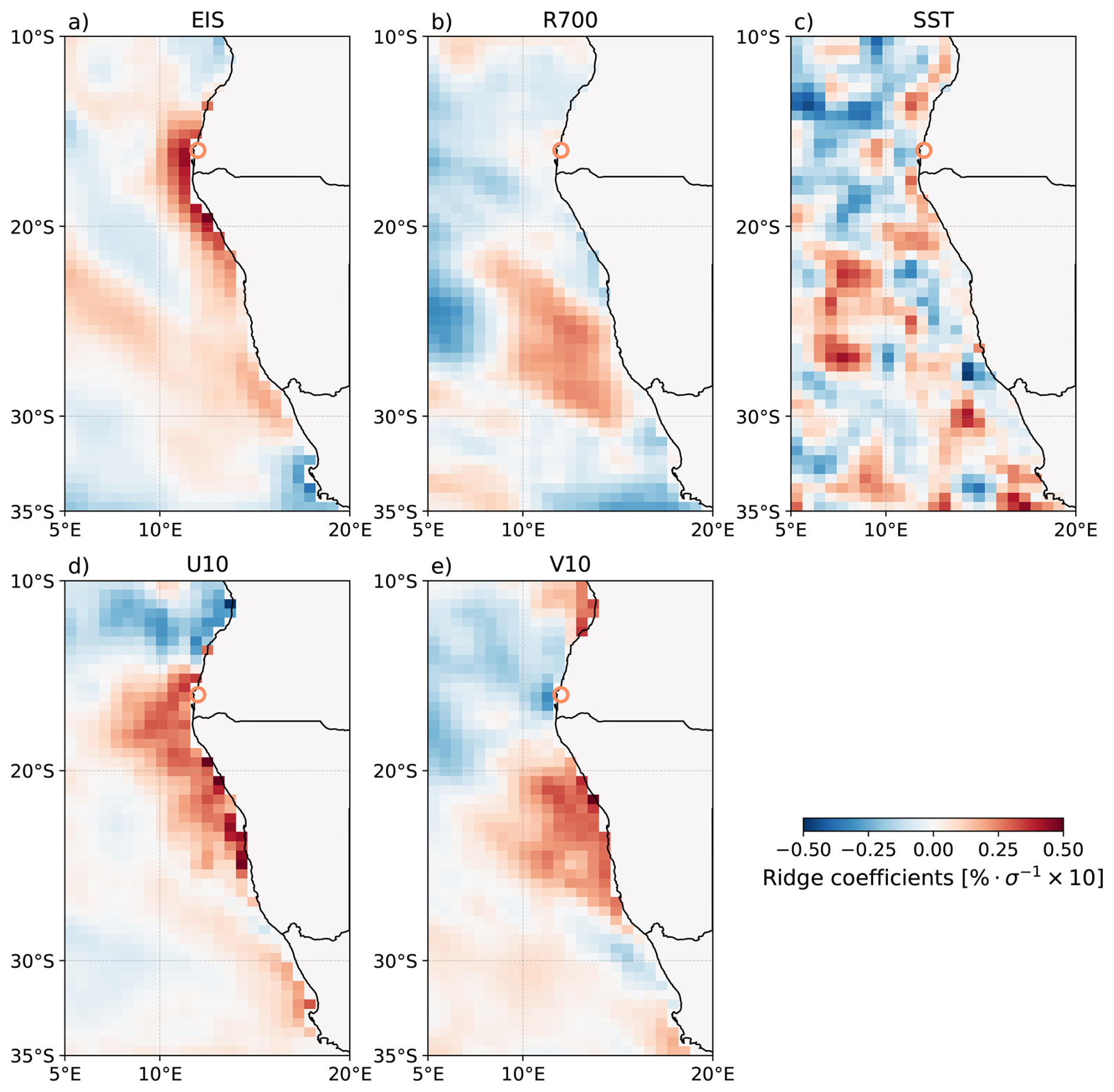
Figure A1 Sensitivity fields [% σ⁻¹], for each predictor in the AN-ERA5 configuration: (a) estimated inversion strength, (b) relative humidity at 700 hPa, (c) sea surface temperature, (d) 10 m eastward wind, and (e) 10 m northward wind. The orange circle indicates the center of the AN region.

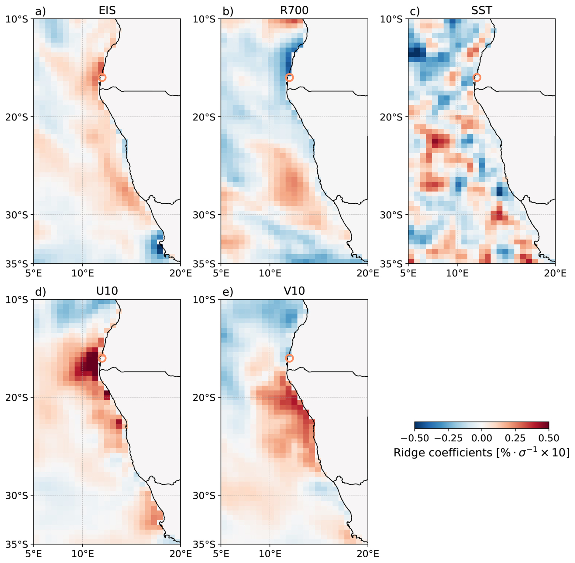
Figure A2 Sensitivity fields [% σ⁻¹], for each predictor in the AN-MERRA-2 configuration: (a) estimated inversion strength, (b) relative humidity at 700 hPa, (c) sea surface temperature, (d) 10 m eastward wind, and (e) 10 m northward wind. The orange circle indicates the center of the AN region.

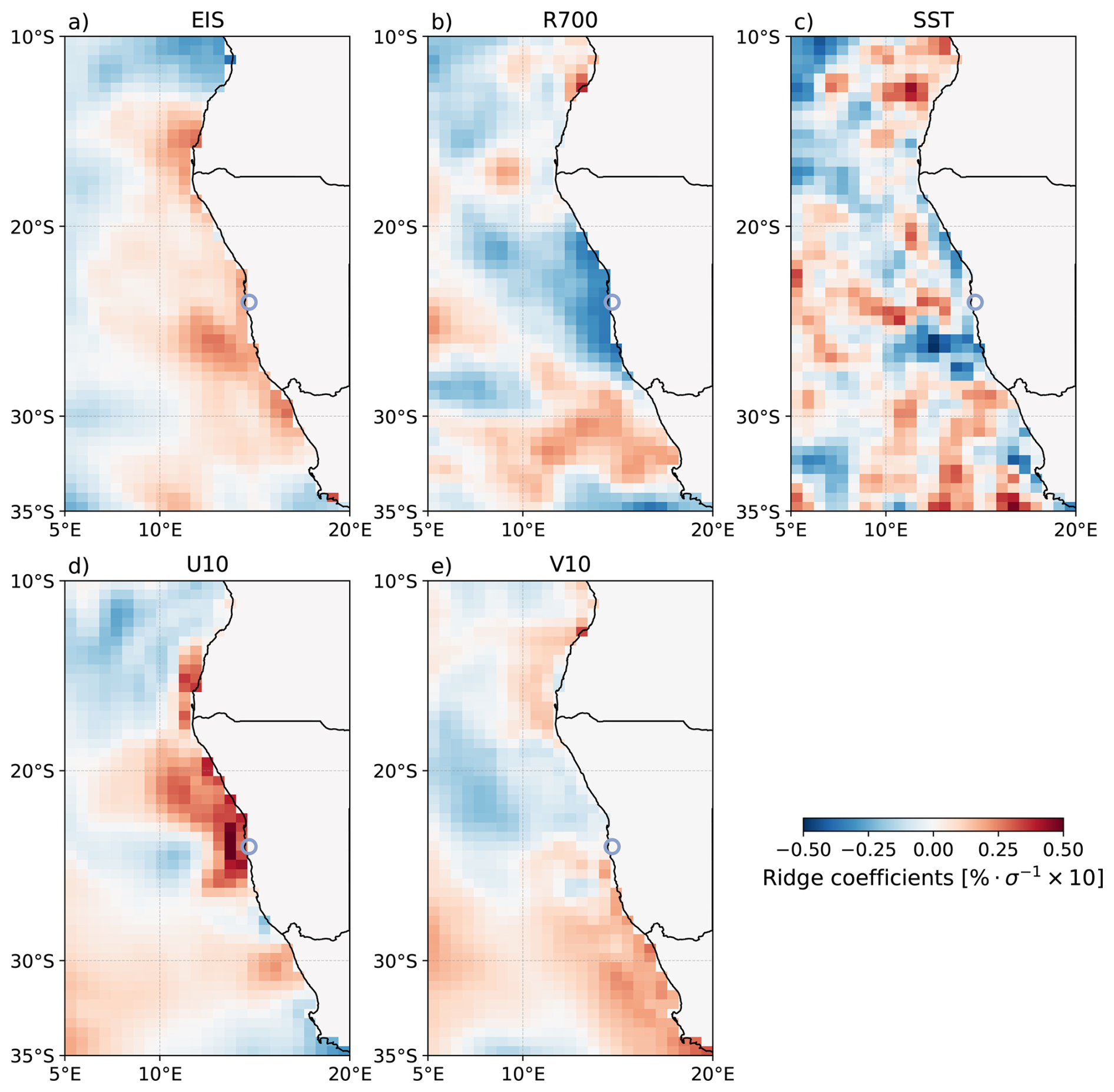
Figure A3 Sensitivity fields [% σ⁻¹], for each predictor in the CN-MERRA-2 configuration: (a) estimated inversion strength, (b) relative humidity at 700 hPa, (c) sea surface temperature, (d) 10 m eastward wind, and (e) 10 m northward wind. The blue circle indicates the center of the CN region.

Appendix B: ERA5 and MERRA-2 comparisons

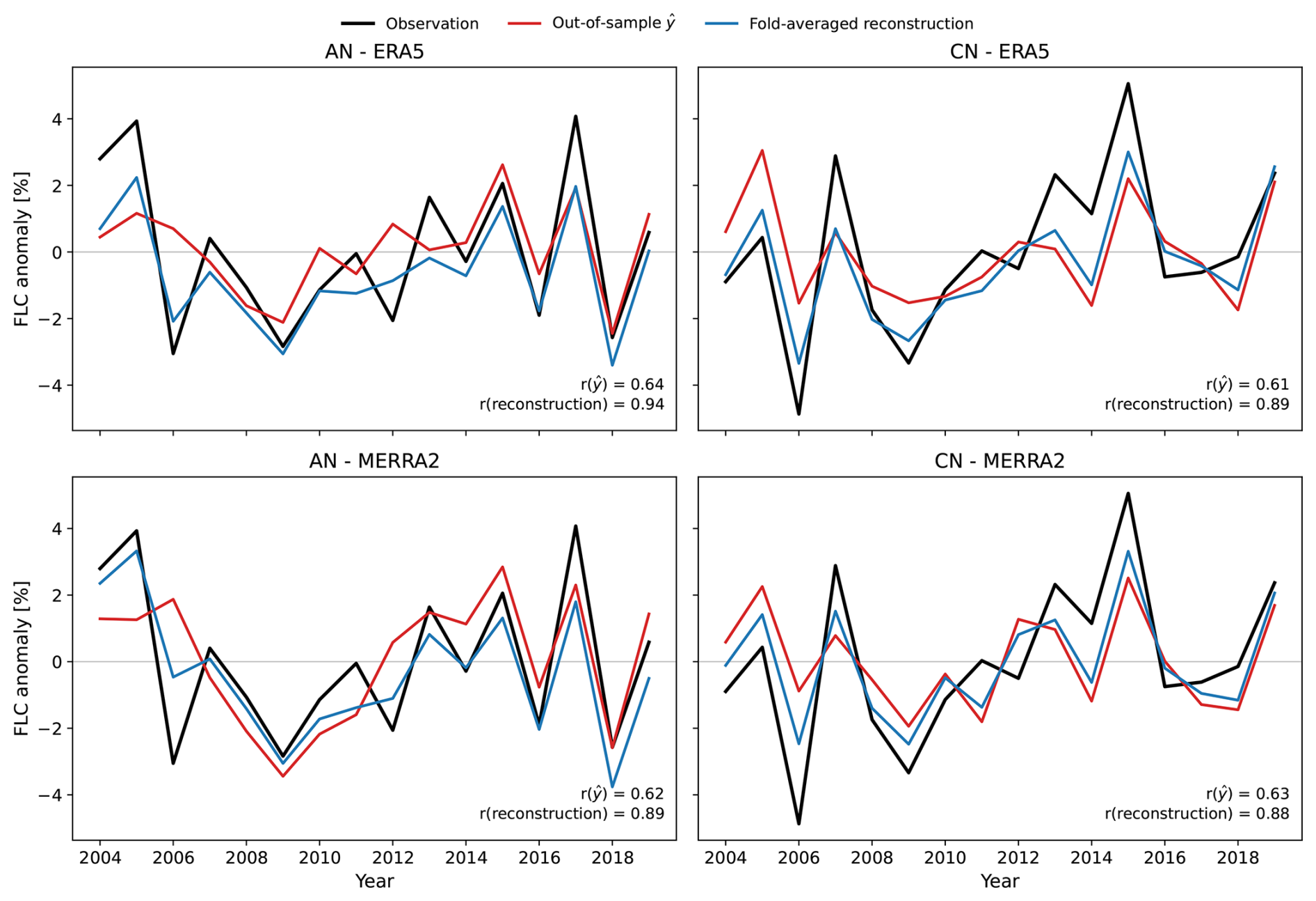
Figure B1 Comparison of observed annual FLC anomalies against the fully out-of-sample prediction ($\widehat{y}$, red) and the fold-averaged reconstruction used in Fig. 3 (blue), for each region and reanalysis. The fold-averaged reconstruction is not independent of the observations and correlates more closely with them than the genuinely out-of-sample prediction, illustrating why Fig. 3 does not overlay observations directly.

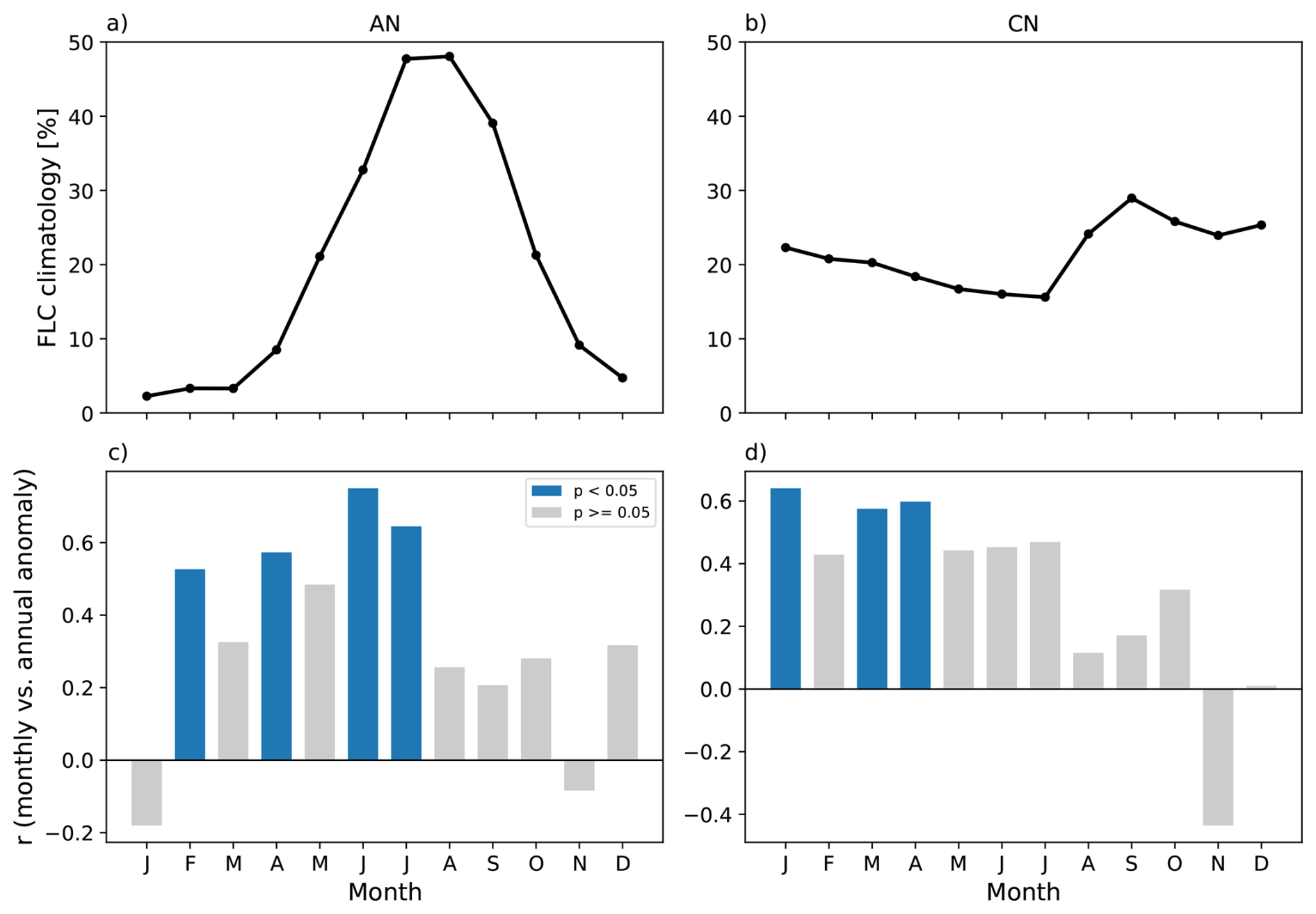
Figure B2 Based on the satellite-observed FLC record (2004–2019). (a, b) Average monthly cycle of FLC cover for AN and CN. (c, d) Correlation (r) between each month's FLC anomaly and the annual mean anomaly, for AN and CN; blue bars indicate p<0.05.

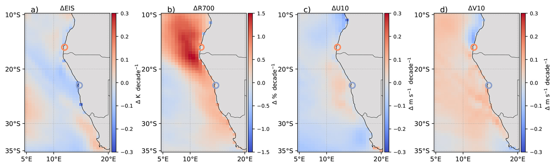
Figure B3 Spatial decadal trend differences between ERA5 and MERRA-2 ($\mathrm{\Delta }=\text{ERA5}-\text{MERRA-2}$) over 1982–2019 for (a) ΔEIS, (b) ΔR700, (c) ΔU10, and (d) ΔV10. The centers of the two study regions are marked by circles: Angolan Namib (AN) in orange and Central Namib (CN) in blue.

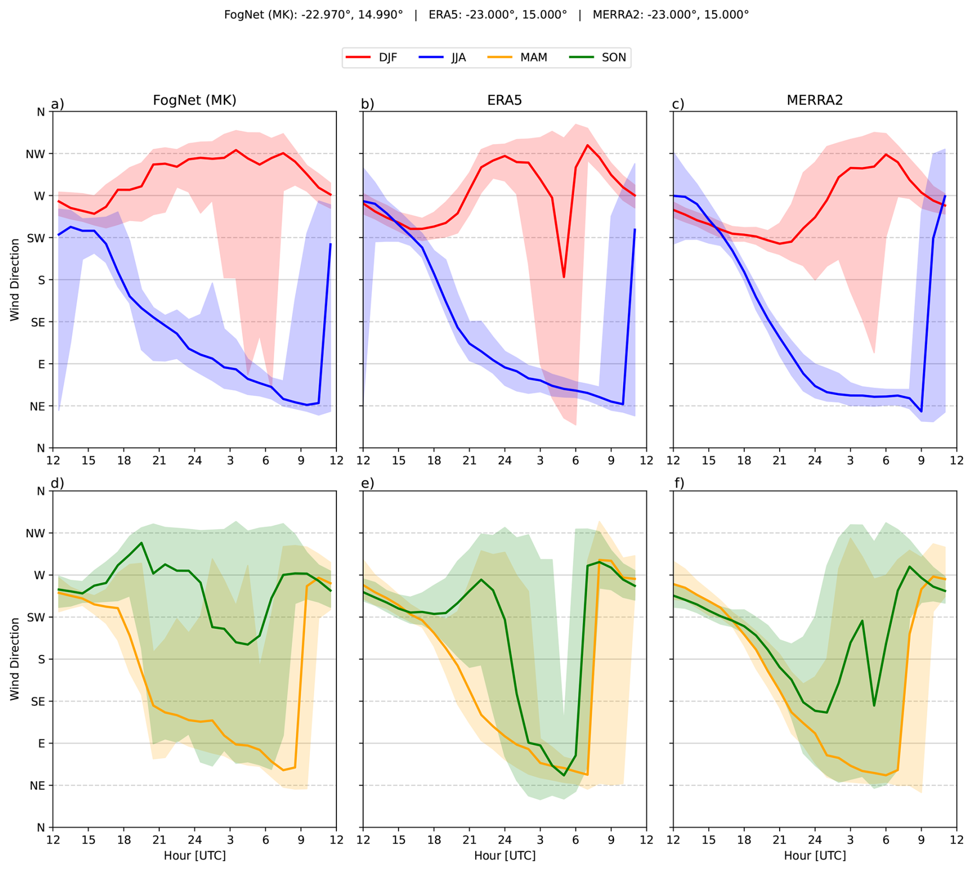
Figure B4 Seasonally averaged diurnal wind direction cycle for 2016 (red: DJF; blue: JJA; orange: MAM; green: SON). Shaded areas indicate the interquartile range (25th–75th percentile) for each hour. Top row: (a) FogNet station (Marble Koppie: 22.97° S, 14.99° E), (b) ERA5 (nearest grid cell), (c) MERRA-2 (nearest grid cell). Bottom row: (d–f) as in (a)–(c), for MAM and SON.

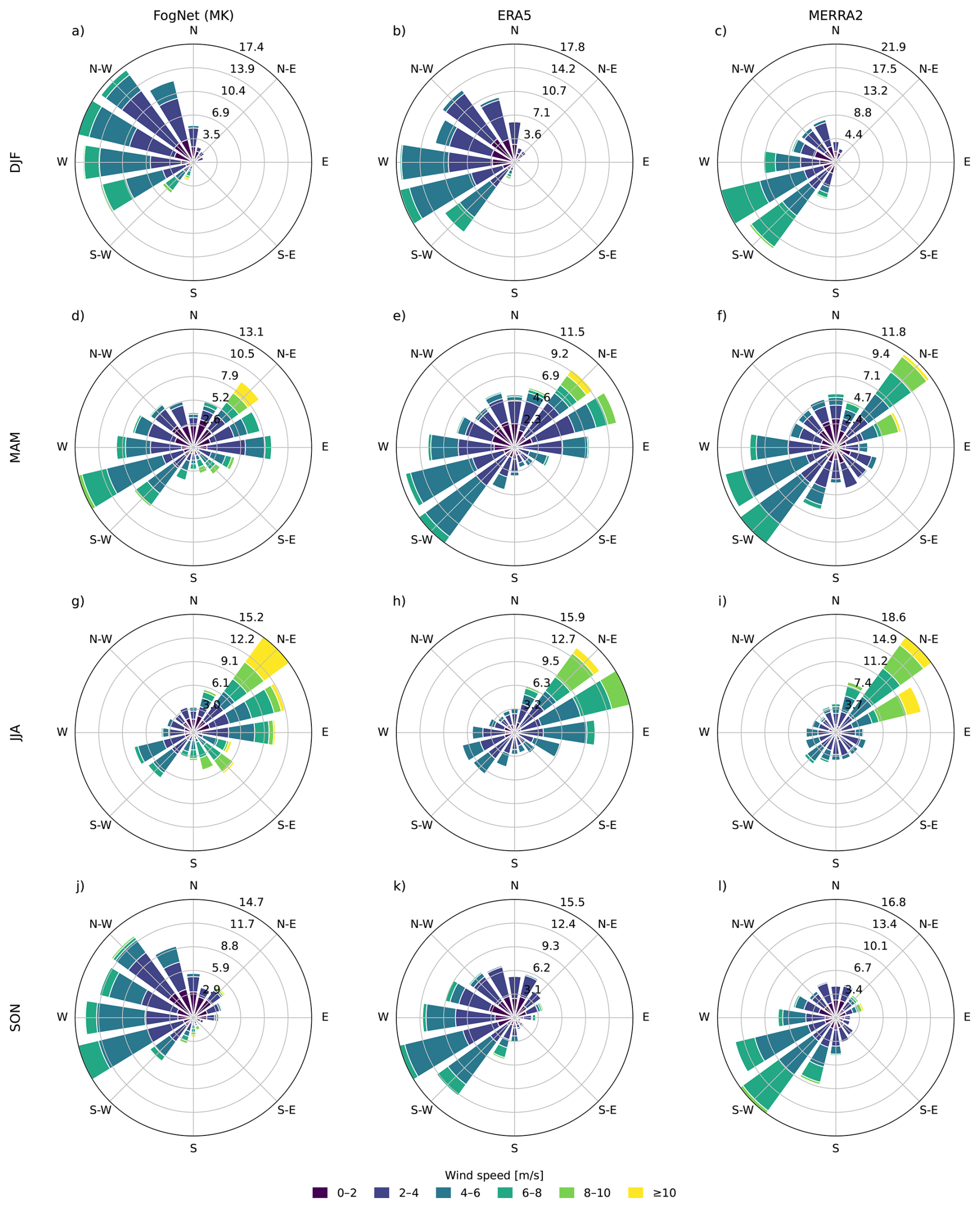
Figure B5 Wind roses showing the joint distribution of wind direction and speed for the FogNet station (Marble Koppie), ERA5, and MERRA-2, separated by season (rows: DJF, MAM, JJA, SON) for 2016. Bars indicate the frequency of occurrence (%) for each wind direction sector, colored by wind speed bin (m s⁻¹).

Appendix C: ONI/BNI/LUCI correlations for the MERRA-2 configuration

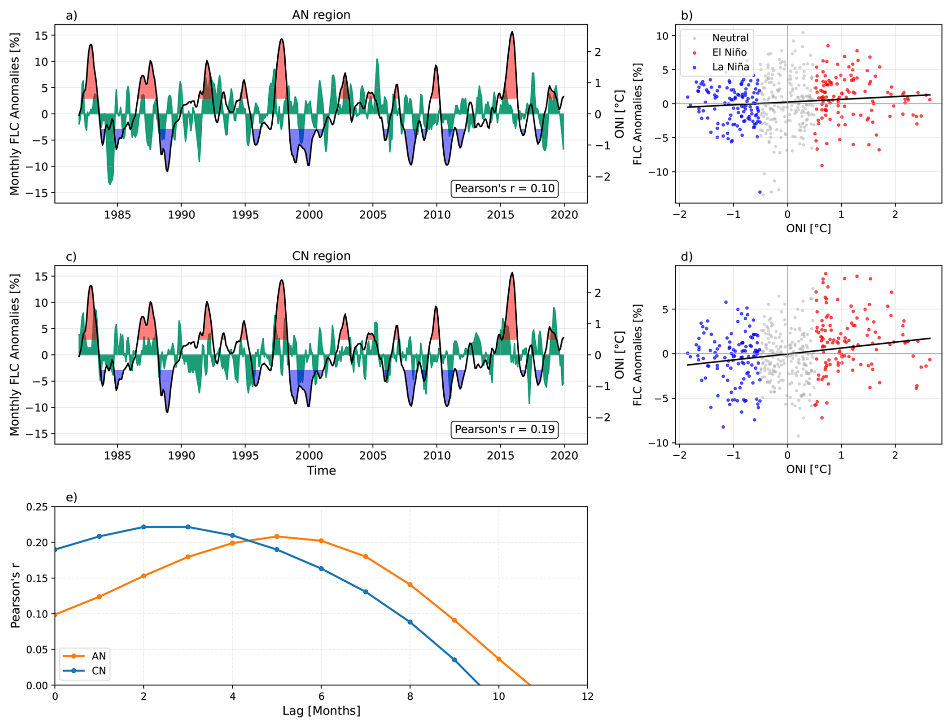
Figure C1 Detrended 3-month running mean FLC cover anomalies compared with the Oceanic Niño Index (ONI) during 1982–2019 for: AN-MERRA-2 (a) and CN-MERRA-2 (c). FLC anomalies are green and ONI black, with warm ($\ge +\mathrm{0.5}\mathrm{°}\mathrm{C}$) and cool ($\le -\mathrm{0.5}\mathrm{°}\mathrm{C}$) phases highlighted in red and blue. (b, d) Corresponding scatter plots of FLC anomalies against the ONI, with points coloured by phase (red: warm; blue: cool; grey: neutral) and the least-squares fit in black. (e) Pearson correlation coefficients (r) between lagged FLC anomalies and ONI as a function of monthly lag for AN (orange) and CN (blue).

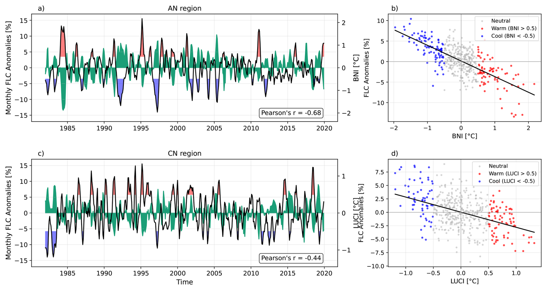
Figure C2 Detrended 3-month running mean FLC cover anomalies in the MERRA-2 setup during 1982–2019, compared with the Benguela Niño Index (BNI) for the AN region (a) and the Lüderitz Upwelling Cell Index (LUCI) for the CN region (c). FLC anomalies are shown in green, and BNI/LUCI in black, with warm ($\ge +\mathrm{0.5}\mathrm{°}\mathrm{C}$) and cool ($\le -\mathrm{0.5}\mathrm{°}\mathrm{C}$) phases highlighted in red and blue, respectively. (b, d) Corresponding scatter plots of FLC anomalies against the respective index, with points coloured by phase (red: warm; blue: cool; grey: neutral) and the least-squares fit in black.

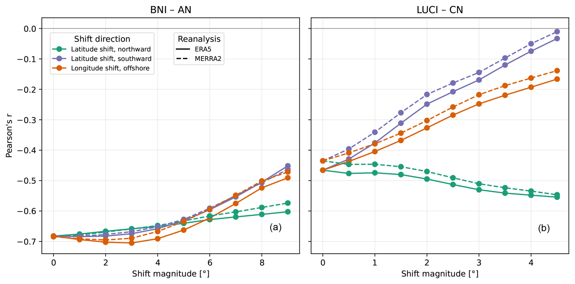
Figure C3 Sensitivity of the Pearson correlation between the BNI/LUCI indices and the reconstructed AN/CN FLC anomalies to shifts in the defining box location. The box is shifted northward, southward, and offshore (westward) from its original location (0° shift), in 1° increments for BNI and 0.5° increments for LUCI, for both the ERA5 (solid) and MERRA-2 (dashed) configurations. (a) BNI–AN. (b) LUCI–CN.