Instantaneous radiative forcings due to the first indirect effect linked to low-level liquid clouds in the Amazon

Much of the present uncertainty in effective radiative forcing due to aerosol–cloud interactions (ERFaci) arises from aerosol–cloud adjustments. Nevertheless, estimating instantaneous radiative forcing due to aerosol–cloud interactions (IRFaci) remains important because it provides observation-based benchmarks for model evaluation. Such estimates are particularly scarce for low-level liquid Amazonian clouds, particularly from approaches combining surface-based remote sensing with in situ aircraft observations. Here, we estimate IRFaci for low-level liquid clouds over Amazon using the GoAmazon2014/5 datasets. Cloud microphysical properties were constrained with ground-based remote sensing and in situ measurements, used to configure cloud representations and coupled to libRadtran simulations of daily top-of-atmosphere upward irradiance. To reduce uncertainty in baseline atmosphere, two clean reference states are defined, including one designed to represent the seasonal variability of natural background aerosol conditions. Campaign-mean IRFaci values were −11.8 W m⁻² (interquartile range: −23.0 to −2.4 W m⁻²) and −1.3 W m⁻² (−5.8 to 0.3 W m⁻²) for the two reference-state definitions. The first estimate matches the maximum literature IRFaci per AOD unit in Amazon; the second is in order of magnitude with IPCC's global mean IRFaci, −0.7 ± 0.5 W m⁻². Sensitivity tests for 2014 showed a dependence of IRFaci on aerosol load under clean conditions, decreasing with higher loads. Although it does not quantify aerosol–cloud adjustments or ERFaci, this research provides an observationally constrained estimate of IRFaci in the central Amazon, serving as a benchmark for future Amazon-focused studies of ERFaci.

1 Introduction

Anthropogenic factors generate disturbances in the global climate system and cause climatic radiative forcings (RF), defined as differences in global net irradiance between a reference atmospheric state and a state perturbed by an external climate agent (IPCC, 2013). The radiative imbalance caused by RF can prompt the atmosphere to seek a new equilibrium through variations in its internal temperature (IPCC, 2013). This re-equilibration can be modulated by the temperature of the oceans and/or continents (Levitus et al., 2012; Trenberth et al., 2014), whether or not adjustments are made to the tropospheric and/or stratospheric temperature profiles (Solomon et al., 2010; Santer et al., 2013). Effective radiative forcings (ERF) are calculated after these profiles have adjusted and reached a new radiative balance. In contrast, instantaneous radiative forcings (IRF) are obtained when no changes in temperature profiles are considered (IPCC, 2013).

Atmospheric aerosols act as cloud condensation nuclei (CCN) and ice nucleation particles (INP), playing a crucial role in cloud formation (Petters and Kreidenweis, 2007). Aerosol–cloud interactions (ACI) influence cloud microphysics (Wang et al., 2024), altering the droplet size distribution (Cecchini et al., 2016), optical properties (Zhao and Garrett, 2015), lifetime (Albrecht, 1989) and precipitation formation (Machado et al., 2018). Consequently, ACIs involving anthropogenic aerosols significantly affect global radiative balance and represent one of the main sources of uncertainty in climate models (Forster et al., 2021). The radiative forcing resulting from ACI (RFaci) can also be categorized as effective (ERFaci) or instantaneous (IRFaci). ERFaci accounts for adjustments in the initial changes in cloud droplet and ice crystal formation rates. These adjustments stem from variations in cloud fraction (f_c), cloud liquid water content (LWC), convective intensity, precipitation efficiency, and cloud lifetime, in addition to cloud formation or suppression in remote areas due to altered atmospheric circulation (Forster et al., 2021). IRFaci corresponds to the increase in cloud optical depth and albedo for a constant LWP or LWC (the equivalency between LWP and LWC occurs if the geometric thickness of the cloud does not change). Environments with high aerosol concentrations increase the number of small droplets of clouds, increasing the albedo of the cloud that reflects more radiation to space – a mechanism known as the “cloud albedo effect”, the “Twomey effect”, or the “first indirect aerosol effect” (Twomey, 1974, 1977).

The estimation of ERFaci and IRFaci on global and regional scales has been the focus of many studies (e.g. Dong and Mace, 2003; Lebsock et al., 2008; Hasekamp et al., 2019; Diamond et al., 2020). The complexity in quantifying RFaci lies mainly in representing the reference atmosphere (Haywood and Boucher, 2000; Hamilton et al., 2014), especially when the pre-industrial (PI) period is considered (Lee et al., 2016). This representation depends on a set of hypotheses and assumptions, including a degree of arbitrariness (Gryspeerdt et al., 2023) and constitutes an important source of uncertainty (Carslaw et al., 2013). Therefore, a detailed evaluation of the aerosol conditions in the reference state can reduce the uncertainties associated with the RFaci estimates (Gryspeerdt et al., 2023).

Warm clouds are regarded as the main mediators of aerosol radiative forcing through ACI (Heyn et al., 2017; Mülmenstädt and Feingold, 2018). Several studies have used modeling or satellite remote sensing data to quantify and analyze RFaci values associated with warm clouds (e.g. Quaas et al., 2009; Chen et al., 2014; Christensen et al., 2017; Toll et al., 2019), often disregarding continental areas. Among the more regionalized efforts (e.g. Keil and Haywood, 2003; Mace et al., 2006; Marsing et al., 2023; Wang et al., 2023; Herbert and Stier, 2023), only Herbert and Stier (2023) aimed to quantify IRFaci in the Amazon region, also using satellite sensor data. This shows that research on instantaneous forcings due to the Twomey effect in warm clouds over the Amazon rainforest remains limited, particularly when the estimates are derived from in situ or ground-based observations.

This study proposes a new method to estimate IRFaci caused by aerosol pollution in low-level liquid clouds in the central Amazon. The IRFaci calculations are based on ground-based and in situ measurements and are performed according to two distinct “clean” reference atmospheric states. We hypothesize that a reference state based on irradiance values that follow the natural seasonal variability of aerosols could reduce the uncertainties in IRFaci estimates. We also assess the sensitivity of low-level liquid-cloud IRFaci to different aerosol concentrations in the Amazonian atmosphere.

2 Methodology

2.1 Spatio-temporal domain

The annual cycle of aerosol number concentration in the Amazon is characterized by extreme variations, from 250 particles cm⁻³ during the wet season to values as high as 30 000 particles cm⁻³ in the dry season (Pöschl et al., 2010). This contrast makes the Amazon region a natural laboratory for studying aerosol–cloud interactions. In this study, datasets obtained during the GoAmazon2014/5 campaign (Martin et al., 2016), carried out in 2014 and 2015 in the Brazilian Amazon, were used. The experimental sites of GoAmazon2014/5 were selected based on seasonal timing and the prevailing wind direction. The sites designated as “T0” were located north of the city of Manaus, a region undisturbed by the urban pollution plume due to the prevailing northeasterly winds. The Sites “T1” and “T2” were positioned south of Manaus. The “T3” and “T3u” sites were located southwest of the city, alternately influenced by clean and polluted air masses (Martin et al., 2016) due to variations around the mean wind direction.

In this work, we used data collected from the T3 site (3.2° S, 60.6° W), which accommodated the largest number of instruments during both GoAmazon2014/5 campaign years. At T3, instruments operated by the U.S. Department of Energy (DoE) under the Atmospheric Radiation Measurement Program (ARM, https://www.arm.gov/, last access: 21 August 2026) were deployed, including the ARM Mobile Facility 1 (AMF-1) and the ARM Mobile Aerosol Observing System (MAOS; Uin et al. (2019)). Furthermore, during the two intensive operational periods (IOP1 and IOP2, from 1 February to 31 March 2014, and from 15 August to 15 October 2014, respectively) of GoAmazon2014/5, other instrumental platforms were also employed, such as the Gulfstream-159 aircraft (“G1”; Schmid et al. (2014)) and the HALO aircraft (High Altitude and Long Range Research Aircraft; Wendisch et al. (2016)). The HALO aircraft flew as part of a collaboration effort with the Brazilian-German project ACRIDICON-CHUVA (Wendisch et al., 2016).

2.2 Ground-based datasets

The atmospheric and cloud properties obtained by ground-based remote sensing included the f_c, the liquid water path (LWP), the cloud base height, and the cloud top height (CBH and CTH, respectively). All datasets were maintained and provided continuously by the ARM program. The data set f_c originated from a Value-Added Product (RADiative FLUX ANALysis VAP, Riihimaki et al. (2019)) that combined measurements from different radiometers to derive total, direct and diffuse short- and longwave downward and upward irradiances, as well as f_c for shortwave (Long et al., 2006) and longwave (Dürr and Philipona, 2004) radiation. The f_c values were retrieved at one-minute intervals and did not distinguish between different types of cloud.

The LWP values (sourced from the MicroWave Radiometer RETrievals VAP and with 1σ uncertainty, Gaustad et al. (2011)) were derived through an algorithm (Turner et al., 2007) that combines atmospheric thermodynamic state information – vertical profiles of air temperature, pressure, and relative humidity, used in independent steps of the Turner et al. (2007) method – with brightness temperature measurements at 23.8 and 31.4 GHz obtained by a surface-based microwave radiometer (MWR). The base and top heights of the observed cloud layers were derived from the Active Remote Sensing of Clouds VAP (ARSCL VAP, Kollias et al. (2007)) which combined measurements from a W-band ARM Cloud Radar (WACR, operating at 95.04 GHz) and a micropulse lidar system (MPL), with CBH and CTH values sampled every 5 s. An important observation is that the LWP data measured using the MWR could, in principle, be validated from in-situ LWC measurements made in clouds during flights over T3 (more on those LWC data in Sect. 2.3), when co-located spatially and temporally with cloud radar and lidar (WACR + MPL) measurements, used to estimate CBH and CTH. However, there were no cases of simultaneous measurements from the three instruments at both IOPs and, for this reason, we were unable to cross-validate the LWP data.

The total aerosol scattering coefficient (β_sct.), the total concentration of organic mass (“Total Organics” or “Org.”), the number concentration of cloud condensation nuclei (CCN) and the spectral aerosol optical depth (AOD) were the aerosol properties analyzed. The values of β_sct. were derived (Uin, 2024) using a pair of nephelometers measuring β_sct. as a function of relative humidity at intervals of one-min, at three wavelengths λ (700, 550 and 450 nm), and for two cuts in particle size (1 and 10 µm). The values of Total Organics were obtained using an Aerosol Chemical Speciation Monitor (ACSM), a mass spectrometer based on thermal vaporization and subsequent ionization of aerosol particles smaller than 1 µm (Watson, 2017).

The CCN number concentrations at the T3 site were measured using a cloud condensation nuclei particle counter (CCNC). This instrument measures aerosol concentrations by sampling air through a column with thermodynamically unstable supersaturated water vapor, which can condense on aerosol particles. The resulting grown particles are counted and sized by an Optical Particle Counter (OPC). Thus, CCNC quantifies the number concentration of particles activated as a function of the instrument's internal supersaturation (Uin and Enekwizu, 2024).

Spectral AOD values constituted the final aerosol-related variable used in this study. Due to the limited availability of samples, two complementary datasets were employed. The first was obtained from a sun photometer belonging to AERONET (AErosol RObotic NETwork; https://aeronet.gsfc.nasa.gov/, last access: 21 August 2026), an instrument equipped with a 25 cm collimator system mounted on a robotic base that can be programmed to point either toward the sky or directly at the Sun. This photometer measures spectral solar and sky radiances at eight wavelengths (340, 380, 440, 500, 675, 870, 1020, and 1640 nm) and uses them to calculate AOD values and other quantities (Giles et al., 2019), after correcting for molecular scattering and absorption caused by ozone and other atmospheric gases. The AERONET-derived AOD values used here correspond to the 500 nm wavelength, being measured at variable sampling rates (ranging from 1.9 to 551.3 min).

The AERONET's data set was complemented with AOD values retrieved from solar irradiance measurements acquired by a MultiFilter Rotating Shadowband Radiometer (MFRSR) operated by ARM. These irradiances serve as input for a VAP that applies the algorithms described by Harrison and Michalsky (1994), Michalsky et al. (2001), and Alexandrov et al. (2004) to derive spectral AOD values at six wavelengths (415, 500, 615, 673, 870, and 940 nm), with a sampling interval of 20 s.

2.3 In situ datasets

In situ measurements of the liquid water content in clouds, total water content (TWC), total cloud droplet concentration (N_d), cloud droplet size distribution (N(D)), and effective cloud droplet diameter (D_eff.) were performed using instruments onboard the G-1 and HALO aircraft.

Of the 35 flights conducted by the G-1 during IOP 1 and IOP 2, 29 flew over the retangular area (60.75° W, 3.3° S, 60.45° W, 3.1° S) of 0.2° × 0.3° centered at the T3 site and were used in this study. LWC and TWC measurements were carried out using the WCM-2000 instrument, a sensor composed of a scoop-shaped device equipped with several heated wires. Some of these wires are directly exposed to the airflow and cloud water droplets, while a separate reference wire is exposed only to the airflow. A power control system maintains constant voltage in one wire and constant temperature in the others. In the case of constant temperature operation, the “King-type” probe (King et al., 1978) uses the system's power values, relative airspeed, ambient temperature, individual wire dimensions, and the latent heat of water vaporization to calculate LWC and TWC each second (for calculation details, see the user manual available at https://www.scieng.com/pdf/WCM2000User.pdf, last access: 21 August 2026).

The N_d and N(D) values measured during the G-1 flights were obtained using the Fast Cloud Droplet Probe (FCDP; manual available at https://www.arm.gov/publications/tech_reports/handbooks/doe-sc-arm-tr-238.pdf, last access: 21 August 2026), an instrument that employs a focused laser beam to size hydrometeors based on the amount of scattered light during particle–beam interaction. The FCDP has a resolution of 3 µm, measures droplet diameters between 1 and 50 µm, and divides them into 20 equally spaced size bins.

The HALO aircraft conducted 14 research flights between September and October 2014, during the GoAmazon2014/5 IOP 2. The flights were designed to cover five distinct mission types, focusing on different processes involving clouds, aerosols, chemistry, and radiation (Wendisch et al., 2016). The flights were numbered chronologically as ACXX, with X ranging from 07 to 20. Among these, only two flew over clean densely forested areas to the north and northwest of Manaus (AC09 and AC18, conducted on 11 and 28 September 2014, respectively). Those flights were conducted over two regions practically unaffected by biomass burning plumes from the deforestation arc in the Amazon, characterizing the cleanest possible atmosphere among all flights performed, as indicated in Cecchini et al. (2016). Despite the low number of samples, these flights are representative of the cleanest possible atmospheric regime within the polluted season in the region, which is why they constitute the best available samples to characterize the second clean scenario used in this study. Given that the clouds measured during it were not directly affected by biomass-burning aerosols, those flights were selected to serve as a background reference.

LWC and D_eff. HALO measurements were obtained using the Cloud and Aerosol Spectrometer with Detector for Polarization (CAS-DPOL), a spectrometer that also measures the cloud droplet size distribution from 0.5 to 50 µm (Wendisch et al., 2016). Filtering of LWC and D_eff. for low-level liquid clouds was performed using flight altitude data (above sea level, ASL) from the Basic HALO Measurement and Sensor System (BAHAMAS), considering a maximum flight height of 3 km.

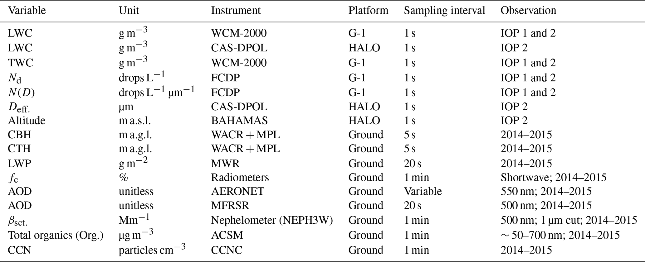
Table 1 compiles the atmospheric, cloud and aerosol variables used in this study. The table also shows the corresponding instrument, measurement unit, experimental platform, and sampling interval for each variable. For CBH, CTH, and LWP, 1 min averages were calculated to facilitate the derivation of microphysical parameters for subsequent low-level liquid-cloud modeling. For AOD, β_sct., Total Organics, CCN, and f_c, daily and/or diurnal averages were calculated. The mathematical formulations of the variables presented in Table 1 are provided in Sect. 2.4.

Table 1 Cloud and aerosol properties used in this work.

2.4 Clean and polluted scenarios

Periods with lower and higher average aerosol number concentration during the GoAmazon2014/5 campaign will be referred to as “clean” and “polluted” scenarios, respectively. The term “clean” does not imply a complete absence of anthropogenic aerosols in the atmosphere, but rather a distinctly lower concentration compared to the “polluted” scenario. The latter corresponds to episodes in 2014 and 2015 with a higher frequency of biomass-burning events and advection of the Manaus pollution plume over the T3 site.

The identification of clean and polluted scenarios during GoAmazon2014/5 was based on a visual analysis of daily means of β_sct., Org., CCN, and AOD together. Among these quantities, β_sct. and AOD are directly proportional to aerosol loading and result from the interaction between aerosols and incident electromagnetic radiation, particularly at wavelengths between approximately 0.3 and 4 µm – the solar spectrum range. This interaction is described by Mie scattering (Mie, 1908), which applies Maxwell's electromagnetic theory to describe radiation scattered by spherical particles with radius r comparable to or greater than the incident wavelength. Macroscopically, β_sct. at position s^′ along an optical path s for aerosols with refractive index n(λ) is given by Eq. (1), where N_p($r,s^{\prime }$) is the number of aerosol particles per unit air volume per size interval at position s^′, and Q_sct. is the scattering efficiency factor. Spectral AOD is related to the amount of optically active aerosols in the atmospheric column. To derive it, one must consider the solar zenith angle (θ₀, formed between the vertical direction and the propagation path of the incident radiation beam) and the linear absorption coefficient β_abs. (Eq. 2), resulting in the formulation shown in Eq. (3).

$$\begin{array}{}\text{(1)}& {\displaystyle }{\mathit{\beta }}_{\mathrm{sct}.}(\mathit{\lambda },s^{\prime })=\mathit{\pi }{r}^{\mathrm{2}}{Q}_{\mathrm{sct}.}\left[{\displaystyle \frac{\mathrm{2}\mathit{\pi }r}{\mathit{\lambda }}},n\left(\mathit{\lambda }\right)\right]\underset{\mathrm{0}}{\overset{\mathrm{\infty }}{\int }}{N}_p(r,s^{\prime })\mathrm{d}r\text{(2)}& {\displaystyle }{\mathit{\beta }}_{\mathrm{abs}.}(\mathit{\lambda },s^{\prime })=\mathit{\pi }{r}^{\mathrm{2}}{Q}_{\mathrm{abs}.}\left[{\displaystyle \frac{\mathrm{2}\mathit{\pi }r}{\mathit{\lambda }}},n\left(\mathit{\lambda }\right)\right]\underset{\mathrm{0}}{\overset{\mathrm{\infty }}{\int }}{N}_p(r,s^{\prime })\mathrm{d}r\text{(3)}& {\displaystyle }\mathrm{AOD}\left(\mathit{\lambda }\right)=\underset{\mathrm{0}}{\overset{s}{\int }}\left[{\mathit{\beta }}_{\mathrm{sct}.}(\mathit{\lambda },s)+{\mathit{\beta }}_{\mathrm{abs}.}(\mathit{\lambda },s)\right]\cos \left({\mathit{\theta }}_{\mathrm{0}}\right)\mathrm{d}s\end{array}$$

Daily means of β_sct., Org., and CCN for 2014 are displayed in Fig. 1. The period between days 10 and 90 of 2014 was selected as representative of the clean scenario, whereas the intervals between days 210–277 and 300–345 were chosen to represent polluted periods. For 2015, the same procedure was applied to the daily time series of β_sct., Org., and AOD. Figure 2, which presents these series, shows that aerosol influence peaked during the second half of the year. During the polluted period of 2015, the β_sct. and Org. peaks were greater than those observed in 2014, which exhibited a shorter clean period compared to 2015. From the time series shown in Figs. 1 and 2, the start and end days of the clean and polluted scenarios for 2014 and 2015 were determined. Table 2 summarizes these intervals and the weighted means of β_sct., Org., CCN, and AOD calculated for them. This reference will be extensively used in the calculation and analysis of IRFaci.

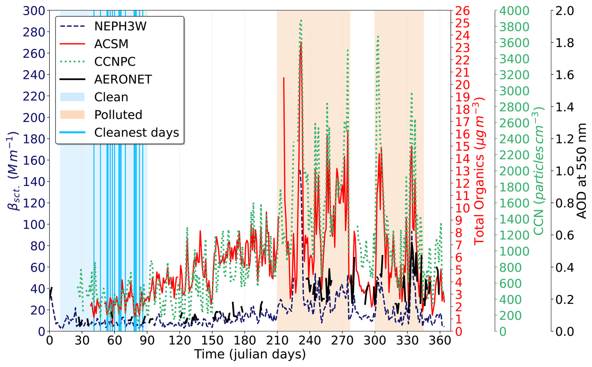
Figure 1 Daily averages of β_sct., Org. and CCN for 2014. The legend indicates the instruments responsible for data acquisition and the days that demilit the clean and polluted scenarios. The identification of cleanest days within the clean scenario was carried out using a clustering technique described in Sect. 2.4.

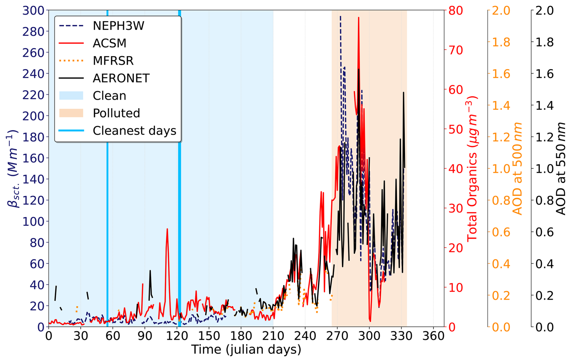
Figure 2 Daily averages of β_sct., AOD and Org. for 2015. CCN values were not considered because, for most of 2015, measurements made by CCNPC were classified as incorrect by ARM quality flags. The sparse nature of the MFRSR AOD data outside the day 150–270 window was complemented by the AERONET AOD data.

Table 2 Days that define clean and polluted scenarios for 2014 and 2015. The values in parentheses are the weighted means of β_sct., Org. and CCN (for 2014, respectively) and of β_sct., Org. and AOD from AERONET (for 2015, respectively) calculated for the corresponding interval.

The clean scenarios of 2014 and 2015 define the periods within which the cleanest days were used as the basis for the determination of the first atmospheric reference state. The selection of these cleanest days proceeded as follows: first, all days sharing common data for the variables β_sct., Org., CCN, and AOD (for AOD, since the AERONET dataset had many empty data points, only data derived from the MFRSR were considered) were identified. For these days, daytime medians (06:00–18:00 LT) were calculated for each of the four variables. After normalizing these medians, the K-Means clustering algorithm (Lloyd, 1982) was applied using 2, 3, and 4 clusters. For each cluster and each variable, a characteristic median was assigned. Comparing the medians across different cluster counts helped determine the optimal number of clusters, corresponding to cases in which no overlap occurred between the characteristic medians of distinct groups.

From the identification of optimal cluster counts for 2014 and 2015, the minimum characteristic median values were obtained, allowing the identification of the cleanest days within each clean scenario. For 2014, six days in February (11, 17, 23, 24, 26, and 28) and ten in March (2, 6, 7, 8, 12, 20, 21, 22, 25, and 28) were selected. For 2015, the cleanest days were 25 February and 3–4 May. The mean upward irradiance values at the top of the atmosphere (TOA) simulated for these days were later used as a fixed reference for the IRFaci calculations.

2.5 Extension of D_eff. and LWC measurements for the GoAmazon2014/5 period

Upward irradiance values at the TOA were calculated by the libRadtran radiative transfer code (Emde et al., 2016), which uses only LWC and r_eff. values of modeled clouds as input. Although shown here, the theoretical formulation of LWC (Eq. 4, Morrison et al. (2005), with the density of water ρ, the cloud droplet radius r, and N(D) given by Eq. 5) and of r_eff. (Eq. 6a, Stephens (1978)) were not used to calculate the LWC and r_eff.. Instead of that, the measured LWC values were used, and the r_eff. was calculated as will be explained ahead in this section. Given that in situ values of LWC, TWC, N(D), N_d, and $D_{\mathrm{eff}.}=\mathrm{2}{r}_{\mathrm{eff}.}$ were obtained only during G1 flights, the availability of these measurements was limited. Therefore, a procedure was established to increase this availability for the entire GoAmazon2014/5 period. This procedure consisted of the following:

1. Deriving empirical relationships between measured LWC and the values of r_eff., which were calculated from Eq. (6b);

2. Using surface-based datasets of CBH, CTH, and LWP to calculate LWC_ground= LWP/(CTH-CBH);

3. Inserting LWC_ground values into the empirical relationships obtained in the first step to extrapolate r_eff. for the entire GoAmazon2014/5 campaign period.

The first step to derive empirical relationships between r_eff. and in situ LWC was to consider only positive simultaneous measurements of N_d and LWC, ensuring that the aircraft was within a cloud. Subsequently, only cases with zero ice water content (IWC = TWC − LWC) were retained, thereby filtering liquid clouds. During data screening, cases where N_d<0.3 particles cm⁻³ and LWC < 0.02 g m⁻³ were excluded, removing experimental points associated with fog or extremely tenuous clouds. These filters were applied for both IOP's, with the aim of ensuring consistency of data selection for two intensive periods. Finally, r_eff. was computed according to Eq. (6b), where $<r_j>$ represents the jth mean of one of the 20 size intervals (bins) in which N(D) values were classified.

$$\begin{array}{}\text{(4)}& {\displaystyle }\mathrm{LWC}={\displaystyle \frac{\mathrm{4}\mathit{\pi }}{\mathrm{3}}}\mathit{\rho }\underset{\mathrm{0}}{\overset{\mathrm{\infty }}{\int }}{r}^{\mathrm{3}}N\left(D\right)\mathrm{d}r\text{(5)}& {\displaystyle }N\left(D\right)=N_{\mathrm{0}}{r}^m{e}^{-\mathrm{\Lambda }r}\end{array}$$

$$\begin{array}{}\text{(6a)}& {\displaystyle }{r}_{\mathrm{eff}.}={\displaystyle \frac{{\int }_{\mathrm{0}}^{\mathrm{\infty }}{r}^{\mathrm{3}}N\left(D\right)\mathrm{d}r}{{\int }_{\mathrm{0}}^{\mathrm{\infty }}{r}^{\mathrm{2}}N\left(D\right)\mathrm{d}r}}\text{(6b)}& {\displaystyle }{r}_{\mathrm{eff}.}={\displaystyle \frac{{\sum }_{j=\mathrm{1}}^{\mathrm{20}}<r_j{>}^{\mathrm{3}}N(D{)}_j\mathrm{d}r}{{\sum }_{j=\mathrm{1}}^{\mathrm{20}}<r_j{>}^{\mathrm{2}}N(D{)}_j\mathrm{d}r}}\end{array}$$

The scatterplot of calculated r_eff. versus measured LWC for IOP 1 did not show patterns that could be easily fitted by simple functions (e.g., linear or quadratic). To address this, the data were divided into 20 equally spaced LWC bins (with a width of 0.05 g m⁻³, between 0.02 and 1.02 g m⁻³), within which the LWC and r_eff. medians were calculated. The pairs of these medians were plotted and showed a particular trend, similar to that obtained by Reid et al. (1999). Like this study, those authors explored the relationship between LWC and r_eff. of liquid clouds in the Brazilian Amazon. Using in situ aircraft measurements of liquid stratiform and cumuliform clouds with bases located within the planetary boundary layer, Reid et al. (1999) concluded that after testing several fitting functions, the hyperbolic arc cosine function provided the best fit. This motivated its adoption to adjust the median pairs for IOP 1 here (Fig. 3).

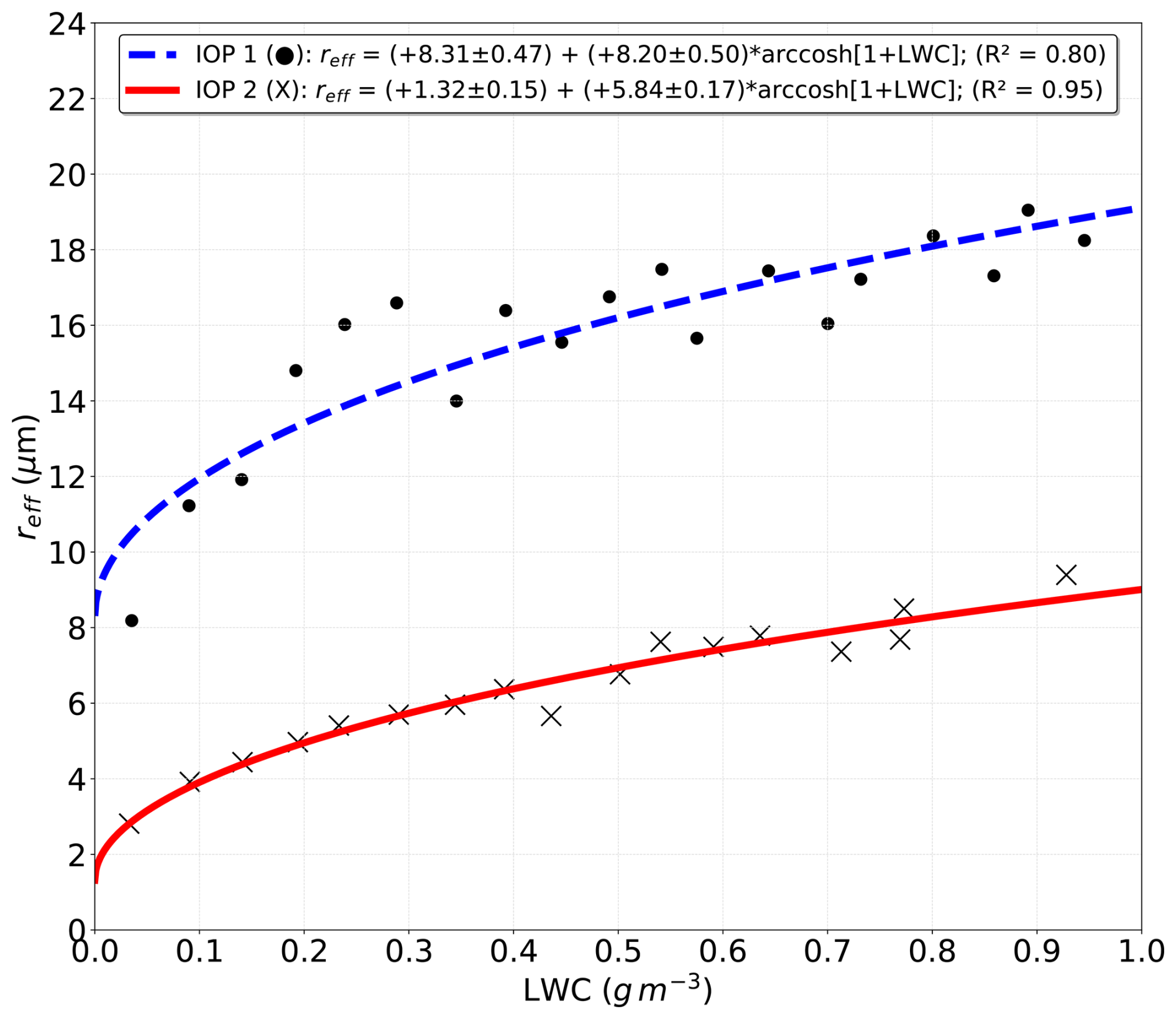
Figure 3 Dispersion of medians of r_eff. and LWC calculated in the 20 bins for IOP 1 and 2. The medians included experimental points from all altitudes where clouds with liquid water were identified and for which N_d>=0.3 particles cm⁻³ and LWC >=0.02 g m⁻³. Although no filter was applied to distinguish between cumuliform and stratiform clouds, these clouds were selected using these same filters in both IOP. The equations in the legend derived from adjustments of hyperbolic arc cosine functions to the medians shown.

For IOP 2, the scatterplot of the calculated r_eff. versus the measured LWC not showed any easily identifiable pattern also. Given that, other approach was consider LWC $/$ N_d ratios instead of N(D). In addition to this, rather than using Eq. (6b), these ratios were applied to Eqs. (7) and (8), relative to the cumulus and stratocumulus clouds, respectively (Reid et al., 1999). All the resulting values of r_eff. were considered together, without distinguishing the two types of clouds. Like in the IOP 1, the resulting data set were divided into 20 equally spaced LWC bins, and the corresponding medians were calculated. The final scatter plots for IOP 2 presented the same pattern as medians relative to IOP 1, and the hyperbolic arc cosine function provided the best fit again (Fig. 3).

$$\begin{array}{}\text{(7)}& {\displaystyle }{r}_{\mathrm{eff}.}=\mathrm{6.67}{\left({\displaystyle \frac{\mathrm{LWC}}{N_{\mathrm{d}}}}\right)}^{\mathrm{0.31}}\text{(8)}& {\displaystyle }{r}_{\mathrm{eff}.}=\mathrm{7.50}{\left({\displaystyle \frac{\mathrm{LWC}}{N_{\mathrm{d}}}}\right)}^{\mathrm{0.33}}\end{array}$$

Following the procedure to derive new r_eff. and LWC values, the second step was to use surface-derived values of CBH, CTH, and LWP to compute LWC_ground. These LWC_ground values were then inserted into the empirical relationships shown in Fig. 3, generating new r_eff. estimates for liquid clouds during IOPs 1 and 2. This procedure enabled the construction of an expanded database, covering all days within the clean and polluted periods defined by the intervals listed in Table 2, thus increasing data availability across 2014 and 2015.

For transition periods, hybrid adjustments were made using weighted averages that combined both empirical functions. For instance, during the first transition days of 2014, the calculated r_eff. values had a greater weight from the clean-period equation, while the last days were progressively influenced by the polluted-period function. This approach enabled the generation of r_eff. values as a function of LWC_ground for nearly every day of the GoAmazon2014/5 campaign, consequently allowing the modeling of liquid clouds for almost the entire observation period.

2.6 Configuration of Low-level liquid Cloud Models

The selection of low-level liquid clouds was also performed by filtering the LWC_ground and CTH datasets. The interval [0.2–0.4] g m⁻³ for LWC_ground encompasses typical values of cumulus and stratiform clouds in clean and polluted continental environments (Hess et al., 1998), and was therefore applied as a filter to the LWC_ground data. Additionally, only clouds with CTH less than or equal to 3 km were considered to ensure that the final results represented low-level clouds exclusively. Added to the filters previously applied to the r_eff. and LWC values, the filters applied to the LWC_ground and the corresponding calculated r_eff. data justify the term “low-level liquid”, which includes both shallow cumulus and low stratiform cloud types in this work.

The effective radius of liquid clouds increases with altitude in the atmosphere (Martins et al., 2011; Rosenfeld and Woodley, 2003), justifying the selection of this as a conceptual model to simulate characteristic low-level liquid clouds for each day of GoAmazon2014/5. To represent the vertical increase of r_eff. with altitude, the clouds were configured with two horizontal layers, ensuring that the r_eff. and LWC values in the models were higher in the upper layer. The base height of the modeled clouds was set according to the 12.5th percentile of CBH values, while the top height corresponded to the 87.5th percentile of the CTH data distribution. The central height was defined as the arithmetic mean between the base and top heights. The 12.5th and 87.5th percentiles of the daily r_eff. and LWC_ground distributions were similarly selected to describe the r_eff. and LWC values at the base and top, respectively, while the middle layer was represented by the median of the same distributions. Although these statistics are insufficient to explicitly capture intraday variability or transient processes, constituting a low-dimensional description, they are adequate to characterize the central tendency and dispersion of the variables mentioned. Table 3 summarizes the statistical parameters used to simulate representative low-level liquid clouds for most days of the GoAmazon2014/5 campaign.

Table 3 Configuration of “daily” modeled clouds in libRadtran, which does not require the complete droplet size distribution as input. The statistics shown were calculated from daily distributions of LWC_ground (equals the ratio between LWP and CTH-CBH difference) and of the corresponding r_eff., wich was calculated from adjusted equations shown in Fig. 3.

2.7 Radiative transfer code configuration to obtain upward irradiance at TOA

The integrated upward irradiance values (hereafter referred to as F) at the TOA were obtained using the libRadtran radiative transfer model, which applies the DISORT method (DIScrete Ordinate Radiative Transfer solver; Stamnes et al. (1988)) to solve the radiative transfer equation after accounting for adjustments to atmospheric boundary conditions. In addition, libRadtran uses the “medium” spectral resolution mode (bandwidth = 5 cm⁻¹) of the REPTRAN parameterization (Gasteiger et al., 2014) as the standard spectral configuration. The wavelength interval selected for the simulations ranged from 300 to 1000 nm, encompassing the entire visible spectrum and a small portion of the near-infrared region. The solar spectrum used extended from 250 to 10 000 nm, with a resolution of 0.1 nm.

REPTRAN is also the default method employed by libRadtran to represent atmospheric molecular scattering, applicable to both the solar and terrestrial spectra. For this, vertical profiles of the main atmospheric gases (O₂, O₃, NO₂, CO₂, and water vapor) must be provided. The “standard tropical atmosphere” file available in libRadtran already includes vertical profiles for these gases, along with profiles of air density, temperature, and pressure. The profiles of less abundant trace gases such as N₂O, CO, and CH₄ were taken from the “standard U.S. atmosphere” dataset. Considering this, the tropical atmosphere data provided by the Earth Observation Data Group (EODG) of the University of Oxford (http://eodg.atm.ox.ac.uk/RFM/atm/minor.atm, last access: 21 August 2026) were used here to generate new vertical profiles for these gases. All the profiles mentioned were used equally in all simulations, seeking to follow the definition of “instantaneous” forcing, namely, forcings obtained with the tropospheric and stratospheric profiles of constant T.

The files used to simulate representative daily low-level liquid clouds considered the exact geographic location and elevation of the T3 site. Since T3 was situated in a forested region, a surface albedo of 14 % was adopted. The mean CO₂ mixing ratios estimated for 2014 and 2015 according to the Keeling curve (Keeling et al., 2017) were also taken into account. All simulations were configured to represent upward irradiance at TOA for 16:00 UTC (12:00 LT), ensuring that the Sun was near zenith at the simulation time. Moreover, the f_c was set to 100 % for all simulations, assuming that the simulated clouds completely covered the sky at 12:00 LT. Typical examples of input files (extension .inp) used in libRadtran can be found at the link https://doi.org/10.5281/zenodo.20610494 (Pugliesi, 2026).

2.8 IRFaci estimates for the two clean atmospheric reference states

The upward integrated irradiance values at the TOA obtained from libRadtran (hereafter F_libRadtran) do not account for variations in the Earth–Sun distance (d). The necessary correction was made using Eq. (9), which assumes a plane-parallel atmosphere. The values of d and the solar zenith angle (θ₀) used in Eq. (9) were calculated using spreadsheets provided by NOAA's Earth System Research Laboratories (https://gml.noaa.gov/grad/solcalc/calcdetails.html, last access: 21 August 2026). These spreadsheets compute various astronomical parameters for any location on Earth; therefore, the d and θ₀ data were obtained specifically for the T3 site. With these parameters and the F_libRadtran outputs, the corrected irradiance values (F_corr.) were computed, accounting for temporal variations in d throughout 2014 and 2015 at T3.

$$\begin{array}{}\text{(9)}& {\displaystyle }{F}_{\mathrm{corr}.}={\displaystyle \frac{d^{\mathrm{2}}{F}_{\mathrm{libRadtran}}}{\cos \left({\mathit{\theta }}_{\mathrm{0}}\right)}}\end{array}$$

Instantaneous radiative forcings (IRF) were then calculated as the difference between F_corr. in the reference state and F_corr. in the anthropogenically perturbed state (Eq. (10)). Moreover, since the IRF calculations were based on integrated irradiances simulated for 12:00 LT at T3, the estimation of daily radiative forcing (IRF_daily, corresponding to 00:00 to 23:59 LT) required consideration of the variation of the θ₀ throughout the day. This correction was implemented using Eq. (11), which incorporated 120 values of θ₀ sampled every 6 min during daylight hours. Because T3 is located near the Equator, the durations of daytime and nighttime were considered nearly identical, and the morning and afternoon periods were approximately equal in length. For this reason, IRF_daily corresponds to either the morning or afternoon interval, justifying the division by 2 in Eq. (11).

$$\begin{array}{}\text{(10)}& {\displaystyle }\mathrm{IRF}=F_{\mathrm{corr}}^{\mathrm{reference}}-F_{\mathrm{corr}}^{\mathrm{perturbed}}\text{(11)}& {\displaystyle }{\mathrm{IRF}}_{\mathrm{daily}}={\displaystyle \frac{\mathrm{1}}{\mathrm{2}}}{\displaystyle \frac{\mathrm{IRF}{\sum }_{n=\mathrm{06}:\mathrm{00}}^{\mathrm{18}:\mathrm{00}}\cos ({\mathit{\theta }}_{\mathrm{0}}{)}_n}{\mathrm{120}}}\end{array}$$

As previously discussed, two clean atmospheric reference values were used in Eq. (10). The first, a fixed value of 689.9 W m⁻², corresponds to the mean of the corrected irradiances obtained from the cleanest days of the GoAmazon2014/5 campaign. This reference represents natural background atmospheric conditions during the 19 cleanest days of 2014 and 2015, which may differ from those characterizing the polluted periods of the same years. To account for seasonal variability in cloud microphysical properties, a second reference with variable irradiance was implemented. This approach, which consists of a first approximation to account for the natural variation in the microphysical characteristics of clouds, involved generating low-level liquid cloud models (example shown in Table 4) based on LWC data (within the [0.2–0.4] g m⁻³ interval) and r_eff. values corresponding to the cleanest conditions identified during IOP 2. The measurements used came from HALO aircraft flights AC09 and AC18, which represents the cleanest cases available among HALO flights made during the polluted period of 2014.

Table 4 Cloud configuration representing 11 September 2014 (AC09), one of the two days with measurements available during the cleanest days of IOP 2. The corresponding intervals of LWC (r_eff.) for 28 September 2014 were 0.00 to 0.24 g m⁻³ (0.00 to 5.48 µm), 0.24 to 0.27 g m⁻³ (5.48 to 8.03 µm), and 0.27 to 0.00 g m⁻³ (8.03 to 0.00 µm) for base, center, and top portions, respectively. The average LWC and r_eff. values for these two days were 0.26 g m⁻³ and 6.89 µm, respectively. The zero extremes in cloud configuration are necessary for libRadtran to correctly simulate the boundaries of the modeled clouds.

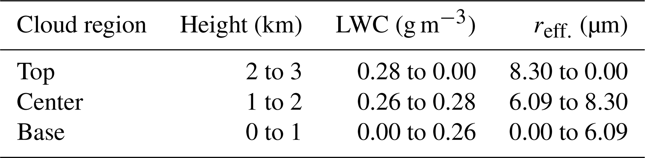
For these models, libRadtran simulated upward integrated irradiances at TOA for θ₀=0 and an Earth–Sun distance of 1 AU. The resulting irradiances, 766.7 W m⁻² and 769.1 W m⁻², yielded a mean value of 767.9 W m⁻², which was considered representative of the cleanest possible atmospheric conditions for September 2014. This mean was used as the reference for IRF calculations only during the polluted periods of 2014 and 2015. For the transitional days, reference irradiances were calculated to vary linearly (Fig. 4) between the clean and polluted reference values (689.9 W m⁻² and 767.9 W m⁻², respectively). The assumption of this linear variation between the cleanest days of the clean period and the cleanest days within the polluted period of 2014 came after an analysis of the evolution of r_eff. between these two scenarios, which occurs in an approximately linear manner throughout 2014, justifying the approximation used.

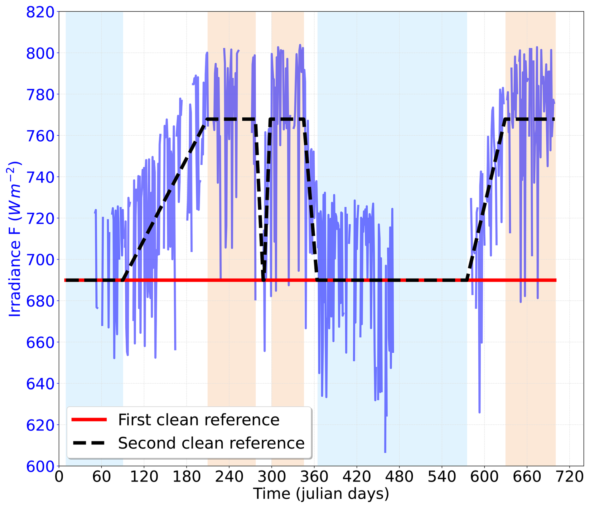
Figure 4 Integrated and corrected upward irradiances (F_corr.) at TOA for 2014 and 2015 (bluish line varying over the day of the year). The values were calculated for each day and correspond to local solar noon at the T3 site. They are also unaffected by Earth's orbital variation, so the variation over the years is due to changes in the cloud properties. The areas highlighted in blue (brown) represent the clear (polluted) periods for the two years. Days that do not show F values contain incomplete datasets (CBH, CTH, or LWP), making cloud modeling impossible. The solid (dashed) red (black) line corresponds to the F value used as a fixed (variable) reference to obtain the IRFaci estimates.

Using the seasonal reference based on aerosol availability aimed to reduce the seasonal contamination of thermodynamic variables (temperature, pressure, and water vapor profiles were the same for all simulations) and to isolate the effect of aerosols on forcings. Given that the seasonality of atmospheric dynamics affecting LWP, CBH and CTH was already embedded in the statistics of these variables, the second approach allowed the calculation of new daily forcing values less affected by the seasonal variability of natural atmospheric conditions in the T3 region.

3 Results

3.1 First clean state – “Fixed” irradiance reference

The IRF_daily values were obtained assuming a cloud fraction of 100 %. However, to regionalize the results according to the actual cloudiness observed at T3, each daily value was also multiplied by the corresponding daytime mean f_c for that specific day. Figure 5, which presents the IRF_daily values for the first clean-atmosphere reference, shows that the results incorporating the f_c measured at T3 generally display smaller absolute magnitudes compared to those associated with f_c=100 %. The observed daily oscillation arises from the way the low-level liquid-cloud models were configured – that is, based on the percentiles and medians of r_eff. and LWC. Figure 5 also clearly reveals the mean reduction in IRF_daily magnitude as the more polluted periods approach, with values becoming increasingly negative during those episodes.

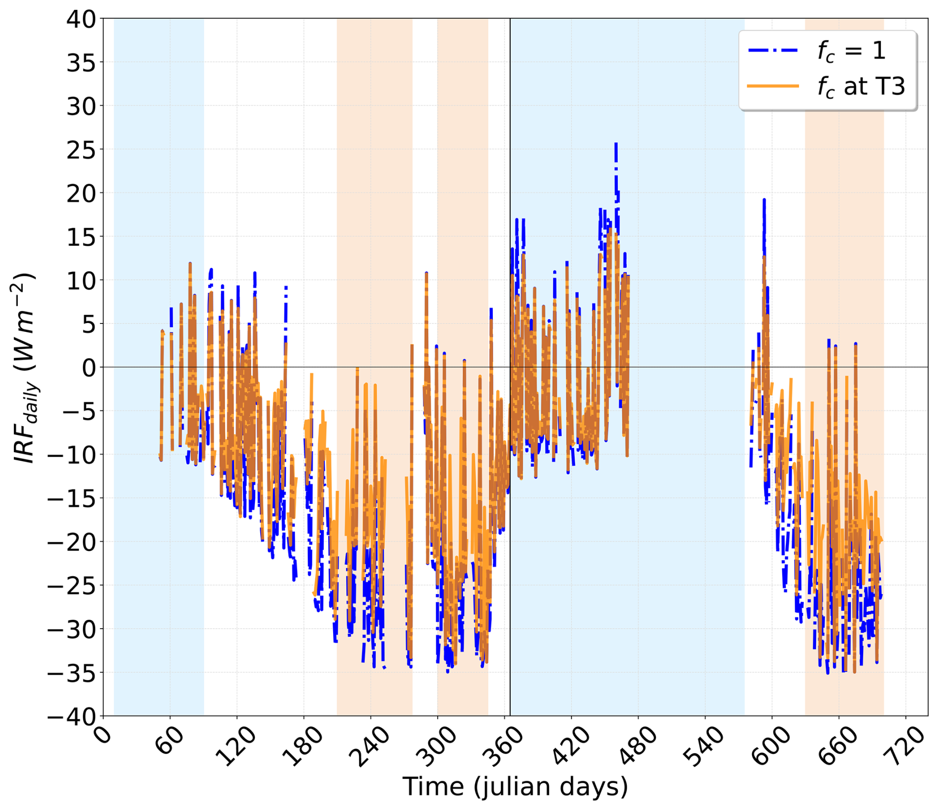
Figure 5 IRF_daily values are calculated based on the fixed clean atmosphere reference for 2014 and 2015. Blue line (f_c=100 %, the same of “f_c=1”) indicates the results for an f_c of 100 %, while the gold line shows the values according to the f_c measured at T3.

To evaluate the relative behavior of IRF_daily values across different aerosol-loading scenarios, boxplots were generated for each case. Figure 6 displays the results for 2014, along with the means and medians for each scenario. Overall, IRF_daily values that do not account for the measured f_c at T3 exhibit distributions shifted toward more negative values compared to those incorporating f_c variability, indicating that a constant f_c=100 % produces markedly stronger negative instantaneous radiative forcings. The statistics show progressively more negative values as the clean days give way to polluted ones, with results for the second 2014 transition period showing an increasing trend consistent with the decreasing aerosol parameters displayed in Fig. 1. It is also noteworthy that, although positive values occur only under the clean scenario (at the upper limit of the seventy-fifth percentile), both the means and medians for all scenarios remain negative.

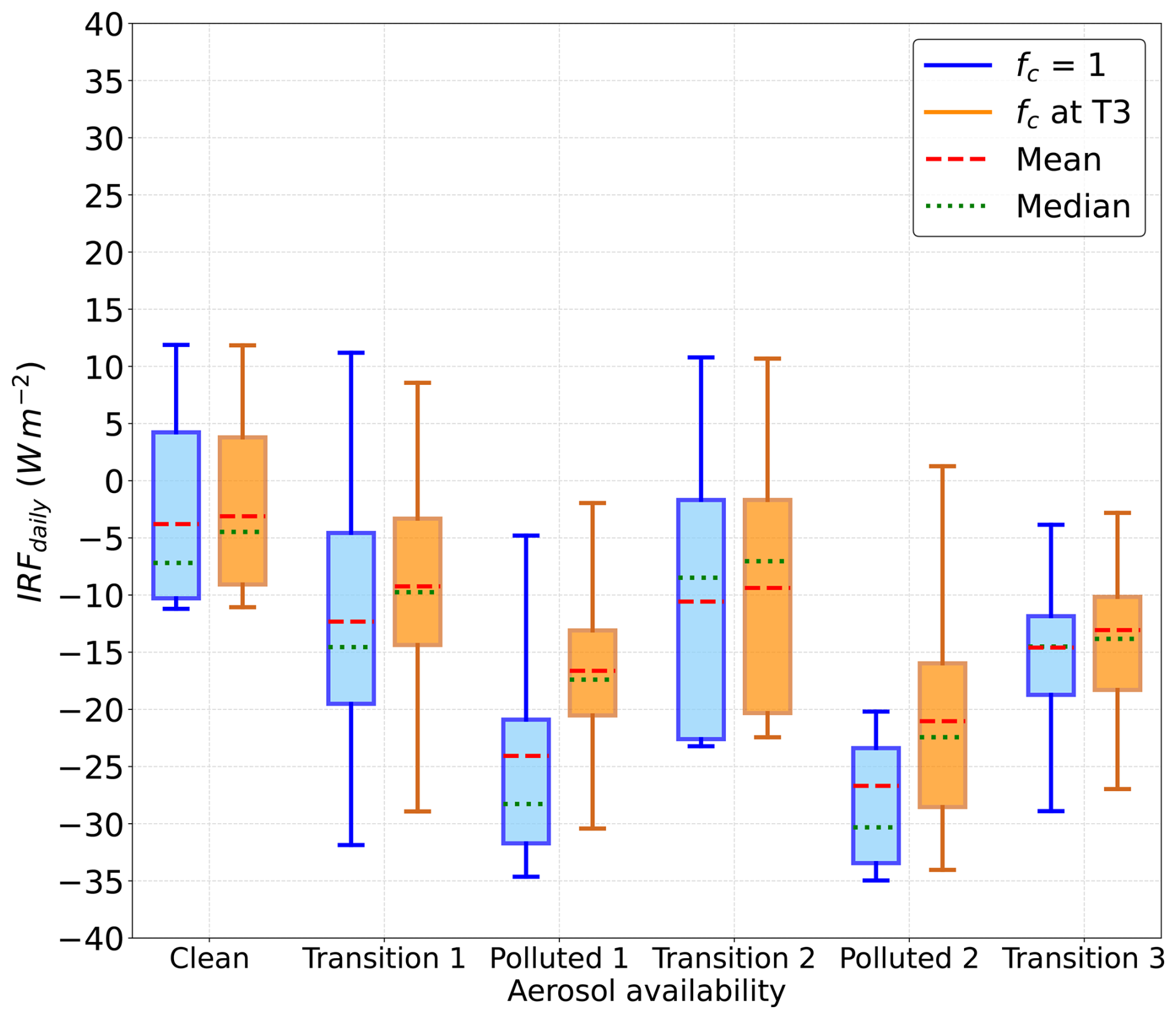
Figure 6 Boxplots, means and medians of IRF_daily calculated according to the first clean atmosphere reference for 2014 and separated according to the different aerosol availability at T3. The polluted period was divided into two subintervals due to the significant drop in concentrations of β_sct., Org. and CCN shown in Fig. 1.

The IRF_daily values computed for the polluted period of 2015 (Fig. 7) exhibit means, medians, and percentiles that are more negative than those of the clean and transitional periods of the same year. While mean and median values range from 0 to −8 W m⁻² during the clean period, the values associated with the polluted scenario lie between approximately −15 and −30 W m⁻². An important observation is that the mean IRF_daily values for f_c=100 % and for the measured cloud fraction at T3 are nearly identical under cleaner atmospheric conditions, which is not the case for the polluted scenario. This is noteworthy because – even with elevated aerosol concentrations and reduced cloud cover during polluted periods – the instantaneous radiative forcing associated with the few existing clouds is more negative than that produced by the more numerous clouds in the clean season.

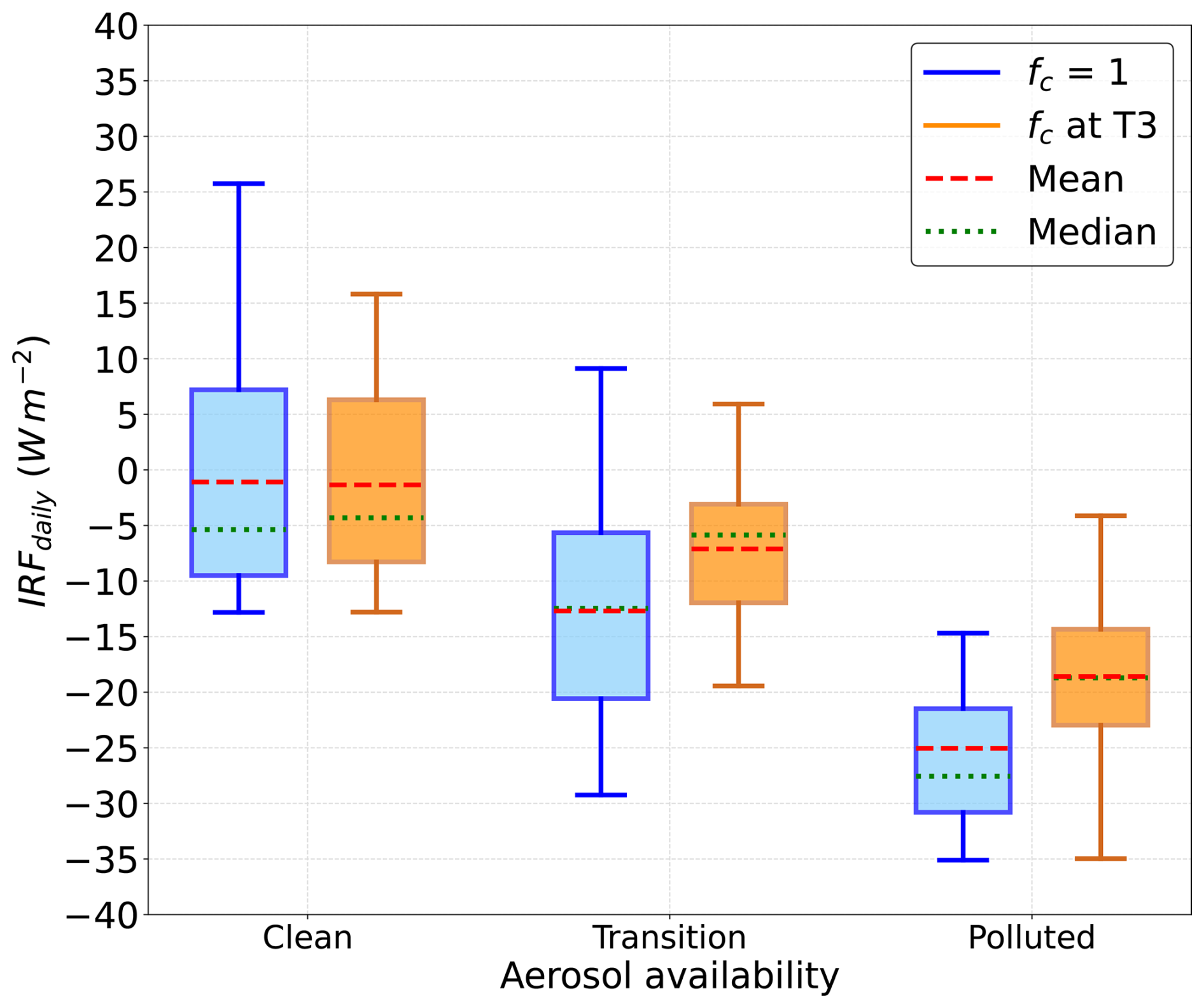
Figure 7 Boxplots, means and medians of IRF_daily calculated according to the first clean atmosphere reference for 2015 and separated according to the aerosol availability at T3.

The boxplots discussed above were complemented by histograms of the annual IRF_daily distributions for 2014 and 2015, shown in Figs. 8 and 9. The results in Fig. 8 indicate that the overall statistics for 2014 are more negative than those for 2015: the 2015 median corresponds to about 47 % of that for 2014, whereas the mean represents 66% of the 2014 mean. The results scaled by the daytime mean f_c (Fig. 9) display more homogeneous distributions approaching normality, with the lower and upper quartiles of the corresponding boxplots confined to narrower intervals than those for the distributions that ignore f_c variability at T3. This outcome suggests that multiplying by the daytime mean f_c effectively selects and constrains the final dataset, removing extreme values and producing probability density functions with reduced kurtosis magnitude.

Figure 8 Boxplots and histograms of IRF_daily for 2014 (left) and 2015 (right) for f_c=100 %.

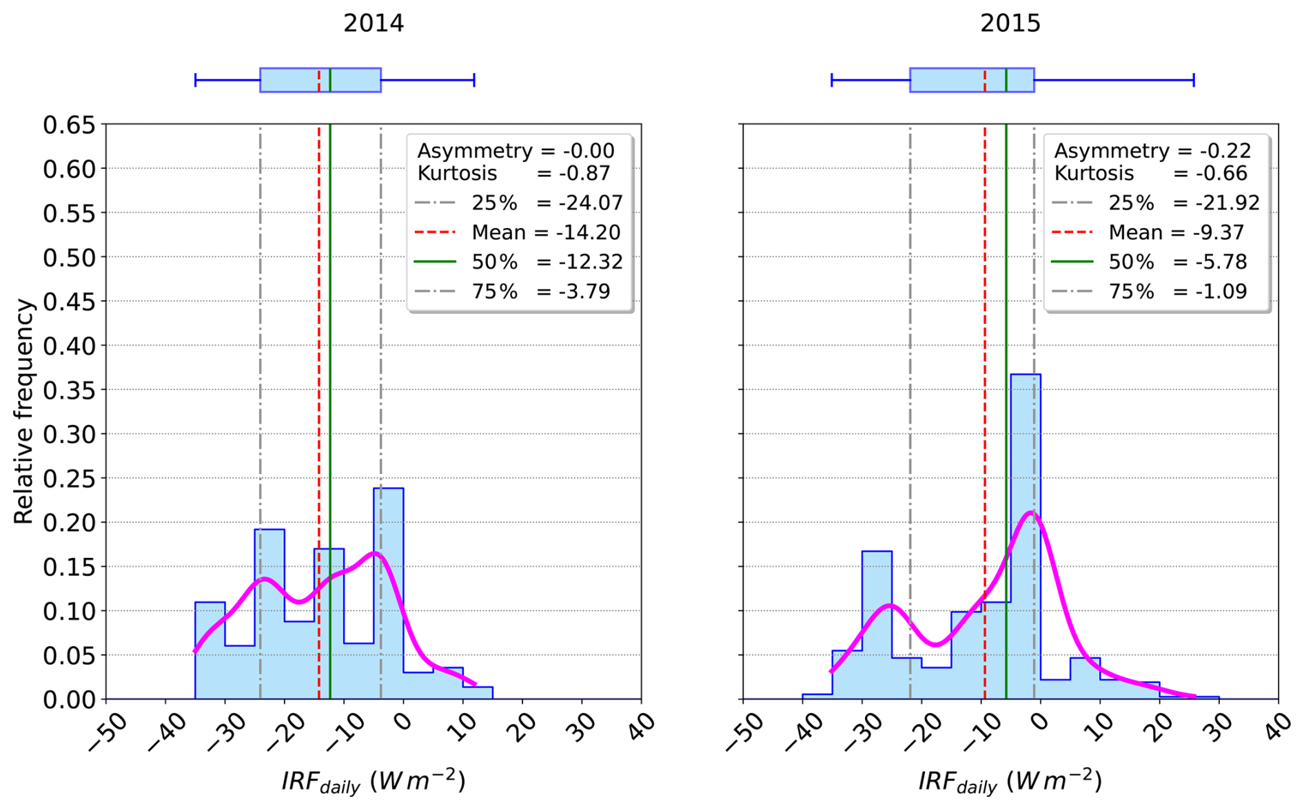
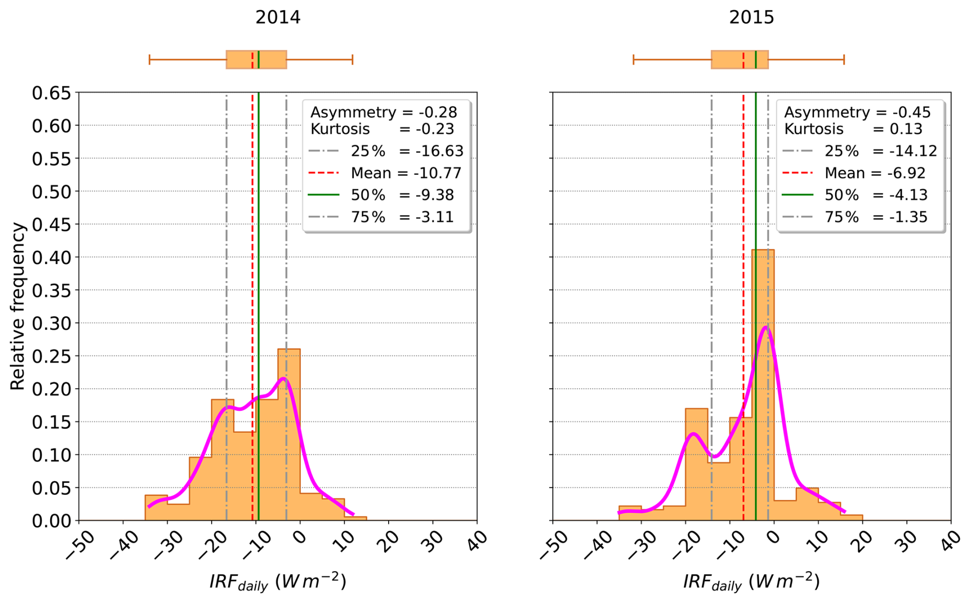
Figure 9 Boxplots and histograms of IRF_daily for 2014 and 2015 for f_c observed in the T3 site.

3.2 Second clean state – “Seasonal” irradiance reference

The IRF_daily values obtained using a variable irradiance value for a clean-atmosphere reference are presented here. It is important to recall that this seasonal irradiance reference approach aimed to reduce the likelihood that the results would be influenced by the natural atmospheric variability over T3, thus better isolating the aerosol effect on low-level liquid clouds. As shown in Fig. 10, the IRF_daily values in this case fluctuate around zero, unlike the forcings computed using the fixed irradiance reference value (Fig. 5). Nevertheless, the results are, on average, nearly constant throughout 2014 and 2015, with most data points exhibiting negative values. Subtle variations can also be observed that may or may not be associated, on average, with aerosol properties.

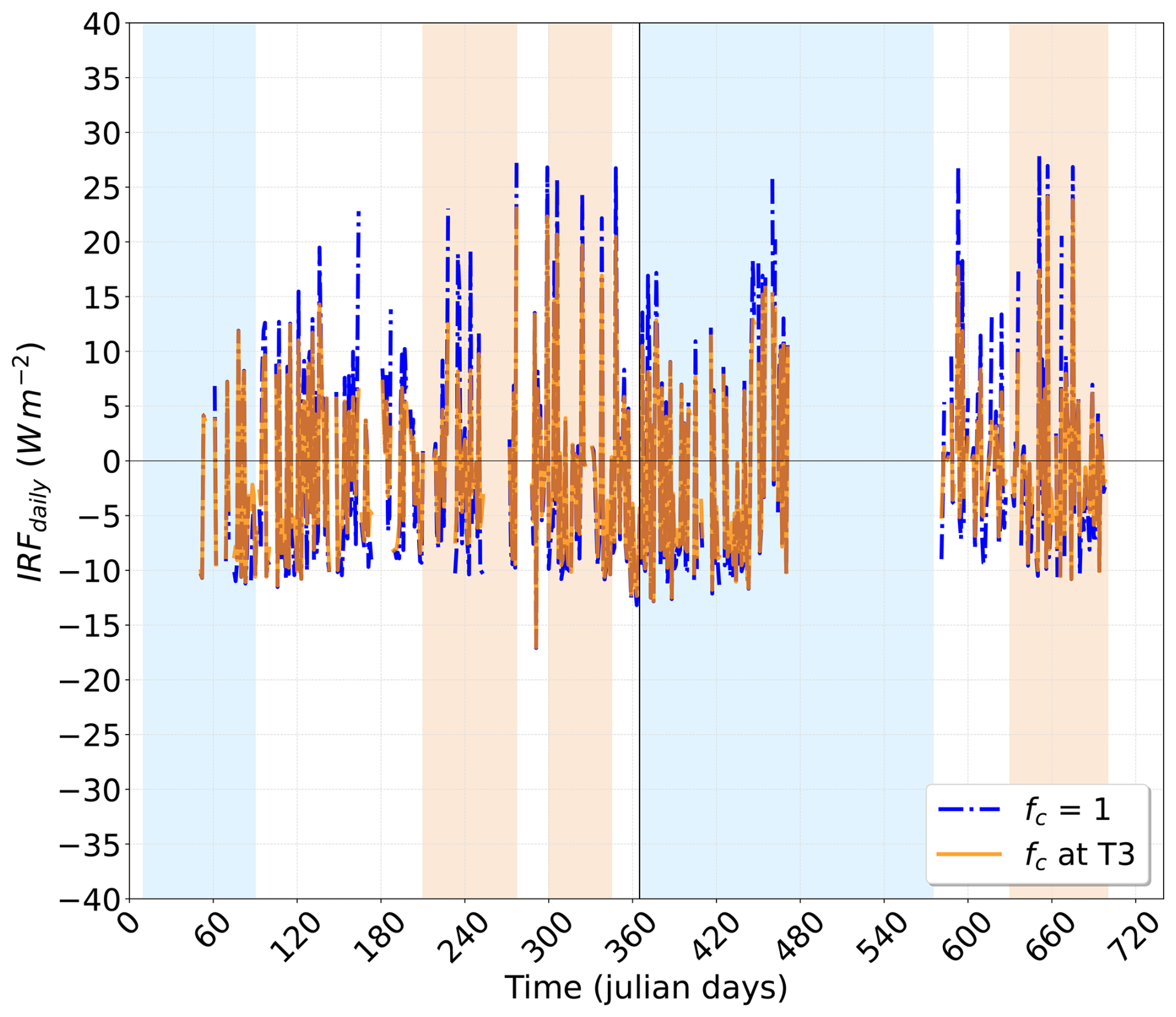
Figure 10 IRF_daily calculated according to the variable reference for clean atmosphere for 2014 and 2015. The blue line shows the results for an f_c of 100 %, while the gold line shows the values according to the f_c measured in T3. Vertical scale as in Fig. 5 for comparison.

The IRF_daily boxplots for the different aerosol-loading scenarios in 2014 and 2015 (Figs. 11 and 12, respectively) indicate that the distributions multiplied by the measured f_c at T3 are more homogeneous and less skewed than those that do not account for this parameter. The distributions for all scenarios in both years show central values (between the twenty-fifth and seventy-fifth percentiles) between −10 W m⁻² and approximately +8.0 W m⁻². The means and medians for the clean and polluted scenarios of the two years are negative, with greater magnitudes for the clean periods. This behavior, associated with a larger dispersion of IRF_daily values during cleaner conditions, can be explained – at least for the distributions that do not include the T3's cloud fraction – by greater variability in the r_eff. values of the modeled clouds in clean periods. For the results multiplied by f_c, this effect may also occur, as higher f_c values during clean conditions make the means and medians even more negative than those observed during polluted periods.

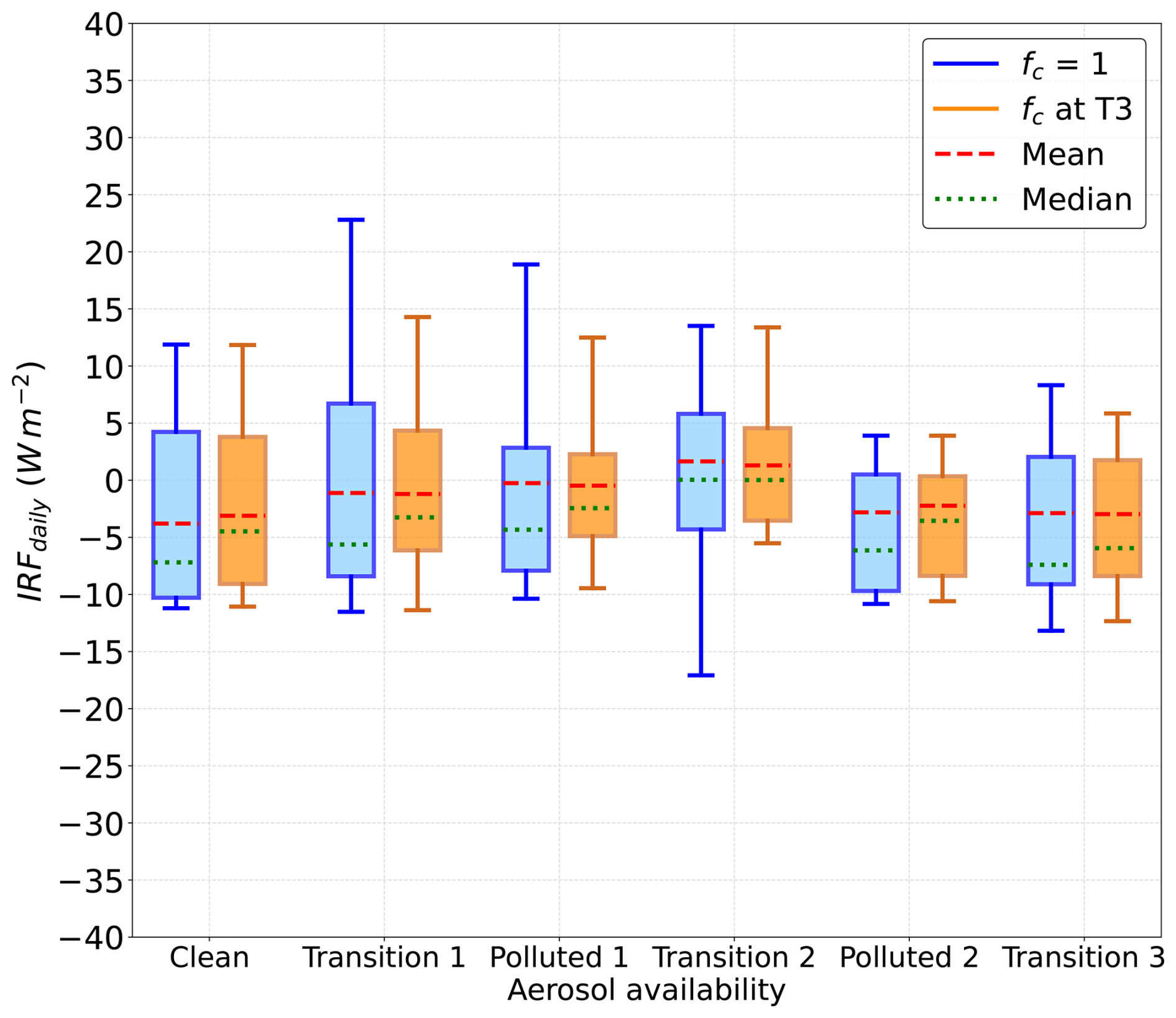
Figure 11 Boxplots, means and medians of IRF_daily calculated for the second clean atmosphere reference for 2014 and separated according to the different aerosol availability at T3.

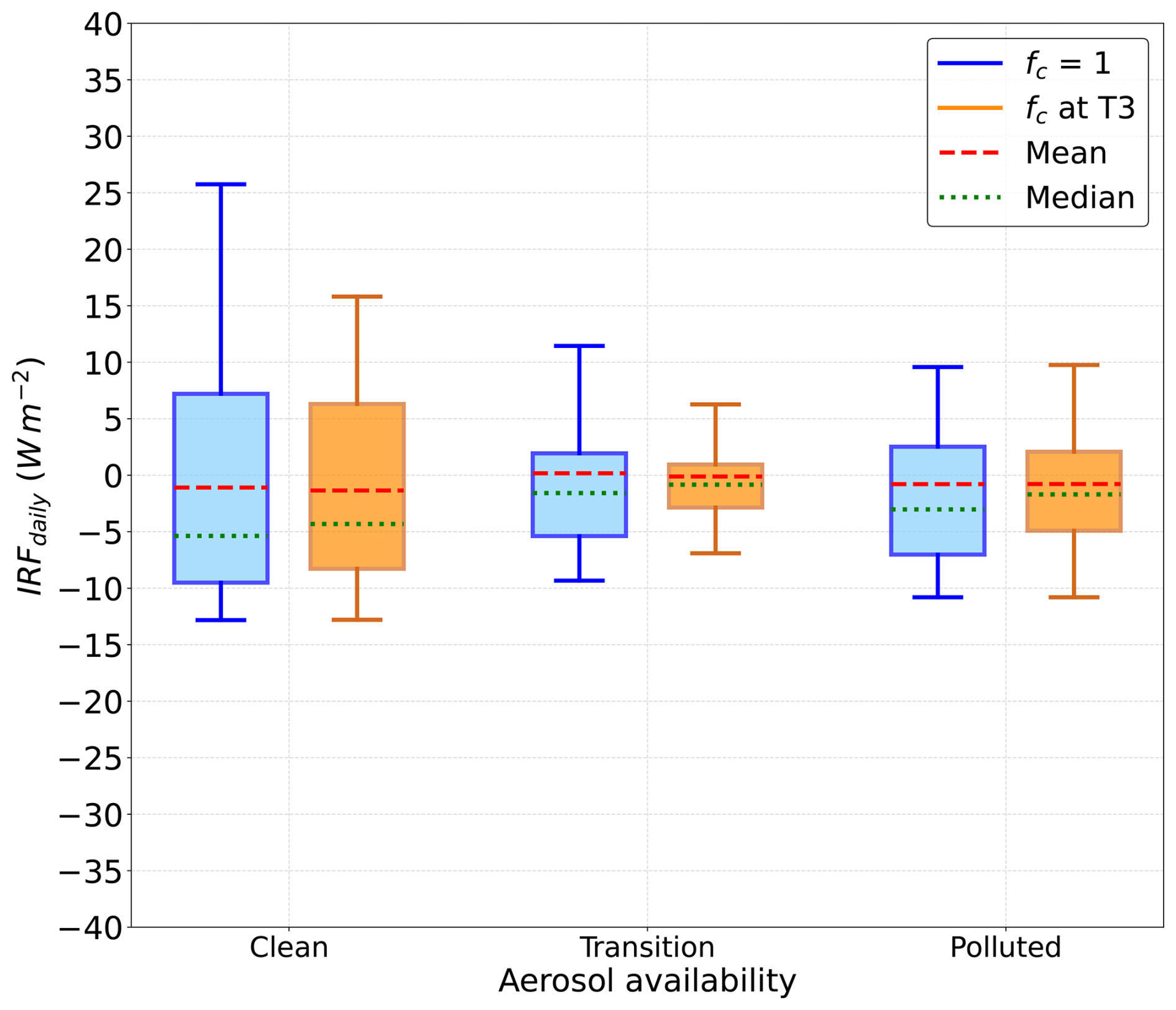
Figure 12 Statistics of IRF_daily calculated for the second clean atmosphere reference for 2015 and separated according to the different aerosol availability at T3.

The results derived from the variable irradiance reference allow the derivation of annual statistics in which the first indirect aerosol effect is more clearly isolated. The resulting statistics for 2014 and 2015 (Figs. 13 and 14) show that, compared to the values obtained using the fixed irradiance reference, the IRF_daily magnitudes are smaller. The effect of seasonal variations in atmospheric conditions on the low-level liquid cloud droplet size is illustrated by the percentage variations in the mean r_eff. during the clean periods of 2014 and 2015 relative to the mean r_eff. of the clean reference state. These differences were 21.6 % and 20.7 %, respectively, while the polluted periods exhibited reductions of 18.7 % for both years. The percentage variations in TOA flux were 1.62 % and 0.50 % for the clean intervals, while for the polluted intervals, there were increases of 0.82 % and 0.34 %, even though LWC was assumed to be the same for both clean and polluted periods.

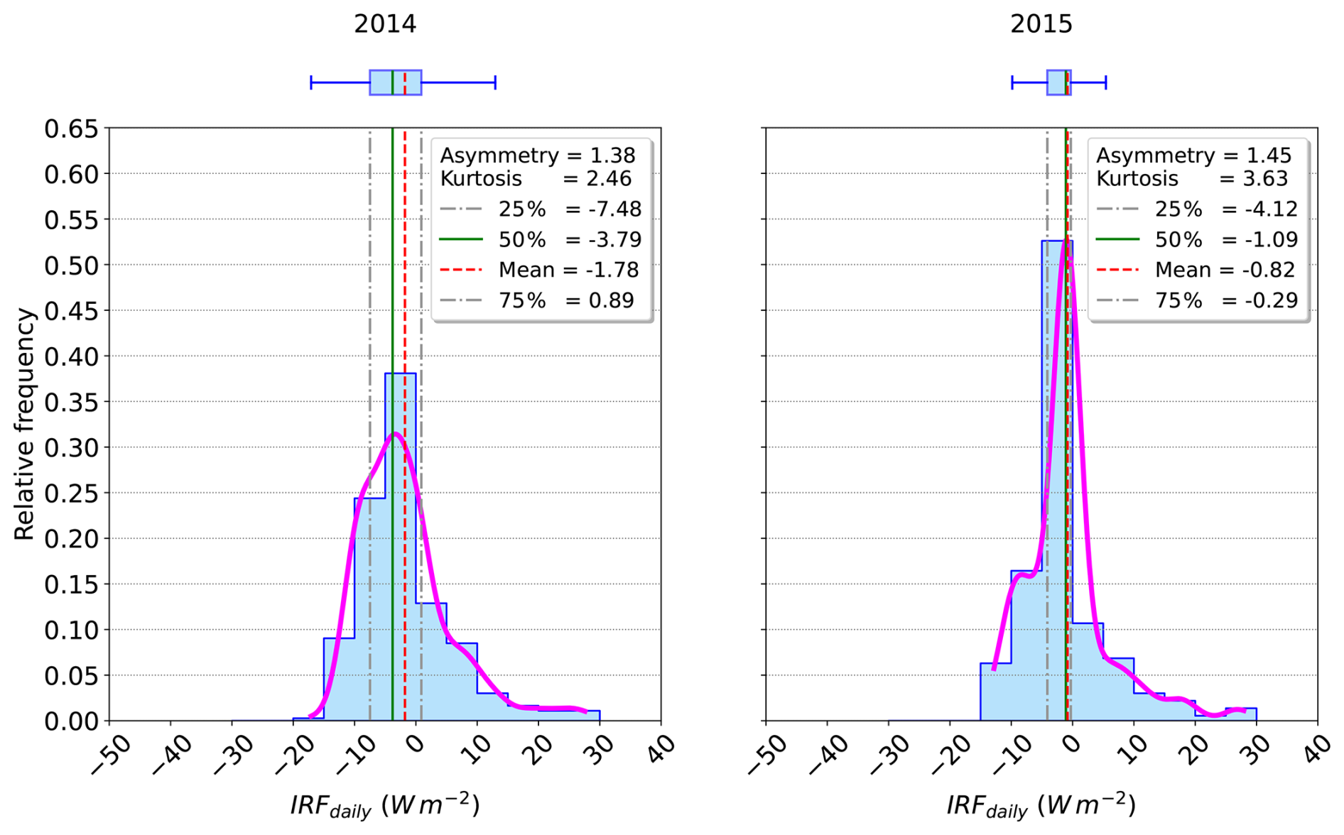
Figure 13 Boxplots and histograms of IRF_daily for 2014 and 2015 for f_c=100 % according to the second reference for a clean atmosphere.

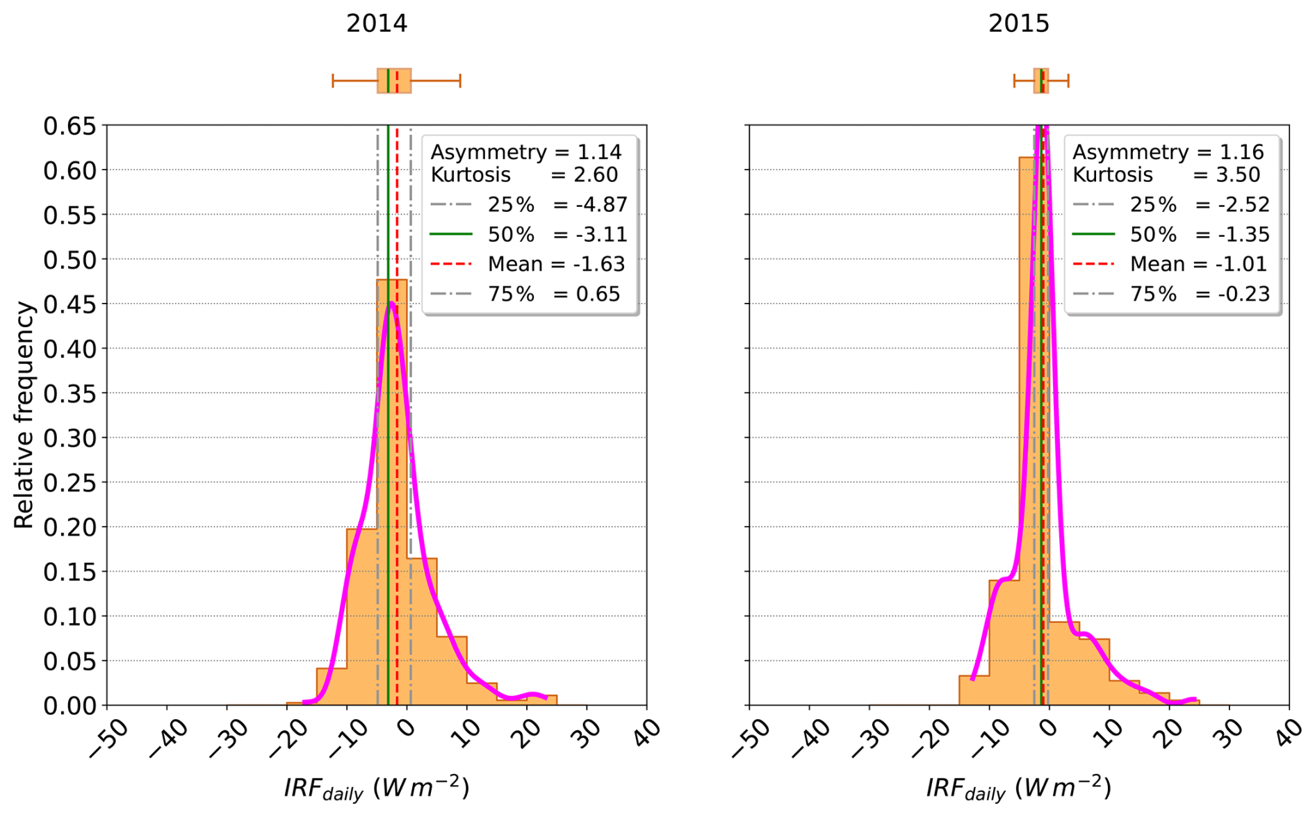
Figure 14 Boxplots and histograms of IRF_daily for 2014 and 2015 for f_c=100 % measured at T3, according to the second reference for a clean atmosphere.

3.3 IRFaci sensibilities for clean and polluted scenarios

According to Wei et al. (2020), aerosol optical depth (AOD) is widely recognized as a critical indicator to understand atmospheric physics and regional air quality due to its ability to quantify aerosol loading in the atmosphere. Considering this, one way to assess the sensitivity of daily instantaneous forcings to aerosol availability is via AOD.

In this study, the sensitivity of IRF_daily to AOD was assessed as follows: first, we calculated the daily medians of AOD for the clean and polluted scenarios of each year, and for each of these scenarios, we selected the 10 d with the lowest medians. Then, all days of a given scenario were used to calculate the average AOD (for the clean scenario of 2014, for example, we called this average “T_clean14”), while another average was calculated only for the 10 cleanest days selected previously (“t_clean14” for the clean scenario of 2014, for example). Finally, we used Eq. (12) to obtain the percentage variation of AOD within each scenario, taking “t” as the clean reference and seeking to determine by what percentage the average “T” is greater than “t”. To test the hypothesis that ΔAOD %_clean<ΔAOD %_polluted for a given year, we applied a bootstrap test and obtained the statistical significance (5 % level) of the percentage variations for each year. The results (IC = [−67.8, −23.4], p-value = 0.00 and [−16.1, 21.9], p-value = 0.92 for 2014 and 2015, respectively) show that the hypothesis was confirmed only for 2014. As with AOD, the average IRF_daily values for each scenario and for the 10 cleanest days within each scenario were calculated ($T_{{\mathrm{IRF}}_{\mathrm{polluted}\mathrm{14}}}$ and ${\mathrm{t}}_{{\mathrm{IRF}}_{\mathrm{polluted}\mathrm{14}}}$, for example). The difference between these averages ($\mathrm{\Delta }{\mathrm{IRF}}_{\mathrm{daily}}=T_{\mathrm{IRF}}-t_{\mathrm{IRF}}$) was used to calculate sensitivity S (Eq. 13, with units of $\mathrm{W}{\mathrm{m}}^{-\mathrm{2}}{\mathrm{\%}}^{-\mathrm{1}}$), for each scenario of each year. The final step consisted of performing a new statistical significance test, considering the hypothesis that S in the clean scenario is greater than in the polluted scenario. The results (p-value = 0.00 and 0.39 for 2014 and 2015, respectively) for the confidence level of 5 % showed that this occurred only in 2014.

Table 5 Percentage variations of AOD, differences of daily IRFaci, and sensitivities according to the clean and the polluted periods of 2014 and 2015.

Table 5 presents the calculated sensitivities for the clean and polluted periods of 2014 and 2015, derived from the results based on the seasonal irradiance reference while assuming f_c=100 %. The 2014 results indicate that the sensitivity of low-level liquid clouds to variations in aerosol load may be greater under cleaner atmospheric conditions than in already highly polluted environments.

$$\begin{array}{}\text{(12)}& {\displaystyle }\mathrm{\Delta }\mathrm{AOD}\mathit{\%}=\mathrm{100}\cdot {\displaystyle \frac{T-t}{t}}\text{(13)}& {\displaystyle }S={\displaystyle \frac{\left|\mathrm{\Delta }{\mathrm{IRF}}_{\mathrm{daily}}\right|}{\mathrm{\Delta }\mathrm{AOD}\mathit{\%}}}\end{array}$$

4 Summary and Discusion

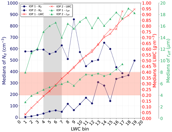
The Twomey effect related to low-level liquid clouds corresponds to the increase in cloud optical depth and albedo for a constant LWC. Those increases are caused by high aerosol concentrations that, in turn, increase the number of small droplets of clouds (the total cloud droplet concentration N_d is augmented too), becoming the dispute for water inside the cloud higher and diminishing the r_eff. of cloud droplets. This mechanism is illustrated in Fig. 15, which shows that, for a given fixed bin of LWC, the N_d and the r_eff. values vary differently for each IOP. For the [0.2–0.4] g m⁻³ LWC interval, in particular, higher N_d values and lower r_eff. values occur in IOP 2, whereas the medians of LWC remain relatively the same for both IOPs. The fact that this mechanism occurs in conjunction with the IRF_daily distribution characterized by negative medians (see Figs. 8, 9, 13, and 14) demonstrates the existence of the Twomey effect linked to the modeled low-level liquid clouds.

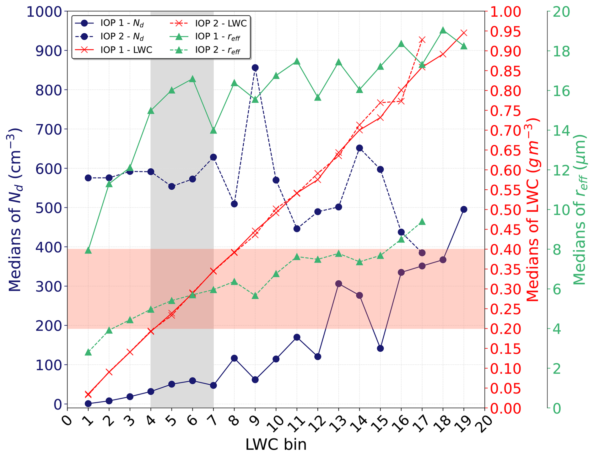
Figure 15 Medians of N_d, r_eff. and LWC according to LWC bins for both IOP. Reddish region shows the [0.2–0.4] g m⁻³ LWC interval, corresponding to bins 4, 5, 6 and 7 featured on the gray interval.

The instantaneous radiative forcings due to the first indirect aerosol effect obtained in this study were separated into those calculated using a constant irradiance reference and those derived from a seasonal irradiance reference. The annual means for f_c=100 % in 2014 and 2015, corresponding to the fixed reference, were −14.20 [−24.07; −3.79] W m⁻² and −9.37 [−21.92; −1.09] W m⁻², respectively. For the seasonal reference, the results were −1.78 [−7.48; 0.89] and −0.82 [−4.12; −0.29] W m⁻², while the interquartile ranges (IQR) were 8.37 and 3.83 W m⁻², significantly smaller than those obtained for the fixed-irradiance reference (20.28 and 20.83 W m⁻²). These results demonstrate greater IRFaci variability in 2014 than in 2015 (the interannual variability of the means was −4.83 and −0.96 W m⁻² for the first and second references, respectively) and indicate a reduced degree of uncertainty when seasonal aerosol variations are taken into account when calculating the forcings. Given that CCN and AOD concentrations were notably high during the second half of both years, these results are consistent in magnitude with previous findings (e.g. Wall et al., 2023; Wang et al., 2023).

An analysis of the probability density distributions of CBH, CTH, r_eff., LWP_ground and β_sct. for the two references showed that, despite the presence of more scattering aerosols in the second reference (medians equal to 16.8 and 4.8 M m⁻¹ for the two references, respectively) and relative discrepancies in cloud height (higher for the second reference than for the first), when compared to the most polluted days of 2014 (August and September), the second reference remains relatively clean.

For both references, positive IRF_daily values were obtained. These correspond to instances in which the reference TOA upward irradiance exceeded that of the perturbed state. This does not imply that low-level liquid clouds have a net warming effect on the surface. As cloud models were constructed from daily statistical distributions of CBH, CTH, LWC, and r_eff., the occurrence of positive instantaneous forcings arises from the adopted methodology itself, which sought to reflect the natural variability of daytime cloud properties. Furthermore, it should be noted that the days selected to represent the two reference states were chosen on the basis of aerosol availability rather than low-level liquid cloud characteristics. Therefore, daily fluctuations in irradiances and IRF_daily values are expected, representing the natural day-to-day variability of low-level liquid cloud properties.

Since the first reference, obtained using a simpler and more direct procedure, assumes a fixed irradiance value for the entire GoAmazon2014/5 period, larger IRF magnitudes are expected – particularly during polluted periods. This first reference involves fewer intermediate assumptions than the second and does not require non-contaminated data from polluted seasons. However, it neglects the seasonal variability of the atmosphere's natural conditions over the study period, which may influence the microphysics of the analyzed clouds and the resulting IRF. The variable irradiance reference, in turn, follows the seasonal atmospheric variations, reducing the likelihood that the results are biased by natural variability. Thus, although it represents a first-order approximation, the results obtained using the seasonal irradiance reference are more appropriate for analyzing instantaneous radiative forcings associated with the first indirect aerosol effect.

The differences between the IRFaci values computed using the two reference states align with Gryspeerdt et al. (2023), who emphasized the importance of clean-atmosphere states in determining resultant instantaneous forcings. The slightly higher percentage variations in integrated TOA flux during clean periods compared to polluted ones highlight the influence of cleaner atmospheric conditions on IRFaci calculations. The results in Table 5 further indicate that low-level liquid clouds may exhibit greater sensitivity to anthropogenic aerosols under cleaner conditions than in atmospheres already affected by high levels of pollution.

The daily IRFaci values obtained when considering f_c variations at T3 and using the seasonal irradiance reference were −1.63 [−4.87; 0.65] W m⁻² and −1.01 [−2.52; −0.23] W m⁻² for 2014 and 2015, respectively. The IRFaci values associated with the first indirect effect during the GoAmazon2014/5 campaign (averaged from the IRF_daily means of 2014 and 2015, for f_c= 100 %) corresponding to the two reference approaches were −11.79 [−23.0; −2.44] and −1.30 [−5.8; 0.59] W m⁻², respectively. Despite differing observational conditions (experimental platform and reference irradiance), both sets of results fall within the range reported by Herbert and Stier (2023), namely total instantaneous forcings – largely due to biomass-burning aerosols – of up to −50 W m⁻² for AOD ≈ 1.

Although direct comparison must be interpreted with caution, the second clean-atmosphere reference yielded IRFaci values in order of magnitude to the estimate (−0.7 ± 0.5 W m⁻², specifically related to the Twomey effect) reported in the latest IPCC Assessment (Forster et al., 2021). This underscores the importance of defining an appropriate atmospheric reference state in IRFaci calculations, which are significantly influenced by the chosen irradiance baseline.

5 Conclusions

Quantification of IRFaci associated with low-level liquid clouds in the central Amazon was achieved by evaluating the first indirect aerosol effect, using a unique approach that combines in situ measurements, ground-based observations, and cloud modeling based on these datasets.

The IRFaci values calculated using the fixed irradiance reference became increasingly negative as polluted scenarios approached. The averages computed for f_c=100 % and for f_c measured at T3 are virtually identical under clean atmospheric conditions, which is not the case for polluted scenarios. This indicates that, although cloud cover is greater during cleaner periods, the influence of cloud cover on the amount of radiation reflected to space becomes more significant under polluted conditions.

Using the seasonal irradiance reference reduced the variance of the resulting IRFaci, which oscillated around zero – unlike the forcings derived from the fixed irradiance reference. In addition, the IRFaci values obtained with the seasonal reference exhibited distributions with higher positive skewness, predominated by values smaller than the negative mean. The resulting interquartile range was also lower, indicating reduced uncertainties.

The results demonstrate greater IRFaci variability in 2014 than in 2015. This interannual variability depends on the aerosol load in the atmosphere, the occurrence of which varies significantly each year, depending on meteorological factors such as the occurrence of droughts or social and economic pressures, and also on public policy decisions. For the generalization of the approach used in this work to other periods, it is therefore fundamental to adequately record the daily and seasonal variations in the properties of aerosols and clouds.

The result obtained for GoAmazon2014/5 (−11.8 W m⁻² when f_c=100 % for the first clean-atmosphere reference) is an order of magnitude consistent with previous studies. The value obtained using the second reference (−1.3 W m⁻²) is of an order of magnitude consistent with the latest estimate reported by the IPCC. The percentage variations of AOD and associated IRFaci sensitivities for clean and polluted periods of 2014 (45.5 % and 81.2 %; 15.6 and 4.0 W m⁻² %⁻¹) suggest that the sensitivity of low-level liquid clouds to anthropogenic aerosols may be greater under clean conditions than in atmospheres already affected by high levels of pollution.

The results obtained stem from an effort to estimate instantaneous radiative forcings entirely from in situ and ground-based remote sensing data collected over a specific region of the Brazilian Amazon. This represents a unique approach to calculating instantaneous radiative forcings associated with the first indirect effect of anthropogenic aerosols on low-level liquid clouds in the Amazon. The findings contribute to a better understanding of the first indirect effect related to the influence that anthropogenic aerosols may exert on low liquid clouds in the central Amazon and can also serve as a reference for model evaluation and future studies aiming to quantify IRFaci or even ERFaci in that region.