Measurement report: Significant ozone loss during the Arctic winter 2020 measured from ground based microwave radiometer

Ground-based microwave observations from MIRA2 situated in Kiruna, Sweden, were used to investigate Arctic stratospheric ozone during the Arctic winter 2019/2020. A comparison of O₃ retrievals with coincident measurements of Aura MLS between 1 October 2019 and 30 April 2020 show good agreement across the investigated pressure levels (74, 56, 10, and 1 hPa). Remaining differences are well within the retrieval uncertainty of MIRA2. This demonstrates the capability of MIRA2 to provide robust ozone measurements for studies of stratospheric variability. A tracer-based approach was applied to derive cumulative chemical ozone loss on isentropic surfaces. At the 475 K isentropic (at around 50–60 hPa), ozone depletion increased from late winter into early spring, reaching a maximum loss of 2.14±0.90 ppmv in early April 2020. The magnitude and timing of the loss are consistent with the exceptional Arctic ozone depletion stated by model simulations and satellite-based estimates during the Arctic winter 2019/2020. Despite limited temporal sampling, the tracer-based method enables a consistent estimate of seasonal ozone loss from ground-based observations. The results highlight the ability of ground-based microwave radiometers to quantify chemical ozone depletion and its temporal evolution. Our results demonstrate that MIRA2 provides reliable stratospheric O₃ measurements, supporting robust monitoring of long-term ozone trends. However, our estimates of chemical O₃ depletion currently depend on MLS N₂O observations as a passive tracer. With MLS nearing the end of its mission, future chemical ozone loss assessments will require either data sets of other Earth observing satellites, expanded ground-based measurement capabilities for tracer species such as N₂O or the use of model-based tracers.

1 Introduction

Ozone is one of the most important trace gases in Earth's atmosphere, where it shields Earth's surface from the majority of the Sun's emitted ultraviolet radiation (UV). This shield, also called the ozone layer, is formed through a series of photochemical reactions first proposed in Sidney Chapman's pioneering work A Theory of Upper Atmospheric Ozone (Chapman, 1930). In this cyclic event UV splits molecular oxygen into atomic oxygen, which reacts with molecular oxygen to form ozone. Further solar UV radiation breaks up the ozone molecule to form molecular and atomic oxygen again. Chapman predicted that this process would occur between 15–35 km, to form a layer of ozone, later on commonly described as the ozone layer.

However, Farman et al. (1985) provided the first observational evidence of the Antarctic ozone hole formation during the austral spring. Building on these observations, Solomon et al. (1986) clarified the underlying heterogeneous chemical mechanisms, demonstrating that chlorine radicals can efficiently cause ozone destruction under the extreme winter and spring conditions of the polar stratosphere. Earlier, Molina and Rowland (1974) had proposed that chlorine released from anthropogenic chlorofluorocarbons (CFCs) can participate in catalytic cycles leading to stratospheric ozone depletion. This pioneering work laid the scientific foundation for international policy action, culminating in the Montreal Protocol, which mandated a global phase-out of CFC production across industrial sectors (United Nations Environment Programme, 1987).

Since the signing of the Montreal Protocol, the global reduction of ozone-depleting substances has driven significant recovery of the ozone layer, with levels moving closer to their pre-industrial state (Solomon et al., 2016; WMO, 2022). At the same time, the deployment of satellite instruments such as the Microwave Limb Sounder (MLS) aboard NASA’s Aura mission (Waters et al., 2006), along with ground-based microwave radiometers, has enhanced our ability to track ozone trends and confirm this recovery. One of these ground-based microwave radiometers is MIRA2 measuring ozone at 273 GHz, situated within the Arctic circle, at the Swedish Institute of Space Physics in Kiruna, Sweden.

Although decline in stratospheric ozone has stopped (WMO, 2022), episodes of chemical ozone depletion still occur in the polar regions under winter atmospheric conditions. A key precursor is the extremely low temperature that develops within the polar vortex during the Arctic and Antarctic winters. One of the coldest and most stable Arctic polar vortices on record occurred during the winter of 2019–2020 (Manney et al., 2022).

In this study, we present the first ozone dataset from MIRA2 collected during the winter of 2019/2020. We first assess the consistency of MIRA2 against coincident Aura MLS observations through a comprehensive cross-comparison (Sect. 5.1). Furthermore, we use MIRA2 retrievals together with coincident nitrous oxide (N₂O) measurements from MLS to quantify local cumulative chemical ozone depletion during this extraordinary winter (Sect. 5.2), placing our results in the context of previous studies (Manney et al., 2020; Wohltmann et al., 2021).

2 Previous Studies of the Northern Hemisphere Winter 2019/2020

The northern hemisphere (NH) winter of 2019/2020 exhibited one of the coldest and strongest stratospheric polar vortices on record, surpassing previously extreme winters such as 2011 (Manney et al., 2020). Persistently low planetary wave activity during December–February allowed the vortex to remain largely undisturbed (Lawrence et al., 2020), resulting in a strong and long-lived polar vortex. These conditions facilitated pronounced chemical ozone depletion, resulting in the most severe Arctic ozone loss recorded to date, as consistently demonstrated by both satellite-based observational datasets and numerical model simulations. (Manney et al., 2020; Grooß and Müller, 2021; Wohltmann et al., 2021). Strong ozone loss is often confined to the coldest air masses within the polar vortex, a low pressure system in the stratosphere that is commonly identified using potential vorticity (PV)-based diagnostics. The polar vortex size and strength can be well represented by equivalent latitude coordinates (Nash et al., 1996). The polar vortex describes a strong transport barrier at the vortex edge, which effectively limits mixing with extra-vortex air and allows the chemical evolution of isolated air masses to be tracked over time (Manney et al., 1994).

Within this isolated and persistently cold part of the vortex, conditions were favorable for widespread formation of polar stratospheric clouds (PSC). These clouds, a mixture of supercooled liquid droplets and solid particles, enable heterogeneous chemistry that activates chlorine and enhances ozone destruction. In particular, reservoir species such as HCl and ClONO₂ are converted into photo-labile forms, which upon sunlight exposure in springtime in polar regions release reactive chlorine radicals (e.g., Cl) that drive catalytic ozone loss cycles (Solomon, 1999). At the same time, denitrification caused by the sedimentation of HNO₃ containing PSC particles decreases reactive nitrogen, restricts chlorine deactivation, and thus extends the period of ozone depletion (Wohltmann et al., 2021; Manney et al., 2020).

The 2019/2020 Arctic winter polar vortex formed early, was exceptionally cold and persistent. As a consequence of these conditions, ozone depletion began unusually early, already in late November to early December, driven by low stratospheric temperature and elevated active chlorine (Wohltmann et al., 2021; Manney et al., 2020). The prolonged period of favorable chemical conditions for ozone depletion led to peak ozone loss in mid-March 2020, as indicated by simulations. By late March, ozone mixing ratios had declined to values comparable to those typically observed in the Antarctic, with total losses approaching 2.8 ppmv and near-complete depletion at the 460 K potential temperature level (Manney et al., 2020; Wohltmann et al., 2021).

3 Instruments and data

3.1 MIRA2

MIRA2 is a remote sensing microwave radiometer operated as a guest instrument at the Swedish Institute of space physics in Kiruna (67.84° N, 20.41° E, 425 m a.s.l.). MIRA2 is a heterodyne radiometer with a Schottky-diode mixer with a system noise temperature T_sys of about 1250 K (Single Side Band). The mixer is cryogenically cooled down to about 70 K by a two-stage He refrigerator. Measurements are obtained pointing North at an elevation angle between 7 and 55° depending on the tropospheric conditions. MIRA2 covers the frequency range 268 to 281 GHz, deploying an acousto-optical spectrometer with 2048 channels and a Fast-Fourier-Transform spectrometer (FFTS) with 8224 channels and 1.0 and 1.5 GHz bandwidth, respectively. With the FFTS bandwidth and 180 kHz frequency resolution a vertical profile between about 16 and 54 km can be retrieved, with a vertical resolution of about 8 km at best (Ryan et al., 2016). In the above mentioned frequency range, observation of HNO₃, N₂O, ClO and O₃ is possible. In this study, we use measurements of the ozone emission line centered at 273.05 GHz, the strongest spectral feature within the available frequency range. Although N₂O is of central importance for the ozone loss analysis described in Sect. 4.6, its emission signature in the MIRA2 spectral range is too weak to be distinguished from the measurement residuals (i.e., the instrument noise). Consequently, due to these instrumental limitations, MIRA2 has been operated exclusively in continuous ozone observation mode.

3.2 Microwave Limb Sounder

The Microwave Limb Sounder (MLS) aboard the Aura satellite is a microwave radiometer that measures a wide range of atmospheric trace gases over altitudes of approximately 5–120 km. It succeeds the MLS instrument on the Upper Atmosphere Research Satellite (UARS). Owing to extensive validation and continuous improvements in retrieval algorithms, MLS observations are widely regarded as a reliable reference dataset (Jiang et al., 2007).

The limb-sounding geometry yields a vertical resolution for ozone retrievals of about 2.5–7 km (full width at half maximum, FWHM) covering the altitude range of 5–120 km, and an effective horizontal resolution of approximately 300 km. MLS provides near-global coverage every three days. These characteristics must be considered in the analysis (see Sect. 4.3 for spatial screening and Sect. 4.4 for the application of MIRA2 averaging kernels).

In this study, we deploy Level 2 (v5.0) O₃ (Schwartz et al., 2020) products from MLS for the comparison between MIRA2 and MLS (Sect. 5.1), as well as MLS Level 2 (v5.0) ClO and N₂O (Santee, 2021; Lambert, 2021) products for the quantification of ozone loss and for the interpretation of the ozone depletion observed with MIRA2 (Sect. 5.2).

3.3 Observational data and reanalysis

Ozone measurements were collected with MIRA2 between 1 October 2019 and 30 April 2020 at the Swedish Institute of Space Physics in Kiruna, Sweden, targeting the ozone emission line centered at 273.05 GHz (Johansson et al., 2026). For the analysis and estimation of ozone loss from MIRA2 observations, it is essential to ensure that MIRA2 measurements occur within the polar vortex, which also holds for coincident measurements by MLS. In contrast to satellite measurements, ground-based measurements, such as those obtained from MIRA2, are limited to a fixed geographical location. As the polar vortex evolves in both position and shape over the course of the winter, observations at a given site may sample air passing over it, with the site located inside the vortex, within the vortex edge region, or outside the vortex altogether. This variability introduces intermittent influence from mixing processes, particularly in the vortex edge region, where ozone-rich air from lower latitudes can be advected into the measurement region (Raffalski et al., 2005).

Consequently, time series from ground-based instruments may consist of a combination of vortex and extra-vortex conditions. To ensure that measurements used for ozone loss determination represent air masses within the polar vortex, ECMWF reanalysis data (Copernicus Climate Change Service, 2019) are used to identify whether MIRA2 observations were obtained inside the vortex. Further details on the data selection are given in Sect. 4.3.

4 Analysis and methodology

4.1 Atmospheric Radiative Transfer Simulator

The Atmospheric Radiative Transfer Simulator (ARTS) is an open-source software package written primarily in C++ that enables detailed simulation of radiative transfer through planetary atmospheres. ARTS includes a comprehensive line-by-line radiative transfer model and provides tools for forward modelling as well as atmospheric retrieval applications.

In this work, ARTS (Buehler et al., 2025) and its Python interface, pyARTS (v2.6.18), are used to simulate the microwave emission spectra observed by MIRA2 and to retrieve the vertical volume mixing ratio (VMR) profile of ozone from measurements conducted during the winter 2019–2020 campaign.

4.2 Inversion model

Ozone retrievals from MIRA2 measurements are performed using an inversion model based on the Optimal Estimation Method (OEM) (Rodgers, 2000), implemented within the pyARTS framework. This statistical approach provides an optimal estimate of the atmospheric state by combining measured spectra with a priori information, each weighted with their respective uncertainties. The forward model, implemented in ARTS, describes the relationship between the atmospheric state vector and the measured radiances. The atmospheric state deployed covers approximately 0.5–78 km in altitude, with a nominal vertical resolution of about 2 km. Averaging kernel matrices and measurement response diagnostics are calculated to quantify the vertical sensitivity and to characterize the information content of the retrieved ozone profiles.

Within the OEM framework, the retrieved state vector $\widehat{\mathit{x}}$ is obtained by combining the measurement vector y with the a priori state x_a and their associated covariance matrices:

$$\begin{array}{}\text{(1)}& \widehat{\mathit{x}}={\mathit{x}}_a+{\mathbf{S}}_{\mathrm{a}}{\mathbf{K}}^T({\mathbf{KS}}_{\mathrm{a}}{\mathbf{K}}^T+{\mathbf{S}}_{\mathit{ϵ}}{)}^{-\mathrm{1}}(\mathit{y}-\mathbf{K}{\mathit{x}}_{\mathrm{a}}),\end{array}$$

where K is the Jacobian matrix describing the sensitivity of the measurements to changes in the atmospheric state, S_a is the a priori covariance matrix, and S_ϵ represents the measurement noise covariance. Measurement noise is assumed to be Gaussian and is estimated from the observed spectra.

A priori profiles for the retrieved species are primarily derived from the COSPAR International Reference Atmosphere (CIRA-86). For ozone, a climatology based on Version 8 IMK–IAA MIPAS ozone profiles, representative of the winter season for the latitude range of Kiruna, is used to provide a realistic description of the expected ozone distribution (Kiefer et al., 2023). The MIPAS O₃ profile was scaled by 75 % as this lead to stable and consistent retrievals. The a priori covariance for ozone varies with atmospheric pressure to balance the relative weighting between measurements and prior constraints. In regions with low measurement sensitivity, the retrieval is dominated by the a priori, while in regions with higher sensitivity it is primarily driven by the observed spectra.

4.3 Data selection

Coincident MIRA2 and MLS measurements were identified using combined temporal and spatial coincidence criteria. MLS overpasses of the Kiruna region occur at approximately 12:00 UTC (noon), and only MIRA2 measurements acquired within ±2 h of the overpass 12:00 UTC were considered. In addition, MLS profiles were required to lie within 400 km of Kiruna. The resulting set of coincident measurements is shown in Fig. 1 (black).

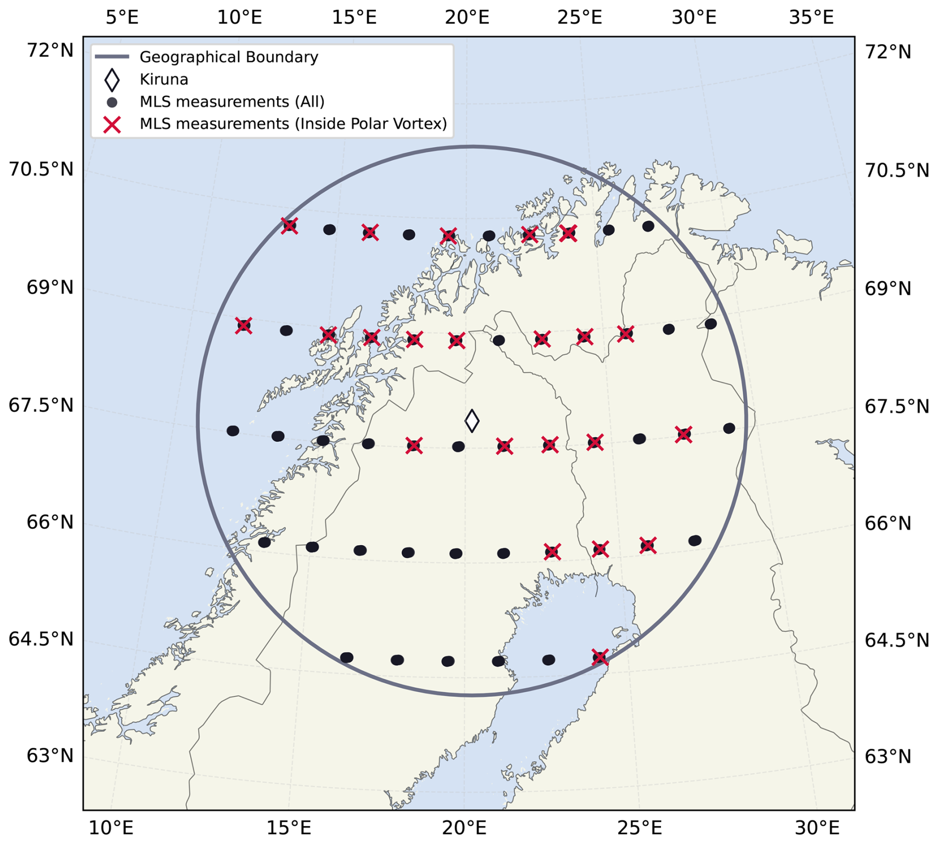
Figure 1 Coincident MIRA2 and MLS measurements from 1 October 2019 to 30 April 2020. Black markers denote MLS observations that satisfy the temporal, spatial, and quality screening criteria (456 samples). Red crosses indicate coincident inside vortex observations (145 samples). The gray circle shows the flat projection of a circle centered on Kiruna (indicated by the white diamond) with a radius of 400 km. Note that red crosses and black circles for individual days are overlaying each other and appear as single symbols.

Both datasets were subsequently filtered using retrieval quality criteria. For the MIRA2 observations, only measurements with an integration time of at least 1 h were retained to ensure a sufficient signal-to-noise ratio. Furthermore, retrievals were required to meet two conditions: (i) the residual between the fitted and observed spectra does not exceed 1 K, and (ii) the measurement response (MR) is ≥ 0.8.

The measurement response describes the fraction of information in the retrieval that is provided by the measurement rather than the a priori, and thus quantifies the sensitivity of the retrieved profile to the true atmospheric state. It is derived from the averaging kernel matrix, A, which characterizes the sensitivity of the retrieval to perturbations in the true state (Rodgers, 2000). The retrieved state $\widehat{\mathbf{x}}$ is given by

$$\begin{array}{}\text{(2)}& \widehat{\mathit{x}}={\mathit{x}}_a+\mathbf{A}(\mathit{x}-{\mathit{x}}_{\mathrm{a}}),\end{array}$$

where x denotes the true state and x_a the a priori. The measurement response at pressure level i is defined as

$$\begin{array}{}\text{(3)}& {\text{MR}}_i=\sum _j\mathbf{A}ij.\end{array}$$

Values of MR approaching unity indicate that the retrieved profiles are largely determined by the measurement rather than the a priori, whereas lower values indicate a stronger a priori influence. The applied threshold (MR ≥0.8), commonly used in atmospheric studies, ensures that at least 80 % of the retrieved information originates from the measurement (Sauvageat et al., 2022).

For calculations of the chemically induced O₃ loss, ECMWF reanalysis of potential vorticity was used to determine whether coincident MIRA2 and MLS measurements were conducted within the polar vortex. The criterion of Nash et al. (1996) was applied, and measurements satisfying this were classified as obtained inside the polar vortex (see Johansson et al. (2026)).

Moreover, for MLS data selection, recommended quality flags from the MLS Data Quality and Description (DQD) document (Livesey et al., 2022) were considered, which further constrained the dataset. To ensure that the measurements represent vortex-confined air, only observations identified as within the polar vortex in Johansson et al. (2026) were included for O₃ loss calculations (red crosses in Fig. 1). Following the application of the quality control and coincidence criteria, all accepted measurements were retained for analysis. The accepted set of measurements from MIRA2 and MLS were then averaged to produce a single representative value for each day.

4.4 MLS smoothing and re-gridding

Due to the higher vertical resolution of the O₃ retrievals from MLS (see Sect. 3.2), a direct comparison with MIRA2 profiles is not meaningful. The MIRA2 retrievals exhibit a coarser vertical resolution, approximately 10–17 km, as illustrated in Fig. 2a. To ensure a consistent comparison, the MLS altitude resolution is therefore degraded using the averaging kernels from the MIRA2 retrievals. This procedure effectively smooths the MLS profiles to the vertical sensitivity and information content of MIRA2, enabling a physically meaningful comparison between the two datasets (von Clarmann and Glatthor, 2019). The smoothing procedure is expressed in Eq. (4), where x_d denotes the degraded profile, x_a and A represent the a priori profile and averaging kernel from MIRA2, and x_h is the high-resolution MLS profile

$$\begin{array}{}\text{(4)}& {\mathit{x}}_{\mathrm{d}}={\mathit{x}}_{\mathrm{a}}+\mathbf{A}\left({\mathit{x}}_h-{\mathit{x}}_{\mathrm{a}}\right).\end{array}$$

For each comparison, the averaging kernel is selected by minimizing the temporal mismatch between coincident MLS and MIRA2 observations. Since the two datasets are defined on different pressure grids with different vertical sampling, the MLS profiles are first linearly interpolated in log-pressure space onto the MIRA2 retrieval grid, ensuring consistency between x_a, A, and x_h (von Clarmann and Glatthor, 2019). The effect of the interpolation and smoothing on the MLS profiles is illustrated in Fig. 2a, which shows the retrieved MIRA2 profile (black) alongside the original (blue) and smoothed (red) MLS profiles from a coincident measurement on 6 April 2020.

Figure 2 O₃ profiles from MIRA2 (Johansson et al., 2026) (black), original MLS (Schwartz et al., 2020) (blue), and smoothed MLS (red) with ±σ uncertainty (shaded) are shown in panel (a). Panel (b) shows the vertical resolution (black) and averaging kernel offset (red). Panel (c) shows the averaging kernels with colors associated to nominal altitude and measurement response (red). All data are from coincident MIRA2 and MLS measurements of 6 April 2020 with shaded regions indicating altitudes with MR ≥0.8.

The vertical resolution, shown in Fig. 2b (black), is determined from the full width at half maximum (FWHM) of the averaging kernel rows (Rodgers, 2000), seen in Fig. 2c. The vertical representativeness of the retrieval is further characterized by the kernel offset (Fig. 2b, red), which quantifies the displacement between the nominal retrieval pressure level and the effective altitude from which measurement information predominantly originates. Small offsets indicate that the retrieved state is representative of the specified pressure level, whereas larger offsets imply substantial contributions from adjacent atmospheric layers. Where the measurement response (MR) exceeds 0.8 (Sauvageat et al., 2022), the offset is generally small, indicating that the retrieval is primarily constrained by the measurements and that the information is associated with approximately the correct pressure level. At lower MR values, the offset increases, reflecting a greater influence of the a priori constraints and a reduced vertical fidelity of the retrieval.

4.5 Vertical coordinate for analysis

The cross-comparison and analysis of the retrieved profiles from MIRA2 are performed on the native retrieval grid (i.e. in pressure coordinates) in order to avoid interpolation artifacts and to ensure consistency with the original measurement sensitivity. Retaining the native grid is particularly advantageous for intercomparisons, as it preserves the vertical resolution and averaging kernel characteristics of the retrieval.

In contrast the ozone loss estimation is performed on isentropic surfaces of potential temperature, θ, as has been done in previous studies of Arctic winter 2020 ozone depletion (Manney et al., 2020; Grooß and Müller, 2021). We adopt isentropic surfaces of θ because they allow repeated measurements to be compared while minimizing the influence of diabatic processes (Baumgartner et al., 2020). By definition, the potential temperature accounts for the surrounding atmospheric temperature, as shown for dry air in Eq. (5), where T is the atmospheric temperature, p₀ and p are the reference ground-level pressure and the local atmospheric pressure, respectively, R is the specific gas constant of dry air, and c_p is the specific heat capacity of dry air

$$\begin{array}{}\text{(5)}& \mathit{\theta }=T{\left({\displaystyle \frac{p_{\mathrm{0}}}{p}}\right)}^{R/c_p}.\end{array}$$

This implies that observed changes in an air parcel along an isentropic surface are primarily due to adiabatic motion. Consequently, temporal changes observed at a constant isentropic surface more reliably reflect dynamical and chemical processes. This distinction is particularly important when estimating chemical ozone losses, as it allows us to separate changes in O₃ caused by vertical transport from those due to chemical reactions. Furthermore, the use of potential temperature as a vertical coordinate aligns our methodology with prior studies of the Arctic winter 2020, mentioned earlier in this section, facilitating direct comparison of results.

While potential temperature, θ, is provided for all MLS data products via the Derived Meteorological Products (DMP) dataset, in which the meteorological fields are derived from MERRA-2 (Millan et al., 2026). However, for MIRA2 observations the potential temperature is calculated using Eq. (5). For this calculation, we employ the same temperature and pressure profiles from ECMWF that are used in the retrieval process, as described in Sect. 4.2. Subsequently, all MLS and MIRA2 data are interpolated onto a common potential temperature grid, enabling direct comparison between the datasets and facilitating ozone loss calculations on fixed isentropic surfaces.

4.6 Chemical ozone loss from tracer–tracer correlations

Chemical ozone loss was quantified using the tracer–tracer correlation method (Tilmes et al., 2006), which exploits the compact relationship between ozone (O₃) and the long-lived tracer nitrous oxide (N₂O) in the winter stratosphere. Because N₂O is largely unaffected by chemical processes on seasonal timescales, its variability is primarily governed by transport and mixing. As a result, N₂O can be used as a proxy for dynamical variability in O₃. By establishing a reference relationship between O₃ and N₂O under conditions largely unaffected by chemical ozone depletion, the expected ozone abundance in the absence of chemical ozone loss, commonly referred to as passive ozone, can be estimated from observed N₂O.

The reference O₃–N₂O relationship was derived from coincident MIRA2 O₃ and MLS N₂O observations between 400 and 600 K potential temperature on 9 December 2019. This date was selected because it precedes the period of substantial chemical ozone depletion investigated in this study, thus representing the dynamical state of the early winter stratosphere. Figure 3 shows the observations used to derive the reference relationship. A fourth-degree polynomial with coefficients, a_i, was fitted to the data using orthogonal distance regression (ODR),

$$\begin{array}{}\text{(6)}& f\left(x\right)=\sum _{i=\mathrm{0}}^{\mathrm{4}}{a}_i{x}^i,\end{array}$$

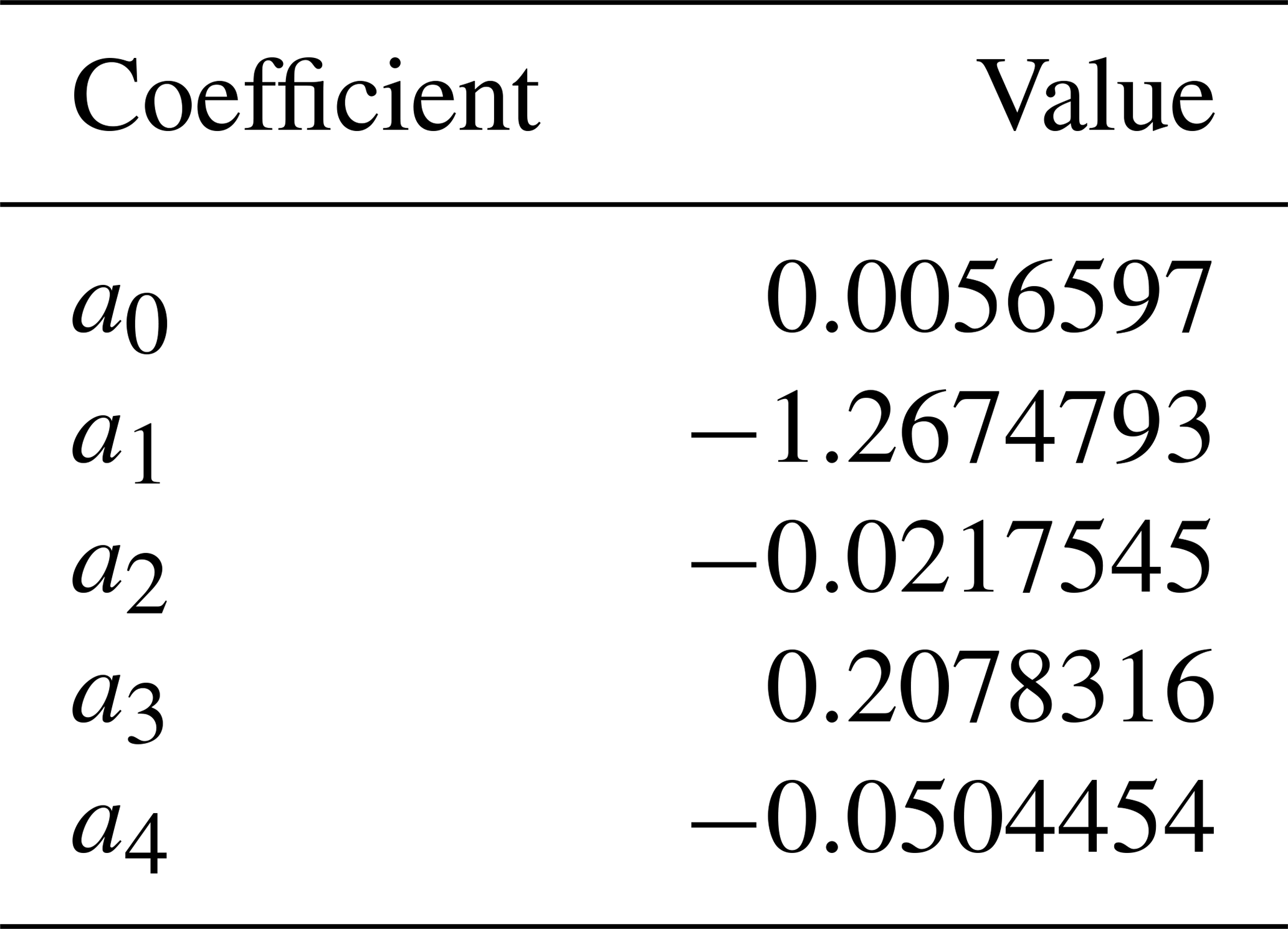
where x denotes MLS N₂O observations and f(x) represents the corresponding passive ozone abundance. ODR was chosen because it accounts for measurement uncertainties in both variables. To improve numerical stability during parameter estimation, both MLS N₂O observations (x) and MIRA2 O₃ observations (y), as well as their associated uncertainties (σ_x and σ_y), were normalized using the sample mean ($\stackrel{\mathrm{‾}}{x}$ and $\stackrel{\mathrm{‾}}{y}$) and standard deviation (s_x and s_y) which is provided in Appendix B (Table B),

$$\begin{array}{}\text{(7)}& {\displaystyle }{x}_n& {\displaystyle }={\displaystyle \frac{x-\stackrel{\mathrm{‾}}{x}}{s_x}},\text{(8)}& {\displaystyle }{y}_n& {\displaystyle }={\displaystyle \frac{y-\stackrel{\mathrm{‾}}{y}}{s_y}},\text{(9)}& {\displaystyle }{\mathit{\sigma }}_{x_n}& {\displaystyle }={\displaystyle \frac{{\mathit{\sigma }}_x}{s_x}},\text{(10)}& {\displaystyle }{\mathit{\sigma }}_{y_n}& {\displaystyle }={\displaystyle \frac{{\mathit{\sigma }}_y}{s_y}},\end{array}$$

The fitted polynomial, with coefficients a_i given in Appendix B (Table B1), describes the passive ozone VMR, O_3P, as a function of the N₂O VMR. Passive ozone was therefore obtained by evaluating Eq. (6) at the observed MLS N₂O values. Chemical ozone loss was then calculated as the difference between the measured ozone abundance, O_3M, and the passive ozone estimate,

$$\begin{array}{}\text{(11)}& \mathrm{\Delta }{\mathrm{O}}_{\mathrm{3}}={\mathrm{O}}_{\mathrm{3}\mathrm{M}}-{\mathrm{O}}_{\mathrm{3}\mathrm{P}},\end{array}$$

where O_3M denotes MIRA2 O₃ observations and O_3P denotes the corresponding passive ozone abundance inferred from the reference O₃–N₂O relationship. Deviations from the reference relationship are therefore interpreted as chemically induced ozone loss.

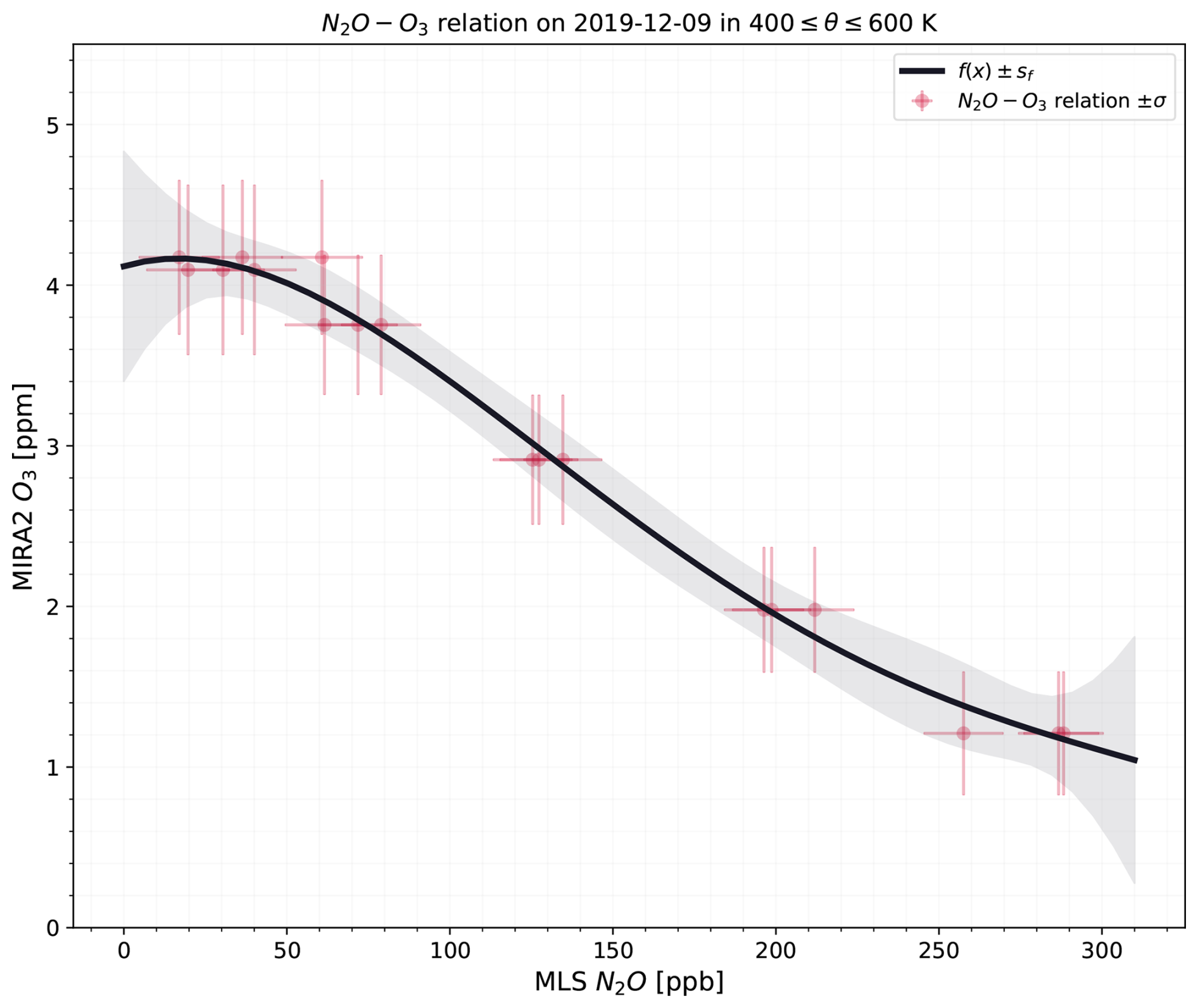
Figure 3 Relationship between MIRA2 O₃ and MLS N₂O observations between 400 and 600 K potential temperature on 9 December 2019. The solid line shows the fitted fourth-degree polynomial, while the shaded region indicates the propagated uncertainty of the fit.

The regression also provides the covariance matrix of the fitted parameters, S_f. The uncertainty of the fitted polynomial was estimated by propagating S_f using the Jacobian of Eq. (6),

$$\begin{array}{}\text{(12)}& J\left(x\right)=\left[\begin{array}{ccccc}\mathrm{1}& x& x^{\mathrm{2}}& x^{\mathrm{3}}& x^{\mathrm{4}}\end{array}\right],\end{array}$$

such that,

$$\begin{array}{}\text{(13)}& s_{\mathrm{f}}=\sqrt{J\left(x\right){\mathbf{S}}_{f}J(x{)}^T},\end{array}$$

where s_f denotes the propagated uncertainty of the fitted reference function. The observations used in the regression, together with the fitted polynomial and its associated uncertainty, are shown in Fig. 3.

The reference relationship was assumed to remain valid throughout the 2019/2020 winter season. This assumption is justified because the O₃–N₂O correlation evolves only slowly in the absence of substantial chemical ozone loss, whereas the analysis period considered here spans only a few months. However, the relationship is not expected to remain stationary on interannual timescales. Long-term changes in stratospheric ozone would for example modify the N₂O–O₃ correlation. Consequently, the reference function should be derived separately for each winter season and should not be assumed to remain valid over periods of several years.

5 Results and discussion

Before presenting the cumulative O₃ loss derived from the winter 2019/2020 MIRA2 measurements (Sect. 5.2), we first assess the consistency of the MIRA2 retrievals through comparison with coincident MLS observations.

5.1 MIRA2 and MLS comparisons

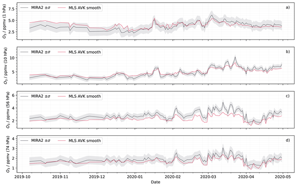
Comparisons over the full measurement period focus on four representative pressure levels (1, 10, 56, and 74 hPa; Fig. 4), selected where MIRA2 exhibits sufficient measurement response (MR). No distinction is made between air masses inside or outside the polar vortex; all coincident measurements are included to assess the robustness of the spatiotemporal coincidence criteria and the consistency of retrievals in mixed air masses. Figure 4 shows generally good agreement across all levels, with MLS typically falling within the ±σ range of MIRA2. At 56 hPa (Fig. 4c), MIRA2 slightly overestimates O₃, whereas at 1 and 10 hPa (Fig. 4a–b), a temporal shift is visible: early in the period, MIRA2 underestimates O₃, while later it overestimates. The agreement is best at 74 hPa (Fig. 4d). Overall, retrievals contain sufficient information content throughout the period.

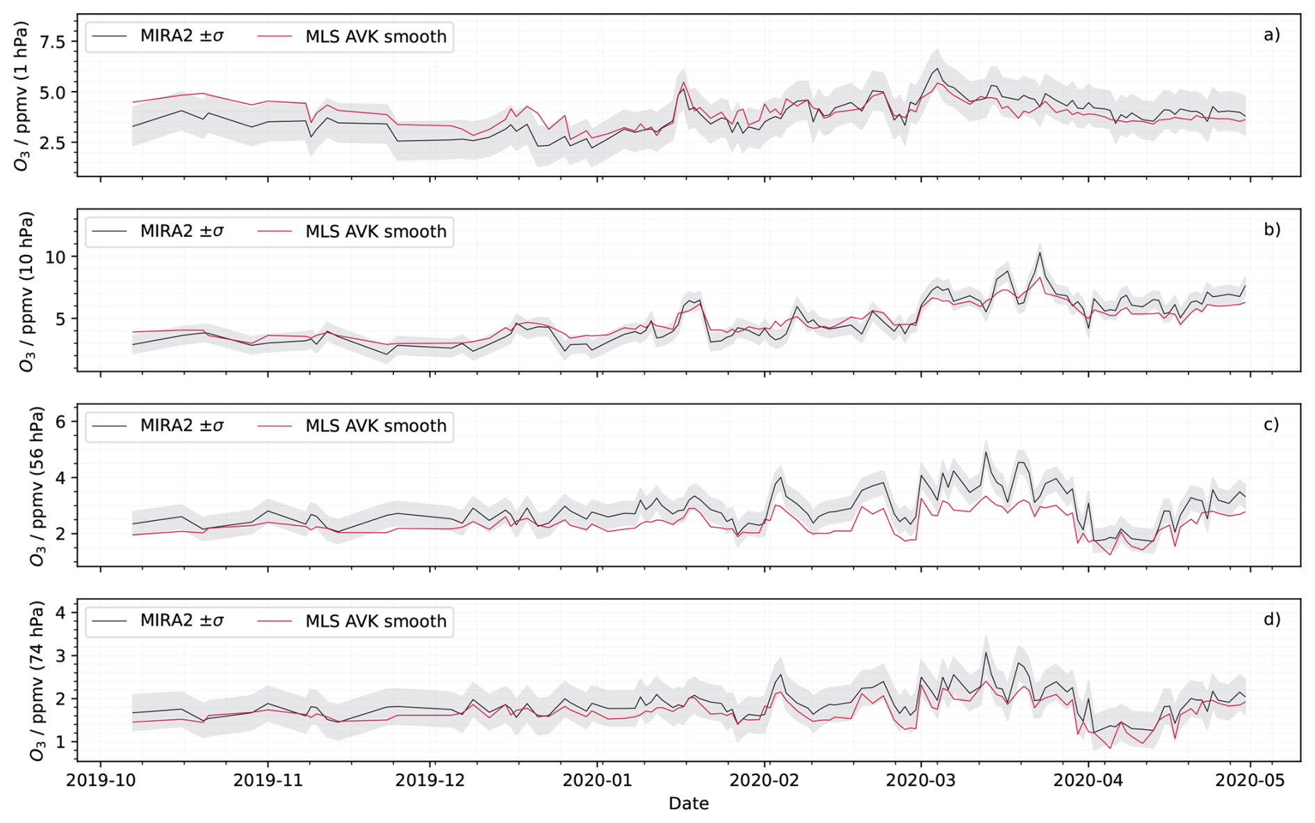
Figure 4 Comparison of coincident O₃ measurements from MIRA2 (Johansson et al., 2026) and MLS (Schwartz et al., 2020) between 1 October 2019 and 30 April 2020 at four pressure levels: 1, 10, 56, and 74 hPa (a–d). The solid black line shows MIRA2 measurements, with shaded areas indicating ±σ, reflecting total retrieval uncertainty. The solid red line shows MLS measurements smoothed with the MIRA2 averaging kernel (see Sect. 4.4).

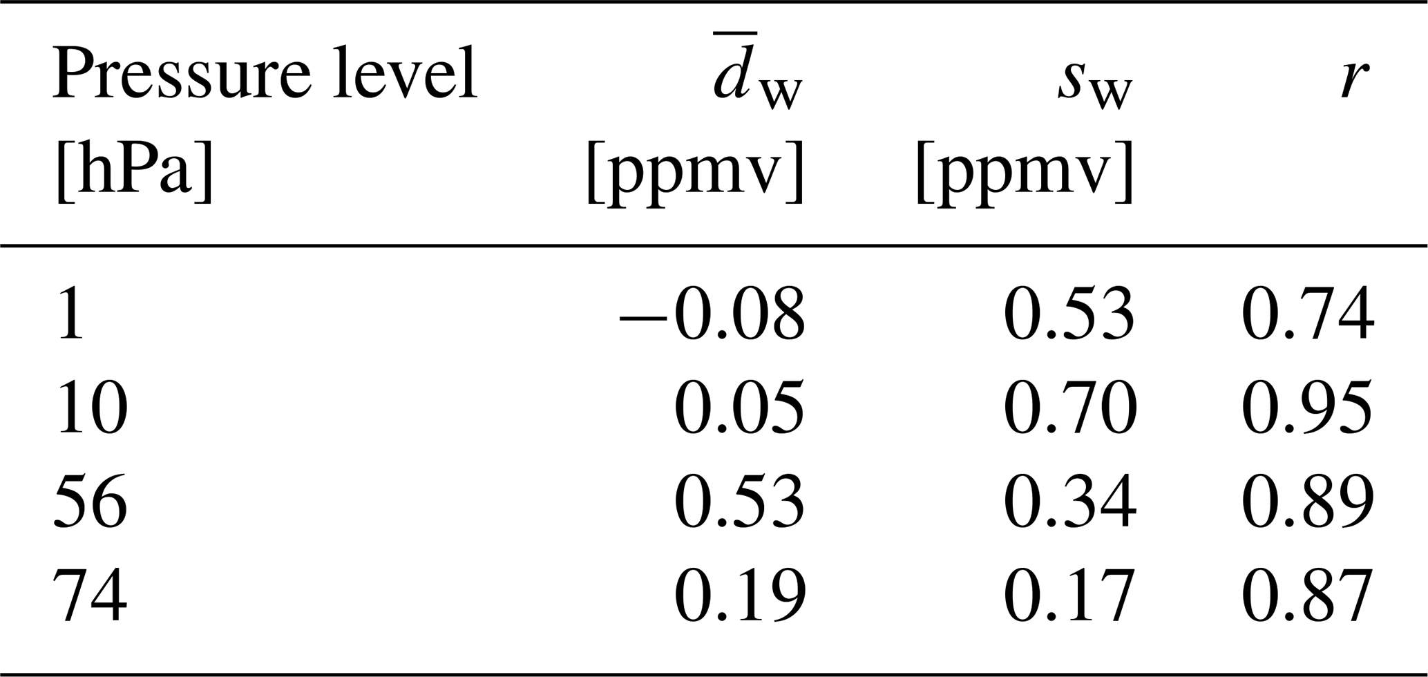
To further quantify the agreement between the two data sets, we applied a modified Bland–Altman analysis (Appendix A1) that accounts for the varying uncertainty of individual measurements. Figure 5 shows the weighted differences (MIRA2 − MLS) as a function of MLS O₃, with the weighted mean bias (${\stackrel{\mathrm{‾}}{d}}_{\mathrm{w}}$) and the limits of agreement (${\stackrel{\mathrm{‾}}{d}}_{\mathrm{w}}\pm \mathrm{1.96}{s}_{\mathrm{w}}$) indicated. The Bland–Altman analysis supports the general agreement in Fig. 4. At 1 and 10 hPa, mean differences are small (Table 1), and the majority of points lies within the 95 % limits of agreement (±1.96s_w). This provides a quantitative measure of overall agreement across the dataset. Temporal shifts are evident: MIRA2 underestimates O₃ before 15 February 2020 and overestimates it afterward. At 10 hPa, a weak magnitude-dependent bias appears, with higher MLS values being slightly overestimated by MIRA2. This could stem from a priori influence at 1 and 10 hPa, as a consequence of our approach of using a fixed O₃ a priori not adjusted over the measurement period. At 56 and 74 hPa, larger differences occur, likely due to interpolating MLS onto MIRA2's pressure grid and smoothing with the averaging kernel. Nevertheless, the majority of observations remains within the weighted limits of agreement, demonstrating overall consistency with MLS across the measurement period. Correlation analysis (Appendix A2) further supports the comparison, with linear correlation coefficients exceeding r>0.7 at all pressure levels (Table 1). Taken together, these results demonstrate that MIRA2 retrievals are internally consistent and in good agreement with MLS, providing a robust basis for subsequent ozone loss calculations.

Figure 5 Modified Bland–Altman plots showing weighted differences in O₃ (MIRA2 – MLS) at 1, 10, 56, and 74 hPa (a–d). Black points indicate observations before 15 February 2020 and red triangles after. The red line denotes the weighted mean bias ${\stackrel{\mathrm{‾}}{d}}_{\mathrm{w}}$, and the gray lines indicate the limits of agreement, ${\stackrel{\mathrm{‾}}{d}}_{\mathrm{w}}\pm \mathrm{1.96}{s}_{\mathrm{w}}$, representing the range in which 95 % of individual differences are expected to lie under an approximately Gaussian distribution (Bland and Altman, 1986).

Table 1 Summary of the statistics for the comparison between MIRA2 and MLS. ${\stackrel{\mathrm{‾}}{d}}_{\mathrm{w}}$ denotes the weighted mean difference (MIRA2 −- MLS), s_w the standard deviation of the weighted differences, and r the Pearson correlation coefficient.

5.2 Ozone loss calculations at 475 K

For the calculation of chemically induced ozone loss, we adopt potential temperature as the vertical coordinate, as described in Sect. 4.5. This choice facilitates direct comparison with previous studies of ozone depletion during winter 2019/2020 (Manney et al., 2020; Grooß and Müller, 2021). We focus our analysis on the 475 K isentropic surface (50–60 hPa), selected based on two considerations. First, MIRA2 retrievals exhibit strongest measurement response above 475 K. Second, previous studies report maximum ozone loss near 460 K (Manney et al., 2020). The 475 K level therefore represents a compromise between capturing near-maximum depletion and ensuring sufficient measurement sensitivity for a robust retrieval.

Figure 6a shows coincident daily mean ClO volume mixing ratios from MLS (Santee, 2021), while Fig. 6b (black line) presents the corresponding O₃ time series at 475 K from MIRA2. The red dots in Fig. 6b show the passive ozone (O_3P) obtained from the tracer function described in Sect. 4.6 for instances when MIRA2 measurements we obtained inside the polar vortex. The red squares in Fig. 6 show periods when the polar vortex was located over Kiruna. Due to the limited number of observations within the polar vortex, loss rates cannot be derived conclusively, neither is the period of peak loss according to the model (mid-March; Wohltmann et al., 2021) fully captured.

Figure 6 Time series of coincident mid-day ($\mathrm{12}:\mathrm{00}\pm \mathrm{2}$ h UTC) MLS ClO (Santee, 2021) (a) and MIRA2 (Johansson et al., 2026) O₃ (b) volume mixing ratio observed at the 475 K isentropic level. The black line shows daily means from MIRA2 (O_3M) and the green dots show passive ozone (O_3P) for days when measurements were obtained inside the polar vortex. Shaded regions denote ±1σ variability over the full measurement period. Dates when the polar vortex was located over Kiruna is indicated by red squares.

This limited sampling reflects a fundamental constraint of ground-based measurement at a fixed location: loosening the vortex edge criteria could introduce extra-vortex air masses into the analysis, where mixing with ozone-rich mid-latitude air would bias the derived loss toward smaller values. The selected threshold therefore represents a deliberate trade-off between sampling frequency and the representativeness of the retrieved chemical ozone loss. Nevertheless, the dataset allows estimation of cumulative ozone loss over the winter and identification of the seasonal O₃ minimum. While the temporal sampling does not fully exhibit the entire period of chemical loss, the tracer-based framework still allows following the cumulative ozone depletion, making the derived loss estimate less sensitive to data gaps in direct observations.

The temporal evolution of O₃ observed by MIRA2 (black line; Fig. 6b) shows reduced O₃ volume mixing ratio for observations within the polar vortex. This is visible already in January but most pronounced in late February and early April 2020, with the lowest O₃ observed in April 2020. MLS observations of ClO over the Kiruna area in that time period display high chlorine activation in the area, mainly in January and February, marking periods of high chemically induced ozone depletion. During intervals of observations inside the polar vortex (indicated by the red squares) increasing differences between MIRA2 ozone measurements and the passive ozone tracer values can be seen. Lowest ozone VMR has been measured by MIRA2 in early and mid April when chlorine activation no longer prevailed but other ozone depleting processes according to Wohltmann et al. (2021) still counterbalance the re-formation of ozone. The cumulative ozone loss shown in Fig. 7 (ΔO₃) is finally calculated using Eq. (11), in which the observed ozone is separated into a transport-driven component and a chemically induced loss term. While the transport-driven term, O_3P (green dots; Fig. 6b), is derived from the passive tracer reference function described in Sect. 4.6, the difference is interpreted as chemically induced ozone depletion.

Figure 7 Cumulative ozone loss (ΔO₃) at the 475 K isentropic level, derived from MIRA2 observations (Johansson et al., 2026). The loss is computed using Eq. (11) for measurements located within the polar vortex. The red star indicates the cumulative loss at 460 K reported by Manney et al. (2020), and the blue star indicates the cumulative loss at 54 hPa reported by Wohltmann et al. (2021).

Figure 7 illustrates a persistent decrease in ozone from late winter into early spring, with steeper decline from late February to April 2020. This pattern is consistent with intensified halogen-induced catalytic destruction of ozone in March 2020 reported in Wohltmann et al. (2021). The cumulative chemically induced ozone loss observed by MIRA2 reaches 2.14±0.90 ppmv at 475 K from December 2019 until the first half of April 2020. The shaded area in Fig. 7 reflects the propagated retrieval uncertainty in MIRA2 ozone observations, including measurement noise and smoothing effects.

Previous studies report maximum chemical O₃ losses of up to 2.8 ppmv below 460 K (red star in Fig. 7) (Manney et al., 2020), while near-complete depletion and minimum values of 2.5 ppmv at 54 hPa (blue star in Fig. 7) are reported by Wohltmann et al. (2021). We find that these reported peak losses are in good agreement and fall well within the estimated retrieval uncertainties of the MIRA2 results. This supports the reliability of the measurements obtained with MIRA2 and of the current retrieval. It also demonstrates that, despite the limited temporal sampling within the polar vortex, the combined use of our observations with MLS measurements enables robust characterization of both the magnitude and the seasonal evolution of Arctic ozone depletion.

6 Conclusions

In this study, ground-based microwave observations from MIRA2 were used to investigate Arctic stratospheric ozone during the winter 2019/2020 and to compare with coincident ozone observations from Aura MLS. We also quantified chemical ozone loss on isentropic surfaces from MIRA2 observations.

Comparison with coincident MLS measurements shows that MIRA2 retrievals are consistent across the investigated pressure levels, with rather small biases and without statistically significant differences. This agreement demonstrates that MIRA2 provides reliable ozone measurements with sufficient information content for quantitative analysis of stratospheric variability.

Using a tracer-based framework, cumulative chemically induced ozone loss was derived at the 475 K isentropic level. The results show a steady increase in ozone loss from late winter into early spring, reaching 2.14±0.90 ppmv in early April 2020. The timing and magnitude of the loss are consistent with the exceptional Arctic ozone depletion reported by other studies.

The observed temporal offset between peak ClO and minimum O₃ highlights the cumulative nature of chemical ozone loss and reflects the evolution of chlorine activation and deactivation within the polar vortex. This behavior is consistent with the established understanding of halogen-driven ozone depletion under cold and sunlit conditions in air-masses confined within a long lasting polar vortex.

Despite limited temporal sampling of vortex air masses, the tracer-based approach enables reconstruction of seasonal ozone loss, reducing sensitivity to observational gaps. This demonstrates the capability of ground-based microwave radiometers to capture both the magnitude and temporal evolution of Arctic ozone depletion events.

Overall, this study shows that MIRA2 provides consistent and reliable stratospheric ozone retrievals, in good agreement with MLS and previous analyses of the 2019/2020 Arctic winter. Combining data from MIRA2 with MLS allows the construction of tracer–tracer relationships and the temporal and spatial identification of polar vortex air masses, demonstrating the value of direct observational data for quantifying chemical ozone loss. These results highlight the critical role of comprehensive measurements in capturing stratospheric variability, while also revealing the current reliance on a limited set of observing systems. As MLS approaches the end of its operational lifetime, maintaining and expanding alternative observational capabilities is essential. This expansion should include more measurements of tracers relevant to stratospheric chemistry, reducing reliance on model assumptions and strengthening observational constraints on ozone variability and recovery.

Appendix A: Statistics

A1 Weighted Bland–Altman analysis

We compare coincident daily mean measurements from MIRA2 (G_i) and MLS (S_i) using a weighted Bland–Altman approach, where individual differences are weighted by their combined uncertainty. Pointwise uncertainties from MIRA2 and MLS are assumed independent:

$$\begin{array}{}\text{(A1)}& {\mathit{\sigma }}_{C_i}=\sqrt{{\mathit{\sigma }}_{G_i}^{\mathrm{2}}+{\mathit{\sigma }}_{S_i}^{\mathrm{2}}}.\end{array}$$

For each coincident pair:

$$\begin{array}{}\text{(A2)}& {\displaystyle }{M}_i={\displaystyle \frac{G_i+S_i}{\mathrm{2}}},\text{(A3)}& {\displaystyle }{D}_i=G_i-S_i.\end{array}$$

The weight for each observation is the inverse of the squared combined uncertainty:

$$\begin{array}{}\text{(A4)}& w_i={\displaystyle \frac{\mathrm{1}}{{\mathit{\sigma }}_{C_i}^{\mathrm{2}}}}.\end{array}$$

The weighted mean difference (bias) is:

$$\begin{array}{}\text{(A5)}& {\stackrel{\mathrm{‾}}{d}}_{\mathrm{w}}={\displaystyle \frac{{\sum }_i{w}_i{D}_i}{{\sum }_i{w}_i}},\end{array}$$

and the weighted variance of differences is

$$\begin{array}{}\text{(A6)}& s_{\mathrm{w}}^{\mathrm{2}}={\displaystyle \frac{{\sum }_i{w}_i(D_i-{\stackrel{\mathrm{‾}}{d}}_{\mathrm{w}}{)}^{\mathrm{2}}}{{\sum }_i{w}_i-\frac{{\sum }_i{w}_i^{\mathrm{2}}}{{\sum }_i{w}_i}}}.\end{array}$$

Assuming approximate Gaussianity, the 95 % limits of agreement are defined as

$$\begin{array}{}\text{(A7)}& \mathrm{LoA}={\stackrel{\mathrm{‾}}{d}}_{\mathrm{w}}\pm \mathrm{1.96}{s}_{\mathrm{w}}.\end{array}$$

These limits provide a practical range in which 95 % of individual differences are expected to lie, incorporating both systematic bias and random variability while accounting for measurement uncertainties that vary across observations (Bland and Altman, 1986; Myles and Cui, 2007).

A2 Correlation analysis

To complement the Bland–Altman analysis, we evaluated the linear relationship between coincident O₃ measurements from MIRA2 and MLS using the Pearson correlation coefficient, r. For paired observations {G_i,S_i}, the Pearson r is defined as

$$\begin{array}{}\text{(A8)}& r={\displaystyle \frac{{\sum }_i(G_i-\stackrel{\mathrm{‾}}{G})(S_i-\stackrel{\mathrm{‾}}{S})}{\sqrt{{\sum }_i(G_i-\stackrel{\mathrm{‾}}{G}{)}^{\mathrm{2}}}\sqrt{{\sum }_i(S_i-\stackrel{\mathrm{‾}}{S}{)}^{\mathrm{2}}}}},\end{array}$$

where $\stackrel{\mathrm{‾}}{G}$ and $\stackrel{\mathrm{‾}}{S}$ are the sample means of the MIRA2 and MLS measurements, respectively.

Pearson r quantifies the strength and direction of the linear association between the two datasets, with r=1 indicating perfect positive linear correlation, r=0 indicating no linear correlation, and $r=-\mathrm{1}$ indicating perfect negative linear correlation. The statistical significance of r can be assessed under the null hypothesis of no correlation.

Pearson correlation coefficients are widely used in atmospheric remote sensing intercomparisons to assess the consistency of co-located measurements (Steinbrecht et al., 2009; Tummon et al., 2015). While high s does not imply perfect agreement in magnitude (see related bias and limits of agreement in Appendix A1), it adds confidence that the temporal and vertical variability observed by MIRA2 is consistent with MLS observations.

Appendix B: Reference function coefficients

The coefficients a_i of the reference function defined in Eq. (6) are provided in Table B1. The sample means and standard deviations used for the normalization in Eqs. (7)–(10) are provided in Table B2.

Table B1 Coefficients a_i of the reference function defined in Eq. (6).

Table B2 Sample means and standard deviations used for the normalization in Eqs. (7)–(10).