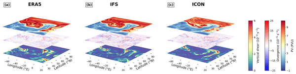
Evidence of gravity wave contribution to vertical shear and mixing in the lower stratosphere

Small-scale dynamics, particularly gravity waves (GWs), modify vertical wind shear and can trigger turbulence in the lowermost stratosphere (LMS), thereby influencing the transport of trace species across the tropopause. Although idealized modeling and observational case studies have demonstrated this link, the contribution of small-scale dynamics to turbulence generation remains poorly understood, particularly under real atmospheric conditions. Here, we investigate the relationship between GWs, vertical wind shear, and clear-air turbulence (CAT) in the LMS over the North Atlantic during a baroclinic life cycle. We combine airborne observations with ERA5 reanalysis and high-resolution forecasts from the IFS and ICON models. To isolate the contribution of small-scale dynamics to turbulence generation, we extract the small-scale divergent component of the modeled wind field. From this, we derive momentum flux, perturbation vertical wind shear, and the turbulence indices TI1 and TI2, and compare these quantities with those calculated from the full wind fields. Trace-species mixing is observed within a region of enhanced GW activity over Iceland that is characterized by increased vertical wind shear and turbulence. ERA5 reproduces the spatial and temporal distribution of enhanced shear and turbulence but underestimates shear magnitudes relative to the forecasts while yielding comparable values of TI1 and TI2. These findings extend previous idealized studies from Umbarkar and Kunkel (2025) to real atmospheric conditions and provide further evidence that GW-induced small-scale dynamics contribute to turbulence generation in the LMS. They also demonstrate the potential of ERA5 for long-term investigations of the role of small-scale dynamics in transport and mixing near the tropopause.

1 Introduction

Atmospheric gravity waves (GWs), ubiquitous buoyancy-driven oscillations, play a crucial role in a wide range of atmospheric processes. They can initiate and organize convection (Zhang et al., 2001) as well as generate and modulate atmospheric turbulence (Shapiro, 1980). By propagating vertically, GWs redistribute momentum and energy, thereby influencing the general circulation, particularly in the upper atmosphere, as well as the exchange of air masses between the troposphere and stratosphere (Holton et al., 1995).

Generally, GWs are generated by topographic forcing, convection, shear instability, and geostrophic adjustment associated with jets, fronts, and regions of strong diabatic heating (Hooke, 1986; Fritts and Alexander, 2003; Kim et al., 2003; Plougonven et al., 2008). Orographic GWs arise from the interaction of atmospheric flow with topographic features, producing predominantly vertically propagating waves that influence the energy and momentum budget of the UTLS (Durran, 1995; Lachnitt et al., 2023). They propagate into the stratosphere, where they dissipate and modify the atmospheric circulation, particularly the Brewer–Dobson circulation (Achatz et al., 2024, and references therein). Convectively generated GWs result from latent heat release and rapid vertical motions, such as those occurring in thunderstorms, and are commonly observed in both tropical and extratropical regions (Fritts and Alexander, 2003; Alexander et al., 2010). Moreover, Lane et al. (2001) and Lane and Sharman (2006) showed that GWs are generated when convective updrafts rapidly decelerate. The spatial distribution and relative importance of GW sources largely determine the global GW climatology and, consequently, their influence on atmospheric stability and transport processes.

In the extratropics, baroclinic life cycles represent an important, albeit less well understood, source of GWs. They exhibit fine-scale substructures, including upper- and lower-level fronts, convective ascent, jet streaks and regions of flow imbalance that can excite GWs through spontaneous imbalance, whereby departures from balanced flow trigger wave emission (Plougonven and Zhang, 2014; Zhang et al., 2015b). Regions of baroclinic instability, particularly along jet streaks and frontal zones, are hotspots of non-orographic GW activity. Furthermore, tropospheric moist processes play an important role in the generation of GWs by mid- and high-latitude weather systems (e.g., Wei and Zhang, 2014; Plougonven et al., 2015; Holt et al., 2017). In these regions, interactions between divergent flow associated with GWs and the background flow (Trier et al., 2020) enhance vertical shear and promote turbulence (e.g., O'Sullivan and Dunkerton, 1995; Plougonven and Snyder, 2005; Zülicke and Peters, 2006; Kaluza et al., 2021). GWs generated by tropospheric weather systems (or synoptic eddies) can propagate into the UTLS and middle atmosphere, where they deposit momentum and energy upon dissipation, thereby contributing to the Brewer–Dobson circulation (Alexander et al., 2010; Achatz et al., 2024, and references therein). Around the tropopause, GWs generated by baroclinic systems also modify the dynamic and thermodynamic structure of the UTLS (Plougonven et al., 2008; Dörnbrack, 2024; Jovanovic, 2025). Despite their ubiquity, however, the generation mechanisms of these GWs remain poorly understood.

Besides baroclinic systems, orographic GWs, despite their pronounced seasonality and transient nature, frequently induce turbulence near the tropopause (Fritts and Alexander, 2003; Alexander and Grimsdell, 2013; Rapp et al., 2021). For example, Lachnitt et al. (2023) showed that GW-induced turbulence can persistently alter the distribution of trace species in the lower stratosphere. These processes modify the isentropic gradients of radiatively active trace species (e.g., Dörnbrack et al., 2025) and thereby contribute to the mixing-induced uncertainty in radiative forcing (Riese et al., 2012).

GWs induce fluctuations of key state variables within the background flow and thereby affect vertical wind shear and static stability in the tropopause region (Kunkel et al., 2016; Kaluza et al., 2021; Dörnbrack, 2024). When GWs dissipate or break, these initially reversible fluctuations can result in irreversible mixing and GW momentum flux convergence, which modifies the background state on longer time scales. Ultimately, this process can contribute to the formation of an enhanced shear layer in the extratropics, known as the tropopause shear layer (TSL, Kaluza et al., 2021). The TSL is typically identified as the region near the extratropical tropopause where shear exceeds a critical threshold $S_{\mathrm{t}}^{\mathrm{2}}$, often defined as the 95th percentile of climatological dataset. Such enhanced shear is often linked to tropopause disturbances and has been observed on the order of 10⁻²–${\mathrm{10}}^{-\mathrm{3}}{\mathrm{s}}^{-\mathrm{1}}$ (Lane et al., 2004; Kaluza et al., 2021). It occurs particularly in dynamically active regions, such as jet streaks and frontal zones and often in combination with clear air turbulence (Koch et al., 2005; Wang and Zhang, 2007). Additionally, large vertical shear in the lower stratosphere is often accompanied by enhanced static stability. This increase is partly attributed to the effects of GW dissipation in this region (Kunkel et al., 2014; Zhang et al., 2015b). Analysis of aircraft observations and model simulations have further demonstrated that irreversible mixing occurs in these regions (Kunkel et al., 2019). However, such analyses remain limited due to sparse observational data sets and the requirement for very high resolution models to correctly capture the relevant processes (Plougonven and Zhang, 2014; Stephan et al., 2019a; Geller et al., 2013; Jewtoukoff et al., 2015).

GWs influence tracer transport and mixing in the UTLS by generating turbulence, either through enhanced vertical shear that triggers instabilities such as Kelvin–Helmholtz instability or through wave breaking at critical levels where the GW phase speed matches the background wind (e.g., Shapiro, 1978; Whiteway et al., 2004; Lane and Sharman, 2006). Consequently, GWs can contribute to the formation of the extratropical transition layer (ExTL), a region surrounding the extratropical tropopause that, from a tracer-based perspective, represents the transition between stratospheric and tropospheric air masses (Hoor et al., 2004; Pan et al., 2006; Hegglin et al., 2009). The ExTL is largely confined to the lower part of the lowermost stratosphere (LMS). While the ExTL is located around the extratropical tropopause, typically defined by a potential vorticity isosurface, the LMS extends between the extratropical and tropical tropopause and is bounded above by the 380 K isentrope (Appenzeller et al., 1996; Holton et al., 1995; Olsen et al., 2013; Wang and Fu, 2021; Weyland et al., 2025). Trace species originating in the troposphere, such as water vapor and carbon monoxide, or in the stratosphere, such as ozone, exhibit pronounced vertical gradients across the ExTL and LMS. These gradients reflect the distribution of source regions, chemical transformations, and transport and mixing processes in the troposphere and stratosphere. In the extratropics, quasi-isentropic transport plays a key role in exchanging air masses between the troposphere and stratosphere and within the stratosphere, as demonstrated by trajectory analyses (Berthet et al., 2007; Hoor et al., 2010) and airborne observations (e.g., Hoor et al., 2004; Pan et al., 2004; Kunkel et al., 2019). In addition, small-scale processes promote more localized mixing, often in association with shear instabilities or convection (e.g., Whiteway et al., 2003; Lane et al., 2004; Zhang et al., 2015b; Lachnitt et al., 2023; Dörnbrack et al., 2025). Consequently, the composition of the ExTL is influenced by GW-induced transport and mixing, which in turn affect the radiative balance of the extratropical UTLS (Birner et al., 2002; Birner, 2006; Hoor et al., 2004; Zhang et al., 2015a; Heller et al., 2017).

A particularly important manifestation of GW-induced turbulence in the lower stratosphere is shear-induced clear-air turbulence (CAT). Identifying CAT is crucial for aviation safety and for understanding the mixing of trace species and, consequently, the chemical composition of the UTLS (Chau et al., 2025, 2026). Simulations of midlatitude cyclones have highlighted the role of jet dynamics and GWs in the generation of CAT (Lane et al., 2004; Trier et al., 2020). In addition to vertical shear-based diagnostics, such as the gradient Richardson number, empirical turbulence indices including TI1 and TI2 are widely used to identify CAT (Ellrod and Knapp, 1992; Sharman et al., 2006; Jaeger and Sprenger, 2007). However, forecasting CAT remains challenging because of its intermittent nature and small spatial scales, with turbulent eddies typically spanning horizontal scales of only ∼ 10–1000 m, far below the resolution of current numerical weather prediction models (Sharman et al., 2006, 2014; Sharman and Pearson, 2017). Therefore, improving our understanding of the processes that generate CAT is essential, particularly since GW activity and enhanced vertical shear are key factors promoting its development.

This study is motivated by recent findings from idealized simulations of baroclinic life cycles (Umbarkar and Kunkel, 2025), which revealed a clear relationship between GWs, enhanced vertical shear, and turbulence in the lower stratosphere. Here, we investigate whether this relationship is also evident during an extratropical baroclinic life cycle over the North Atlantic. First, we present observational evidence of recent mixing between chemically distinct air masses during a flight of the WISE (Wave-driven ISentropic Exchange) mission in September 2017 and examine whether this mixing event is associated with enhanced vertical shear and GW activity (Sect. 3). We then analyse the representation of vertical shear and the associated GW-induced turbulent mixing in ERA5 reanalysis over the North Atlantic during this event (Sect. 4). Subsequently, we compare the ERA5 results with IFS forecasts and ICON simulations at different horizontal resolutions (Sect. 5) to assess which characteristics of the GW field can be reliably represented by ERA5, given its spatial resolution, and whether the resolved GW spectrum is sufficient to investigate GW impacts on shear and mixing in the UTLS in case studies and, ultimately, in climatological analyses. Finally, we examine whether instabilities triggered by GW-induced shear can lead to the development of CAT.

2 Data and methods

2.1 In situ measurements

In autumn 2017, the WISE (Wave-driven ISentropic Exchange) campaign was conducted using the German HALO (High Altitude and Long Range) research aircraft, with flight operations based in Oberpfaffenhofen, Germany, and Shannon, Ireland. In this study we focus on research flight 05 on 23 September 2017 between 08:09 and 17:04 UTC, further denoted as RF05. The goal of this flight was to investigate the dynamical and chemical structure of the atmosphere in the vicinity of the tropopause over the North Atlantic between Ireland and a subtropical intrusion extending far north of Iceland.

During the WISE campaign, HALO was equipped with a comprehensive suite of instruments for in situ and remote sensing. Our analysis is mainly based on in-situ measurement of CO and N₂O from UMAQS (University of Mainz Airborne Quantum Cascade Laser Spectrometer,  Müller et al., 2015). For the WISE campaign, the total drift-corrected uncertainty was determined to be 0.94 ppbv for CO and 0.18 ppbv for N₂O (Kunkel et al., 2019). Additionally, we use meteorological parameters measured with BAHAMAS (Basic HALO Measurement and Sensor System, Krautstrunk and Giez, 2012; Kunkel et al., 2019).

2.2 ERA5 reanalysis data

As a reference for the zonal and meridional wind components and to provide the meteorological context for our analysis, we use ERA5, the fifth-generation atmospheric reanalysis produced by the European Centre for Medium-Range Weather Forecasts (ECMWF) (Hersbach et al., 2020). ERA5 is based on four-dimensional variational (4D-Var) data assimilation using cycle Cy41r2 of the ECMWF Integrated Forecasting System (IFS). The reanalysis is available on 137 model levels extending from the surface to 0.01 hPa, with a vertical grid spacing of approximately 300 m in the UTLS. For our analysis, the model-level data were additionally interpolated onto height, pressure, and isentropic coordinates. We use two ERA5-based datasets: (i) meteorological fields extracted along the HALO flight track, which are analysed in Sect. 3 (Lachnitt, 2025), and (ii) four-dimensional meteorological fields with hourly temporal resolution on a 0.25° × 0.25° latitude–longitude grid, which are used in Sect. 4.

2.3 IFS forecast

Next, we use ECMWF IFS operational forecast data as a high resolution complement of the ERA5 reanalysis. The data are based on IFS cycle 43r3 and are provided on a regular 0.1° latitude-longitude grid with hourly temporal resolution. This dataset is particularly suitable for this study because the IFS version used to produce this forecast is closely related to the version employed for the production of ERA5. The operational IFS employs a Tco1279 spectral truncation and an associated O1280 octahedral grid, resulting in a horizontal grid spacing of approximately Δx≈ 9 km. It incorporates 137 vertical levels, corresponding to the same vertical resolution used in both ERA5 and forecasts. The operational forecast therefore shares a similar dynamical core and physical parameterizations with ERA5, allowing the impact of increased horizontal resolution on the representation of shear and GWs to be investigated. We use the operational forecast from 23 September 2017 00:00 UTC, with hourly resolution for the first 24 h of this forecast.

2.4 ICON forecast

In addition, we use forecast data of this case from Schwenk and Miltenberger (2024), who employed version 2.6.2 of the ICOsahedral Nonhydrostatic (ICON) modeling framework (Zängl et al., 2014) over the North Atlantic Ocean. This enables us to study the representation of the same situation in a model with a different dynamical core and physics package, as well as across three different resolutions ranging from approximately the resolution of the IFS data to near convection-permitting scales. This allows us to directly assess the robustness of our findings across different model representations.

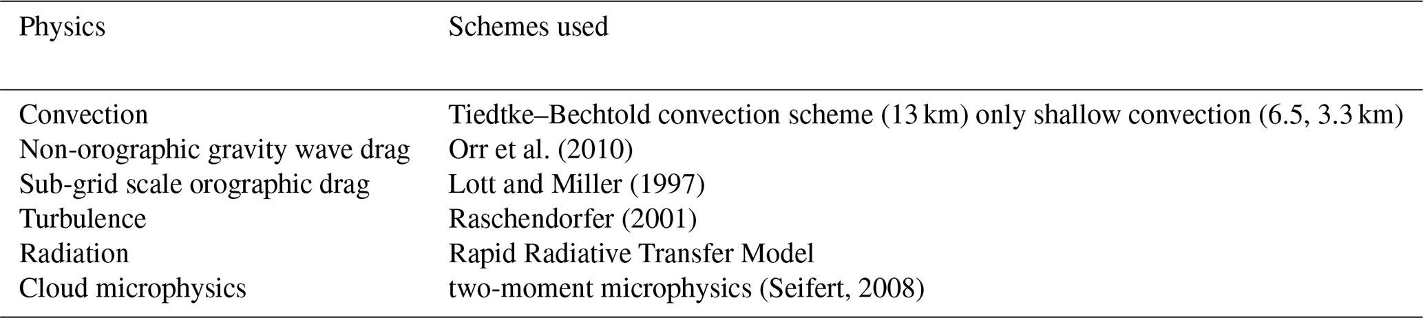
The simulation was initialized with the operational global ICON analysis at 00:00 UTC on 20 September 2017, shortly before the cyclone developed, and integrated for 96 h until 00:00 UTC on 24 September 2017, when the cyclone life cycle was in its final stage (Schwenk and Miltenberger, 2024). The global ICON model simulation used an R03B07 grid (effective resolution of ∼ 13 km) with a 120 s time step and included nested regions using R03B08 (6.5 km) and R03B09 (3.3 km) grids with time steps of 60 and 30 s, respectively (Fig. A3). Vertically, the ICON simulations comprise 90 levels from the surface to 23 km altitude, with a grid spacing of approximately 250–300 m in the UTLS. Figure 1 illustrates the ICON nested configuration and the atmospheric situation over the study region based on ERA5 at 11:00 UTC on 23 September 2017. Further details on the physics parameterization schemes used in the ICON simulations are provided in Table 1.

Orr et al. (2010)Lott and Miller (1997)Raschendorfer (2001)(Seifert, 2008)

Table 1 Summary of physics parameterization schemes used for ICON simulations

2.5 Deriving resolved gravity wave momentum fluxes and turbulence diagnostics

For the analysis of GWs and turbulence using model fields, we follow the approach outlined in Umbarkar and Kunkel (2025), with some extensions. We briefly outline the most important aspects here. First, GWs manifest themselves as small–scale deviations from the background state. We therefore use a hybrid method that combines a dynamical with a statistical approach to separate the (large–scale) background from the (small–scale) deviations (similar to Wei et al., 2022). Note that we define the large–scale flow as the background state in this context.

We first decompose the flow into its divergent and rotational components using a Helmholtz decomposition, i.e., the dynamical approach. For the statistical component, we then apply a spectral filter using a one-dimensional zonal Fast-Fourier Transformation (FFT) over the full domain shown in Fig. 1. In this step, we remove contributions from wavenumbers 0 to 20, i.e. $u^{\prime }=u_{\text{div}}-{\left(u_{\text{div}}\right)}_{k\le k_{\mathrm{s}}}$, where k_s=20, is the wavenumber cutoff separating the respective quantities into large–scale and small–scale components. The primes (^′) denote deviations from the background state throughout the remainder of this study. Sensitivity tests with k_s values of ±4 showed no significant variations in the resulting primed quantities. The deviations of the small–scale flow from large–scale background flow are shown in Fig. A1.

We identify GWs once based on the horizontal divergence ∇_h⋅u_h (e.g.,  Kunkel et al., 2014). Additionally, we use the absolute momentum flux

$$\begin{array}{}\text{(1)}& \mathrm{AMF}=\mathit{\rho }\sqrt{(\stackrel{\mathrm{‾}}{u^{\prime }{w}^{\prime }}{)}^{\mathrm{2}}+(\stackrel{\mathrm{‾}}{v^{\prime }{w}^{\prime }}{)}^{\mathrm{2}}}\end{array}$$

where ρ is the mean density, and u^′, v^′, and w^′ are the zonal, meridional, and vertical velocity perturbations, respectively. The overline over the perturbation products (i.e. $\stackrel{\mathrm{‾}}{u^{\prime }{w}^{\prime }}$ and $\stackrel{\mathrm{‾}}{v^{\prime }{w}^{\prime }}$) highlights a low-pass filtering of the quadratic quantities using the same Gaussian spectral filter as in Kruse and Smith (2015). We use the AMF as a first proxy for the momentum flux due to small-scales and as such to GWs.

A recent study by Zhang et al. (2025) suggests that the hybrid scale-separation approach is applicable in the LMS (e.g., around 200 hPa). Moreover, Wei et al. (2022) and Zhang et al. (2025) further demonstrate that using the divergent wind to separate the GW component from the background provides more reliable estimates of GW momentum flux, particularly in the upper troposphere. Thus, we emphasize that our hybrid approach for separating the flow scales is well justified in the UTLS (Zhang et al., 2025) and follows commonly used GW scale-separation methods (Lehmann et al., 2012; Wei et al., 2016; Stephan et al., 2019a; Strube et al., 2020; Gupta et al., 2021; Wei et al., 2022; Umbarkar and Kunkel, 2025), despite different cutoff wavenumber used among these studies. Nevertheless, the focus in this study is primarily on the LMS, where the separation between large-scale and small-scale motions is comparatively more robust and the limitations of the method are therefore reduced.

We use several other quantities to analyze whether the flow is prone to turbulence occurrence. A key diagnostics is the vertical shear:

$$\begin{array}{}\text{(2)}& S^{\mathrm{2}}={\left({\displaystyle \frac{\partial u}{\partial z}}\right)}^{\mathrm{2}}+{\left({\displaystyle \frac{\partial v}{\partial z}}\right)}^{\mathrm{2}}.\end{array}$$

While S² is derived from the full wind field, it is also calculated from the wind perturbations, further denoted as $S^{{\mathrm{2}}^{\prime }}$. Furthermore, we use the gradient Richardson number Ri and the Ellord turbulence indices, TI1 and TI2, to estimate whether the flow is turbulent (Sharman et al., 2006). The use of multiple diagnostics is motivated by the need to capture both the dynamical and kinematic aspects of turbulence generation in the extratropical UTLS, especially in regions affected by GW-induced shear and mixing. Here, dynamical diagnostics characterize the stratification of the flow and its susceptibility to instabilities, whereas kinematic diagnostics describe flow deformation and shear processes that can promote turbulence development. Ri is calculated as follows:

$$\begin{array}{}\text{(3)}& Ri={\displaystyle \frac{N^{\mathrm{2}}}{S^{\mathrm{2}}}}={\displaystyle \frac{\left(\frac{g}{\mathit{\theta }}\frac{\partial \mathit{\theta }}{\partial z}\right)}{{\left(\frac{\partial u}{\partial z}\right)}^{\mathrm{2}}+{\left(\frac{\partial v}{\partial z}\right)}^{\mathrm{2}}}}\end{array}$$

i.e., the ratio of static stability (N²) to vertical wind shear (S²). It is commonly assumed that a Richardson number below a critical value is required for a Kelvin-Helmholtz instability to occur. The critical value for linear shear instability of an idealized stratified flow is often determined to be 0.25; however, for model based analyses values on the order of 1 are considered indicative of regions susceptible to Kelvin-Helmholtz instabilities (e.g., Kunkel et al., 2019). Note that the total vertical wind shear is used to compute Ri in order to initially evaluate regions susceptible to turbulence within the baroclinic flow.

In addition to Ri, we use the Ellord-Knapp turbulence indices, TI1 and TI2, which are empirical diagnostics specifically developed to identify CAT, to better represent turbulence under complex flow conditions. The TI1 has previously been shown to be capable of detecting 70 %–84 % of CAT occurrences (e.g., Ellrod and Knapp, 1992; Sharman and Pearson, 2017; Kim et al., 2018; Gultepe et al., 2019; Thompson and Schultz, 2021). We resort this to the small–scales, ensuring that potential turbulence in the subsequent analysis reflects subgrid or small–scale contributions. We note here that Kelvin-Helmholtz instability and turbulence are not explicitly resolved in the reanalyses and forecasts even if the GWs themselves are. While these processes are represented through subgrid-scale parameterizations, our analysis uses diagnostics based on the resolved fields in ERA5, IFS and ICON. These diagnostics highlight regions with favourable conditions for turbulence occurrence. Following Ellrod and Knapp (1992), the TI1 combines vertical wind shear perturbations and the total flow deformation (DEF), whereas TI2 adds additionally a convergence (CVG) term. The TI1 is calculated as

$$\begin{array}{}\text{(4)}& \text{TI1}=S\times \text{DEF}\end{array}$$

and the TI2 as:

$$\begin{array}{}\text{(5)}& \text{TI2}=S\times (\text{DEF}+\text{CVG})\end{array}$$

where (S) is the magnitude of vertical wind shear perturbations ($S^{{\mathrm{2}}^{\prime }}$, see Eq. 2). DEF is the total flow deformation:

$$\begin{array}{}\text{(6)}& \text{DEF}={\left({\left({\displaystyle \frac{\partial u}{\partial x}}-{\displaystyle \frac{\partial v}{\partial y}}\right)}^{\mathrm{2}}+{\left({\displaystyle \frac{\partial v}{\partial x}}+{\displaystyle \frac{\partial u}{\partial y}}\right)}^{\mathrm{2}}\right)}^{\mathrm{1}/\mathrm{2}}\end{array}$$

and convergence is calculated according to,

$$\begin{array}{}\text{(7)}& \text{CVG}=-\left({\displaystyle \frac{\partial u}{\partial x}}+{\displaystyle \frac{\partial v}{\partial y}}\right)\end{array}$$

Here, both CVG and DEF are consistently derived from the perturbation wind components (u^′, v^′), and thus TI1 and TI2 are likewise based only on the corresponding prime quantities. The inclusion of CVG in TI2 offers an advantage over TI1 by capturing the small–scale flow features such as those associated with GWs or upper level frontal structures. These region often exhibit enhanced shear and convergence making TI2 more sensitive to turbulence driven by small–scale processes.

3 Analysis of GW induced mixing in a baroclinic wave over Iceland

3.1 Meteorological situation

The major goal of the flight was to determine whether trace species exhibit specific signatures of irreversible mixing in regions of enhanced static stability in the lower stratosphere. We use this flight dataset and further investigate whether this irreversible mixing event occurs in regions of GW-induced shear enhancement. The flight was conducted within the ridge of a synoptic-scale baroclinic wave which developed over the North Atlantic during the preceding days, at the edge of large–scale trough.

The isentropic distribution of potential vorticity at 340 K in Fig. 1 illustrates the meteorological situation during WISE RF05 for ERA5 reanalysis fields. The synoptic situation over the North Atlantic Ocean on 23 September 2017 at 11:00 UTC is dominated by a strong meridional excursion of subtropical air masses far northward, extending from the Iberian Peninsula over Great Britain to Iceland. Adjacent to the tropospheric streamer two equatorward reaching stratospheric streamers are present, the one to the west being more coherent in its structure, while the one to the east shows more internal structure in terms of its isentropic PV.

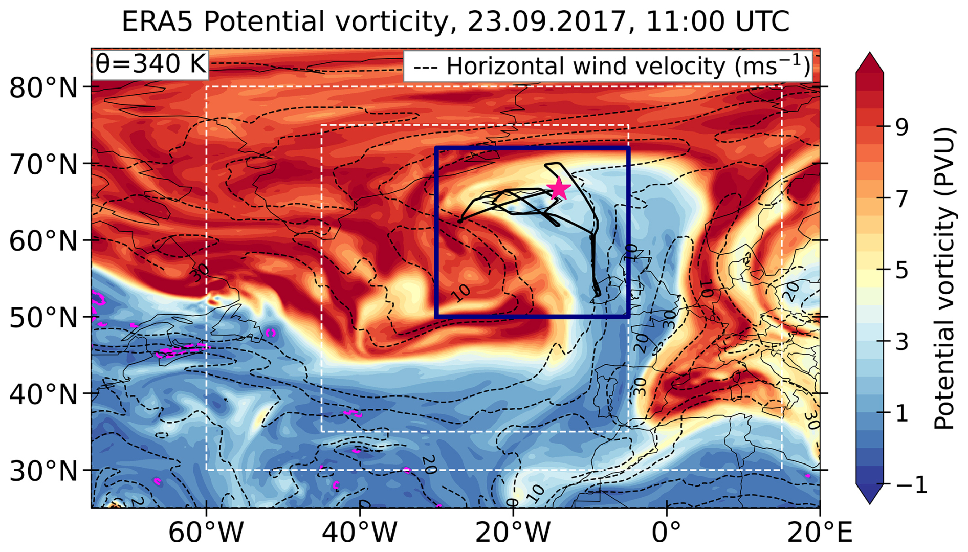
Figure 1 Potential vorticity distribution (in PVU) at the 340 K isentropic surface on 23 September 2017 at 11:00 UTC for ERA5 reanalysis data. The dashed lines show the horizontal wind (in m s⁻¹) at 340 K. The thick black line shows the flight path of research flight 05 and the star marks the aircraft position at 11:00 UTC. Magenta color shows negative PV values which are often related to cloud processes.

The flight was conducted from Shannon, Ireland, towards Iceland, where a hexagon pattern was flown and a dive was performed before returning to Shannon (see black line in Fig. 1). The PV distribution shows that the flight took place predominantly within the region where subtropical air masses at around 11–13 km were transported poleward, while some parts of the flight track also crossed the PV gradient into the lower stratosphere. The region of the strong PV gradient corresponds to the location of the jet stream and acts as a barrier between tropospheric and stratospheric air masses. On the large–scale, IFS (Fig. A2) and ICON (Fig. A3) forecasts show similar patterns in terms of the overall PV distribution. Moreover, smaller scale, ripple-like structures in the PV field around 20° W and 65° N (Fig. 1) could indicate wave activity similar to the another case during WISE (Kunkel et al., 2019). Such small–scale structures in the PV field may already hint at the presence of GWs associated with air-mass mixing.

3.2 Identification of flight segments affected by turbulence

Next, we examine the time series of measured and ERA5 derived quantities during WISE RF05. The goal is to identify regions and periods of potential turbulence and small–scale mixing above the tropopause.

Figure 2 shows a comparison of in situ measured atmospheric state parameters, including chemical tracers and potential temperature (a), and instability parameters (b) from the ERA5 reanalysis data interpolated in time and space onto the flight path. The pressure altitude measured during WISE RF05 indicates that the flight path was designed to ascend with time (Fig. 2a), with the exception of the dive between 13:00 and 14:00 UTC. This ascent is also reflected in the decrease of N₂O with time and the corresponding increase in potential temperature and ERA5 PV. In contrast, ERA5 vertical shear S² and Richardson number Ri exhibit a more variable temporal evolution. In particular, two shear maxima are evident, reaching values up to $\mathrm{8}\times {\mathrm{10}}^{-\mathrm{4}}{\mathrm{s}}^{-\mathrm{2}}$, which are associated with minima in Ri below 1 (Fig. 2b). Compared to other periods during the flight, these two time intervals stand out in terms of enhanced vertical shear and low Ri values.

Figure 2 Time series of (a) observed flight altitude (in km, black), potential temperature (in K, red), and nitrous oxide (in ppbv, blue) as well as (b) ERA5 derived quantities along the flight path such as vertical shear (in 10⁻⁴ s⁻², red), Richardson number (dimensionless, grey), and potential vorticity (in PVU, cyan). The light yellow bars and the white bar in between indicate the flight section of the consecutive detailed analysis of mixed air masses.

3.3 Trace gas observations, the role of gravity waves and small–scale mixing

We use tracer-tracer correlations and vertical trace species profiles to further examine the time periods which showed indications of turbulence occurrence. To this end, we use CO as a tracer of tropospheric air and N₂O as a tracer of stratospheric air masses.

We focus on the period between 10:45 and 13:05 UTC, bounded by the two yellow-marked regions in Fig. 2. During this time, HALO was flying in the LMS at potential temperatures between 330 K and just below 380 K. The measurements took place above the region of the strongest vertical gradients in CO and N₂O, where the vertical gradients become small again (Fig. 3a, b). Since a vertical gradient in N₂O is generally expected over this potential temperature range, the nearly vertical profile provides a first indication of a process that mixes, or has previously mixed (i.e. homogenized), air masses within this altitude range.

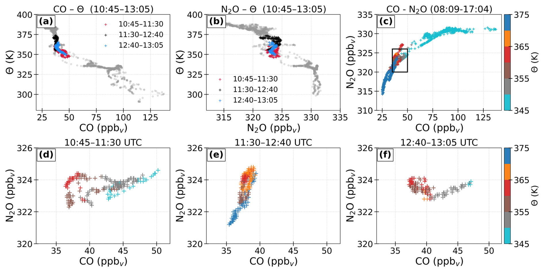
Figure 3 Vertical profiles of (a) CO (in ppbv) and (b) N₂O (in ppbv) with grey circles showing data of the entire flight and color-coded markers indicating the time from 10:45–13:05 UTC. (c–f) Tracer-tracer correlation of the mixing ratios of N₂O and CO for (c) the entire flight and for time periods between (d) 10:45–11:30 UTC, (e) 11:30–12:40 UTC and (f) 12:40–13:05 UTC, color-coded with potential temperature.

In addition, the mixing ratios of both CO and N₂O are well below their tropospheric background values, which is also evident from the CO–N₂O correlation (Fig. 3c). The highlighted period of interest (marked region) is located predominantly within the stratospheric branch and partly within the transition region between troposphere and stratosphere. These regions are characterized by low CO and N₂O mixing ratios, with N₂O values below the well-defined tropospheric background of 331 ppbv during WISE RF05 (see also Kunkel et al., 2019).

Ultimately, irreversible mixing can be inferred from the interrelation of CO, N₂O and potential temperature Θ. Due to the chemical life times, N₂O mixing ratios are almost constant throughout the troposphere, while a chemical sink in the upper stratosphere produces a weak negative vertical gradient. A similar behavior is observed for CO; however, its mixing ratios are less uniform in the troposphere, and the stratospheric gradient above the tropopause is stronger due to stronger chemical removal. Nevertheless, the tracer-tracer relationship remains positive. Consequently, we expect to find a monotonic correlation between CO, N₂O and Θ. As an air mass becomes increasingly stratospheric, the mixing ratios of CO and N₂O decrease, whereas Θ increases. This relationship is apparent in the both the tracer-tracer correlation (Fig. 3c) and the vertical profiles (Fig. 2). Together, they define the expected background relationship among these three quantities. Deviations from this background state can therefore only arise from non-conservative processes. Recent studies highlighted the role of GWs in such situations and the resulting irreversible mixing of trace species (e.g., Kunkel et al., 2019; Lachnitt et al., 2023).

For further analysis, we divide the correlation into three periods: (i) 10:45–11:30 UTC (Fig. 3d), (ii) 11:30–12:40 UTC (Fig. 3e), and (iii) 12:40–13:05 UTC (Fig. 3f). Several interesting features emerge. The first period exhibits two branches connected by a mixing line (around N₂O ∼ 324 ppbv and Θ∼ 359 K). During the second period, only one branch is evident, with Θ values spread across the entire branch. This indicates no clear relationship between Θ and the tracer mixing ratios, although CO and N₂O maintain a compact positive correlation. In the third period, nearly all data points are confined to a small region of correlation space, while potential temperature varies strongly within this region. These features suggest that the air masses were affected by a process that disrupted the relationship between CO, N₂O, and Θ, with irreversible mixing being a likely candidate. Notably, the first and third periods exhibit signatures of recent mixing, coinciding with indications of enhanced turbulence in the ERA5 analysis (Fig. 2b). In contrast, the second period more closely resembles the background CO–N₂O relationship. This may indicate that the air masses sampled during the first and third periods experienced more recent mixing, whereas the air mass sampled during the intervening period had been mixed earlier and had subsequently evolved toward the background tracer relationship.

An analysis of power spectral densities of w, Θ (Fig. 4a, b) and N₂O, CO (Fig. 4c, d) also suggests the presence of small–scale turbulent processes. Overall, the spectra exhibit slopes of $-\mathrm{5}/\mathrm{3}$ which is often seen to support the presence of turbulent motions on the mesoscale and below (e.g., Zhang et al., 2015a; Dörnbrack et al., 2022; Lachnitt et al., 2023). The w spectra show a slope of −3 at smaller wavelengths but transitions to a slope closer to $-\mathrm{5}/\mathrm{3}$ for frequencies below approximately 0.8 Hz, consistent with the findings of Lachnitt et al. (2023). At higher frequencies (shorter wavelengths), the increase in power spectra towards 0.5 Hz may indicate turbulent processes at scales below the synoptic scale. Overall, the w and Θ spectra follow a slope close to $-\mathrm{5}/\mathrm{3}$, consistent with three dimensional isotropic turbulence and suggesting that dynamical processes on or below the mesoscale affect the flow. Moreover, the spectra of N₂O and CO also exhibit slopes close to $-\mathrm{5}/\mathrm{3}$ at intermediate frequencies, corresponding to smaller wavelengths. For frequencies above approximately 10⁻² Hz, the N₂O spectra follow a $-\mathrm{5}/\mathrm{3}$ slope, suggesting that small-scale processes, potentially associated with GWs, contribute to turbulent mixing in the lower stratosphere.

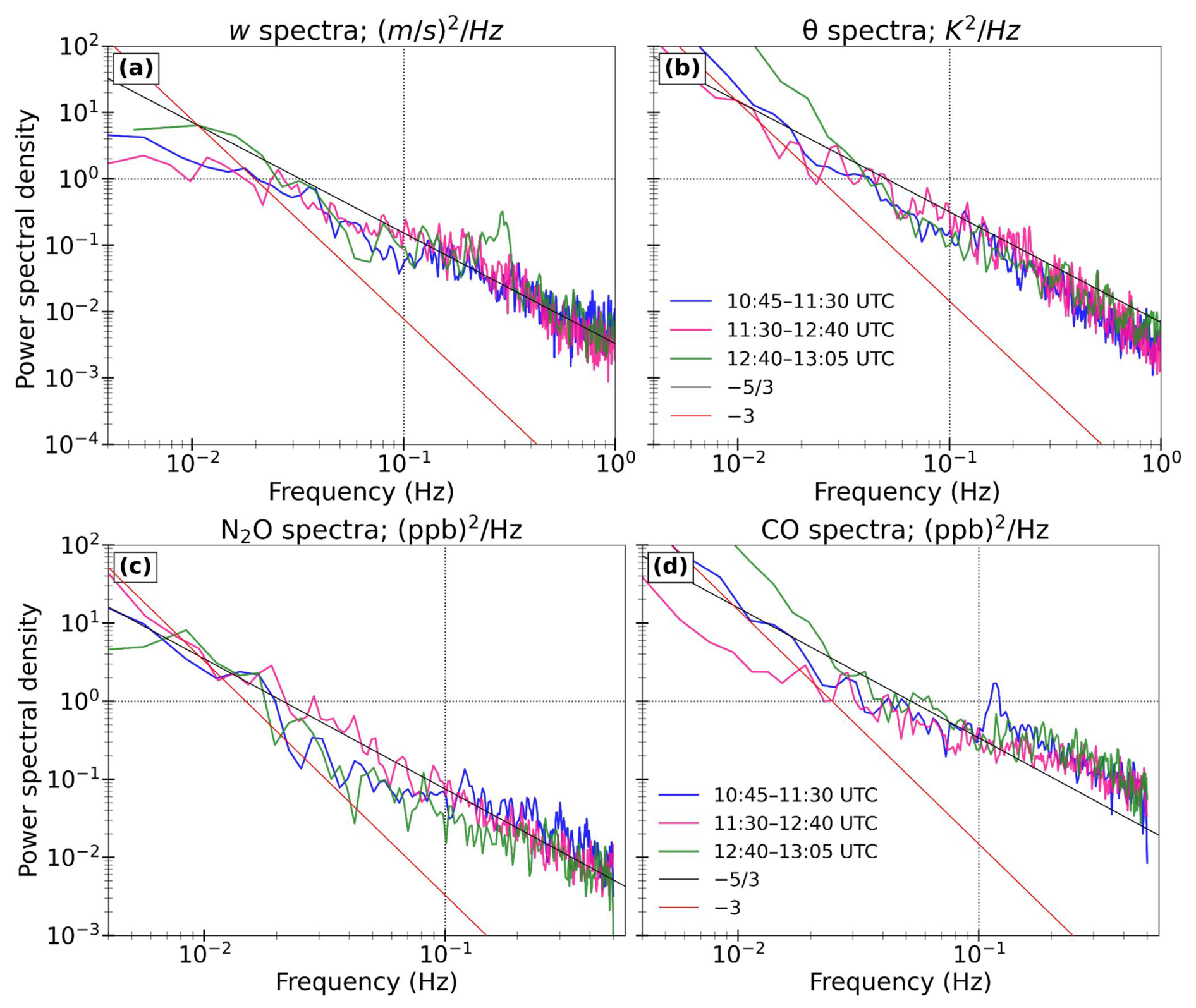
Figure 4 Power spectral densities of (a) measured vertical velocity (in (m s⁻¹)² Hz⁻¹) and (b) observed potential temperature (in K² Hz⁻¹) from BAHAMAS, and of (c) N₂O (in (ppbv)² Hz⁻¹) and (d) CO (in (ppbv)² Hz⁻¹) from UMAQS during WISE RF05 for the time periods 10:45–11:30 UTC (blue lines), 11:30–12:40 UTC (red lines) and 12:40–13:05 UTC (green lines). The orange line indicates the slope of −3 (geostrophic turbulence), the thin black line a slope of $-\mathrm{5}/\mathrm{3}$ (mesoscale turbulence).

The extent to which GW contribute to the mixing of these air masses is difficult to determine based solely on the observations along the flight path. Before we broaden our scope in the analysis to the synoptic scale, we first seek additional observational evidence for the presence of GWs. The high spatial resolution of the in situ measurements allows for resolving mesoscale structures associated with the jet/front system, including regions of low Ri and possible coherent GW phase structures (see Fig. 2). Nevertheless, the temporal resolution of the model output (1 hourly) is too coarse to adequately resolve waves with horizontal wavelengths of approximately 100 km. In contrast, the aircraft observations provide sufficient spatial resolution to identify coherent phase and/or mixing lines in the lower stratosphere, such as those shown in Fig. 3.

To isolate wind perturbations associated with GWs from the background flow, the horizontal wind components (u, v) along the flight track were bandpass filtered using a fourth-order Butterworth filter (Butterworth, 1930). The filter was applied to remove both large–scale trends and high-frequency noise while retaining signals within a 2–10 min period range. The resulting perturbations (u^′, v^′) were then used to construct hodographs and to assess wave properties from the in situ measurements. The resulting perturbation time series are shown in Fig. A4. Note that, due to differences in sampling frequency and noise characteristics in the measurements, the flight data are filtered using a fourth-order Butterworth bandpass filter, whereas the model data are processed using the Helmholtz decomposition approach described in Sect. 2.5, in order to isolate GW related perturbations.

Linear GW theory in a uniform background flow predicts that one vertical wavelength of an inertia GW traces an elliptical perturbation hodograph (as described in Guest et al., 2000; Plougonven et al., 2003; Yoshida et al., 2024) The hodograph rotates anticyclonically for an upward propagating wave and cyclonically for a downward propagating wave. This technique has some limitations under conditions with strong background wind shear and is therefore only applicable to a subset of the wave spectrum, particularly in the low-frequency, long-wavelength limit (for more details see Plougonven et al., 2003). These hodographs are typically derived from vertical profiles at a given time. However, due to the limited number of altitude levels available in our dataset, we instead construct a hodograph from profiles at a single flight altitude using measurements at multiple times (e.g., as in Gomes et al., 2025).

As an example, we use the time series of u^′, v^′ at ∼ 12.5 km flight altitude during the period of enhanced vertical shear and low Richardson number (Fig. 5). The corresponding time series of u, v are shown in Fig. 5a, c (see also Fig. A4). Both periods contain multiple elliptical structures, although only few segments show clear evidence of anticyclonical rotation, highlighted by the red-colored line segments in Fig. 5b, d. A well-defined elliptical pattern is evident in Fig. 5b, indicating the presence of an upward-propagating GW. In contrast, although wave-like oscillations are more prominently observed during 12:45–13:05 UTC (Fig. A4), a similarly coherent elliptical structure is less apparent in Fig. 5d.

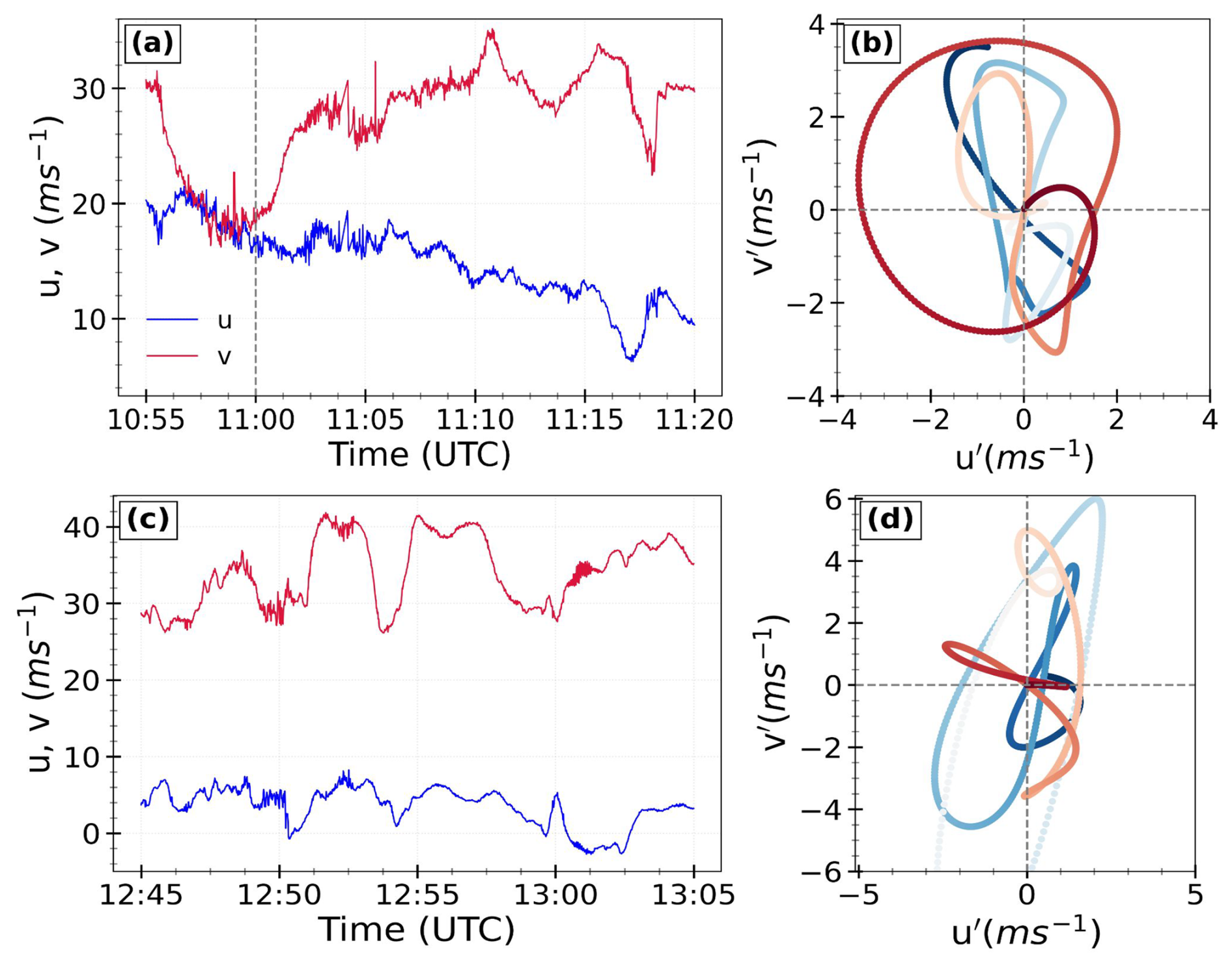
Figure 5 Time series (a, c) of zonal (u, in m s⁻¹; blue) and meridional (v, in m s⁻¹; red) wind component measured during WISE RF05 zoom in for time 10:55–11:20 and 12:45–13:05 UTC. Perturbation hodographs for the corresponding flight period are shown in panels (c) and (d), with trajectories starting in red and ending in blue.

As a first summary, we can conclude that a turbulent region has been crossed during WISE RF05. This region exhibits enhanced vertical shear, low Richardson numbers and signs of tracer mixing. Since there are also signs of GW in the respective time periods, this motivates us to go on with our analysis on how GWs might contribute to this mixing event. For this we will broaden our scope and analyze the larger synoptic situation.

4 Co-occurrence of gravity waves and turbulence in ERA5

In this section, we use ERA5 reanalysis data to investigate potential signatures of GW-induced shear and turbulence. We first examine whether GWs were present over the North Atlantic during the case study period discussed in Sect. 3.3. Subsequently, we explore the relationship between these GWs, vertical wind shear, and turbulence diagnostics in the LMS. Our analysis focuses on the region encompassing the entire flight, defined by 50–72° N and 5–30° W. The analysis domain is outlined in blue in Fig. 1.

4.1 Analysis of gravity waves and vertical shear

We begin by analyzing the horizontal divergence field to identify location and characteristics of potential GW signatures in the LMS. We define the extratropical tropopause based on the dynamical tropopause definition with a potential vorticity value of 3.5 PVU (1 PVU = $\mathrm{1}\times {\mathrm{10}}^{-\mathrm{6}}$ K m² kg⁻¹ s⁻¹).

Figure 6a–c shows the horizontal divergence field at 12.5 km altitude (∼ 200 hPa) between 11:00 and 13:00 UTC. Alternating patterns of divergence and convergence, indicative of gravity wave activity, are evident near the jet streak exit region, with enhanced signatures between 60 and 72° N above the Icelandic highlands along the flight track (Fig. 6a). These GWs are likely generated by the interaction of the baroclinic flow with Iceland's topography. The associated GW signatures persist over the following hours around Iceland (Fig. 6b, c) and are also apparent in the PV field. The horizontal wavelengths of these waves are on the order of a few hundred kilometers, consistent with typical wavelengths of inertia GWs. On the larger scale, however, all time steps exhibit similar divergence patterns, with only slight changes in amplitude and orientation, reflecting a systematic evolution of the wave field.

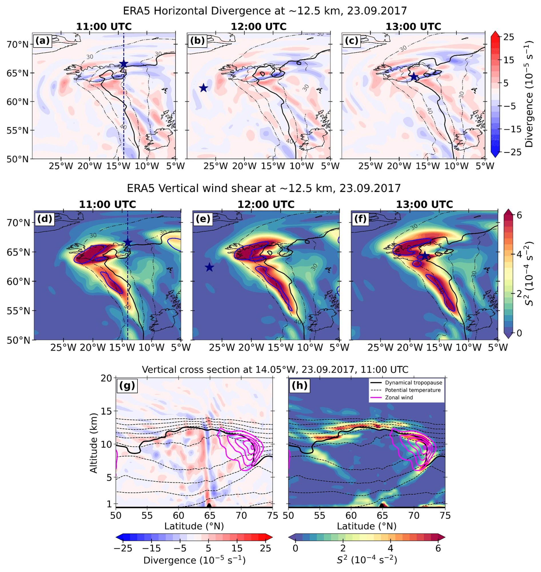
Figure 6 Distribution of horizontal divergence (upper panel) and vertical wind shear (middle panel) at ∼ 12.5 km altitude for ERA5 reanalysis data at 11:00 UTC (a, d), 12:00 UTC (b, e) and 13:00 UTC (c, f). The dashed lines in upper and middle panels represent corresponding horizontal wind speed for values greater than 30 m s⁻¹. The RF05 flight location during the time is marked by blue star. The vertical cross sections of divergence (g) and shear (h) at 14.05° W during 11:00 UTC is shown in lower panel. The solid black line represent the 3.5 PVU as a dynamical tropopause whereas dotted lines in lower panel represent the potential temperature starting from 280 K (bottom) to 380 K (top) with 10 K increments. Magenta contours in (g) and (h) denote zonal wind speed (20, 30, 40, 50) in m s⁻¹ and solid blue lines in middle panel represent Ri=1.

The corresponding vertical cross section of horizontal divergence at 14.05° W, representing the approximate flight location at 11:00 UTC (marked by the dashed line) is shown in Fig. 6g. The GW propagates clearly upward and undergoes changes in wavelength within the LMS. While the GW appears to be rather localized above Iceland in the troposphere, it begins to propagate away from its source region in the stratosphere. At this cross section, the GW signal extends up to an altitude of about 17.5 km. Inspection at later times shows that signal remains persistent, with only minor changes in the wave signatures near 14.05° W (see also Fig. B1). It is further noteworthy that, despite its lower horizontal resolution, ERA5 is able to capture the appearance of GWs in the LMS. This is consistent with findings of previous studies which analyzed GWs in ECMWF products and reanalyses (e.g., Jewtoukoff et al., 2015, and references therein).

Horizontally propagating GWs with large horizontal wavelengths tend to dominate the horizontal derivatives of momentum fluxes, whereas upward-propagating, large-amplitude GWs can transport substantial momentum vertically across the tropopause. This transport can modify the vertical gradients of the wind components across the tropopause, thereby enhancing shear and potentially creating conditions favorable for turbulence development. In the region of the enhanced gravity wave activity, we also find large areas of increased vertical wind shear around 12.5 km altitude between 11:00 and 13:00 UTC. There are clear signs of the enhanced vertical wind shear along the jet-stream south of Iceland. The strongest shear occurs over Iceland in the region of the GW activity (Fig. 6d–f). Additionally, regions of enhanced vertical shear coincide with widespread reduced Ri values (blue lines in Fig. 6d–f), indicating an increased potential for dynamical instability.

Furthermore, the vertical distribution of vertical shear at 14.05° W (Fig. 6h) reveals two distinct regions of enhanced shear. Large shear values are evident in the LMS around the jet stream, roughly around 70° N. In addition, shear maxima occur further south, within the region of GW activity. Since these maxima are located further away from the jet stream, this indicates that other, potentially smaller–scale features contribute to the observed large shear values. Also, there is a clear co-location between large-scale shear and smaller scale shear perturbations (see Fig. B2a) and the GW patterns across the tropopause (Fig. 6d–f). Thus, the vertical alignment of shear perturbations with the GW phase structure remains consistent throughout the tropopause region. Overall, this case exhibits a spatiotemporal co-occurrence of GWs and enhanced vertical wind shear.

While the co-occurrence of GWs and enhanced vertical wind shear suggests a possible link, the extent to which small–scale GWs contribute to shear modification across the tropopause remains to be assessed. One possible explanation is that vertically propagating, large-amplitude GWs with short vertical (and corresponding long horizontal) wavelengths locally modulate the static stability, N², in the LMS (Kunkel et al., 2014; Kaluza et al., 2019; Zhang et al., 2019), which may in turn facilitate the accumulation of vertical shear in this region. This suggests that GWs may partially contribute to, or influence, the enhancement of vertical shear in the lower stratosphere. On the other hand, shear maxima occurring outside regions of GW activity are likely associated with large–scale flow components, including the jet stream and baroclinic disturbance. This motivates a more detailed investigation of the role of small–scale GWs in the development of enhanced vertical shear and, subsequently, their potential contribution to turbulence occurrence.

4.2 Turbulence diagnostics in the LMS

After demonstrating the link between GWs and vertical shear of the total wind field, we move on to a more in-depth analysis of potential turbulence occurrence. Note that turbulence occurrence is assessed with predictors derived from the resolved model quantities. For this purpose, we analyze the AMF and the vertical wind shear perturbations in the region covered by the flight track over the North Atlantic, i.e., between 50–72° N and 5–30° W (see blue box in Fig. 1). We focus on the LMS and further restrict our analysis to regions with gradient Richardson numbers between 0 and 1. The shear perturbations, $S^{{\mathrm{2}}^{\prime }}$, show how much shear is related to the small–scale wind perturbations, whereas the AMF is used to quantify momentum transport associated with GWs. Regions of GW-induced instability and turbulence are expected to coincide with enhanced momentum-flux divergence associated with GW breaking and dissipation (Fritts and Alexander, 2003). We also note that turbulence is a relatively rare phenomenon under typical atmospheric conditions (Sharman et al., 2012; Dörnbrack et al., 2022), and only a limited number of data points are therefore expected during episodes of potential turbulence in the LMS.

With this knowledge, we create two-dimensional probability density distributions of AMF and vertical shear perturbations in the LMS for $\mathrm{0}\le Ri\le \mathrm{1}$ (Fig. 7). The majority of points exhibits relatively low vertical shear values, as indicated by the distribution and color code in the figure. However, regions with the larger vertical shear values ($>\mathrm{3}\times {\mathrm{10}}^{-\mathrm{4}}{\mathrm{s}}^{-\mathrm{2}}$) exhibit also a larger AMF. This suggests a positive correlation between $S^{{\mathrm{2}}^{\prime }}$ and AMF in the LMS and indicates that small–scale processes may contribute to conditions favorable for turbulence occurrence. This behavior is persistent and is especially evident during time periods of interest of our analysis (see Fig. 7a, b for 11:00 and 13:00 UTC). Minor changes in the probability density distributions are apparent and are most likely related to the evolving flow situation. However, the distributions show remarkable similarities to those reported from idealized baroclinic wave experiments (Umbarkar and Kunkel, 2025). We therefore interpret the co-occurrences of enhanced vertical shear perturbations and AMF as evidence that small–scale dynamics, and especially GWs, contribute to the generation of turbulence-favorable conditions. The fact that this relationship is also evident in the idealized experiments further suggests that this is behavior may represent a more general characteristic of baroclinic waves rather than being unique to the present case study.

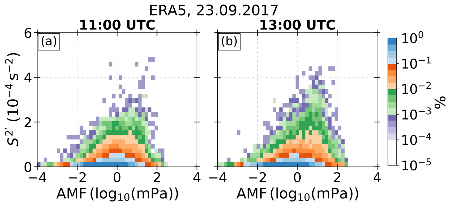
Figure 7 Relative occurrence frequency distribution of absolute momentum flux due to GWs-vertical shear perturbations pair in the LMS for $\mathrm{0}\le Ri\le \mathrm{1}$ for ERA5 reanalysis data at 11:00 UTC (a) and 13:00 UTC (b). Normalized counts of PDF distribution is shown. Logarithmic occurrence frequency color scale is applied.

4.3 Are these GWs responsible for CAT occurrence?

In a next step, we turn to the relationship between GWs and CAT. One previously suggested consequence of dynamical instability is that associated inertia GWs may generate CAT when they break (Knox, 1997). In light of this, Thompson and Schultz (2021) showed that the emission of inertia GWs, following the release of dynamic instability, instigate light–moderate occurrences of CAT around the unstable region using idealized model simulations. We follow this line of thought and use the turbulence indices, TI1 and TI2, to identify regions of potential CAT occurrence in our region of interest in the LMS over the North Atlantic (Fig. 8). In contrast to the shear analysis in the previous sections, CAT develops more sporadically, forming localized pockets. Sharman et al. (2006) suggested that these smaller scale turbulent regions persist for a few minutes around the periphery of the unstable regions. We see similar patterns in our case study. It is noteworthy that the turbulence indices remain low in the region of low gradient Richardson numbers south of Iceland, but reach their largest values over Iceland, where Ri is also small. The TI2 values are generally higher over Iceland than the TI1, which is related to the CVG term in TI2. Together with the fact that the CAT indices are largest in the regions of GW activity, this suggests that GWs play a crucial role in the turbulence formation, despite the limitation of hourly temporal resolution of the ERA5 reanalysis data. Overall, the results support a picture in which upward-propagating GWs modify the flow across the tropopause region, enhance vertical shear, and contribute to the development of dynamical instability and subsequent CAT occurrence.

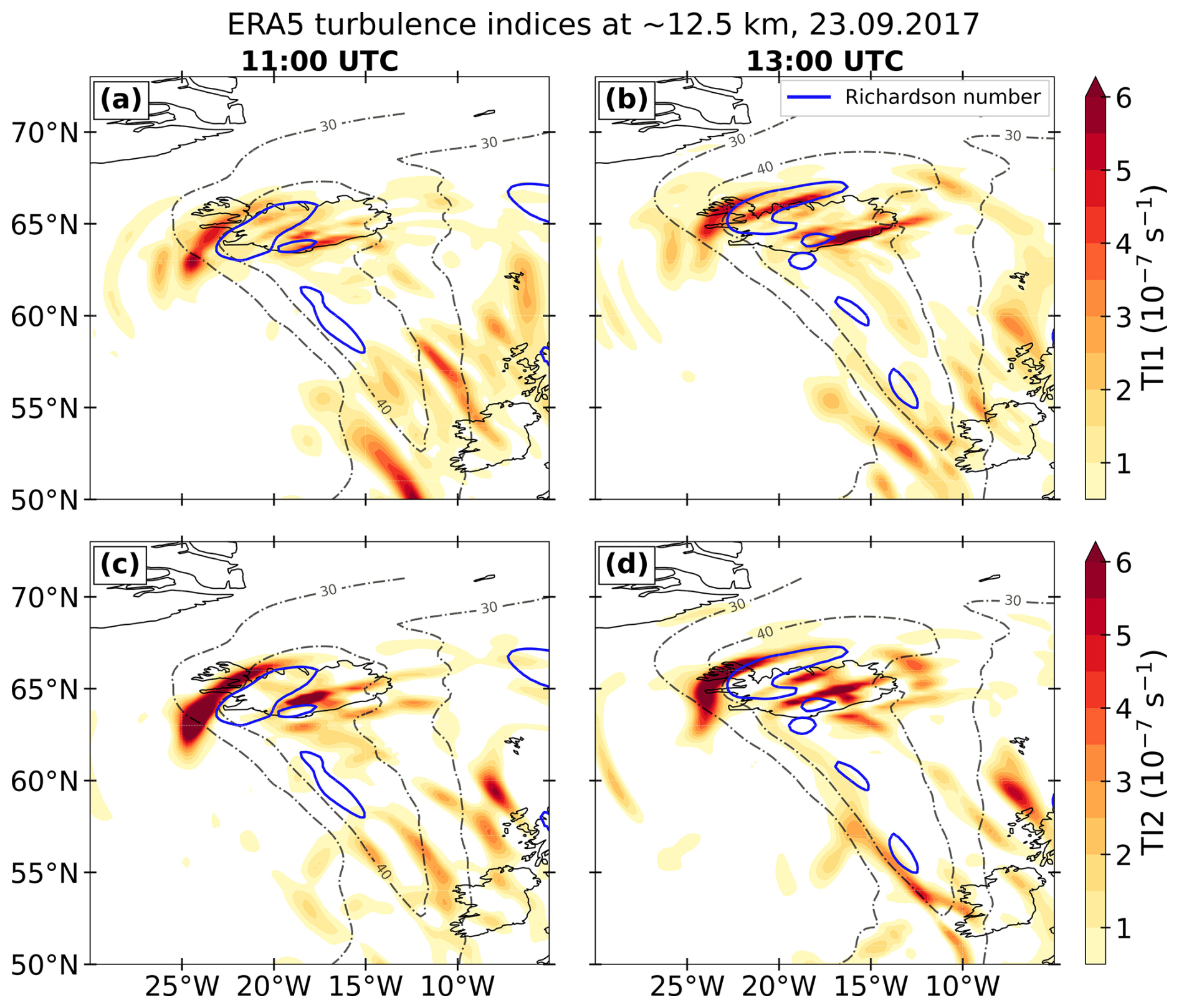
Figure 8 Distribution of turbulent indices TI1 (a, b) and TI2 (c, d) at ∼ 12.5 km altitude for ERA5 reanalysis data at 11:00 and 13:00 UTC. The dashed black lines presents the horizontal wind speed > 30 m s⁻¹ and blue contours denote Ri≤1.

We calculate the TI1 and TI2 as proxies for CAT from zonal and meridional wind perturbations (u^′, v^′). Since we find several regions where CAT develops simultaneously across the tropopause, we use these indices to quantify the intensity of the CAT events based on the ERA5 data. For this purpose, we categorize the CAT values into intensity levels as given in Lee et al. (2019, 2022). Light-to-moderate CAT intensity is defined by the 95th percentile of the distribution of each index within the LMS. In our case, we determine the corresponding threshold values for TI1 and TI2 to $\mathrm{1.4}\times {\mathrm{10}}^{-\mathrm{7}}$ and $\mathrm{1.5}\times {\mathrm{10}}^{-\mathrm{7}}{\mathrm{s}}^{-\mathrm{1}}$, respectively (see also Appendix C and Fig. C1).

Collating all turbulence occurrence throughout the simulation, we find that most occurrences fall into this light–moderate category, but some occurrences of moderate intensity are also apparent (Fig. C1a). In contrast, the moderate to greater intensity CAT events are more prominent in the positive tail of the TI2 distribution than in the TI1 distribution (Fig. C1b). Compared to TI1, TI2 exhibits more frequent occurrences of moderate and greater than moderate CAT events (see Fig. C1b). This difference can likely be attributed to the additional convergence term in TI2, which may further indicate that GWs play an important role in the formation of strong CAT events.

Similar to the analysis of the vertical shear perturbations, we finally examine the relationship between the CAT indices and the AMF. Figure 9 shows the two-dimensional probability density distributions of TI1 and TI2 versus AMF at two time steps for data points in the LMS over the North Atlantic domain. The overall shape of the distributions is quite similar to the distribution for the vertical wind shear perturbations. In both cases, the distributions are tilted toward higher CAT index values and larger AMF, with only minor changes in time (compare panels a and b as well as c and d in Fig. 9). As before, enhanced TI2 values occur more frequently than enhanced TI1 values. Based on these distributions, we suggest that small-scale dynamics, particularly GWs, not only enhance shear, which is a necessary, but not sufficient, condition for turbulence, but also contribute to the occurrence of CAT. Furthermore, these results highlight the important role of the small-scale dynamics in the transport and deposition of momentum across the tropopause, with potential consequences on the distributions of trace species in the UTLS.

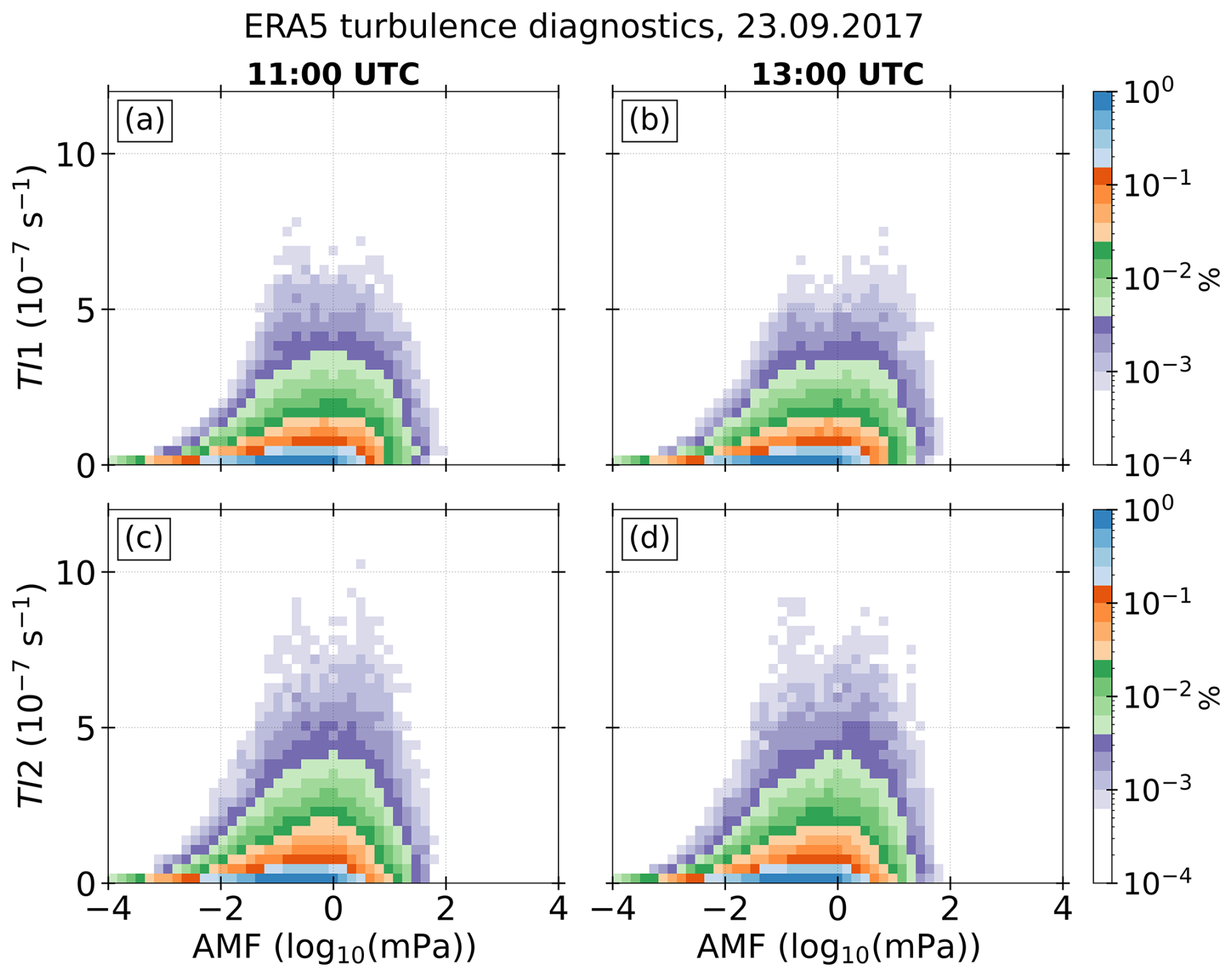
Figure 9 Frequency (%) distribution of absolute momentum flux-turbulent indices TI1 (a, b), TI2 (c, d) in pairs over the LMS for ERA5 reanalysis data at 11:00 and 13:00 UTC. Normalized counts of PDF distribution is shown. Logarithmic occurrence frequency color scale is applied.

In conclusion, the results obtained in Umbarkar and Kunkel (2025) from the idealized cases are also evident in the “real” world in the ERA5 perspective. As of now, the discussion centered around the role of GWs in the occurrence of strong shear in the LMS, and whether potential turbulence occur in the region of the GW-induced shear in ERA5. In the next section, the discussion shifts to a sensitivity analysis with other models.

5 Sensitivity analysis: gravity waves and turbulence occurrences in IFS and ICON

The ERA5 analysis suggests that GWs may contribute to the generation of vertical shear and potential turbulence through dynamical processes. In this section, we investigate how GW signatures change with increasing horizontal resolution and how their occurrence, spatial distribution, and characteristics depend on horizontal grid spacing in the UTLS. From this point onward, we focus on the 11:00 UTC time step, as the analysis at 13:00 UTC leads to the same conclusions regarding the role of GWs in the generation of vertical shear and potential turbulence.

5.1 Analysis of GW, shear and turbulence in the IFS

We first investigate the sensitivity of the results to horizontal resolution using IFS forecasts with a finer spatial resolution than ERA5. At synoptic scales, the flow evolution closely resembles that derived from ERA5 and discussed in Sect. 4.1. However, slight deviations become apparent at the mesoscale as well as in the location of GW structures (Fig. 10). These similarities and differences are illustrated in Fig. 10a, where the IFS resolves finer-scale divergence structures indicative of GW activity over Iceland. In particular, the northwestern sector exhibits more pronounced small–scale features with moderate amplitudes than in ERA5. The corresponding vertical distribution at 14.05° W reveals a GW packet propagating upward into the lower stratosphere, with a relatively large vertical wavelength (∼ 2–3 km) and short horizontal wavelength (∼ 100 km) (Fig. 10c). As expected, the IFS resolves finer-scale wave structures than ERA5 (see also Fig. 6g), indicating that the horizontal characteristics of GWs are strongly dependent on model resolution. This dependence arises not only from the changed grid spacing but also to the representation of orography, as higher horizontal resolution better resolves terrain features and can therefore generate smaller scale orographic GWs. Overall, these results suggest that horizontal resolution strongly influences the representation, spatial structure, and amplitude of resolved GW fluctuations in both reanalyses and forecasts.

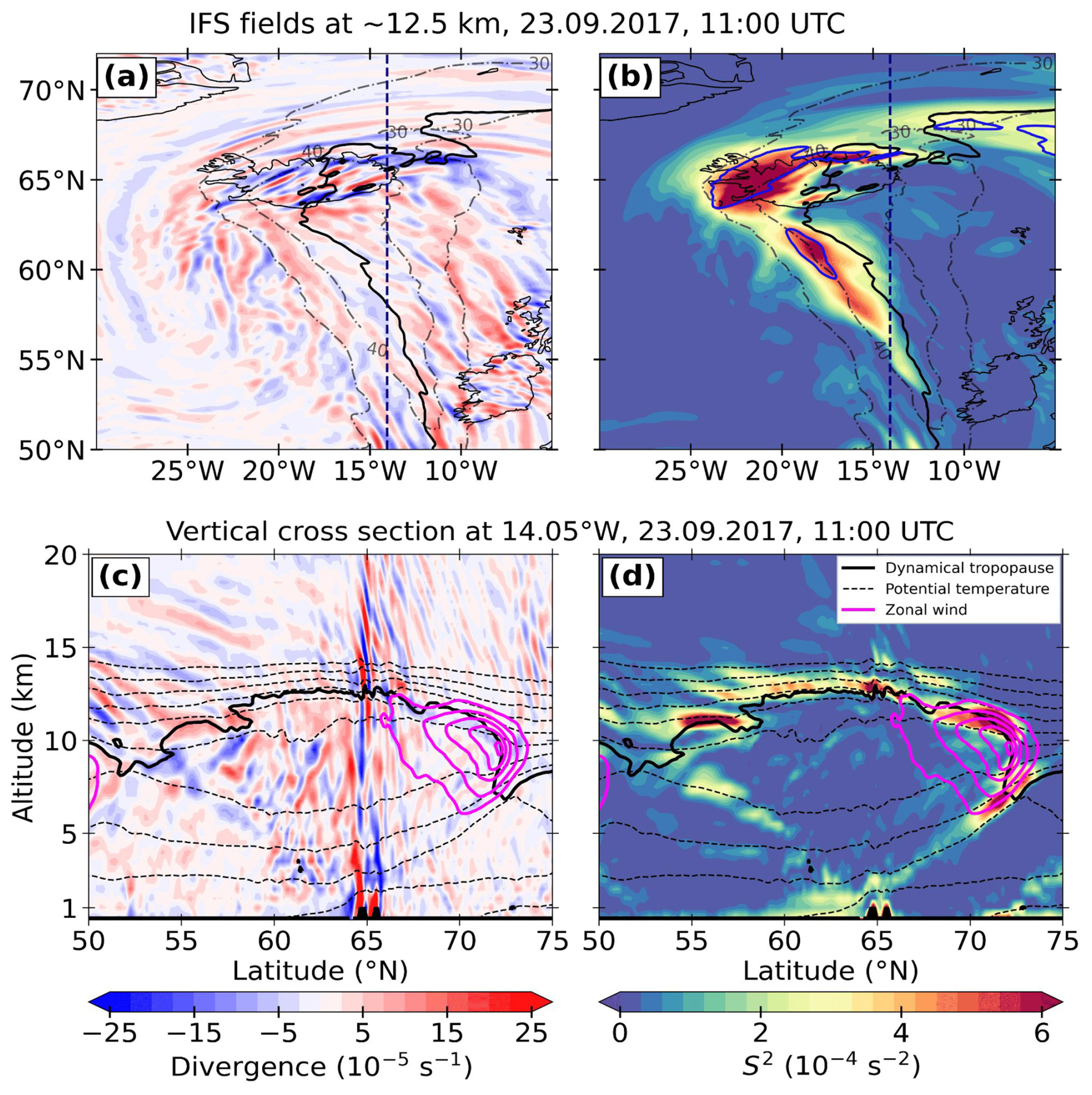
Figure 10 Distribution of horizontal divergence (a) and vertical wind shear (b) at ∼ 12.5 km altitude for IFS data at 11:00 UTC. The dashed lines in upper and middle panels represent corresponding horizontal wind speed for values greater than 30 m s⁻¹. The RF05 flight location during the time shown by blue star. The vertical cross sections of divergence (c) and shear (d) at 14.05° W during 11:00 UTC is shown in bottom panel. The solid black line represent the 3.5 PVU as a dynamical tropopause whereas dotted lines in lower panel represent the potential temperature starting from 280 K (bottom) to 380 K (top) with 10 K increments. Magenta contours in (g) and (h) denote zonal wind speed (20, 30, 40, 50) in m s⁻¹ and solid blue lines in (c) represent the Ri=1.

Further analysis of the vertical shear (Fig. 10b) at the same altitude reveals enhanced shear values around 60–65° N over the Iceland, especially in the proximity of the observed GWs. The large vertical shear values are accompanied by low Richardson numbers, especially over Iceland (blue line in Fig. 10b indicates regions with Ri≤1). This pattern resembles the situation described in ERA5, with a co-occurrence of GWs, enhanced shear and low Ri over Iceland. Farther south, we also identify a region of enhanced shear and low Ri values but clear signatures of GWs. The potential turbulence occurrence in this region is therefore more likely associated with the large–scale flow related to the jet stream. Overall, the IFS exhibits similar patterns of vertical shear, GW activity, and turbulence-favorable regions as ERA5. However, the spatial scales of these features are notably smaller in the vicinity of the ridge. In addition, the IFS shows a clearer spatial correspondence between enhanced shear and GW signatures than ERA5.

Figure 11 Same as Fig. 7 but for IFS at 11:00 UTC.

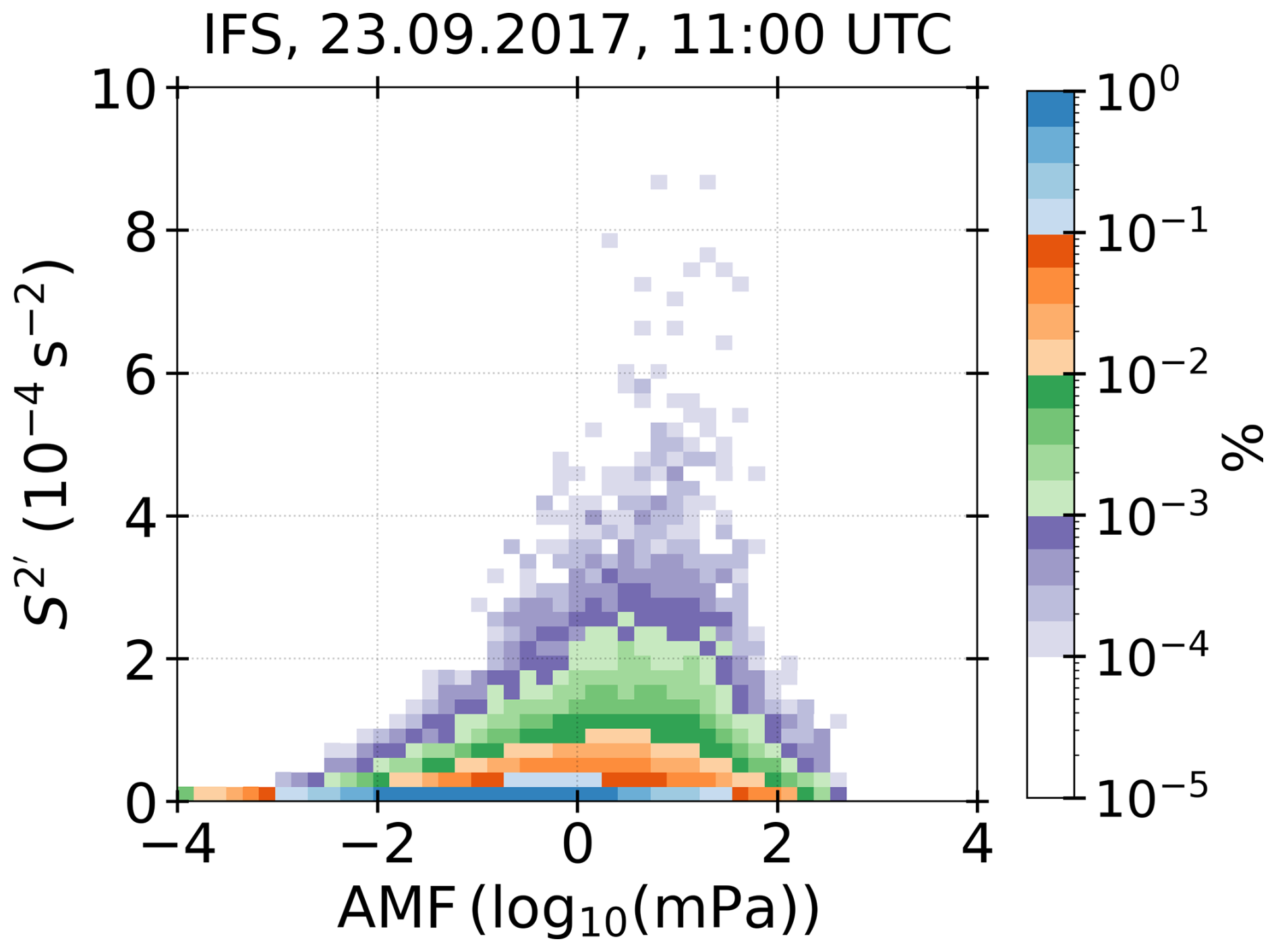
Next, we investigate the perturbation quantities in more detail, starting with the occurrence frequency distribution of AMF and vertical shear perturbations for Richardson numbers between 0 and 1 (Fig. 11). Since IFS resolves the vertical shear similarly to ERA5 and exhibits comparable patterns of GWs activity and S², it is not surprising that the positive correlation between AMF and $S^{{\mathrm{2}}^{\prime }}$ in the LMS remains evident. The most notable difference is that larger absolute values of shear perturbations are present in the IFS data, and the occurrence of strong shear perturbations is increased compared to ERA5 (see Fig. 7). The AMF also shows slightly larger values, indicating somewhat enhanced GW activity. Thus, the higher-resolution data further support and strengthen our hypothesis that small–scale dynamics are a vital contributor to the occurrence of enhanced shear and subsequently to conditions favorable for turbulence formation in the LMS.

With the apparently stronger shear and GW activity in the IFS forecast compared to ERA5, the next question is whether this also results in an increased occurrence of potential turbulence. To address this, we analyze the occurrences of TI1 and TI2, starting with their horizontal distributions (Fig. 12). As in ERA5 (see Fig. 8), the overall spatial structure is similar, but the regions of enhanced TI1 and TI2 are more localized in the IFS. The two indices show only minor differences in their spatial distribution, with TI2 exhibiting slightly larger values. Interestingly, regions of low Richardson number, indicated by the blue contour, show little overlap with regions of enhanced turbulence indices.

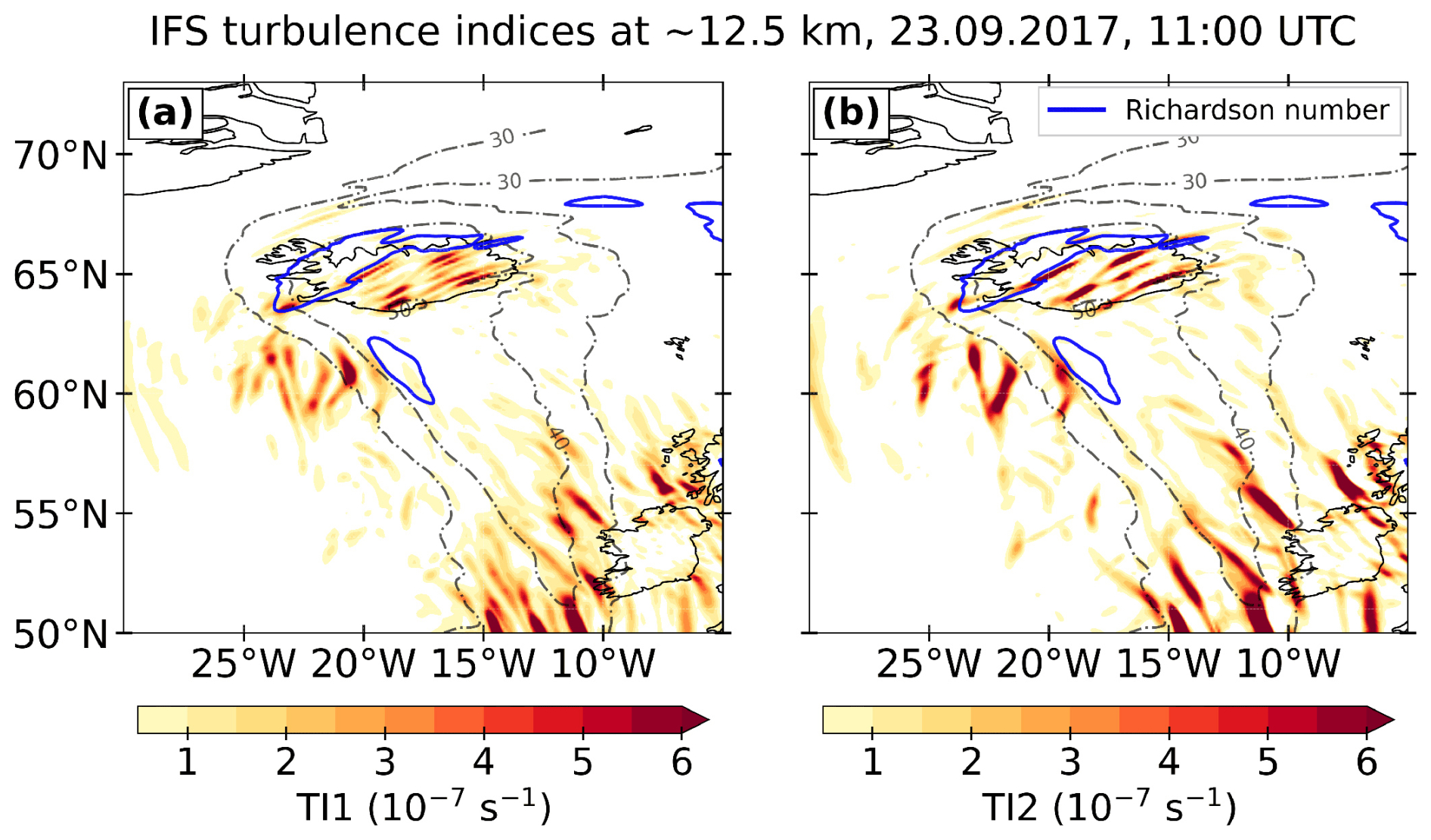
Figure 12 Distribution of turbulent indices TI1 (a) and TI2 (b) at ∼ 12.5 km altitude for IFS data. The dashed black lines presents the horizontal wind speed $>\mathrm{30}\mathrm{m}{\mathrm{s}}^{-\mathrm{1}}$ and blue contours denote Ri=1.

Figure 13 Frequency (%) distribution of absolute momentum flux-turbulent indices TI1 (a), TI2 (b) in pairs over the LMS for IFS data. Normalized counts of PDF distribution is shown. Logarithmic occurrence frequency color scale is applied.

As before, we determine the threshold value for light moderate CAT based on the 95th percentile criterion. The resulting threshold values for TI1 and TI2 are then $\mathrm{2.1}\times {\mathrm{10}}^{-\mathrm{7}}{\mathrm{s}}^{-\mathrm{1}}$ and $\mathrm{2.45}\times {\mathrm{10}}^{-\mathrm{7}}{\mathrm{s}}^{-\mathrm{1}}$, respectively (Fig. C1). Both values are remarkably higher than the corresponding ERA5 threshold values, further highlighting that the IFS resolves clearer signatures of potential turbulence occurrence. This behavior is also evident across the entire LMS, as shown by the two-dimensional occurrence frequency distributions of TI1-AMF and TI2-AMF pairs (Fig. 13). Compared to ERA5, the distributions exhibit slightly higher maximum values of TI1 and TI2. More importantly, they show a larger frequency of high turbulence-index values, suggesting an increased occurrence of potential turbulence in the LMS. Both distributions are skewed toward high AMF and high turbulence indices, further supporting the link between turbulence occurrence and GW activity.

So far, this section has focused on the role of GWs in generating strong shear in the LMS and on whether clear-air turbulence occurs within regions of GW-induced shear in ECMWF datasets, which employ a hydrostatic dynamical core together with semi-implicit and semi-Lagrangian numerical schemes. We now investigate whether these findings also hold in ICON simulations of the same case. This provides a unique opportunity to examine the event across three model domains (with and without convective parameterization) and to relate the results to our previous idealized ICON simulations (Umbarkar and Kunkel, 2025).

5.2 Analysis of GW, shear and turbulence in the ICON model

In this section, we not only compare the ICON model, which employs a non-hydrostatic dynamical core, with the hydrostatic ECMWF models, but also investigate the impact of horizontal resolution within the ICON framework. To this end, we analyze simulations ranging from the global configuration with an effective horizontal grid spacing of 13 km to a nested configuration with an effective grid spacing of 3.3 km. Further details on the model setup and the physical parameterization schemes used in these simulations are provided in Sect. 2.4.

We begin by examining the horizontal divergence at 12.5 km altitude (Fig. 14). Overall, the structure closely resembles that of the ECMWF models (reanalysis and forecast). Pronounced GW activity over the northeastern Icelandic highlands is evident in all ICON domains (Fig. 14a–c), with enhanced wave signatures between 60 and 72° N, particularly over and east of Iceland along the flight track. The ICON simulation with Δx≈3.3 km captures GW activity throughout the analysis domain, including moderate wave activity in the northwestern sector (Fig. 14c). The GWs in this instance generally exhibit larger-amplitudes, but are spatially more confined.

Notably, the ICON simulation with Δx≈6.5 km reveals prominent upward-propagating GWs with relatively small amplitudes that closely resemble those resolved by the IFS but are not clearly captured in ERA5 (see also Fig. B3). Likewise, the Δx≈13 km simulation exhibits a vertical structure similar to that of the IFS, with a slightly shorter vertical wavelength of approximately 3 km and wave signatures extending up to about 17.5 km altitude (Fig. B3a). In contrast, the finer-resolution simulation (Fig. B3c) resolves larger-amplitude waves with longer vertical wavelengths that propagate upward beyond approximately 19 km altitude. It should be noted that the shallow convection scheme employed in the nested domains (Δx≈6.5 km and Δx≈3.3 km) may contribute to the emergence of additional small–scale wave signatures. All three domain clearly exhibit a more pronounced GW signatures as the horizontal resolution increases, with slight differences evident in both amplitude and spatial structure of the GWs. This highlights that the representation and occurrence of GWs, as well as associated small–scale features, depend substantially on the model grid spacing and convection processes implemented in the respective domains.

The corresponding horizontal distribution of vertical shear (Fig. 14d–f) shows the maximum shear values north-east from the strongest GW signatures, north of 65° N and east of 14° W. The three domains show similar structures, in particular, the region of enhanced shear south of Iceland is weaker in ICON than in the ECMWF models. The ICON simulation with the finest grid spacing shows the highest shear values, and the shear becomes more localized with pronounced banded structures in regions of strong divergent signals. This suggests a close relationship between horizontal divergence and vertical shear in the tropopause region and in the lower stratosphere (see also Fig. B3d–f). The enhanced small–scale divergence in the higher-resolution simulations may partly arise from differences in the representation of convective processes and associated gravity wave sources. Moreover, this overall behavior indicates that both horizontal and temporal resolution substantially influence the amplitude and representation of GW-related fluctuations in the forecast data, consistent with the findings presented in Sect. 5.1. These results highlight the need for sufficient horizontal resolution to accurately represent GWs and small–scale processes.

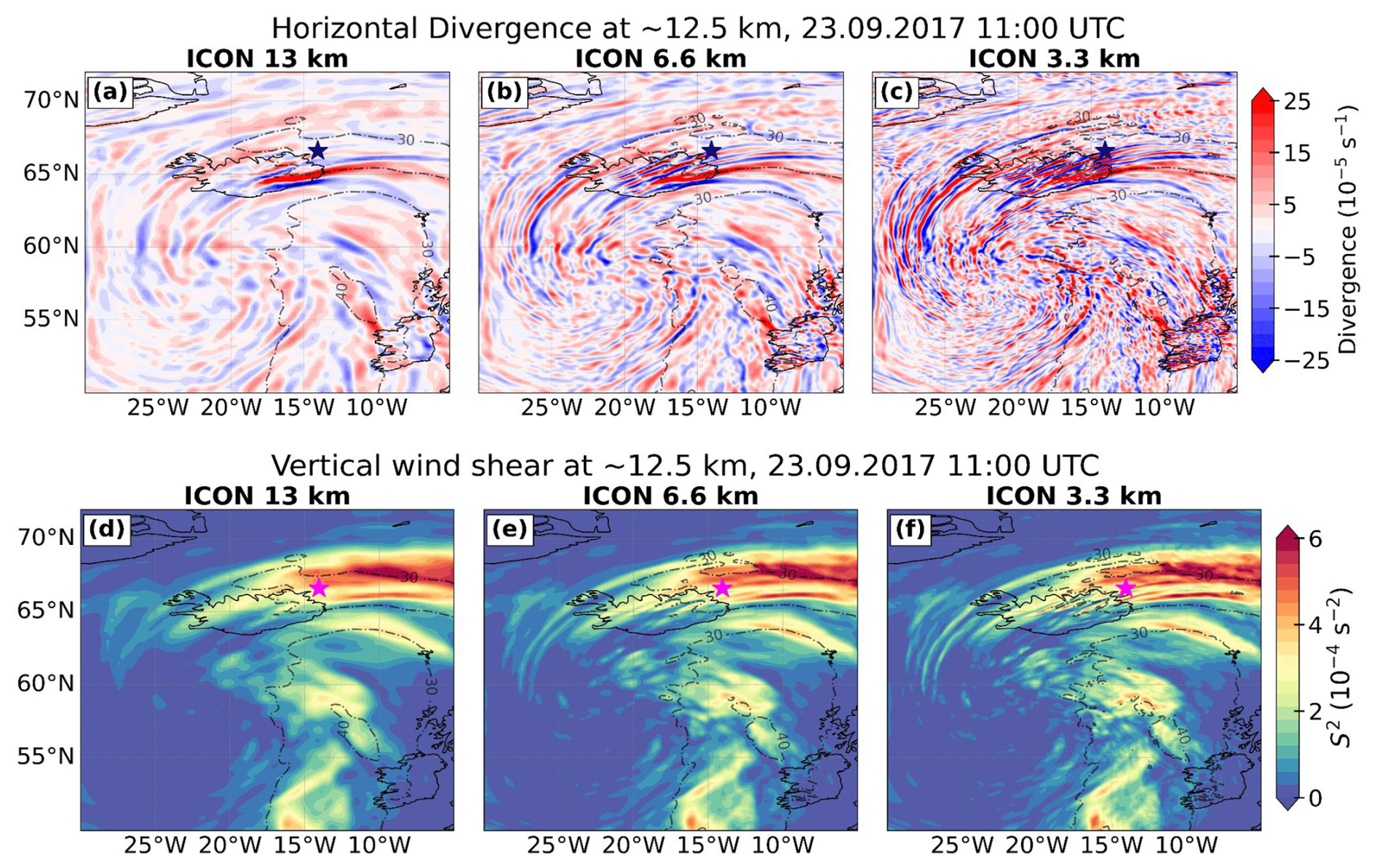
Figure 14 Distribution of horizontal divergence (upper panel) and vertical wind shear (lower panel) at ∼ 12.5 km altitude for ICON 13, 6.5 and 3.3 km resolution nested simulations overlaid with flight location at 11:00 UTC marked with star. The dashed line represent corresponding horizontal wind speed for values greater than 30 m s⁻¹.

Diagnostics of potential turbulence and CAT in the LMS

Next, we investigate the previously identified relationship between momentum flux and shear perturbations in the context of potential turbulence occurrence within the LMS. For this, both AMF and $S^{{\mathrm{2}}^{\prime }}$ quantities are masked to regions in the LMS where potential turbulence (i.e., $\mathrm{0}\le Ri\le \mathrm{1}$) may occur. A closer examination reveals that the AMF generally attains larger values than in ERA5 and IFS, while the shear perturbations also reach substantially higher values than in the ECMWF models (see Fig. 15). It becomes also clear that the maximum shear perturbations increase substantially with increasing horizontal resolution. The most pronounced change in the distribution occurs between the Δx≈13 km and the Δx≈6.5 km simulations, whereas the differences between the 6.5 and 3.3 km simulations are comparatively smaller. Nevertheless, the ICON simulations consistently show that finer horizontal grid spacing is associated with both stronger shear perturbations and enhanced GW activity, as reflected by the larger AMF values.

Figure 15 Relative occurrence frequency distribution of absolute momentum flux due to GWs-vertical shear perturbations pair in the LMS for $\mathrm{0}\le Ri\le \mathrm{1}$ for ICON 13, 6.5 and 3.3 km resolution nested simulations at 11:00 UTC. Normalized counts of PDFs distribution is shown. Logarithmic occurrence frequency color scale is applied.

The similarity of the distributions in the two higher-resolution simulations is particularly noteworthy, since they differ in their representation of the convection. In the Δx≈3.3 km simulation, convection is permitted, whereas it remains parameterized in the Δx≈6.5 km simulation. Nevertheless, the relationship between AMF and $S^{{\mathrm{2}}^{\prime }}$ exhibits an almost identical pattern during potential turbulent episodes (see red colors shading in Fig. 15b, c). Thus, while finer resolution provides a more detailed representation of the GW field, the positive association between momentum flux and enhanced shear remains robust across all simulations. This behavior is consistent with the results presented in Sect. 5.1 and with idealized studies showing that GW-induced perturbations enhance vertical shear, thereby preconditioning the flow for shear-driven instabilities and subsequent potential turbulence generation.

Up to this point, the analyses of vertical shear, shear perturbations, and absolute GW momentum flux have provided evidence for conditions favorable to turbulence occurrence. However, it remains possible that the identified regions of enhanced shear and small–scale variability are primarily associated with the synoptic-scale flow rather than directly linked to clear-air turbulence. While the preceding interpretation relies on previous studies, this issue can be addressed more directly by examining the relationship between the CAT indices and AMF.

Again, we briefly examine the turbulence indices TI1 and TI2 calculated on the three ICON domains to assess potential differences between the ICON domains and between ICON and ERA5. For both indices, the transition from the coarsest to the finest ICON resolution leads to substantial changes. Although the overall spatial patterns of TI1 and TI2 remain similar, their magnitude and mesoscale structure differ considerably. In particular, banded regions of enhanced TI1 and TI2 develop over the North Atlantic and Iceland. These bands become more pronounced and exhibit larger index values as the horizontal resolution increases (Fig. 16). Overall, the large–scale distribution of potential turbulence is similar in the ICON, ERA5, and IFS datasets, whereas the differences become increasingly apparent at the mesoscale. The higher-resolution simulations resolve more localized regions of enhanced turbulence indices, which also attain larger values. This likely reflects the broader range of the GW spectrum resolved at finer horizontal resolution. Consequently, larger parts of the domain exhibit conditions favorable for potential turbulence occurrence. This is expected and is also reflected in the relative occurrence frequency of TI1 and TI2 (Fig. 17). The largest TI1 and TI2 values occur in the highest-resolution ICON simulation, indicating that stronger signatures of potential CAT are resolved in this domain. It is particularly interesting that at smaller TI1 and TI2 values, the histograms for the two finer resolved ICON simulations exhibit nearly identical relative frequencies, whereas they differ substantially at larger values corresponding to stronger turbulence conditions. Additionally, the ICON and IFS simulations show similar relative frequencies of TI1 and TI2, especially more intense turbulence occurrence for the moderate and moderate-or-greater CAT category (see also Appendix C).

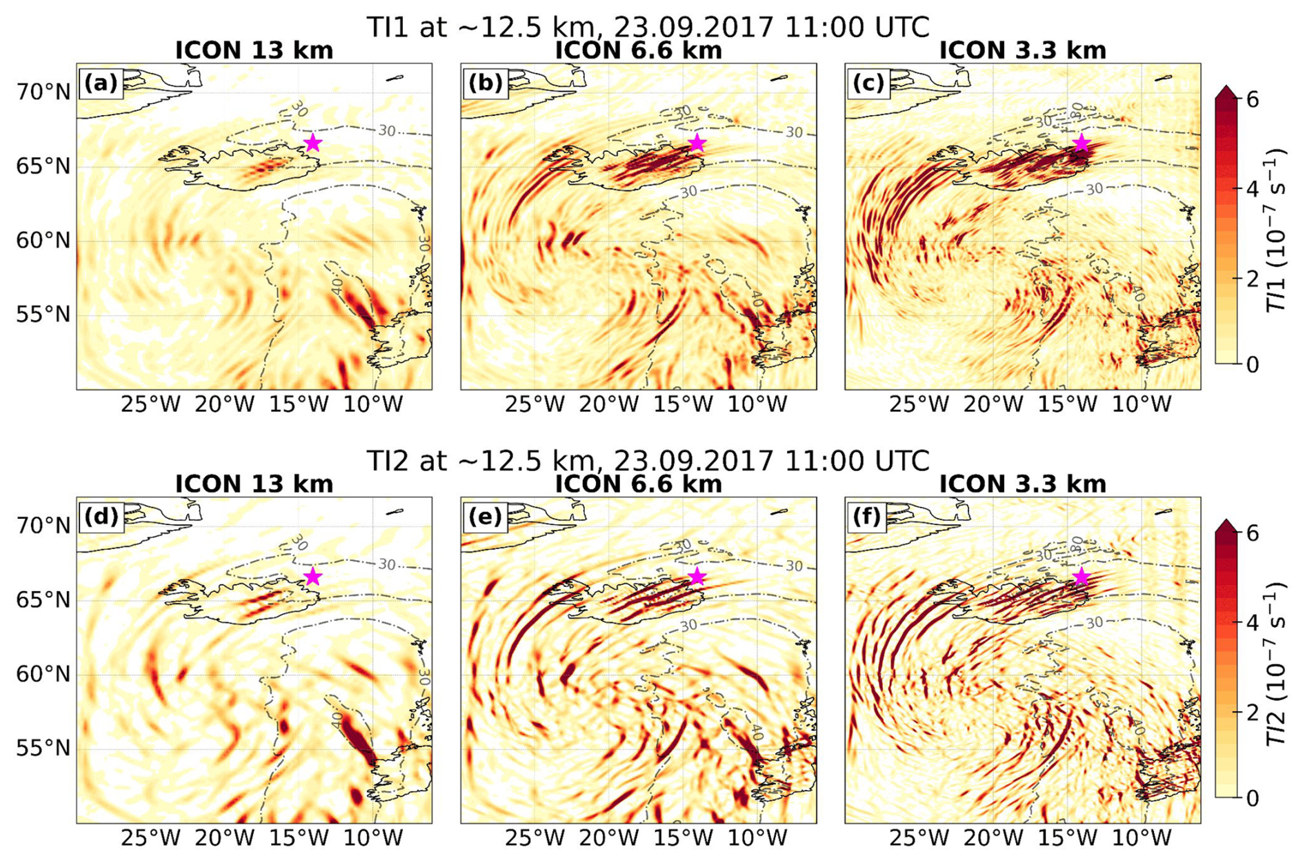
Figure 16 Distribution of turbulence indices TI1 (a–c) and TI2 (d–f) at ∼ 12.5 km altitude for ICON 13, 6.5 and 3.3 km resolution nested simulations. The dashed line represent corresponding horizontal wind speed for values greater than 30 m s⁻¹.

Figure 17 Relative occurrence frequency distribution of (a) TI1 and (b) TI2 for three ICON domains in the LMS. Corresponding to histogram, colored dashed lines indicate threshold retrieved as the 95th percentile over the LMS domain distribution that is considered as threshold for light moderate category. Grey and aqua lines represent the threshold for moderate (7.5–$\mathrm{12}\times {\mathrm{10}}^{-\mathrm{7}}{\mathrm{s}}^{-\mathrm{1}}$) and moderate to greater ($>\mathrm{12}\times {\mathrm{10}}^{-\mathrm{7}}{\mathrm{s}}^{-\mathrm{1}}$) intensity CAT, respectively.

The joint histograms of TI1-AMF and TI2-AMF pairs in the LMS further support the previous findings by showing a positive relationship between turbulence indices and AMF across all horizontal resolutions (Fig. 18). Additionally, both the turbulence indices and the AMF reach larger values as the horizontal grid spacing decreases. One possible explanation for this could be the stronger GWs associated with convective sources in the higher-resolution simulations. Together with the better resolved small–scale dynamical features, this likely contributes to the enhanced shear and larger turbulence indices. These results suggest that vertically propagating GWs, through their contribution to enhanced vertical shear, play an important role not only in the generation of CAT but also in its evolution. More generally, this suggests that improved representation of small–scale structures at higher resolution may lead to more accurate predictions of such CAT events.

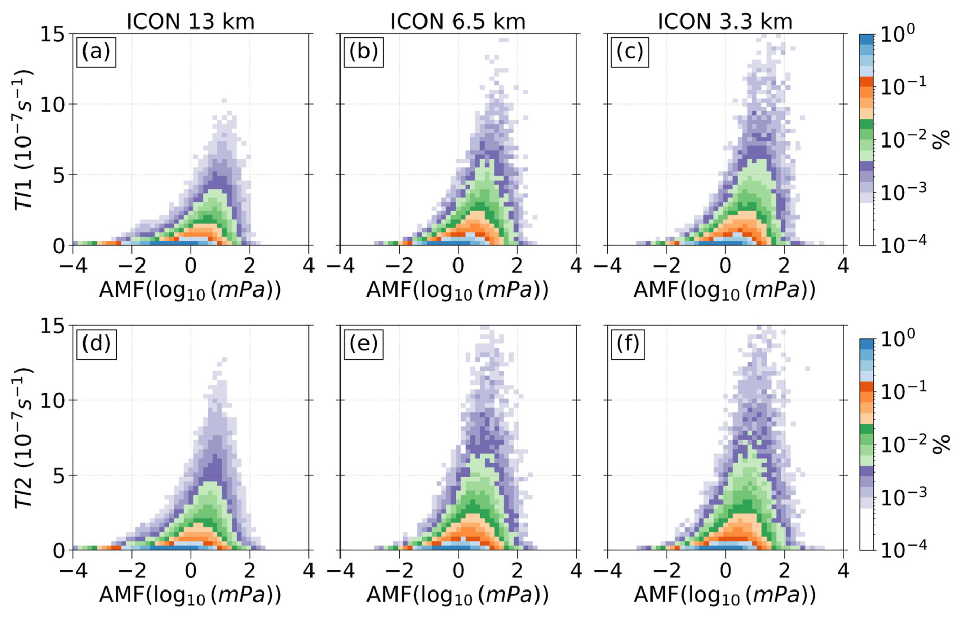
Figure 18 Frequency (%) distribution of absolute momentum flux–turbulent indices TI1 (a–c), TI2 (d–f) in pairs over the LMS for ICON 13, 6.5 and 3.3 km resolution nested simulations at 11:00 UTC. Normalized counts of PDFs distribution is shown. Logarithmic occurrence frequency color scale is applied.

An interesting observation is the more frequent occurrence of positive TI1-AMF and of TI2-AMF relationships in ICON compared with Fig. 15, despite ICON exhibiting weaker and more fragmented shear perturbations in regions of low Ri than ERA5 (Fig. 7) and IFS (Fig. 11). One possible explanation is that enhanced local flow deformation contributes to the turbulence indices and partly offsets the impact of weaker resolved shear, resulting in a higher occurrence of elevated TI1 values within GW-affected regions. Nevertheless, the forecast skill of DEF as a turbulence diagnostic has previously been linked to frontogenesis, enhancement of thermal wind shear (Ellrod and Knapp, 1992), and local GW activity (Kunkel et al., 2014).

Furthermore, results from both the IFS and ICON simulations support the hypothesis that the sensitivity to spatio-temporal resolution primarily arises from horizontally propagating GWs with large horizontal wavelengths, which dominate the horizontal gradients of momentum flux. In contrast, large-amplitude upward-propagating GWs mainly contribute to enhanced vertical wind shear through vertical gradients of the wind components. Together, these effects promote stronger shear, lower Richardson numbers, an increased likelihood of dynamic instability, and consequently higher occurrences of TI1 and TI2.

6 Turbulence diagnostics in a zonal framework

In this section, we turn our attention to a more general feature of the LMS which has been described recently in Kaluza et al. (2021, 2022). We first examine the occurrence of the extratropical TSL (Kaluza et al., 2021) across three available datasets: two ECMWF products and a large domain ICON simulation. Afterwards, we investigate the role of GWs in the formation of the TSL and assess whether turbulence occurs within the TSL region. Here, we consider ICON simulation with Δx≈13 km, as this is the resolution closer to the ECMWF reanalysis and forecast data. This allows us to obtain a consistent comparison of synoptic-scale structures across the extratropical LMS.

We first examine the occurrence of enhanced vertical shear in the extratropics. The TSL has been defined via an exceedance of a defined threshold value of vertical wind shear, i.e., S² ≥ $S_{\mathrm{t}}^{\mathrm{2}}$ where $S_{\mathrm{t}}^{\mathrm{2}}$ = $\mathrm{4}\times {\mathrm{10}}^{-\mathrm{4}}{\mathrm{s}}^{-\mathrm{2}}$ (Kaluza et al., 2021). We apply an analogous method to our case study at an instantaneous time step in our limited area over the North Atlantic. Figure 19a–c shows the relative occurrence frequencies, counted in the zonal direction, of S² exceeding the threshold in the UTLS. In regions of elevated tropopause altitude, enhanced shear occurrences are associated with ridges of baroclinic waves and GW activity (e.g., Kaluza et al., 2021; Kunkel et al., 2019; see also Sect. 4.1). In our case, pronounced shear occurrences are found between 45 and 60° N in ERA5 and IFS, while they are slightly less frequent in ICON. Overall, this further supports the results observed in Sects. 4.2 and 5, where the LMS exhibits enhanced shear occurrence near Iceland associated with elevated GW momentum flux.

Figure 19 Relative occurrence frequency distribution of grid volumes that exhibit (a–c) S² $\ge \mathrm{4}\times {\mathrm{10}}^{-\mathrm{4}}{\mathrm{s}}^{-\mathrm{2}}$, (d–f) TI1 $\ge \mathrm{7.5}\times {\mathrm{10}}^{-\mathrm{7}}{\mathrm{s}}^{-\mathrm{1}}$ and (g–i) TI2 $\ge \mathrm{7.5}\times {\mathrm{10}}^{-\mathrm{7}}{\mathrm{s}}^{-\mathrm{1}}$ over the North Atlantic domain on 23 September 2017, 11:00 UTC for ERA5, IFS, and ICON. Panels (d)–(i) represent regions of moderate-intensity CAT occurrence. The occurrence frequencies are shown with logarithmic frequency contours, displaying the data in bins of sizes Δ y=0.2° and Δ z = 500 m. The zonal-mean dynamical tropopause (3.5 PVU isosurface; black dashed line) and the zonal-mean 380 K isentrope of potential temperature (solid line) are overlaid.

We further explore the relationship to potential turbulence by examining the zonal occurrence frequencies of the CAT indices, i.e., TI1 and TI2 exceeding the threshold for moderate CAT occurrences ($\ge \mathrm{7.5}\times {\mathrm{10}}^{-\mathrm{7}}{\mathrm{s}}^{-\mathrm{1}}$, Fig. 19d–i). The zonally integrated distributions of TI1 show enhanced occurrences within and north of the regions with strong shear (Fig. 19d–f). In ERA5, enhanced occurrence frequencies indicate a relatively large fraction of moderate CAT events within the total number of potential CAT occurrences, particularly around 50° N in the LMS. The IFS rather shows pronounced CAT occurrences between 45 and 60° N (Fig. 19e), with TI2 occurrences being more meridionally spread out (Fig. 19h). In contrast to the similarities between ICON and IFS in Sect. 5, the ICON simulation exhibits slightly lower occurrence frequencies of the CAT indices (Fig. 19f, i). Overall, both TI1 and TI2 exhibit very similar patterns in terms of occurrences in the LMS (compare Fig. 19d–f and g–i). Conversely, regions of enhanced shear without corresponding TI1 occurrences (e.g., near 35 and 70° N in ERA5 and IFS) suggest that shear is more associated with large–scale dynamical features, such as the jet stream, rather than with GW activity. In sum, the turbulence diagnostics reveal turbulence hotspots near typical aircraft cruising altitudes (∼ 10–13.5 km) across the North Atlantic in all datasets, consistent with the altitude range where strong shear layers frequently occur.

The question remains whether GWs contribute to the formation of the extratropical TSL and, consequently, to CAT hotspots. Upward-propagating, short-horizontal-wavelength GWs can carry substantial vertical momentum fluxes. If these waves contribute to CAT generation, momentum-flux deposition would be expected in regions where GW-induced turbulence occurs. The largest AMF magnitudes are concentrated in the upper troposphere and extend into the lower stratosphere (Fig. D1). At first glance, regions of enhanced AMF and strong vertical AMF gradients appear to coincide with areas of elevated shear S² ≥ $S_{\mathrm{t}}^{\mathrm{2}}$ and elevated turbulence potential in the LMS. If GWs indeed play a significant role, one would expect at least a quasi-spatial co-occurrence of enhanced shear, elevated turbulence indices, and increased GW momentum flux.

Figure 20 shows the AMF in regions of enhanced shear and areas prone to moderate-intensity CAT. In the vicinity of strong shear, both ERA5 and IFS exhibit enhanced AMF predominantly above the tropopause, particularly at midlatitudes (Fig. 20a, b). Notably, ERA5 displays a pattern similar to that of IFS, despite its lower horizontal resolution. In contrast, ICON reveals more localized but substantially stronger AMF maxima near regions of enhanced shear (Fig. 20c). These elevated fluxes indicate enhanced GW activity associated with baroclinic disturbances. Regions of pronounced shear largely coincide with areas of enhanced GW activity, supporting the previously identified relationship between GWs and enhanced shear. This spatial overlap further suggests that small–scale processes may contribute significantly to turbulent mixing. These findings further agree with the conclusion of the previous studies of baroclinic life cycles (Kaluza et al., 2019, 2021) and process studies (Kunkel et al., 2019; Umbarkar and Kunkel, 2025).

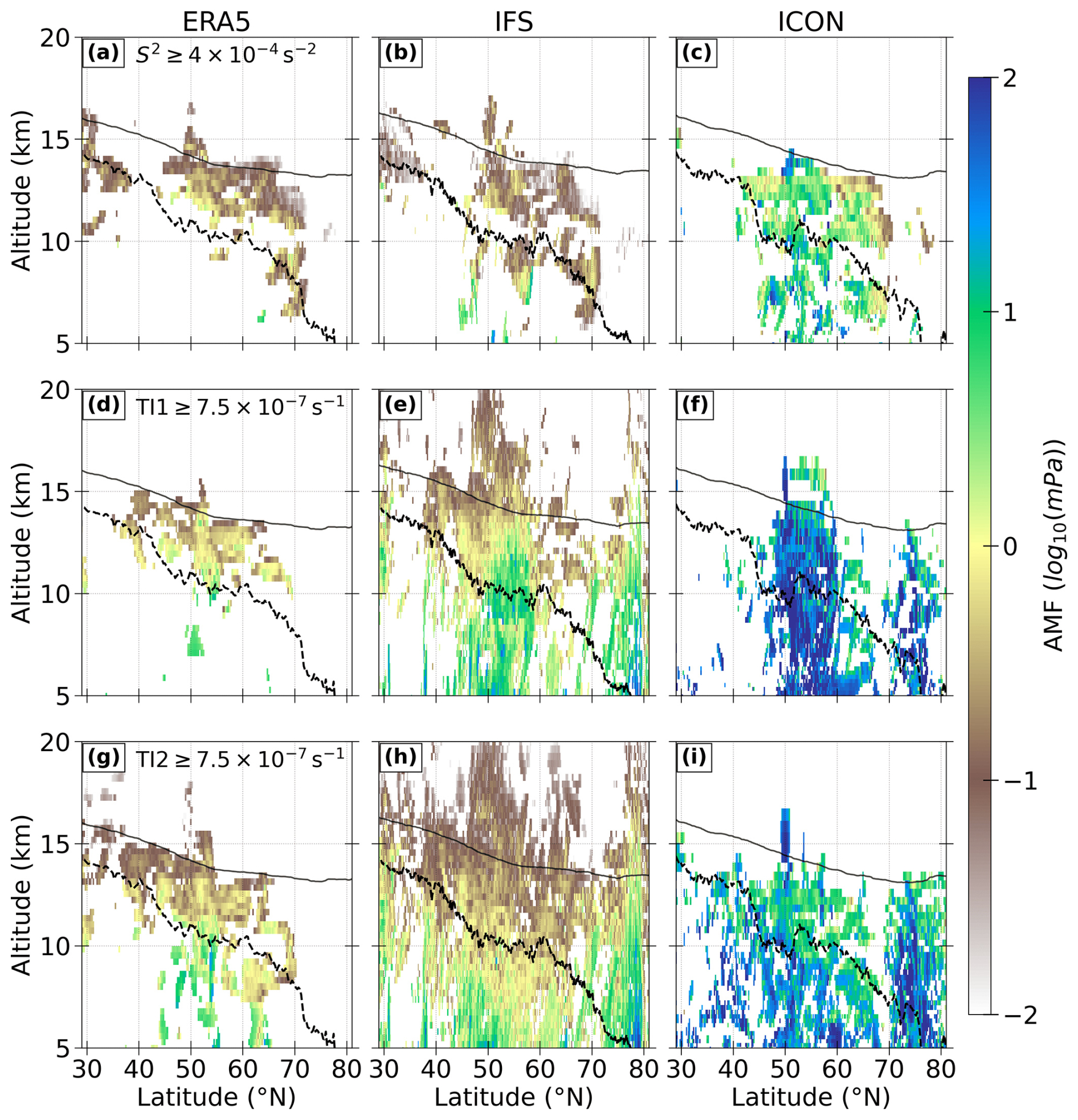
Figure 20 Zonal mean resolved GW absolute momentum flux (AMF, log₁₀(mPa)) values conditioned on regions where (a–c) S² ≥ $S_{\mathrm{t}}^{\mathrm{2}}$, (d–f) $\mathrm{TI}\mathrm{1}\ge \mathrm{7.5}\times {\mathrm{10}}^{-\mathrm{7}}{\mathrm{s}}^{-\mathrm{1}}$ and (g–i) $\mathrm{TI}\mathrm{2}\ge \mathrm{7.5}\times {\mathrm{10}}^{-\mathrm{7}}{\mathrm{s}}^{-\mathrm{1}}$. All values are vertically binned with Δ z = 500 m. The zonal-mean dynamical tropopause (3.5 PVU isosurface; black dashed line) and the zonal-mean 380 K isentrope of potential temperature (solid line) are overlaid.

Finally, the relationship between GWs and CAT is examined using the AMF distribution in the vicinity of enhanced TI1 (Fig. 20d–f) and TI2 (Fig. 20g–i) occurrences. In ERA5, turbulence hotspots largely coincide with enhanced GW activity, with elevated AMF extending across the tropopause into the LMS. The IFS exhibits a broader AMF distribution, characterized by pronounced vertical AMF gradients near elevated TI1 values and a wider spatial extent around TI2 hotspots (Fig. 20e, h). In contrast, the ICON simulation reveals more intense small–scale AMF structures and sharper vertical gradients throughout the UTLS, likely associated with better-resolved GWs (Fig. 20f, i). Overall, enhanced CAT occurrence is consistently accompanied by increased vertical AMF gradients. This spatial correspondence further supports the hypothesis that GW activity contributes to the formation of the observed turbulence hotspots.

Besides this, some uncertainty remains in the quantitative assessment of GW momentum fluxes, as the representation of unresolved wave sources may affect both their magnitude and spatial distribution. It is worth noting that ICON has been shown to reproduce satellite-derived GW momentum flux patterns without requiring additional parameterizations for unresolved waves in the middle stratosphere (Stephan et al., 2019b). However, Toghraei et al. (2025) suggests that its non-orographic parameterizations may underestimate the dynamical filtering of westward-propagating waves in the mid-latitude region. Nonetheless, the co-location of enhanced GW momentum fluxes with regions of elevated TI1 occurrence is consistent with a link between GW activity and CAT generation in the UTLS.

Overall, these findings support the hypothesis that subgrid-scale or small–scale GWs contribute substantially to enhanced shear generation, the development of high-intensity CAT, and consequently are a major part of the dynamics in the ExTL.

7 Discussion and conclusion

The present study highlights the role of gravity wave (GW) induced shear as a key parameter for the tropopause shear layer (TSL, Kaluza et al., 2021), based on observations, reanalysis and forecast data. We show that this mechanism is relevant for the potential occurrence of clear-air turbulence (CAT), which manifests as highly transient yet frequent mixing processes in the extratropical lowermost stratosphere. These processes may therefore play a crucial role in the formation and maintenance of the extratropical transition layer (ExTL), alongside other processes such as convective injection.

Following the results of Umbarkar and Kunkel (2025), we assess whether we can confirm their findings from idealized model studies in a real-world environment over the North Atlantic during an episode of the airborne mission WISE. We use airborne measurements, ERA5 reanalysis, IFS forecast and a comprehensive ICON model forecast for this case study. Using the combination of these datasets allows us to comprehensively study the relationship between vertical shear, GWs and turbulence in the LMS. We combine time series analysis, trace species profiles, tracer-tracer correlations and spectral analysis with a recently explored hybrid approach based on Helmholtz decomposition method (Wei et al., 2022) and come to the following results:

• Airborne observations indicate mixed air masses in regions of enhanced GW activity and vertical shear. We analyzed a WISE campaign flight over the North Atlantic, where tracer–tracer correlations of CO and N₂O revealed such mixed air masses. Vertical profiles of these tracers showed that these air masses were located in the LMS between 345 and 375 K. Further analysis suggests that the mixing was associated with GWs and occurred recently in regions of persistently low Richardson numbers and enhanced vertical wind shear.

• The ERA5 synoptic analysis reveals persistent orographically generated GWs over the Icelandic highlands. Despite its relatively coarse horizontal resolution, ERA5 captures the large-amplitude upward-propagating waves that enhance vertical wind gradients and contribute to shear generation.

• The potential role of GWs in generating shear and turbulence in the LMS is identified through the co-occurrence of small–scale momentum flux, enhanced shear, and low Richardson numbers. GW-induced shear, conducive to turbulence, correlates with envelopes of small–scale GWs (∼ 100 km horizontal wavelength) in the LMS. Spectral analysis indicates a downscale energy transfer from small–scale GWs that intensifies shear near ∼ 340 K, creating conditions favorable for clear-air turbulence. Consistently, turbulence diagnostics, including Ri on larger, and TI1, and TI2 on smaller scales, suggest that GW-induced shear promotes the occurrence of CAT.

• The dynamical situation is similarly represented in ECMWF ERA5 and IFS data. As expected, the higher-resolution IFS reveals more mesoscale structure, while enhanced vertical shear occurs less frequently in ERA5. Nevertheless, ERA5 captures a large part of the GW spectrum and many shear events, making it suitable for long-term analysis of GW-induced shear over the North Atlantic. It is well suited to characterize the large–scale environment and regions favorable for GW activity, but its limited effective resolution constrains particularly the magnitude of small–scale shear and turbulence.

• The high-resolution ICON simulations reproduced the analyzed large-amplitude GW event over the North Atlantic reasonably well. The model simulations indicate that the analysis of GW occurrence and associated vertical shear strongly benefit from finer grid spacings when it comes to the magnitude of the vertical shear. GW activity in the tropopause region is enhanced in convection-permitting simulations, while the GW–shear–turbulence relationship remains similar in convection-parametrized experiments. Compared to ECMWF models, ICON exhibits slightly fewer shear events, suggesting either a redistribution of variance due to resolved small–scale GWs or differences in model formulation and setup.

• Differences in GWs and shear between ECMWF products and ICON are less pronounced in the turbulence indices. Diagnosed turbulent regions show banded structures linked to GWs and GW-induced shear, aligned with upper-level fronts and baroclinic activity (Kaluza et al., 2021). ERA5 and IFS indicate widespread dynamical instability, while ICON shows weaker shear perturbations but higher AMF at low Ri. CAT indices reveal moderate-intensity turbulence in ERA5, with IFS and ICON reproducing this pattern at slightly higher intensity. Overall, GWs play a key role in enhancing shear and CAT in the LMS, and ERA5 is suitable for long-term North Atlantic studies due to its ability to capture GW spectra and their turbulent impact.

The relationship between small–scale GW momentum flux and shear provides a useful diagnostic for assessing GW activity (Plougonven et al., 2003, 2017; Lachnitt et al., 2023; Umbarkar and Kunkel, 2025), and suggests that GWs may contribute to the formation of shear hotspots and irreversible mixing of air masses in the LMS. However, further research should address the seasonal and geographical variability of small–scale, GW–induced shear in the midlatitudes.

The similarities and differences we identified here depend on the model formulation, resolution and parameterization choices. While ICON demonstrates skill in reproducing GW flux patterns comparable to those in IFS, questions remain as to whether resolved GW amplitudes in the extratropics have fully converged across resolutions, and how parameterized sources interact with the resolved wave spectrum. This uncertainty is supported by the fact that high-resolution simulations have not yet converged when it comes to GWs in the extratropics (Kruse et al., 2022; Polichtchouk et al., 2023; Gupta et al., 2024).

Our results suggest a multiscale cascade in which orographically generated inertia–gravity waves enhance shear, contribute to the development of small–scale instabilities, and promote turbulence, thereby facilitating vertical energy and momentum transfer. GW-induced shear emerges as an important mechanism influencing UTLS transport, mixing, and CAT occurrence. This findings motivate further investigation of its regional prevalence and implications for the redistribution of H₂O and O₃ and associated radiative forcing (e.g., Riese et al., 2012), as well as aviation forecasting (e.g., Kim and Chun, 2011; Sharman and Pearson, 2017). Overall, GW-related processes are an important framework for understanding CAT in the extratropical UTLS.

Appendix A: Supporting figures to selected methodology, synoptic situation and hodograph analysis

Figure A1 Vertical cross section of zonal wind u (upper panel) and retrieved u perturbations (lower panel) on 23 September 2017 11:00 UTC at 20° W for (a, d) ICON, (b, e) ERA5, and (c, f) IFS.

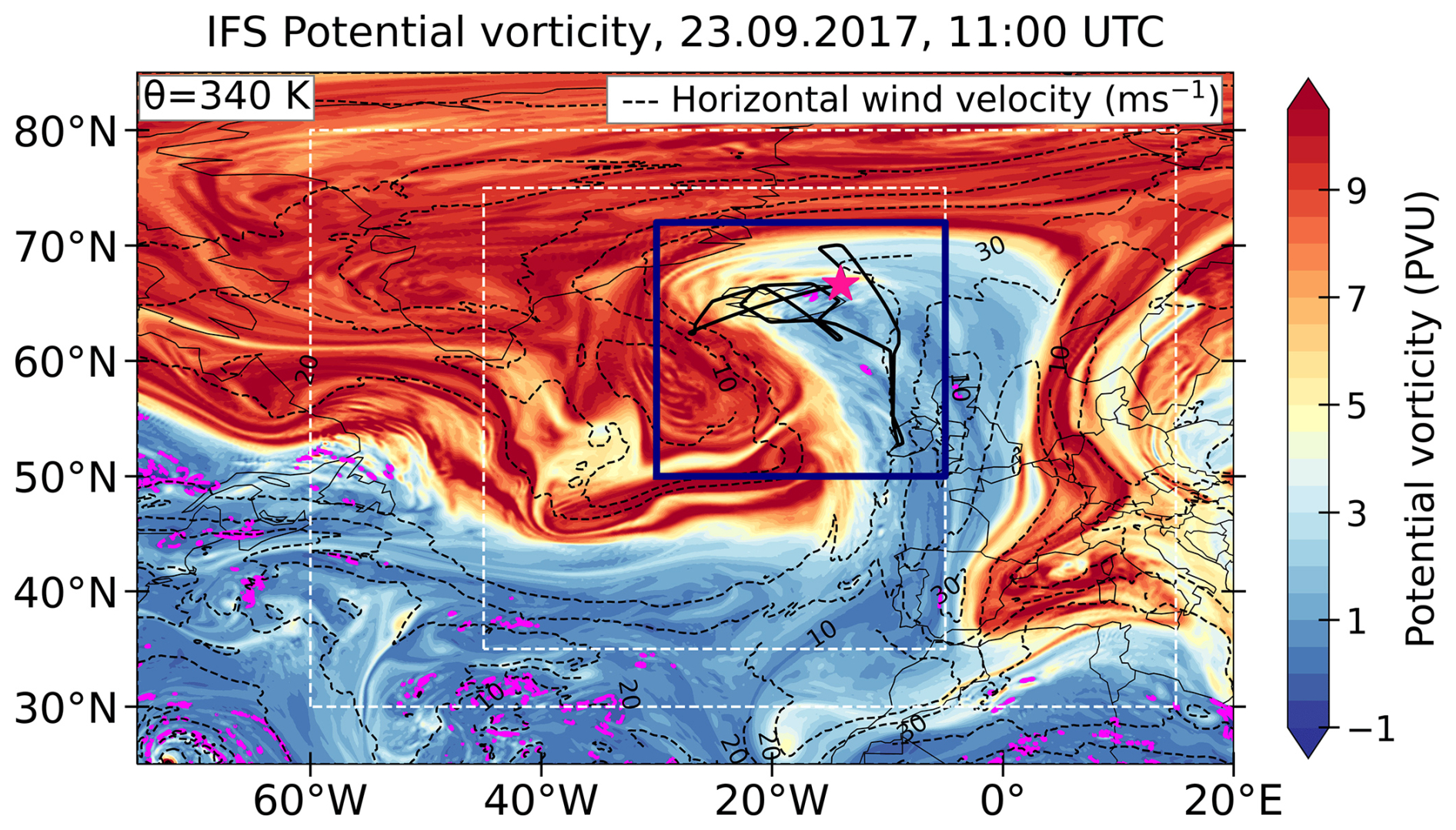
Figure A2 IFS potential vorticity distribution (in PVU) at the 340 K isentropic surface on 23 September 2017 at 11:00 UTC. The dashed lines show the horizontal wind (in m s⁻¹) on 340 K. The thick black line shows the flight path of RF05 and the star marks the aircraft position at 11:00 UTC. Magenta color shows the negative PV values.

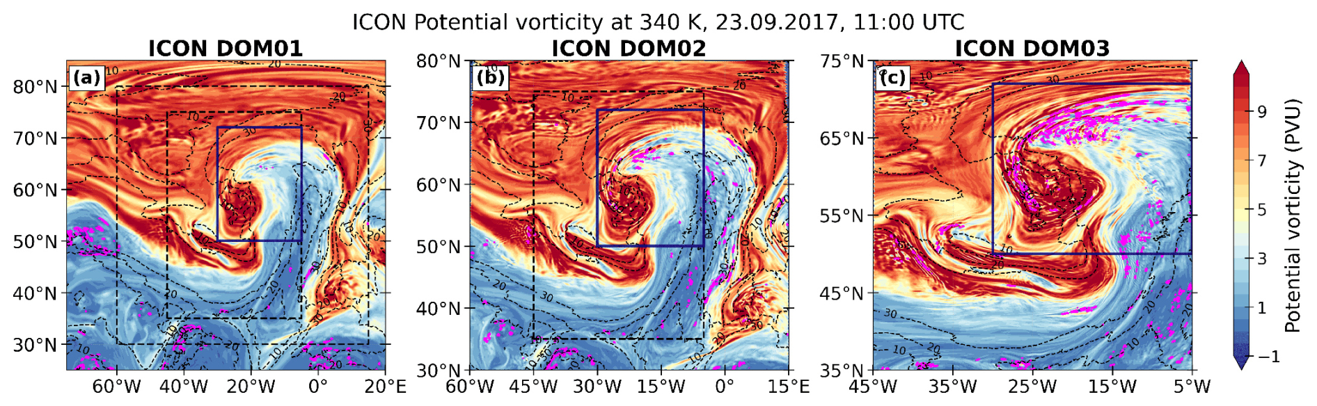
Figure A3 Potential vorticity distribution (in PVU) at the 340 K isentropic surface on 23 September 2017 at 11:00 UTC for three ICON domains: (a) ICON 13 km (b) ICON 6.5 km and (c) ICON 3.3 km. The dashed lines show the horizontal wind (in m s⁻¹) on 340 K. Magenta color shows the negative PV values, while blue box represent analysis domain selected for this study.

Figure A4 Time series of (a) zonal (u, m s⁻¹; blue) and meridional (v, m s⁻¹; red) wind component from HALO for WISE RF05, the shaded yellow regions same as Fig. 3, whereas panel (b) shows perturbation of u and v obtained from Butterworth filter.

Appendix B: Supporting information to the GW and shear analysis

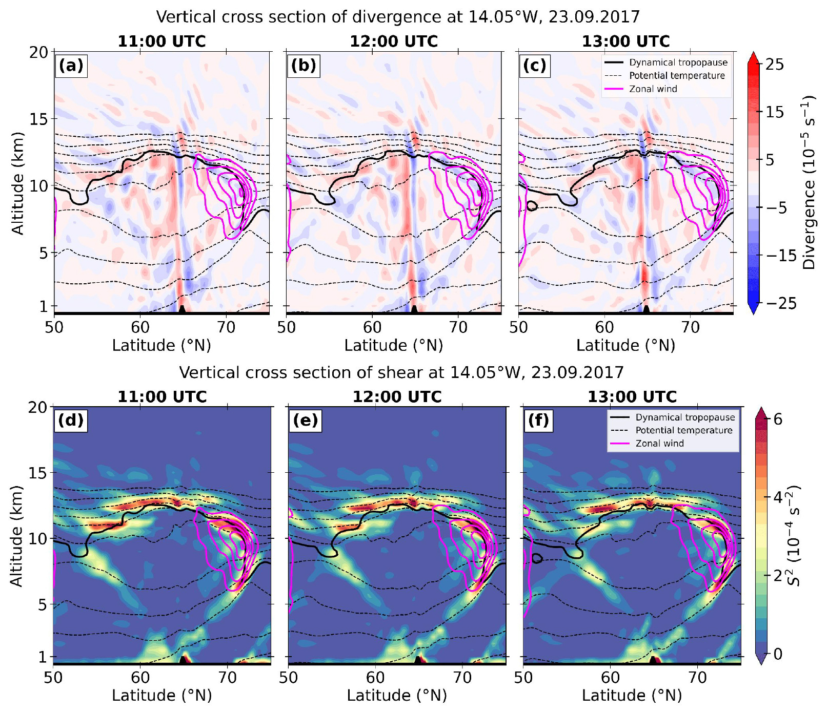
Figure B1 Vertical cross sections of divergence (a–c) and vertical shear (d–f) at longitude 14.05° W for ERA5 data at 11:00, 12:00 and 13:00 UTC. The solid black line represent the 3.5 PVU as a dynamical tropopause whereas dashed lines in lower panel represent the potential temperature starting from 280 K (bottom) to 380 K (top) with 10 K increments.

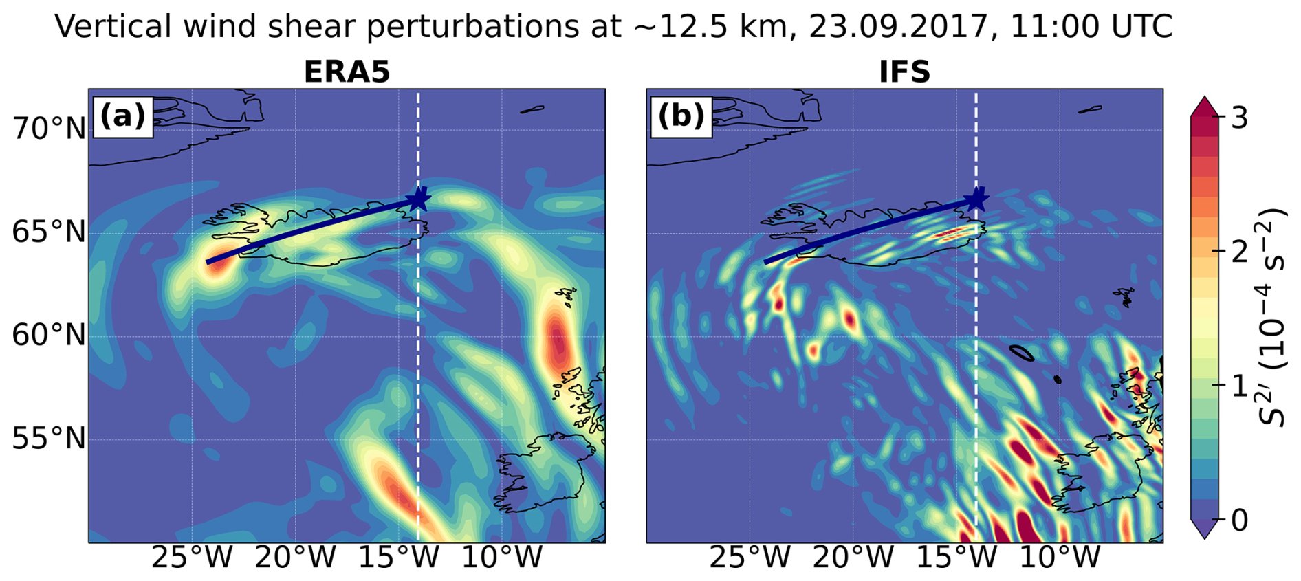
Figure B2 Distribution of vertical wind shear perturbations $S^{{\mathrm{2}}^{\prime }}$ at ∼ 12.5 km altitude for (a) ERA5 and (b) IFS.

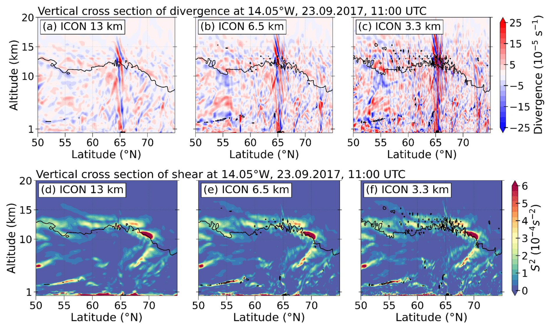
Figure B3 Vertical cross sections of divergence (a–c) and vertical shear (d–f) at longitude 14.05° W for three ICON domains. The solid black line represent the 3.5 PVU as a dynamical tropopause.

Appendix C: Supporting information to the CAT analysis

We use all data points in the LMS i.e., between 3.5 PVU and 380 K, to derive PDF distribution of the small–scale TI1 and TI2 indices. We then calculate the 95th percentile values of these distributions, which are used as threshold values. The resulting TI1 threshold values for ERA5, IFS and ICON are $\mathrm{1.4}\times {\mathrm{10}}^{-\mathrm{7}}$, $\mathrm{2.1}\times {\mathrm{10}}^{-\mathrm{7}}$ and $\mathrm{1.5}\times {\mathrm{10}}^{-\mathrm{7}}{\mathrm{s}}^{-\mathrm{1}}$ respectively. There are only minor difference in the threshold across the datasets. Given the range of values in PDFs and the differences in the underlying data, the gained thresholds differ only slightly across the datasets, with some differing up to a factor of two.

Furthermore, the more GW-related index TI2 applies the same threshold criterion as TI1, where the resulting thresholds are $\mathrm{1.5}\times {\mathrm{10}}^{-\mathrm{7}}$, $\mathrm{2.45}\times {\mathrm{10}}^{-\mathrm{7}}$, and $\mathrm{1.5}\times {\mathrm{10}}^{-\mathrm{7}}{\mathrm{s}}^{-\mathrm{1}}$ for ERA5, IFS and ICON, respectively. We categorize the CAT levels based on the thresholds: light to moderate from respective 95th percentile threshold, moderate (7.5 $\times {\mathrm{10}}^{-\mathrm{7}}$ to 12$\times {\mathrm{10}}^{-\mathrm{7}}{\mathrm{s}}^{-\mathrm{1}}$), and moderate-or-greater (> 12 $\times {\mathrm{10}}^{-\mathrm{7}}{\mathrm{s}}^{-\mathrm{1}}$), consistent with previous studies (e.g., Ellrod and Knapp, 1992; Thompson and Schultz, 2021).

Figure C1 Relative occurrence frequency distribution of (a) TI1 and (b) TI2 for ERA5, IFS and ICON in the LMS domain. Corresponding to histogram, colored dashed lines indicate threshold retrieved as the 95th percentile over the LMS domain that is considered as threshold for light moderate category. Grey and aqua lines represent the threshold for moderate (7.5–12 $\times {\mathrm{10}}^{-\mathrm{7}}{\mathrm{s}}^{-\mathrm{1}}$) and moderate to greater (moderate to greater; > 12 $\times {\mathrm{10}}^{-\mathrm{7}}{\mathrm{s}}^{-\mathrm{1}}$) intensity clear air turbulence, respectively.

ICON sensitivity: CAT threshold selection

The relative occurrence frequency distributions of TI1 and TI2 for the three ICON domains in the LMS are shown in Fig. 17. The threshold criterion is based on 95th percentile for each case in the LMS and is same as in ERA5. The resulting TI1 threshold values for simulations with Δx≈13, Δx≈6.5, and Δx≈3.3 km are $\mathrm{1.5}\times {\mathrm{10}}^{-\mathrm{7}}$, $\mathrm{3.21}\times {\mathrm{10}}^{-\mathrm{7}}$, and $\mathrm{4.03}\times {\mathrm{10}}^{-\mathrm{7}}{\mathrm{s}}^{-\mathrm{1}}$, respectively; and for TI2, the resultant threshold values are $\mathrm{1.72}\times {\mathrm{10}}^{-\mathrm{7}}$, $\mathrm{3.75}\times {\mathrm{10}}^{-\mathrm{7}}$, and $\mathrm{4.31}\times {\mathrm{10}}^{-\mathrm{7}}{\mathrm{s}}^{-\mathrm{1}}$, respectively. For the comparison across experiments and following the previous studies (e.g.,  Thompson and Schultz, 2021), the threshold values are kept common for moderate (7.5–$\mathrm{12}\times {\mathrm{10}}^{-\mathrm{7}}{\mathrm{s}}^{-\mathrm{1}}$) and moderate-to-greater ($>\mathrm{12}\times {\mathrm{10}}^{-\mathrm{7}}{\mathrm{s}}^{-\mathrm{1}}$) categories.

Appendix D: Supporting information to “Turbulence diagnostics in a zonal framework”

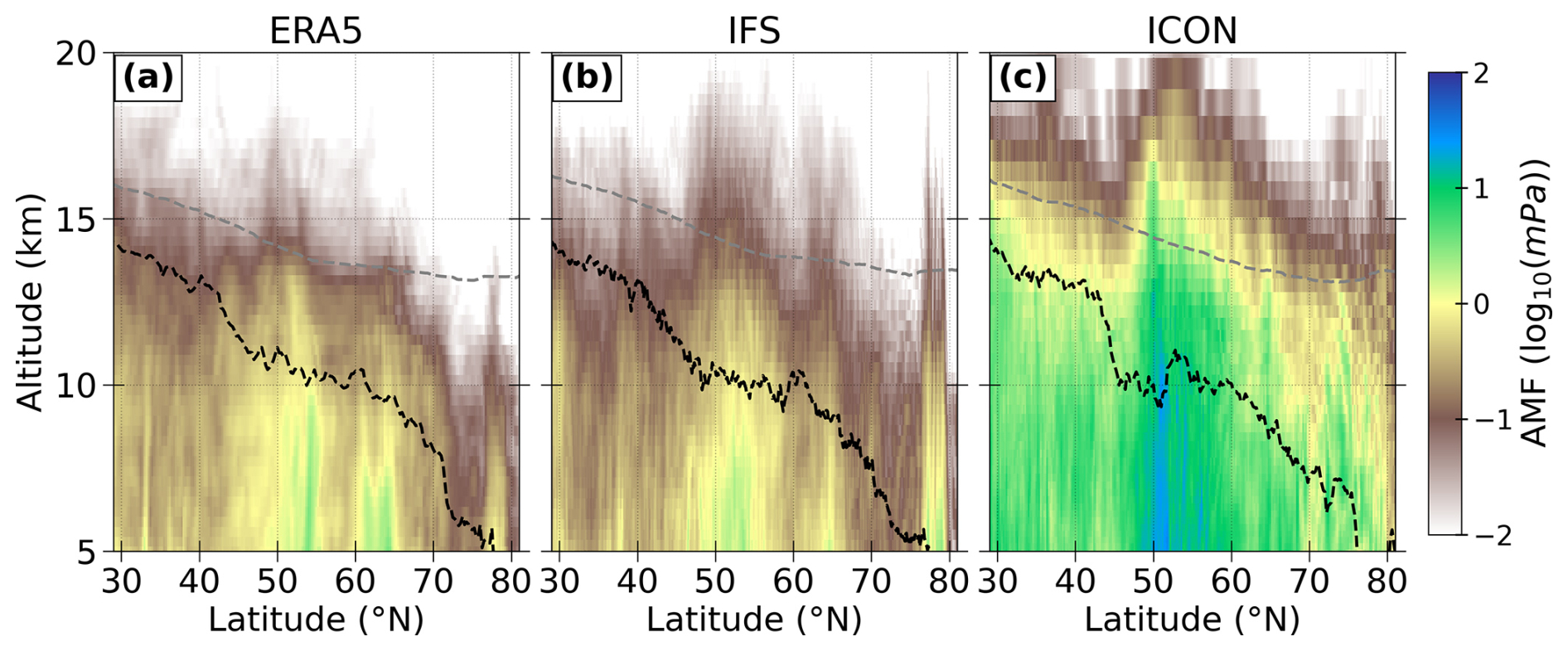
Figure D1 Zonal mean GW absolute momentum flux (AMF, log₁₀(mPa)) for (a) ERA5, (b) IFS and (c) ICON ≈13 km resolution simulation.