Impact of South American biomass burning emissions on elevated South Atlantic upper tropospheric ozone

During the SOUTHTRAC mission in autumn 2019 elevated mixing ratios of carbon monoxide (CO), carbon dioxide CO₂, nitrogen oxide (NO) and total reactive nitrogen NO_y were observed during a flight at the beginning of October. The potential plume extended over more than 1000 km (15° latitude) east of the Brasilian coast at altitudes of 13 km in the upper troposphere. In-situ measurements showed elevated ozone in this plume (≈ 100 ppbv), being 20–40 ppbv higher than during a previous flight in early September at exactly the same flight route. For the plume flight positive correlations of ozone and pollutants (CO, NO, NO_y) indicate ozone production in these pollution layers. Lagrangian Analysis shows, that the observed air masses were strongly affected by biomass burning over Amazonia. A combined analysis of a chemical Lagrangian box model and a global chemistry climate model (EMAC) revealed that ozone production from biomass burning predominantly caused the ozone enhancements. The effect is intensified by NO_x produced from lightning. Upward transport of the plumes happened ≈ one week before the flight, allowing ozone to be formed and enhanced by 25 % compared to the September flight.

Estimate of the potential climate impact show, that the biomass burning produced ozone has an impact on the radiation budget, namely a spatially and regionally localized radiative flux disturbance of up to 250 mW m⁻² at the tropopause and 150 mW m⁻² at the top of the atmosphere.

1 Introduction

Ozone (O₃) is one of the most important anthropogenic greenhouse gases besides carbon dioxide (CO₂) and methane (CH₄) but has a larger uncertainty in its radiative forcing partly because of the highly variable source characteristics of ozone precursor gases such as nitrogen oxides ($\mathrm{NO}+{\mathrm{NO}}_{\mathrm{2}}={\mathrm{NO}}_x$) and volatile organic compounds (VOCs). This holds in particular for wildfire emissions as well as the production strength of nitrogen oxides by lightning (LNO_x).

Biomass burning is an important source for tropospheric O₃ (Mauzerall et al., 1998; Duncan et al., 2007; Andreae, 2019; Schill et al., 2020) underlying however, strong regional and seasonal changes. Jaffe and Wigder (2012) estimate that approximately 3.5 % of global tropospheric O₃ formation is related to biomass burning emissions. Since the wildfire activity is projected to increase (Jacob and Winner, 2009; Torres et al., 2010; Yue et al., 2015; Abram et al., 2021), this source of O₃ will be more important in the future.

Trace gases emitted by fires can be transported into the upper troposphere and lower stratosphere (UTLS) and produce O₃ which acts as a greenhouse gas in these altitudes (Rap et al., 2015; Bozem et al., 2017; Xia et al., 2018; Bourgeois et al., 2021). Thus, perturbations of upper tropospheric (UT) ozone play an important role for the radiation budget of the atmosphere (Forster and Shine, 2002; Riese et al., 2012). Notably in the tropics and subtropics the impact of UT ozone on the local energy budget can be substantial (Rap et al., 2015).

To identify ozone production in observational data sets, positive correlations between O₃ and CO can be used. This is due to the fact that CO, NO_x and other ozone precursors are co-emitted by biomass burning as well as anthropogenic pollution sources. However, the correlation between O₃ concentrations and biomass burning (BB) emissions is complex and highly non-linear leading mainly to ozone depletion in regions closer to the fire (e.g. Wentworth et al., 2018). Ozone production occurs mainly in larger distances downwind the fire, in particular in the mid- and upper troposphere (Real et al., 2007; Akagi et al., 2012; Parrington et al., 2013). The wide variation in net O₃ production within biomass burning smoke is related to several factors, including fire temperature, burning material and therefore differing emissions with respect to the emission strength as well as the ratios of the emitted species, all in combination with the prevailing meteorological conditions (e.g. Gilman et al., 2015; Koss et al., 2018; Andreae, 2019). Each of these factors influence the underlying RO_x (${\mathrm{RO}}_x=\mathrm{OH},{\mathrm{HO}}_{\mathrm{2}}$, and RO₂) chemistry that controls oxidation processes and secondary pollutant formation. Direct HO_x precursor emissions like formaldehyde (HCHO), acetaldehyde (CH₃CHO), and nitrous acid (HONO) show a great variability depending on the fire type and fire state (Liao et al., 2021; Kluge et al., 2020; Fiddler et al., 2024).

Tropospheric O₃ formation generally depends on the availability of NO+NO₂ (NO_x) and volatile organic compounds (VOCs) in the atmosphere (Leighton, 1961; Crutzen, 1974). It is common to divide O₃ formation regimes into NO_x sensitive (increase in NO_x leads to increase of O₃, changes in VOC's have little to no impact on O₃ mixing ratios) or VOC sensitive (further increase of NO_x leads to decrease of O₃) (Sillman, 1999). The resulting O₃ isopleths as a function of NO_x and VOC mixing ratios are often used to explain the different O₃ formation regimes (e.g. Seinfeld and Pandis, 2016). However, for a large range of scientific data analysis applications they are not applicable since (i) a large (box model) dataset is required to compose an O₃ isopleth diagram, (ii) knowledge of the mixing ratios of all atmospheric VOC compounds is hypothetically required, (iii) the method has been developed for (boundary layer) urban air pollution and is not necessarily applicable in the upper troposphere (Nussbaumer et al., 2023). Several approaches to use trace gas or production rate ratios as indicators for O₃ formation regimes have been developed in the past (e.g. Sillman, 1995; Tonnesen and Dennis, 2000; Tadic et al., 2020), but most of them are again not suitable for applications in the upper troposphere (Nussbaumer et al., 2023).

More than three decades ago, Fishman et al. (1990) and Watson et al. (1990) detected an O₃ maximum over the southern hemispheric Atlantic by using TOMS satellite data. Observational data from the SHADOZ network (Sauvage et al., 2006; Thompson et al., 2017; Witte et al., 2017), satellite data (Edwards et al., 2003) and simulations with a global chemical transport model (Moxim and Levy, 2000) indicate, that the region with elevated column O₃ level stretch over almost the entire tropical and northern sub-tropical South Atlantic. Convective uplift of biomass burning emissions (Chatfield and Delany, 1990; Pickering et al., 1992; Kirchhoff and Marinho, 1994), the formation of nitrogen oxides by lightning (LNO_x) and long-range transport from South America and Africa to the Atlantic are supposed to contribute to the wave-one ozone maximum developing during September, October and November (SON) in the troposphere (Jenkins et al., 1997, 2021). The biomass burning season in South America is mainly concentrated between July and October, a period characterized by dry conditions associated with the decay phase of the South American monsoon system (Vera et al., 2006) while lightning activity reaches its maximum in SON over South America (Jenkins and Ryu, 2004). The number of convective events is largest in austral summer (DEC-FEB) however, they occur numerously and with a high variability with respect to the location and strength in all seasons. The relative contribution of biomass burning and LNO_x for the development of the South-Atlantic O₃ maximum is however, unclear (Edwards et al., 2003; Jenkins and Ryu, 2004; Sauvage et al., 2006; Jenkins et al., 2021). Using aircraft data over Brazil, trajectory data and ozone sonde data along the South-American east coast, Pickering et al. (1996) found evidence that uplift of biomass burning emissions in the vicinity of convective clouds in combination with lightning are the driving processes leading to the O₃ maximum over the SW-Atlantic. Pickering et al. (1996) estimate that the lightning contribution amounted to at least 32 % of the measured NO_x mixing ratios.

For the tropical south Atlantic, Murray et al. (2013) estimate that LNO_x emissions are by far more important for O₃ production than biomass burning. Next to long range transport of biomass burning emissions and lightning NO_x production, downward transport of stratospheric air masses could contribute to the observed O₃ maximum. However, Liu et al. (2017) find that the contribution of biomass burning surface emissions exceed stratospheric impacts on O₃ formation over the northern South Atlantic.

Ulke et al. (2011) investigate transport patterns of biomass burning emissions from amazon forest fires. They conclude that in addition to convective uplift, the South American Low Level Jet (SLLJ) (Liebmann et al., 2004; Vera et al., 2006), a northerly wind east of the Andes mountains is all year round an important transport pathway of moisture and trace species from the Amazon to SE South America.

During austral summer, a band of high (convective) clouds develop regularly along the of South Atlantic Convergence Zone (SACZ) expanding from North-West Brazil (Amazon fire regions) to South-East Brazil. The SACZ can last quasi stationary for up to 8 d during austral summer, but it develops less intense also in austral spring (Liebmann et al., 2004; de Oliveira Vieira et al., 2013; Villela, 2017), representing another potential upper tropospheric outflow path for amazon BB emissions.

Motivation and objective

The SOUTHTRAC mission was carried out from September 2019 to November 2019 and consisted of two phases, with the HALO aircraft based in Rio Grande (Argentina) (Rapp et al., 2021). Inbetween the two phases HALO returned back to Germany, with the long transsects between South America and Germany carried out as measurement flights. This provided several long flight legs in the UTLS across the Atlantic, on which we will focus here.

During a flight at the beginning of October elevated upper tropospheric mixing ratios of CO, NO, NO_y and O₃ were observed. The plume extended over more than 1000 km (15° latitude) east of the Brasilian coast. Measured O₃ mixing ratios in this plume (≈100 ppbv), are about 20–40 ppbv higher than during a previous flight in early September at exactly the same location and altitude range. The objective of our work is to locate the source region of the pollution layer and to quantify the contribution of biomass burning and lightning NO_x emissions to O₃ production by combining the observations obtained during the SOUTHTRAC mission and a set of model simulations.

2 Data and Methods

2.1 Instrumentation

HALO is capable of reaching flight altitudes of 14.5 km (49 000 ft.) corresponding to pressure levels of 150 hPa. The aircraft was equipped with a comprehensive payload combining remote sensing and in-situ instruments. We focus here on in-situ measurements of carbon monoxide (CO), carbon dioxide (CO₂) as well as ozone (O₃). CO and CO₂ were measured with the UMAQS instrument (University Mainz Airborne Quantum Cascade Laser Spectrometer) from Johannes Gutenberg university Mainz (Müller et al., 2015; Kunkel et al., 2019). The instrument is in-situ calibrated against two secondary standards of different mixing ratios, which are compared to NOAA primary standards prior and after the campaign. Calibrations are carried out every 30–45 min to account for drifts of the instrument due to temperature driven changes of the optical path or the electronics. UMAQS is equipped with two astigmatic Herriot cells with an optical path lengths of 76 m (McManus et al., 2005). Cell pressure is stabilized at a cell pressure of 50 hPa. The time resolution is ultimately limited by the gas exchange rate in the cell as given by the pump speed and was at 1.5 s during SOUTHTRAC. Estimated accuracy at flight level is 2.5 ppbv for CO with a 1σ precision of 2 ppbv for CO. Ozone was measured with the Fast Airborne Ozone instrument (FAIRO), which combines UV photometry and chemoluminescence (Zahn et al., 2012). The time resolution is at 10 Hz, which is averaged to 1 s using a simple boxcar average giving an overall uncertainty of 2 % for ozone. Total reactive nitrogen (NO_y) and nitrogen oxide (NO) were measured by the AENEAS instrument (Ziereis et al., 2022). The overall uncertainty of the total reactive nitrogen measurement depends on the actual ambient concentration. It is about 8 % for volume mixing ratios of 0.5 ppb and about 6.5 % for about 1 ppb (Ziereis et al., 2022, and references therein).

2.2 Satellite data

2.2.1 MOPITT satellite data

To analyse upper tropospheric CO level over South America, we use thermal infrared level 3 data from the version 8 product of CO measurements derived from the MOPITT instrument (Deeter et al., 2019). Level 3 products are available as daily mean values on a 1° × 1° global grid.

2.2.2 GOES satellite data

To identify fire and lightning events, we use GOES-16 satellite data. GOES-16 is one of NOAA's geostationary satellites centered over 75° W, having a hemispheric coverage of 83° local zenith angle on the full disk mode providing observation measurements between 52° North and South. GOES-16 data cover the north- and south American continents and the adjacent oceans.

The Advanced Baseline Imager (ABI) is a 16-channel (2 visible, 4 nearinfrared, 10 infrared) passive imaging radiometer on board GOES-16. The Fire Detection and Characterization (FDC) product is one of the multiple GOES-16 ABI-derived baseline products (GOES-R Series Program, 2019) It provides imagery of the Earth's surface and the atmosphere at very high spatial (2 km for infrared bands) and temporal (5 min) resolutions. Under clear-sky conditions, the minimum detectable size of a fire (mean temperature: 800 K) is estimated to be 0.004 km² at the sub-satellite point. It provides fire detection locations (latitude, longitude) and fire properties such as the fire radiative power.

The GOES-R Geostationary Lightning Mapper (GLM) instrument on board GOES-16 (GOES-R Algorithm Working Group and GOES-R Series Program, 2018) is a single-channel, near-infrared optical transient detector that can detect the instantaneous changes in an optical scene, indicating the presence of lightning. GLM provides data of in-cloud, cloud-to-cloud and cloud-to-ground lightning activity with a spacial resolution of approximately 10 km and a temporal resolution of 20 s.

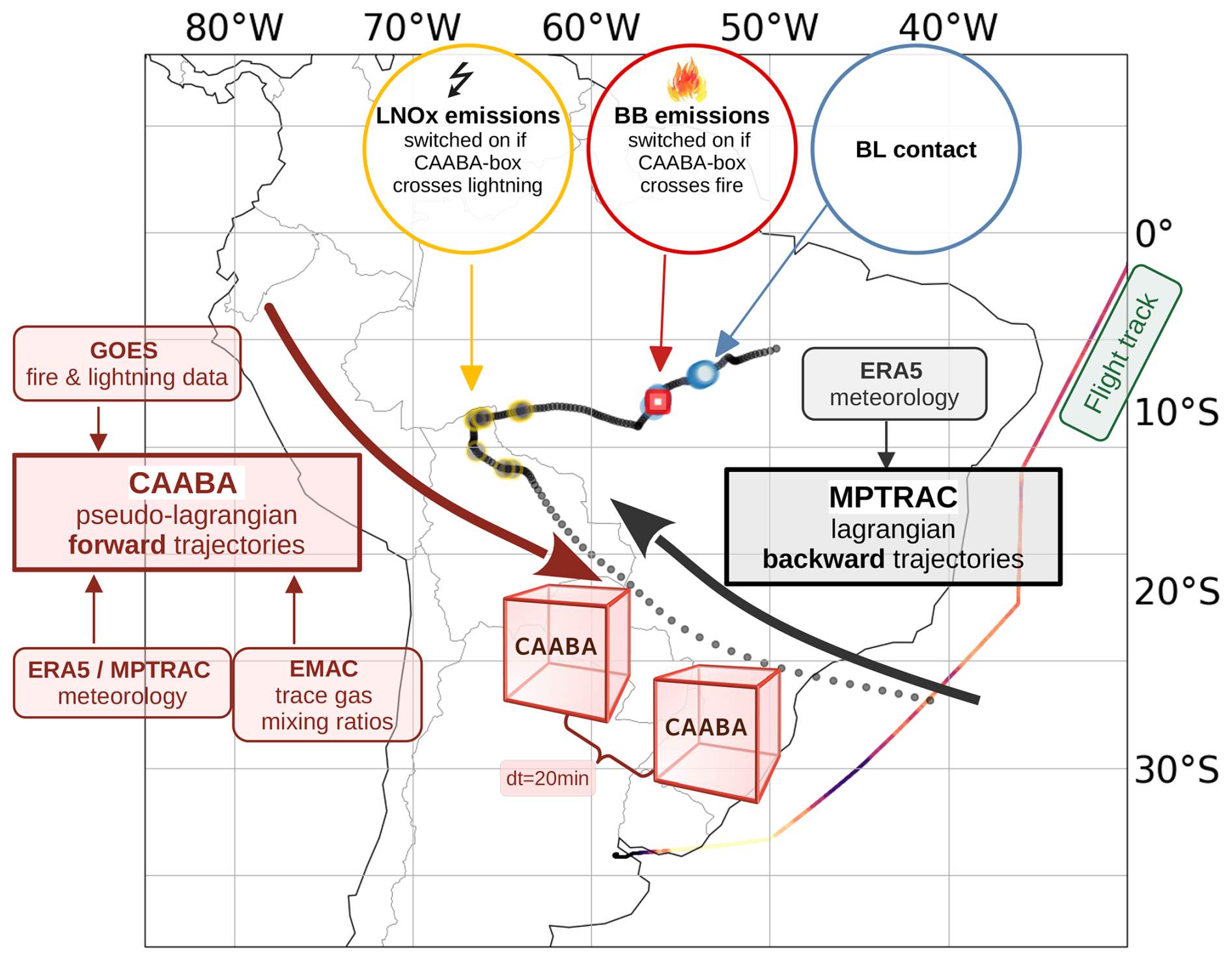
Figure 1 Schematic overview of the CAABA simulation setup.

2.3 Model description

To simulate the chemical and dynamical history of air masses being sampled along the HALO flight track, we use a combination of different model- and satellite data products.

2.3.1 Kinematic trajectory setup

To analyse the dynamical history of air masses, we calculate backward trajectories using MPTRAC (Hoffmann et al., 2016, 2022) which is a massive-parallel Lagrangian particle dispersion model allowing a computationally efficient calculation of transport simulations in the troposphere and stratosphere. A cluster of 240 trajectories is started every 5 min in a square of 0.25° surrounding the flight track. The backward simulation time of each trajectory is 13 d. MPTRAC simulations are driven with meteorological data from the ECMWF (European Center for Medium-Range Weather Forecast) ERA5 atmospheric reanalysis data set (Hersbach et al., 2020).

The ERA5 based MPTRAC simulations do not explicitly represent deep convection since trajectory calculations are only driven by large scale wind fields. Lawrence and Salzmann (2008) point out that trajectories should represent the net vertical and long-range transport reasonably. As Lawrence and Salzmann (2008) and Lawrence and Lelieveld (2010) discuss in detail, it can be assumed that the basic regional lofting is present in lagrangian trajectory simulations but it has to be expected that the mean rate of vertical transport is underestimated. A more recent study by Smith et al. (2021) indicates that a significant portion of convective transport processes are represented in trajectory experiments driven by the grid scale wind fields. They further conclude, that convective and boundary layer source regions of upper tropospheric air parcels are consistent with the climatological flow regime in their study region.

2.3.2 Chemical Lagrangian analysis

To analyse the chemical processing of air masses before they reach the flight path, we use the chemical box model CAABA (Sander et al., 2019) in a pseudo-lagrangian way to calculate atmospheric chemistry along each trajectory calculated with MPTRAC (Fig. 1). Chemistry simulations using the CAABA box model are initiated at the last MPTRAC timestep. For trajectories having boundary layer contact over the South American continent, CAABA simulations are initiated 24 h before the first BL contact. CAABA is calculated every 20 min in the forward mode along each trajectory until the flight path is reached (see Fig. 1). The procedure is similar as in Riede et al. (2009) but with numerous extensions in CAABA: (i) Meteorological conditions (temperature, pressure, humidity, geographical position of the air mass) used in CAABA are taken from the trajectories calculated with MPTRAC (i.e. ERA5 meteorology). (ii) Gas phase chemistry is calculated using MECCA/MIM (Pöschl et al., 2000; Sander et al., 2019) which is the same chemical mechanism as used by EMAC and as applied by Nussbaumer et al. (2023). (iii) Chemical trace species are initialised with mixing ratios obtained from a simulation with the EMAC model (Jöckel et al., 2016) with a resolution of T42L90MA (i.e., ≈2.8125° × 2.8125°) similar as in Jöckel et al. (2016). (iv) We implemented an algorithm, to account for turbulent mixing of air masses in the CAABA-box with background air masses outside the chemical box model. For ambient trace gas mixing ratios we use again data from the EMAC simulation. The mixing strength is scaled with the Richardson number which is calculated based on ERA5 data. (v) Aerosol phase chemistry is not calculated explicitly but heterogeneous reactions on aerosol particles are parameterised using a climatological aerosol size distribution obtained again from EMAC data. (vi) To calculate photolysis rates in CAABA/MECCA, ERA5 cloud data and O₃ column data from EMAC are used. (vii) Anthropogenic emissions from the IPCC RCP6.0 emission inventory are used (Pozzer et al., 2009; van Vuuren et al., 2011). All required quantities (satellite data products, 3D-model data) are sampled and interpolated to the trajectory position in space and time.

The calculation of biomass burning emissions follows the procedure of Kaiser et al. (2012). However, we use instantaneous fire radiative power data from the GOES satellite instead of the assimilated GFAS product (Eqs. 35, 36 in Kaiser et al., 2012). The dry matter combustion rate f(DM) for each located fire is calculated as

$$\begin{array}{}\text{(1)}& f\left(\text{DM}\right)=\sum _{i=\mathrm{1}}^{\mathrm{8}}{\mathit{\delta }}_{i,l}{\mathit{\beta }}_i\mathit{\rho }\end{array}$$

where ρ is the fire radiative power, l, i∈[1,8] denotes the land cover class at the fire location which is taken from Table 2 in Kaiser et al. (2012) like the conversion factor β. The emission rate density f(s) for smoke constituents s is defined as:

$$\begin{array}{}\text{(2)}& f\left(s\right)=\mathit{\kappa }\left(s\right)f\left(\text{DM}\right)\end{array}$$

The species emission factors (κ) are taken from Andreae and Merlet (2001) with updates from Akagi et al. (2011). The technical implementation of biomass burning emissions into CAABA follows Cabrera-Perez et al. (2016). Biomass burning emissions in CAABA are switched on, if air masses cross a fire detected by GOES and air masses are within the (ERA5) boundary layer (BL).

Subsequently lightning NO_x emissions are switched on in CAABA, if the trajectory crosses a lightning event detected by the GLM sensor on board GOES-16. In this case, a constant emission of 0.02 ppb is added to the NO concentration in CAABA (see Fig. 1).

2.3.3 O₃ production metric

Due to the deficiencies of current metrics to classify ozone production regimes in the UT, Nussbaumer et al. (2022) have developed a novel method to investigate O₃ formation regimes which is still valid outside the atmospheric boundary layer. Their method is based on the idea, that O₃ formation in the upper troposphere can be described by the reaction between NO or HO₂ and peroxy radicals, the latter being approximated by CH₃O₂ accounting for ≈85 % of all peroxy radicals in the upper troposphere (Nussbaumer et al., 2021, 2023). While the production of HCHO via reaction of CH₃O₂ with NO or OH enhances O₃ formation, the reaction between CH₃O₂ and HO₂ leads to the formation of CH₃OOH terminating the HO_x cycle and leading to a deceleration of O₃ formation. This relationship is defined by Nussbaumer et al. (2023) with the term ${\mathit{\alpha }}_{\left({\mathrm{CH}}_{\mathrm{3}}{\mathrm{O}}_{\mathrm{2}}\right)}$

$$\begin{array}{}\text{(3)}& \begin{array}{rl}& {\mathit{\alpha }}_{\left({\mathrm{CH}}_{\mathrm{3}}{\mathrm{O}}_{\mathrm{2}}\right)}\\ & ={\displaystyle \frac{k_{({\mathrm{CH}}_{\mathrm{3}}{\mathrm{O}}_{\mathrm{2}}+\mathrm{NO})}\cdot \left[\mathrm{NO}\right]+k_{({\mathrm{CH}}_{\mathrm{3}}{\mathrm{O}}_{\mathrm{2}}+\mathrm{OH})}\cdot \left[\mathrm{OH}\right]}{k_{({\mathrm{CH}}_{\mathrm{3}}{\mathrm{O}}_{\mathrm{2}}+\mathrm{NO})}\cdot \left[\mathrm{NO}\right]+k_{({\mathrm{CH}}_{\mathrm{3}}{\mathrm{O}}_{\mathrm{2}}+\mathrm{OH})}\cdot \left[\mathrm{OH}\right]+k_{({\mathrm{CH}}_{\mathrm{3}}{\mathrm{O}}_{\mathrm{2}}+{\mathrm{HO}}_{\mathrm{2}})}\cdot \left[{\mathrm{HO}}_{\mathrm{2}}\right]}}\end{array}\end{array}$$

where k is the rate coefficient for the reactions given in the brackets. Note, that the reaction between CH₃O₂ and OH is not included in the MIM chemical reaction mechanism due to its slow turnover time.

2.3.4 CAABA simulation scenarios

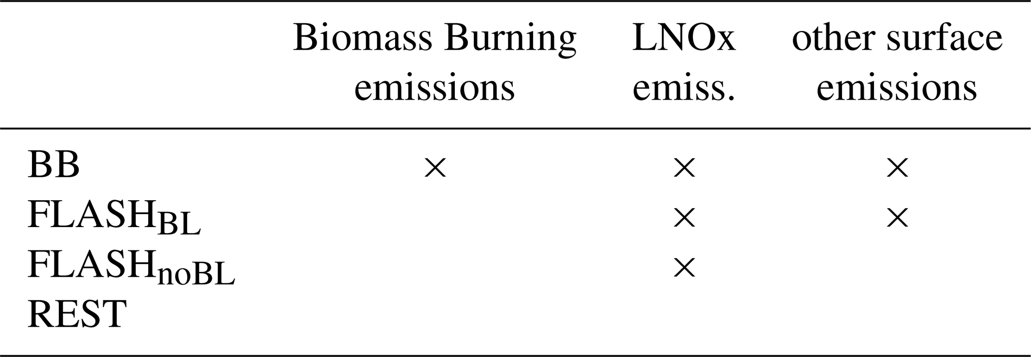
To analyse MPTRAC/CAABA trajectories, we assort them into different categories. Trajectories which (i) cross fires while they are in the BL (BB, all of these trajectories also cross lightning regions), (ii) cross lightning regions with previous continental BL contact (FLASH_BL), (iii) cross lightning regions without continental BL contact (FLASH_noBL), (iv) are continuously in the UTLS and neither cross fires nor lightning regions (REST).

Table 1 CAABA simulation scenarios.

3 Results

3.1 Observations

We will focus on the southern hemispheric parts of two transects of the SOUTHTRAC campaign between Europe and Rio Grande (Argentina), i.e. flight ST06 on 8 September 2019 and flight ST19 on 7 October 2019 (Figs. 2, 3). Both flights provided UTLS data at ≈13.5 km altitude and potential temperature levels of Θ between ≈348 and 360 K (Fig. 2). The composition of the subtropical UT in the latitude range between ≈30 and 10° S changed substantially between ST06 and ST19 (Fig. 2a). On 7 October, the named region shows strong enhancements of CO, CO₂, NO, NO_y as well as O₃ mixing ratios compared to 8 September. Notably the enhancements are well positively correlated during the October flight, which hints towards partly common sources and ozone production.

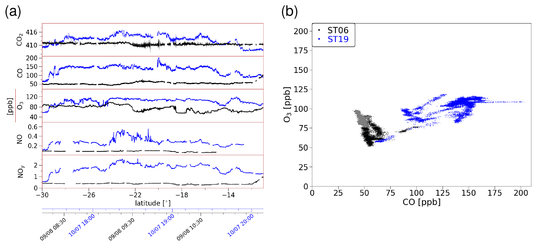
Figure 2 Latitudinal cross section for various chemical tracers measured during the transfer flights (a) from and to Buenos Aires (on 8 September 2019 (black) and four weeks later (7 October 2019, blue). The correlation between observed O₃ and CO mixing ratios is shown in (b). Grey dots mark mixing ratios of flight ST06 south of −22.75°.

Overall the data indicate, that strong pollution was encountered over this part of the flight as also pointed out by Johansson et al. (2022) who assume, that biomass burning contributed to a large extent to the observed tracer perturbations during flight ST19.

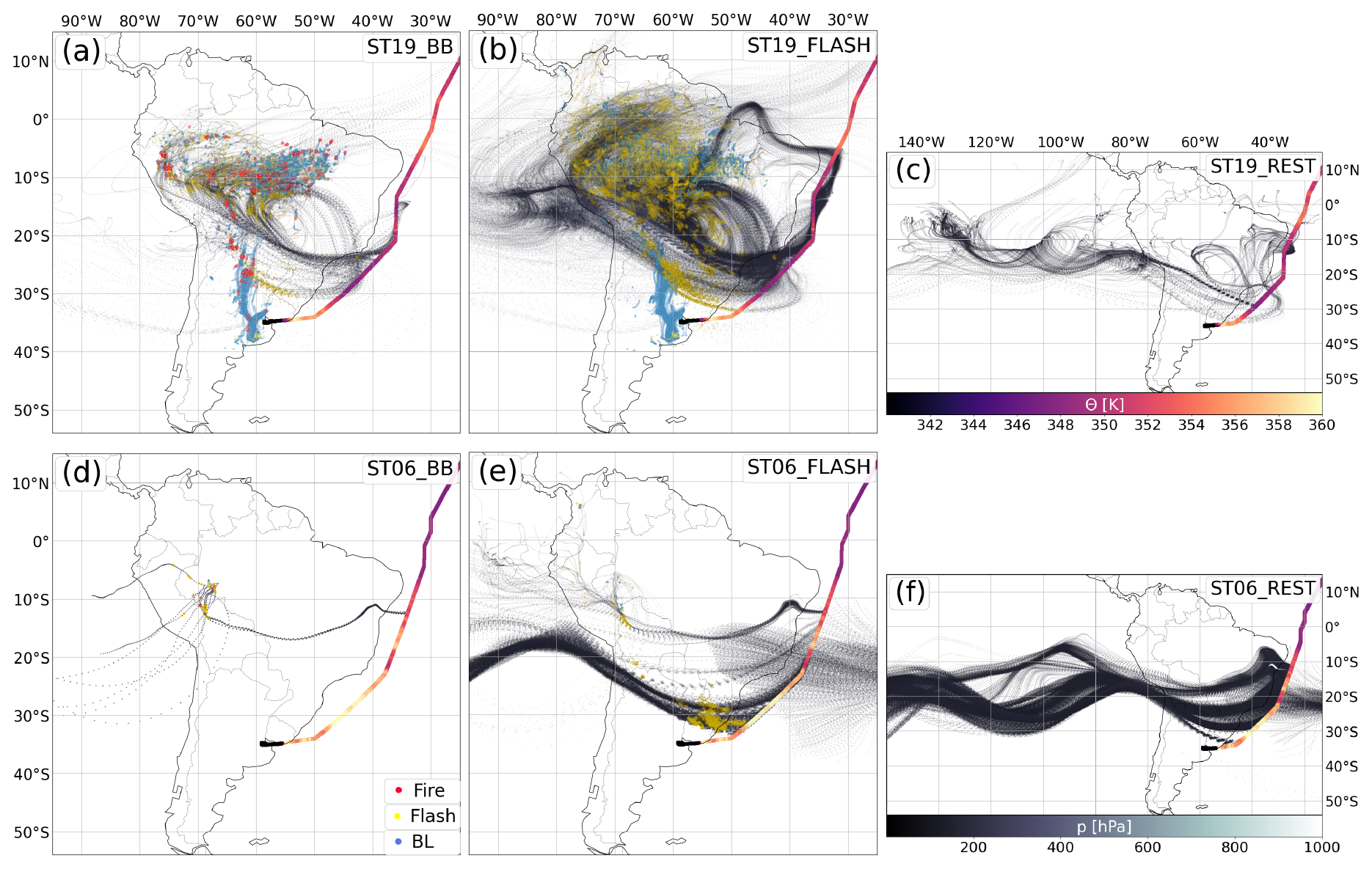
Figure 3 Plots show the pressure [hPa] (see colour code f) along all backward trajectories being started south of 10° S for flight ST19 (a, b, c) and ST06 (d, e, f) for each simulation scenario defined in Sect. 2.3.4, Table 1: BB (a, d), FLASH (BL + noB b, e), REST (c, f). Red circles mark the time of biomass burning emissions, yellow circles the time of LNO_x emissions and blue circles the time of boundary layer contact. Θ along the flight track is shown in all plots (see colour code c).

3.2 Synoptic conditions and trajectories

Potential vorticity level from ERA5 indicate that both flights in the considered latitude range took place in the upper subtropical troposphere at PV levels between PV = 0 and PV = −3.0 pvu. During the 7 d prior the flights, synoptic conditions over South America were significantly different. The South Atlantic subtropical high (SASH) was positioned relatively stable over the south-west Atlantic between 40–20° W and 40–20° S during the beginning of October 2019 (ST19) while at the beginning of September (ST06) a strong low pressure system passed southern South America and impacted the atmosphere up to latitudes north of 30° S. Therefore, the tropospheric outflow pattern is much more homogeneous in October compared to September. This is supported by a series of forward trajectories starting in six hourly time intervals at the surface over the Amazon Basin (in a square between 80, 50° W and 5, 15° S) on 1 September indicating very heterogenous transport pathways to the Atlantic over a broad altitude range.

GOES satellite data show a continuous band of high reaching clouds stretching from North-West Brazil to South-East Brasil the first days of October indicating, in combination with ERA5 surface charts, a well defined SACZ.

Figure 3 shows all simulated backward trajectories being initiated south of 5° S. A large number of ST19 trajectories descend into the atmospheric boundary layer crossing fires over South America (Fig. 3a) while this fraction is negligibly small for ST06 (Fig. 3d). The same holds generally for the number of boundary layer contacts over the South American continent which are less for ST06 compared to ST19 (Fig. 3a, b, d, e). Boundary layer contacts take predominantly place over rural regions with very small anthropogenic emissions but significant biogenic as well as biomass burning emissions.

Numerous trajectories cross lightning regions while being in the upper troposphere for both flights, however, the number of trajectories as well as the number of crossed lightning events is much larger for ST19 than for ST06 (Fig. 3a, b, d, e). It is also obvious, that flow patterns differ for both flights. BB and FLASH trajectories for ST19 circle over South America while they show predominantly a westerly flow for ST06.

On average, backward trajectories need ≈7 d to have boundary layer contact for both flights. In general, boundary layer trajectories are lifted rapidly into the upper troposphere after fires have been crossed even though they do not explicitly experience convection in a lagrangian transport model. Since solely the grid scale vertical velocity is considered to calculate vertical motion in MPTRAC, it is likely, that we rather underestimate than overestimate the number of uplifted BB trajectories. In addition, grid scale vertical transport usually takes place on longer timescales than convective uplift.

Generally, convective activity over South America is high in September and October as well as fire activity. The number of fire counts detected by the GOES fire detector does not differ significantly between ST19 and ST06. Neither does the average fire radiative power or the fire regions.

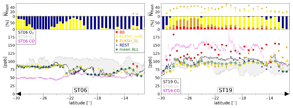
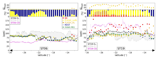
Figure 4 Plots show observed O₃ (black + grey line) and CO (purple line) mixing ratios along the flight track of ST06 (a) and ST19 (b). The grey shaded area indicates the differences in observed O₃ mixing ratios between flights ST06 and ST19. Coloured marks give the simulated trajectory mean of each simulation scenario (BB, FLASH_BL, FLASH_noBL, REST, see legend in a) and the mean of the entire trajectory ensembles (mean ALL) consisting of 240 trajectories starting every 5 min along the flight track. The bars give the fraction of trajectories belonging to each simulation scenario and yellow dots in the top row give the average number of lightning events for scenarios FLASH_BL and FLASH_noBL.

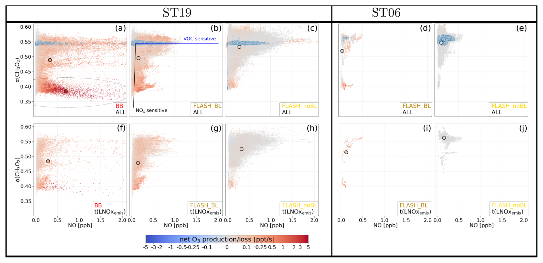
Figure 5 Simulated daytime O₃ as a function of NO mixing ratios and ${\mathit{\alpha }}_{\left({\mathrm{CH}}_{\mathrm{3}}{\mathrm{O}}_{\mathrm{2}}\right)}$ at all trajectory positions (a–e) and at the time of lightning emissions t(LNOx_emis) (f–j) for the simulation scenarios BB (a, f), FLASH_BL (b, g, d, i) and FLASH_noBL (c, h, e, j). Large circles with a black edge mark the mean of all trajectory points. Large circles with blue edges in the top row (a–e) mark the trajectory position at the flight track. Shown are only trajectory points with L(O₃) < −0.01 ppt s⁻¹ and P(O₃) > 0.01 ppt s⁻¹.

3.3 Chemistry

We focus our trace gas analysis on the latitude range between −30 and −11° S where HALO flew at a constant pressure level of 179 hPa (pv between 0 and −1 PVU) during ST19 related to O₃ mixing ratios of almost constantly 115 ppbv and CO mixing ratios of 150 ppbv. During ST06 the flight level increased from 161 hPa north of −22° S to 146 hPa further south. This ascent of the airplane is associated with an increase of O₃ mixing ratios to 80–100 ppbv which are south of −22° approximately the same order of magnitude as during ST19. The increase of O₃ is however related to a decrease in CO mixing ratios, a decrease towards stratospheric values of ERA5 pv level along the flight track from 0/−1 to −2/−3 and a descending vertical wind in the ERA5 data south of −22°. Therefore it is unlikely, that trace gas mixing ratios in this region are impacted by polluted boundary layer air masses (grey dots Fig. 2b). Absolute mixing ratios of CO are continuously smaller than O₃ mixing ratios in the considered latitude range for ST06 (vice versa for ST19) indicating unpolluted air in the upper troposphere and eventually stratospheric influence. The latter is however weak as O₃ mixing ratios increase between −22 and −30° but they are still below 100 ppbv. Clearly, air masses during both flights (ST06, ST19) represent significantly different atmospheric regimes (Fig. 2b).

To investigate the reason for the strong ST19 ozone enhancements in more detail and the chemical history of the air masses for both flights, we have applied the CAABA box model along all trajectories shown in Fig. 3. We compare the observations with the means of the entire trajectory ensembles (consisting of 240 trajectories, green circles Fig. 4) and the mean of each simulation scenario (listed in Table 1) having the same start time (i.e. 5 min time interval) at the flight track position.

Looking first at flight ST19, it is evident that O₃ mixing ratios of scenario BB (red squares, Fig. 4b) are much higher than for all other simulation scenarios and are much higher than the observations (black line). However, the simulated O₃ means of the entire trajectory ensemble (green circles, Fig. 4b) generally agree well with the measurements along the flight track, though the model slightly underestimates O₃ mixing ratios (green circles vs. black line, Fig. 4b).

Production of O₃ (P(O₃)) along the trajectories (before reaching the flight track) is clearly highest for BB trajectories at the time of BB emissions (large black ellipse, Fig. 5a) when both NO and VOC mixing ratios are high (${\mathit{\alpha }}_{\left({\mathrm{CH}}_{\mathrm{3}}{\mathrm{O}}_{\mathrm{2}}\right)}$ small). Furthermore, P(O₃) is enhanced at the time of LNO_x emissions, in particular for scenarios BB and FLASH_BL when air masses are in the upper troposphere but still carry sufficient amounts of VOCs emitted by either biomass burning (BB, Fig. 5f) or biogenic emissions (FLASH_BL, Fig. 5g, i). Production rates of O₃ are therefore higher for FLASH_BL (Fig. 5b, g) compared to FLASH_noBL trajectories (Fig. 5c, h) showing that the availability of VOCs in the upper troposphere controls O₃ formation in a VOC limited regime. Trajectories at the flight track position (blue circles, Fig. 5 upper row) are either in a VOC limited (high NO, high ${\mathit{\alpha }}_{\left({\mathrm{CH}}_{\mathrm{3}}{\mathrm{O}}_{\mathrm{2}}\right)}$) or transition regime (small NO, high ${\mathit{\alpha }}_{\left({\mathrm{CH}}_{\mathrm{3}}{\mathrm{O}}_{\mathrm{2}}\right)})$.

Mean O₃ mixing ratios at the flight track for FLASH trajectories (yellow stars, brown diamonds Fig. 4b) are almost always below observational values with an exception north of −14° S where in particular FLASH_BL trajectories show high (>100 ppb) O₃ mixig ratios. For these trajectories the residence time in the UT after the last boundary layer contact is on average 2 d longer than further south giving more time for more O₃ formation as VOCs are still sufficiently available in the air mass.

In the latitude range between −22 to −19° S, air mass history is different compared to the time before and after: Boundary layer contacts of the trajectories starting there, took place over south east South America (south of Buenos Aires, see cluster of blue dots in Fig. 3a, b)). Biogenic emissions from there are not as strong as from Amazonia (Sindelarova et al., 2014, Fig. 2a) explaining the small difference between scenarios FLASH_BL and FLASH_noBL. Simulated total VOC mixing ratios at the flight track are on average 15–20 ppb larger for scenario FLASH_BL compared to FLASH_noBL apart from the latitude range −22 to −19° S, where the difference is only in the range of 5 ppb. In this latitude range, O₃ production for both FLASH scenarios is predominantly driven by lightning NO_x emissions, O₃ mixing ratios of scenario FLASH_noBL (yellow stars) are even slightly higher than for scenario FLASH_BL (brown diamonds). However, there were fires over northern Argentina in regions where trajectories had BL contact, leading to high O₃ mixing ratios for scenario BB.

Simulated NO mixing ratios are on the same order of magnitude as observations, with a slight northward shift of an observed NO maximum along the flight track between −20 and −24° S (Figs. S2 and 2a). The amount of emitted NO per flash underlays a large uncertainty. In a sensitivity simulation (not shown here), we enhanced LNO_x emissions by a factor two. This leads to a tremendous overestimation of NO mixing ratios compared to the flight observations. Even with these unrealistically high NO mixing ratios, P(O₃) does not increase significantly in scenario FLASH_noBL as air masses in the regions of lightning are mainly in a VOC sensitive regime (Fig. 5h).

It is likely that the impact of surface emissions in general, especially local emission maxima are underestimated in the EMAC simulation used for initial and boundary conditions (mixing of air mass in the CAABA box with “ambient air”) as the EMAC grid is rather coarse, i.e., a spectral resolution of T42 (≈2.8°). Additionally, we might miss fires when they are close to but not exactly at the trajectory position. Furthermore, the time of LNO_x emissions in CAABA is based on satellite data which are independent of ERA5 data driving the MPTRAC trajectories. Therefore, convective activity in ERA5 is rather small at some locations where GOES detects lightning events which are most likely connected to an uplift of boundary layer air masses into the UT. In addition, it is possible, that we generally underestimate the number of BL trajectories as mentioned in Sect. 3.2.

Therefore, we performed a set of CAABA simulations (CAPE_high) for ST19, doubling EMAC (“ambient”) VOC mixing ratios at trajectory locations, where CAPE in ERA5 is greater than 1000 J kg⁻¹ and flashes were observed but trajectories had no BL contact before (scenario FLASH_noBL). Thus, the more such events are found along a trajectory, the higher VOC mixing ratios get due to mixing of the air within the CAABA box with VOC enriched “ambient” EMAC air compared to our base simulation.

Indeed P(O₃) along these FLASH_noBL trajectories gets larger (Supplement, Fig. S3a, yellow stars) which also leads to higher ensemble means of O₃ mixing ratios, in particular between −24 and −18° S (Supplement, Fig. S3a, green circles) agreeing now very well with the observations.

For ST06, simulated O₃ mixing ratios (Fig. 4a, green circles vs. black line) agree very well with the observations. CAABA simulations only show a southward shift of the local O₃ maximum at $\approx -\mathrm{19}$° S. The fact that the number of BL contacts for ST06 trajectories is negligibly small (or zero), related to small upper tropospheric mixing ratios of VOCs and NO_x explains the much smaller O₃ mixing ratios during ST06 (especially north of −22°) compared to ST19. In the latitude range between −24 and −20° S, the majority of trajectories cross lightning regions (detected by GOES) however, the number of flashes per trajectory is on average much small than for ST19 trajectories (top row, Fig. 4a, b). Again, CAABA air masses are in a VOC sensitive or transition regime at the time of LNO_x emissions (Fig. 5i, j) thus adding more NO_x would not lead to a higher O₃ production.

In contrast to ST19, simulated mean O₃ mixing ratios for ST06 agree well with observations without the injection of additional VOCs. Lightning events in ST06 (between −24 and −20°) are close to the flight track over coastal regions. It is likely that air masses which are lifted convectively there (in the vicinity of lightning) carry rather clean (marine) air into the UT rather than polluted air explaining the good agreement even though MPTRAC trajectories have no BL contacts at all.

Simulated O₃, VOC and NO_x mixing ratios for FLASH_noBL scenarios are higher (Figs. 4, 5h, j) for ST19 compared to ST06 even though for both flights these trajectories remain in the upper troposphere at similar pressure levels throughout the backward simulation time. This difference can be explained, as all trajectories are initiated and nudged with EMAC data representing the background atmosphere which is saturated with fire emitted species in October. Thus, all trajectories are exposed to these background air masses, also those of scenarios REST and FLASH_noBL. Therefore, we performed another set of CAABA simulations (EMAC_noBB) for flight ST19 based on an EMAC simulation in which biomass burning emissions were switched off. This leads to O₃ mixing ratios which are ≈10 ppb smaller than in our base simulation (Supplement, Fig. S3b).

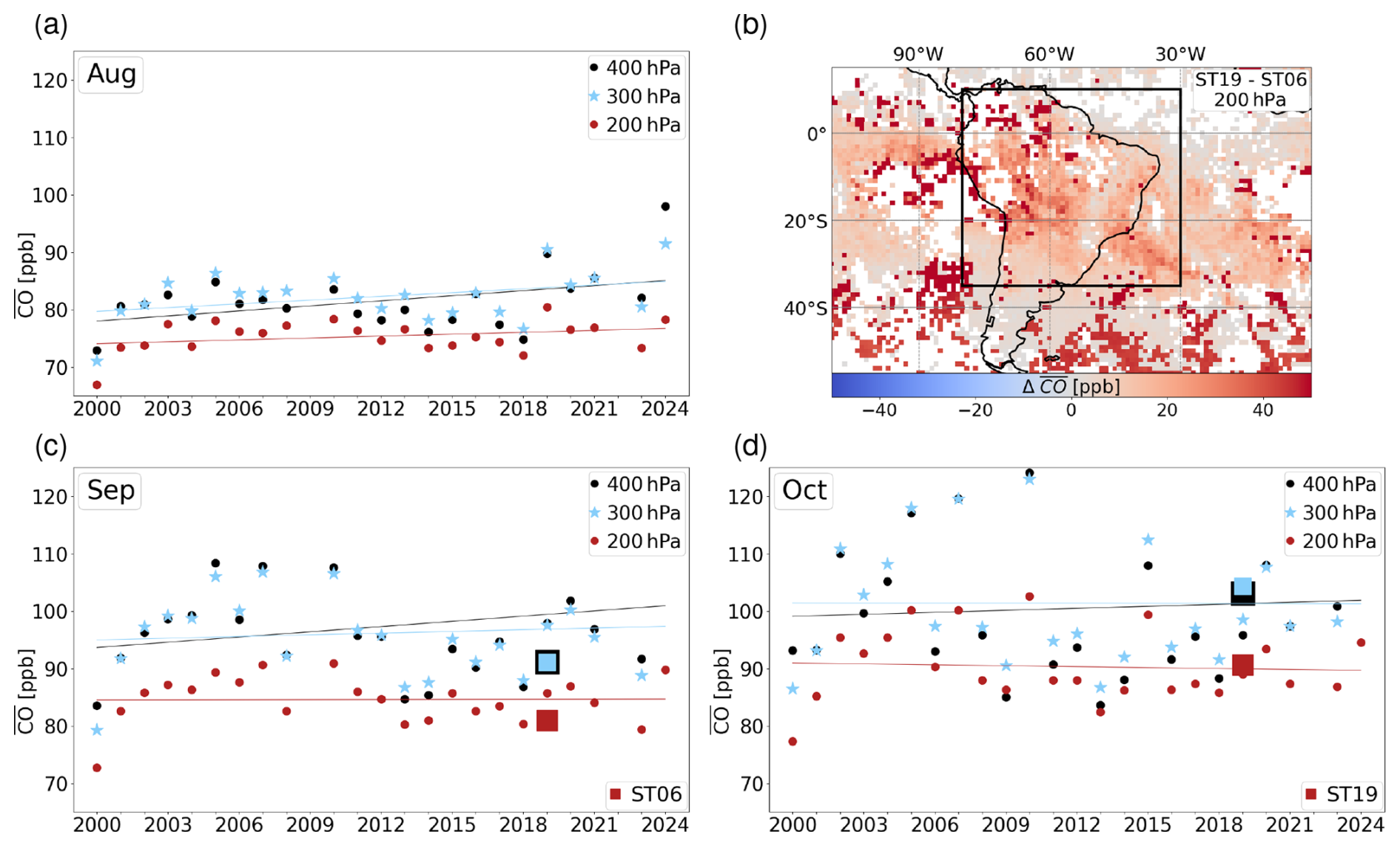
Figure 6 Shown (b) is the differences in CO mixing ratios derived from the MOPITT satellite instrument for the 10 d prior flight ST06 (29 August–8 September 2019) and ST19 (28 September–7 October 2019). Panels (a), (c), (d) show a climatology of CO monthly mean mixing ratios from MOPITT over South America (square in b) at 400 hPa (black), 300 hPa (blue) and 200 hPa (red). Squares show the 10 d CO mean prior flights ST06 (c) and ST19 (d).

3.4 CO Satellite data

To address the question of the representativeness of the SOUTHTRAC observations, we compare long term MOPITT satellite observations with observed CO mixing ratios. Comparing the 10 d mean of MOPITT CO mixing ratios prior the flight days (the trajectory backward simulation time), CO is significantly higher at 400, 300 as well as 200 hPa for ST19 compared to ST06 (Fig. 6b). This is generally not surprising since flight ST06 took place in the beginning of the South American biomass burning season and flight ST19 in the mid/end of the burning season.

Clearly visible are higher CO mixing ratios throughout the upper troposphere in October compared to August (Fig. 6a, d). The 10 d CO mean values for flight ST06 are close to the regression line of the climatology for September for all three shown pressure level (Fig. 6c).

For ST19, the 10 d mean at 200 hPa agrees also well with the climatological mean while values at 300 and 400 hPa are slightly above the mean (also the 2019 October mean, (Fig. 6d)). However, CO mixing ratios at these pressure levels have a much larger inter-annual variability in October compared to August and September. Therefore, we can conclude that conditions before/during both flights are not exceptional but rather typical of the time of year (i.e. beginning of September and October) and region.

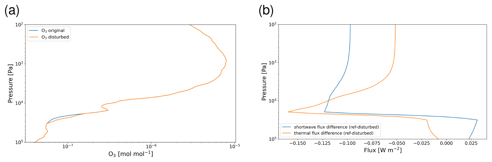
Figure 7 Estimated effect of the ozone perturbation (left) as observed during ST06 and ST19 on the radiative fluxes in the UTLS (right) showing a reduction of the upward shortwave radiative fluxes of 0.1 W m⁻² at the top of the atmosphere.

3.5 Consequences for the radiation budget

To estimate the effect of the perturbed ozone on the radiation budget, we applied a modification of the ozone profile in the UTLS as observed during the flights to the simulated background ozone field. We used a 1D-column model with the same radiative code as in the global EMAC model as described above (Dietmüller et al., 2016). The vertical profiles for the other radiatively active compounds have been extracted as mean values for the respective region from a global chemistry-climate model simulation with EMAC. Effects of aerosols have been neglected, as the focus is solely on the radiative effect of the O₃ enhancement. As shown in Fig. 7 we find a reduction of both, shortwave and longwave fluxes in the stratosphere which peaks in the UTLS. It reduces radiation from the troposphere and therefore reduces absorption in the stratosphere. The sum of both longwave and shortwave reduction near the tropopause is on the order of 0.25 W m⁻². As expected the enhanced ozone at the cold tropopause leads to upward LW-fluxes which are smaller compared to the unperturbed case. The effect is at maximum at the tropopause and reduces towards the surface. The upwards oriented shortwave flux reduction is on the order of 0.1 W m⁻² at the top of the atmosphere which is enhanced by a longwave effect of 0.05 W m⁻², resulting in an total TOA effect of 0.15 W m⁻². Near the surface a slight increase in shortwave radiation is compensated by a similar longwave cooling. Notably, this only reflects the impact of ozone without accounting for aerosols or water vapour co-emitted by the fires. The numbers are in line with estimates of the radiative kernel by (Rap et al., 2015) who found sensitivities of approximately 3–5 mW m⁻² ppbv⁻¹ per 100 hPa, which would correspond to 90–150 mW m⁻² net flux disturbance for an ozone perturbation of 30 ppbv in a layer of 100 hPa (compare Fig. 2).

4 Discussion

Based on our CAABA simulations, we can conclude that solely in the presence of sufficiently high VOC and NO_x mixing ratios, the observed amount of ST19_O₃ can be produced and that required VOC mixing ratios are of orders of magnitude needing a very strong emission source. As mentioned in Sect. 3.2, ST19 trajectories have almost solely BL contact in rain forest or rural regions, where anthropogenic emissions are small but biomass burning emissions are high. Biogenic emissions provide as well a VOC source required for UT O₃ production as the results of our simulation scenario FLASH_BL and our CAPE_high experiment show. Even though it is possible, rather likely that we underestimate the impact of biomass burning emissions in total we can conclude, that biomass burning VOC emissions are necessarily required for reproducing the observed O₃ mixing ratios, in particular by comparing our base simulation setup and our EMAC_noBB experiment. Regarding CO mixing ratios in the upper troposphere, they show a distinct annual cycle with largest values at the end of austral spring (i.e. October) and smallest values between April and June. The layer of enhanced CO mixing ratios in October can be seen in the MOPITT satellite dataset in the entire upper troposphere up to 200 hPa. Biogenic emissions contribute all year round to the atmospheric composition, though they are smallest in the South American dry season (July–October) and highest in the wet season (December–March) (Sindelarova et al., 2014). Thus their maximum is opposite to the upper tropospheric CO maximum. CO mixing ratios are highest in September and October, i.e. the time of year with highest biomass burning emissions. Therefore, our observed CO level and their agreement with climatological values give a further indication, that the observations made during flight ST19 are heavily impacted by biomass burning.

A study by Tripathi et al. (2025) concludes, that convective uplift of soelely biogenic emissions leads to the production of elevated O₃ level observed by them in the UT over the South American continent. Though, the observations analysed by Tripathi et al. (2025) were made from December to January, thus at the beginning of the South American wet season where biogenic emissions are significantly larger than during the time of our measurement flights.

Considering the ratio between observed CO₂ and CO mixing ratios, it is distinctly different for flights ST06 (both species are negatively correlated with a slope of the regression line of $m=-\mathrm{7.8}$, $r^{\mathrm{2}}=-\mathrm{0.65}$) and ST19 (m=8.65, r²=0.9). Other studies report slopes of m=0.057 (Mauzerall et al., 1998) and m=40 (Hooghiem et al., 2020) for biomass burning plumes. The ranges of slopes of the regression line between CO₂ and CO is obviously very large. However, in case of a biomass burning impact, the slope is positive (like for ST19).

Dickerson (1984) present NO observations taken along the Brazilian coast in December 1983 on board of a commercial aircraft along a similar flight track as for flights ST06 and ST19. They observed smaller mixing ratios of NO in the Northern Hemisphere (≈0–30 ppt) compared to the Southern Hemisphere (≈50–150 ppt, in the latitude range between −25 and 0° S) and attribute this difference to enhanced lightning activity over the South American continent and assume that biomass burning does not play a role for upper tropospheric NO level in December. If this is true, the difference in their observations and our observed NO mixing ratios, being at the same locations more than a factor two higher than reported by Dickerson (1984) provides a further indication that our observations are strongly impacted by biomass burning, especially as biogenic emissions should be higher in December compared to October.

Our results clearly reveal, that LNO_x emissions alone cannot be responsible for the formation of the observed O₃ level during flight ST19. This is in contrast to the assumption by Sauvage et al. (2007) and Jenkins et al. (2021) who assume that lightning produced NO_x dominates O₃ formation in the upper troposphere above 500 hPa causing subsequently the South Atlantic O₃ maximum. Our findings regarding the O₃ formation processes is in agreement with the study by Bozem et al. (2017) who conclude that due to convective uplift of precursor gases such as HCHO and H₂O₂, HO₂ mixing ratios can be enhanced in the upper troposphere facilitating O₃ formation. They are also in agreement with an early study of Pickering et al. (1996) who link enhanced UT O₃ levels observed in aircraft data and O₃ soundings from Natal (northeast Brazil coast site) with biomass burning over central Brazil and deep convective transport of these emissions accompanied by a contribution from lightning. Pickering et al. (1996) calculated a net O₃ production of 5–6 DU (≈167–201 [molec. cm⁻³] $\times {\mathrm{10}}^{-\mathrm{9}}$) over 8 d after the convective event integrated over the outflow layer between 8 and 16 km altitude. Our simulated 7 d integrated net O₃ production is comparable to the values given by them, though our simulations show a larger mean value of 304 [molec. cm⁻³] $\times {\mathrm{10}}^{-\mathrm{9}}$.

Most studies analysing O₃ production regimes focus on the boundary layer or lower troposphere often with the purpose to quantify the impact of different emission sources on O₃ production which enables the development for mitigation strategies to diminish air pollution. Few studies investigate NO_x and VOC related O₃ production regimes in the upper troposphere. Based on their modelling study using the EMAC model, Nussbaumer et al. (2023) conclude, that in the ITCZ over continental areas, in particular Africa and South America, ozone chemistry is mostly VOC sensitive or in the transition regime which is in agreement with our findings for the UT over South America. Following the discussion in Nussbaumer et al. (2023), older studies assuming an upper tropospheric NO_x sensitive O₃ regime over the US and the North Atlantic based on aircraft observations (Jaeglé et al., 1998; Wennberg et al., 1998; Jaeglé et al., 1999) presumably overestimated the reaction between NO₂ and OH as it is known today that the reaction rate of NO₂ and OH is much lower than previously assumed. An early study by Pickering et al. (1990) reported a VOC-sensitive regime over the USA at 11 km altitude based on measurements in June 1985 and model simulations. A more recent study by Tripathi et al. (2025) also comes to the conclusion, that O₃ formation in a NO_x rich upper troposphere (due to lightning) is limited by the abundance of VOCs. However, Tripathi et al. (2025) also use the EMAC model in a similar configuration as we do. Thus it is likely that both studies reveal the same conclusions.

A study by Tsivlidou et al. (2023) presents a seasonal O₃ climatology based on IASI and IAGOS data showing an O₃ and CO maximum over the Southwestern Atlantic and over Brazil for October. A distinct O₃ maximum is also visible over the Southwestern Atlantic in January but at this time of the year to a lesser extent over the South American continent while CO mixing ratios are much smaller in January than in October.

Combining our results with the results by Tripathi et al. (2025), we hypothesise, that the winter (January) O₃ maximum is driven mainly by biogenic (VOC) emissions and subsequent convective uplift and photchemical processing while we can clearly state that the autumn (September, October) O₃ maximum is dominated by fire emissions and subsequent chemical processing.

5 Conclusions

Two transect flights during the SOUTHTRAC mission under pristine and highly polluted conditions in the UTLS provide a unique dataset to assess the combined impact of biomass burning as well as biogenic emissions in addition to lightning NO_x emissions on the upper tropospheric composition. To our knowledge, the in-situ observation of a southern hemispheric upper tropospheric O₃ maximum extending several hundred kilometers from −11 to −30° is very rarely (if at all) reported before, in particular not at a pressure range between 146 and 179 hPa.

Based on our analysis combining Lagrangian box model simulations, satellite derived biomass burning and lightning activity, ERA5 reanalysis data and EMAC model data as well as MOPITT satellite data, we could directly link our observation to a detailed analysis of the driving processes relevant for ozone production. We could show, that surface emissions of VOC from biogenic sources and biomass burning are essential to explain the observed UT ozone maximum and that the convective uplift of VOCs is a key mechanism for the production of ozone in the UT. Though we use state of the art emission data sets some uncertainties remain in the correct emissions and thus the associated impact. Similarly the representation of convection in ERA5 is limited. The fractional contribution of biomass burning or LNO_x induced O₃ production is however, difficult to determine. Both source processes underlay a very high variability in space, time and in strength and have generally an uncertainty in their model representation. However, since our study shows a continental scale impact rather than individual small scale plumes the aforementioned limitations are partly compensated for. We therefore conclude that the observed enhanced O₃ level of ≈120 ppbv in the outflow region east of the South American continent are the combined result of VOC emissions and lightning during convective uplift. This is in agreement with the findings of an early study by Pickering et al. (1996). We extend previous findings by directly linking surface and lightning NO_x emissions with O₃ production regimes. To analyze the chemical regimes we combined our Lagrangian chemical box model approach with a recently developed method by Nussbaumer et al. (2023), which has been shown to be well suited for typical atmospheric conditions in the upper troposphere.

We show, that the availability of upper tropospheric VOCs emitted both by biomass burning as well as biogenic processes in the presence of lightning NO_x control O₃ production in the UT approximately 5 to 7 d after emission and that the chemical composition of the South American UT outflow is associated with strong uplift by convection over South America, mostly over the pristine rain forest of Amazonia. Lightning NO_x emissions certainly contribute to the upper tropospheric O₃ production but they alone are not sufficient to produce the observed mixing ratios neither of O₃ nor NO. The fractional contribution of biomass burning or LNO_x induced O₃ production is however, difficult to determine. Both source processes underlay a very high variability in space, time and in strength and have generally an uncertainty in their model representation.

The simulated radiative effect of the enhanced upper tropospheric O₃ layer of 0.15 W m⁻² at the top of the atmosphere can be considered as significant and is in the same order of magnitude as the shortwave direct aerosol radiative effect induced by African biomass burning aerosol transported over the South East Atlantic (clear sky effect: −0.09 W m⁻² yr⁻¹, all sky: 0.04 W, Jouan and Myhre, 2024).