Radar data shows graupel and increased turbulence near small-scale intermittent lightning discharges at the top of intense thunderstorms

Sparkles are the intermittent, small-scale lightning discharges that occur near the top of intense thunderstorms. To increase the understanding of mechanisms that lead to sparkles, we compare high resolution lightning data from the LOw Frequency ARray (LOFAR) to data from a meteorological radar. The study focuses on the thunderstorms that crossed the northeast of the Netherlands on 18 June 2021. We use a two-stage clustering approach to computationally distinguish sparkles, defined as small and isolated lightning structures, from other lightning activity. Subsequently, we compare the radar data near sparkles to radar data near the other lightning activity. From radar images, we conclude that the convective systems that produced sparkles exhibit supercellular characteristics. Consistent with previous studies, we find that sparkles were present at high altitudes when radar reflectivity values were relatively high. Such values are associated with strong updrafts, lofting of graupel, and overshooting cloud tops. We confirm with a fuzzy-logic hydrometeor classification algorithm that graupel is often present near sparkles. Near sparkles, radar data also shows enhanced spectral width values and heterogeneous patterns in the radial velocity. This likely represents enhanced turbulence. Our observations match hypotheses to explain the small extent of sparkles, namely folding of a charged screening layer, and fragmentation of existing charge pockets. Additionally, we hypothesize that inductive charging, enhanced by turbulence, could play a role in the formation of sparkles.

1 Introduction

The LOw Frequency ARray (LOFAR) is a radio telescope that is in use for astronomical observations and consists of numerous radio antenna fields, of which the core is situated in the northernmost part of The Netherlands (van Haarlem et al., 2013). Previous studies have shown that LOFAR antennas can detect electromagnetic signals from lightning. By correlating the observations at the various antenna fields, 4-dimensional (spatial and temporal), high-resolution images can be constructed of point sources in the VHF (Very High Frequency) radio band (Hare et al., 2018). This methodology has been exploited to study a large variety of lightning structures with much detail (Hare et al., 2019; Scholten et al., 2021c, a, b; Liu et al., 2022; Scholten et al., 2023).

In order to introduce the LOFAR lightning images and to illustrate some of the visible lightning structures, Fig. 1 shows part of the LOFAR image at 19:54:22 UTC on 18 June 2021. Annotations with numbering 1 through 4 show some exemplary lightning structures. Annotations 1, 2 and 4 mark negative stepped leaders (Mazur, 2016). For structures 2 and 4, the propagation at the end of structure 2 and 4 is clearly visible as slanted lines in Fig. 1a. Annotation 1 marks a negative leader that is mostly propagating horizontally. As is common for negative leaders at high altitudes, it propagates relatively slow (Scholten et al., 2021a). Dart leaders live on previously established leader channels and therefore propagate much faster than negative stepped leaders (Mazur, 2016). They show up as nearly vertical lines in Fig. 1a. Annotation 3 marks one of the many dart leaders in this LOFAR image. At ∼ 350 ms, a dart leader is also visible on the channel of structure 1. Positive leader propagation is not well captured by LOFAR. However, after the positive leader channels have been established, other lightning activity in the same channel can reveal its location. Hare et al. (2019) use, for example, dart leaders and needle activity to locate positive leader channels. In Fig. 1 there is no obvious signs of positive leader channels. However, there is a layer between ∼ 7 to ∼ 9 km altitude, that is almost devoid of negative leaders. Negative leaders propagate away from this layer. We therefore infer that this layer was negatively charged. The positive leaders which are expected to balance the negative leader growth, were likely present in the negatively charged layer.

Figure 1 Part of the LOFAR image at 19:54:24 UTC on 18 June 2021. The dots show VHF point sources from lightning. The color of the VHF sources mark the timing with respect to the start of the LOFAR image. Panel (a) shows the altitude vs the timing. The bottom three panels show the projection of the VHF sources on to the planes of a three-dimensional box, a horizontal plane in panel (c) and two adjacent vertical planes in panels (b) and (d). Annotation 1, 2 and 4: Negative stepped leaders. Annotation 3: A dart leader. Sparkles are observed as a cloud of small, intermittent discharges above 8 km altitude.

Besides the large lightning structures, Fig. 1 also shows many VHF sources that seem disconnected in time and space. These small lightning structures were mainly present above an altitude of 8 km and up to almost 14 km. In LOFAR images, the altitudes above 10 km are usually not much populated. However, for the thunderstorms on 18 June 2021, the “cloud” of the small-scale, intermittent VHF sources persisted over multiple LOFAR images, spanning more than an hour. The observations of these small-scale, high-altitude, intermittent discharges have been described in Scholten et al. (2023) and are named “sparkles”. In the same study, the authors show that sparkles have specific spatio-temporal structures. Some of the sparkles behave in a similar manner as negative stepped leaders and even exhibit dart leaders.

At first glance, sparkles and needles (Hare et al., 2019) appear very similar in the LOFAR data: both are very small and temporally intermittent. However, needles are attached to larger lightning channels, whereas sparkles occur independently. In this work, we focus only on sparkles.

Numerous studies of thunderstorms in the United States report similar observations to sparkles (Lhermitte and Krehbiel, 1979; Bruning et al., 2010; Ushio et al., 2003; Calhoun et al., 2013; Emersic et al., 2011). Lhermitte and Krehbiel (1979) already showed in 1979 that an umbrella of sources can form above strong updrafts. Bruning et al. (2010) show that such umbrellas develop simultaneously with updraft surges. They hypothesize that the small discharges in above the updrafts are either related to turbulence, sweeping out patches of charge from the updraft, or the heterogeneous circumstances and complex 3-dimensional flow at the cloud tops. Calhoun et al. (2013), Emersic et al. (2011) and MacGorman et al. (2017) hypothesize about small discharges between the charged updraft and an oppositely charged screening layer around the cloud. Periodic folding of the charged screening layer due to turbulence, would be the mechanism to bring the two sources of opposite charge together, close enough for dielectric breakdown. Calhoun et al. (2013) also hypothesize that these small discharges live in small charge pockets that limits their spatial extent. Simulations by Calhoun et al. (2014) show that charge pockets may result from turbulent mixing of a heterogeneously charged updraft. Brothers et al. (2018) give convincing evidence with their simulations that in updraft columns, turbulence can produce many small charge pockets. The sub-kilometer size of these charge pockets do match the spatial scales of sparkles.

Despite these previous studies, there is no conclusive theory about the mechanisms that cause sparkles. By combing the LOFAR data with radar data, it is the aim of this study to advance the knowledge of small-scale, intermittent discharges.

We compared the LOFAR data of the 18 June 2021 thunderstorms with data from a polarimetric (dual-polarization) meteorological radar, located on Borkum Island, Germany. Scanning the atmospheric volume, the outgoing beam reflects upon hydrometeors (water particles or drops) or other particles to give a backscatter signal. The Doppler shift of the signal provides insight into the velocity spectrum of hydrometeors (Doviak et al., 1993). The different polarimetric variables can be used to deduce the location, abundance, and the type of hydrometeor (Doviak et al., 1993; Marzano et al., 2006). With this information, it is possible to characterize storms and locate dynamical aspects such as updrafts and downdrafts (Kumjian, 2013a, b).

To gain insights in the atmospheric conditions in the vicinity of lightning, and sparkles in particular, a two-stage clustering technique is employed to find the time and locations of sparkles occurrences in the LOFAR data. The location information is used to populate statistics on radar polarimetric variables, both for (1) sparkles and (2) other lightning discharges present in the LOFAR data. These two statistical groups are subsequently compared. The results of this case study are also qualitatively compared with previous studies by Bruning et al. (2010), Emersic et al. (2011), Calhoun et al. (2013) and MacGorman et al. (2017), and the aforementioned hypotheses.

The remainder of this paper is organized as follows. Section 2 describes key aspects of the methods used in the analysis. A detailed description of the methods can be found in the Appendices. Section 3 presents the data in this study in four parts: Sect. 3.2 provides an analysis of the storm evolution and different convective systems that are observed, Sect. 3.1 presents the LOFAR data, Sect. 3.3 presents the correlations found between radar and LOFAR data, and Sect. 3.4 notes key observations, alongside exemplary figures, from visual analysis of the radar images in the context of LOFAR data. Section 4 is dedicated to the interpretation and appreciation of the results. Finally, conclusions are provided in Sect. 5.

2 Methods

2.1 LOFAR

During thunderstorms, LOFAR dumps about 2 s of raw-voltage (transient buffer) data from 6 low-band antennas (LBA) per station, from 38 Dutch stations. This data dumping takes about 15–30 min, thus LOFAR can record up to 10 flashes per storm. The LBAs are inverted V dipoles that are sensitive to 10–90 MHz. After recording, the data is processed into images with the “impulsive imager”. This is an advanced time-of-arrival algorithm inspired by Kalman filters using cross-correlations to measure time-delays of pulses received by different antennas (Hare et al., 2018; Scholten et al., 2021d). The impulsive imager produces about 200 sources per ms with meter and nanosecond level accuracy.

2.2 Selecting Sparkles

Scholten et al. (2023) define sparkles as “spatially small (not exceeding a few 100 m) intermittent discharges near the top of the clouds where this activity is seen over extended periods lasting the full duration of a LOFAR recording.” An example of a LOFAR image with sparkles is given in Sect. 3.1.

In order to perform a quantitative analysis, we distinguish sparkles from other lightning structures using a two-stage approach. Inspired by Fuchs et al. (2016), we apply the DBSCAN (Density Based Spatial Clustering with Noise) algorithm as implemented in Scikit-Learn (Pedregosa et al., 2011) to group VHF sources into four-dimensional lighting structures. We used visual inspection and a trial-and-error approach to find appropriate normalization constants for clustering. The normalization constants determines if two VHF sources are far apart (larger than the normalization constants) or near each other (smaller than the normalization constants). The final parameters for the two-stage clustering approach are given in Table 1.

Table 1 Relevant parameters for clustering approach.

In the first stage, we normalize the time and spatial coordinates of all VHF sources by dividing by normalization constants of 0.3 s and 2 km respectively. We then run DBSCAN with a minimum cluster size of 30 points, classifying each resulting cluster as “other VHF sources”. Unclustered points, which are apparently not part of any large cluster, proceed to the second stage.

In the second stage, we re-normalize the original time and space by dividing by 0.02 s and 200 m respectively, and now use DBSCAN with a minimum cluster size of 2 points. These clusters are classified as sparkles. Any remaining VHF sources, which were thus potentially part of sparsely imaged large clusters, are added to the “other VHF sources” category.

Finally, we reassign any sparkle VHF source to the “other VHF source” category if it is located below an altitude threshold of 8 km. This threshold removes a small number of outliers below this threshold.

The result of the sparkle classification algorithm as described above, is a categorization of each LOFAR VHF source as either a “sparkle”, or as an “other VHF source”.

By design, the VHF sources that are marked as sparkles only entail relatively small isolated clusters. It is likely that needles, which connect to decaying positive leader channels, are not classified as sparkles.

2.3 Polarimetric Radar Data

The radar data that is used in this study comes from a polarimetric C-band radar, located on the island of Borkum in Germany. This specific radar was chosen given its favorable location and range with respect to the location of interest, i.e. the north of the Netherlands. The technical details of this radar can be found in Frech et al. (2017). The key aspects of the Borkum radar and data can be found in Appendix A.

2.3.1 Radar variables

In this study we use the following three radar variables: radar reflectivity (Z_h), radial velocity (V_rad), and velocity spectrum width (W_rad). Polarimetric variables are used in a hydrometeor classification (HMC) scheme to derive information about particle types in the radar measurement volume. The HMC scheme is discussed in Sect. 2.3.2. A brief description of Z_h, V_rad and W_rad follows, but the reader is referred to Doviak et al. (1993) or Kumjian (2013a) and Kumjian (2013b) for a more thorough description.

The radar reflectivity Z_h represents the power of the radar beam that is scattered back to the radar with horizontal polarization. In this study, we do not consider the vertically polarized reflectivity Z_v. Generally, the Z_h values for a radar resolution volume are higher when there are more hydrometeors, larger hydrometeors, or hydrometeors that have a larger fraction of water with respect to ice. The shape and orientation of hydrometeors is important for the ratio between Z_h and Z_v.

The radial velocity V_rad is computed from the Doppler shift of the backscattered signal. It represents the velocity of the hydrometeors in the outward radial direction. Note that V_rad is the reflectivity-weighted mean of the velocities of all hydrometeors within a radar resolution volume (Doviak et al., 1993).

The velocity spectrum width W_rad represents the spread in V_rad within a radar resolution volume and is computed as the reflectivity-weighted standard deviation of V_rad (Doviak et al., 1993). Either gradients in the velocity field, potentially in the form of turbulence, or presence multiple hydrometeors with different terminal sedimentation velocities, will lead to increased W_rad values.

2.3.2 Hydrometeor Classification

For radar data points, the type of dominant hydrometeor is estimated using the wradlib (Heistermann et al., 2013) fuzzy-logic hydrometeor classification (HMC) algorithm based on the method of Zrnić et al. (2001). As input, this algorithm uses polarimetric radar variables, and the conditional two-dimensional probability density functions of the following hydrometeor classifications: No Precipitation (NP), Vertically-aligned ice Crystals (VC), Horizontally-aligned ice Crystal (HC), Wet Snow (WS), Dry Snow (DS), Graupel/Hail (GH), Rain/Hail (RH), Hail (HL), Large Drops (LD), Heavy Rain (HR), Medium Rain (MR), and Light Rain (LR). The output is, per radar resolution volume and per hydrometeor type, the probability that this type of hydrometeor can explain the polarimetric radar variables. More details on HMC methods are described by Al-Sakka et al. (2013)

We classify the hydrometeor type with the highest probability as the dominant hydrometeor type for each radar point. Furthermore, the probability differences between different hydrometeor types can be used as an indication of the uncertainty of the HMC output. The radar variables considered for the HMC algorithm in this study are Z_h, differential reflectivity Z_dr, co-polar correlation coefficient ρ_hv and specific differential phase K_dp. The computation of the latter is described in Appendix B. In addition, we make use of ERA5 model data for temperature T. All variables are weighted equally. The conditional two-dimensional probability density functions (membership functions) are retrieved from (wradlib) (2024), which are constructed based on radar signal simulations by Marzano et al. (2006).

Throughout this work, we use the term “graupel” for the graupel/hail HMC category. Since we only consider radar data above 8 km altitude, with temperatures well below freezing level, the presence of graupel is more likely than hail. For this reason, we also assume that the graupel/hail HMC category mainly identifies graupel.

2.4 Matching radar with LOFAR data

Throughout the analysis, the LOFAR data is compared spatially with radar data. This process involves a standard correction for the refractive index of the atmosphere (Doviak et al., 1993), georeferencing and advecting the radar data according to the ambient wind velocity. These steps are elaborated on in Appendix B. Note that all radar images in this work are advected to the time as indicated in the figure caption.

In this study, we compare radar data within a 2 km radius of VHF sources identified as sparkles (Sect. 2.2) with radar data near other VHF sources. The latter category is radar data found within a vertical column of 2 km radius of other VHF sources, but not within a 2 km radius of sparkles. A minimum altitude threshold of 8 km ensures a fair comparison of radar variables, without any potential altitude bias. A Z_h>0 dB threshold ensures that we only use radar data with significant amounts of hydrometeors. Furthermore, the 0 dB threshold ensures that the signal is significantly above the noise level. Thus we do not consider the atmosphere outside clouds and clouds that are barely reflective to the Borkum radar.

We acknowledge that there may be errors in the advection of radar data (see Appendix B). Additionally, the coarse cross-beam radar resolution may obscure vertical gradients and therefore potentially bias the radar statistics. For some VHF sources more than 100 km away from the radar, the vertical radar resolution amounts to ∼ 4 km. In this light, it is a deliberate choice to take a 2 km radius to select radar data near VHF sources. At the same time, this coarse radius allows us to collect enough statistics. In a sensitivity analysis (not shown), changing the radius to 1 to 3 km did not lead to notably different results.

2.5 Statistical comparison

We compare the distributions of Z_h and W_rad values measured near sparkles with those measured near other VHF sources. To quantify differences between distributions we compute the two-sample Kolmogorov–Smirnov (KS) statistic and its p-value (Gideon and Mueller, 1978), together with Cliff’s delta as an effect size (Meissel and Yao, 2024). The KS statistic measures the maximum absolute difference between the two empirical cumulative distribution functions; larger values indicate greater discrepancy between distributions. The KS p-value tests the null hypothesis that the two samples were drawn from the same distribution. One can only conclude a significant difference between distributions, if the KS p-value is low – for example, below 1 %. Cliff’s delta is a nonparametric effect-size that represents the probability that a randomly chosen observation from one sample exceeds a randomly chosen observation from the other, minus the reverse probability; values range from −1 to 1, with magnitude indicating the strength of the difference.

3 Results

3.1 LOFAR data and sparkle classification

In Fig. 1a the sparkles are relatively easily distinguished as a confetti-like cloud between 8 and 12 km. Using the the algorithm and parameters described in Sect. 2.2, we find that the confetti cloud is classified as sparkles, while obvious large lightning structures are marked as other VHF sources. This is illustrated in the figures in Sect. S3 in the Supplement.

Figure 2 provides a zoom-in of the LOFAR data from Fig. 1 with the sparkles indicated as triangles with black outline. We note that there are small clusters that are not classified as sparkles. Apparently, these clusters contain more than 30 VHF sources, or multiple small (<500 m) clusters are grouped as a single large structure by the classification algorithm. In general, this type of small clusters in the “other VHF” category, is located less than 2 km distance from clusters in the sparkle category. Taking into account the 2 km radius to select radar data near sparkles and exclusion from the subset of radar data near other VHF sources, we expect that misclassifications into the “other VHF” category will only have a marginal effect on the results.

Figure 2 A zoom-in of the LOFAR image in Fig. 1. Triangles with black contours are the VHF sources marked as sparkles by the sparkle classification algorithm as described in Sect. 2.2.

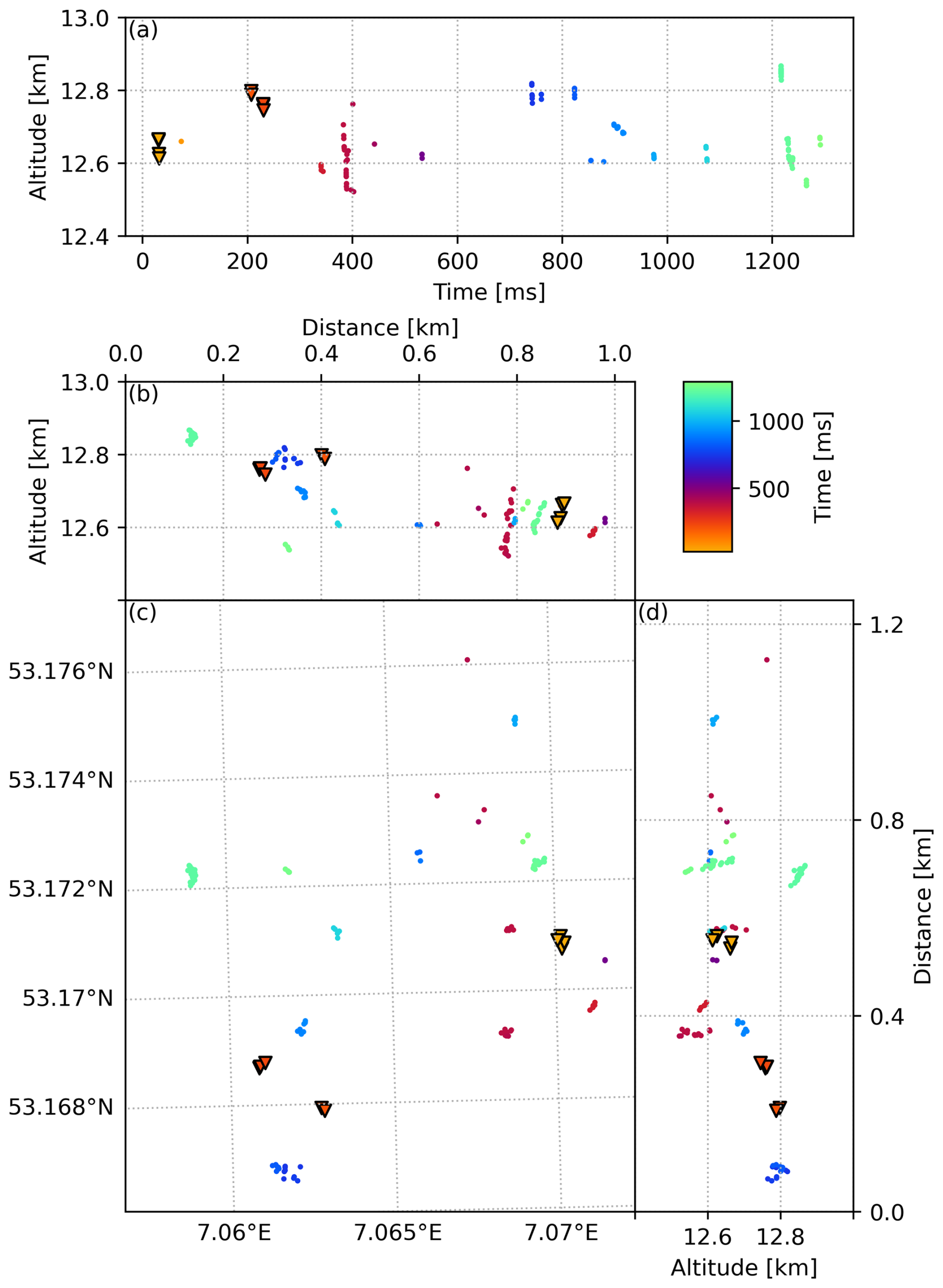
By design, the second stage of clustering in the sparkle classification removes isolated single VHF sources from the sparkle category. We observe three types of isolated VHF sources: (1) isolated VHF sources at low altitudes <5 km that seem to be part of larger, sparsely imaged lightning structures; (2) isolated VHF sources part of dart leaders; and (3) isolated VHF sources in or near the confetti cloud of sparkles. The latter category may be poorly imaged sparkles and can therefore be misclassified as other VHF source. However, given the 2 km radius to select sparkle data, we expect that these misclassifications will only have a marginal effect on the results. The VHF sources at low altitudes and in dart leaders (observations (1) and (2)) are rightfully classified as other VHF sources.

3.2 Storm and Lightning Overview

On 18 June 2021, the atmosphere was very unstable. According to ERA5 data (Hersbach et al., 2023), around 18:00 UTC (all times from here on in UTC) there were places in the Netherlands where CAPE (convective available potential energy) values exceeded 3000 J kg⁻¹. At times, the shear and helicity values exceed 20 and 200 m² s⁻² respectively, for example in Fig. 3. These values are favorable for the formation of supercells. Supercells are a type of convective system characterized by a single very strong updraft, mesoscale rotation in the updraft, and overshooting cloud tops (Markowski and Richardson, 2011). Much turbulence is expected around and aloft the updraft, particularly in the overshooting cloud tops. Supercells typically produce much precipitation, large hail and much lightning (Markowski and Richardson, 2011; Calhoun et al., 2013).

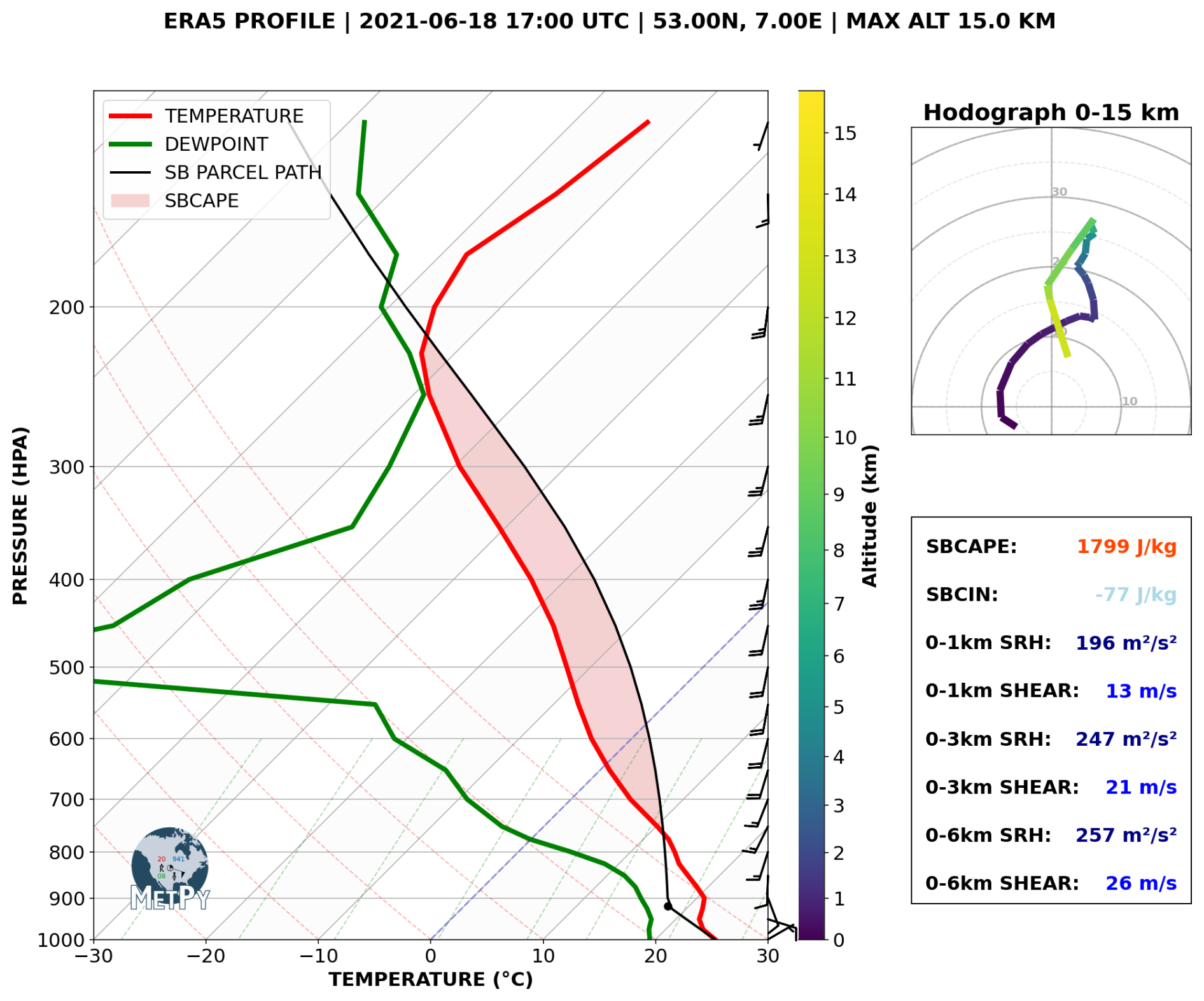
Figure 3 Atmospheric profile and corresponding variables at 17:00, 53° N, 7° E, according to ERA5 data (Hersbach et al., 2023). (a) Skewed-temperature (skew-T) diagram with the absolute air temperature (red), dew point temperature (green), and an air parcel lifted pseudo-adiabatically from the surface (black). Red shading represents the CAPE for pseudo-adiabatic ascent from the surface (SB). On the right axis, wind barbs at different altitudes. In addition to pressure, altitude is indicated next to the color bar. (b) Hodograph with the color scale matching the altitude scale next to panel (a). (c) Helicity (SRH) and wind shear (SHEAR) for different vertical layers.

In the domain of the LOFAR images, there are places until at least 20:00 where CAPE exceeds 2000 J kg⁻¹. The CAPE, shear and helicity values decrease significantly after 20:00, after which conditions become less favorable for any convection to organize into mesoscale structures.

In order to match the LOFAR data with the storm dynamics, we distinguish five different convective systems in the northeast of the Netherlands between 17:00 and 21:00. The different systems are labeled as “A” through “E” in Fig. 4. The convective systems are primarily inferred from radar reflectivity (Z_h) values. The approximate location of lightning as imaged by LOFAR is indicated by black (sparkles) and dark blue (other VHF sources) contours. The locations of sparkles follow from the sparkle classification algorithm as described in Appendix B. In the following, we give give a brief description of the convective systems.

Figure 4 Radar reflectivity scans (1.5° elevation angle) of the storm at the time of the nine different LOFAR images. The black and dark blue contours mark the radar data within a 2 km horizontal distance of sparkles and other VHF sources, respectively. The annotations A–E indicate different convective systems as referred to in Sect. 3.2. The locations of the radar and the LOFAR core are indicated by a pink star and triangle respectively. The (partial) rings centered around the radar indicate the altitude of the radar beam at 2, 4 and 6 km.

Convective system A: Supercell

The reflectivity images in Fig. 4 show that system A persists as an isolated cell with heavy precipitation from ∼ 17:30 to ∼ 19:30. The v-shape, for example in panel d and f, is reminiscent of a supercell. On close inspection, a Bounded Weak Echo Region (BWER) (Lakshmanan and Witt, 1996; Markowski and Richardson, 2011) is apparent. A BWER is a local zone of low reflectivity enclosed by higher reflectivity and is associated with the the strong updraft in a supercell (Musil et al., 1986). The BWER is annotated in Fig. 5, presenting both the top view and a vertical cross section.

Figure 5 Radar reflectivity (Z_h) at 19:17:36 with sparkles superimposed. Panel (a) shows a top view of the 5.5° elevation scan with sparkles projected onto the horizontal plane. Panel (b) shows a vertical cross section along the A–B line in panel (a), with sparkles within 10 km projected onto this plane. 0° and −40° isotherms are indicated by the dashed and dotted white lines respectively. Radar beams from multiple elevation angles are indicated by gray lines, and the 5.5° beam from panel (a) is highlighted in black. The vertical extent of radar data in panel (b) does not reflect the actual 1° beam width. The Bounded Weak Echo Region (BWER) is annotated.

Around 17:20 (not shown), system A splits into two distinct cells, A and A'. The two cells stay close together and are clearly distinguishable in Fig. 4a and 4b. At 17:46:58 (Fig. 4a) and 18:06:44 (Fig. 4b), both cells exhibit lightning, including sparkles. After 18:20, the intensity of A' decays (Fig. 4c–e) and it does not show any lightning in the LOFAR images. This decay happens after another split of cell A around 18:05 (barely visible in Fig. 4).

Convective system B and C

Convective system B first appears relatively disorganized on the Borkum radar reflectivity images. Around 18:20 (not shown), the system organizes itself into a larger, elongated structure. LOFAR images lightning for this system in every image from 18:26:40 onward. Sparkles are found at 18:39:23, 18:58:48, 19:37:29, 19:54:24, and 20:11:51. The image of 20:11:51 only contains a few sparkles.

System C enters the range of the Borkum radar around 18:40. Before that time, it has been active as an isolated convective cell. After 18:40, the convective system starts to grow, and organizes into an arrow shape while catching up with system B. There seems to be interaction between system B and C, and around 19:15 the two systems connect in the radar images. The reflectivity images show a narrow arm extending to the southeast from system C. At 18:39:23, 18:58:48, 19:54:24, and 20:11:51, LOFAR images show lightning in convective system C.

At 19:54:24 and possibly at 19:37:29, LOFAR images show sparkles where the anvil cloud of system C could interact with the anvil cloud of system B. In Fig. 4, the location of the heavy precipitation (high Z_h) does not match well with these sparkles. At higher altitudes, the sparkles do match the location of the highly reflective cloud much better. Therefore, we suspect that for this location, the signal in Fig. 11, is attenuated by the large amount of precipitation in the line of the radar beam. The white ellipse in Fig. 4 marks the area where we expect relatively much effect of attenuation.

Reflectivity images suggest there were mesoscale vortices in both system B and C. These are indicated by the white arrows in Fig. 6. This could indicate the development of supercellular characteristics of the multicellular systems (Markowski and Richardson, 2011).

Figure 6 Top view of Z_h of convective system B (upper part) and C (lower part), at 19:54:24. Two large scale vortices are indicated by the arrows and a region expected to be subject to much attenuation is indicated by the white contour.

Convective system D

Before 15:00, convective system D emerges at the Dutch west coast. Radar reflectivity values show that the system evolves between a state of multiple separated cells, and a north–south oriented line. The latter is for example observed in Fig. 4a. LOFAR images show lightning for system D at 17:46:58, 18:06:44 and 18:26:40. There are only a few VHF sources that are selected by the sparkle classification algorithm.

Convective system E

Around 16:00, south of system D, a convective system emerges that is annotated as E in Fig. 4. Between 17:20 and 18:00, system D, E, and a bow-shaped system seem to interact and form one larger system. This bow-shaped system (not visible in Fig. 4 resulted from a split of system A around 16:30.

From about 18:00 to 18:40, isolated convective cells emerge seemingly spontaneously between the system A, B and C. Since these cell later interact and merge, we also count these individual cells to system E. Eventually, system E moves over the Wadden Sea and it seems to organize into a large single system. LOFAR images show lightning for convective system E at 18:06, 18:26, 18:39, 18:58, and 19:37. The observed lightning is not considered to be sparkle activity.

3.2.1 Mesoscale interpretation

The naming of convective system A–E is inherently subjective, but it does provide a useful framework to distinguish between the lightning characteristics of seemingly separate convective events. We recognize that B, C and the individual convective cells grouped into system E (Fig. 4b–e) were initiated at approximately the same time along a line (approximately North–South oriented). This suggests that this convection was triggered by near-surface convergence forcing upward motion. Cell A appears to have initiated ahead of that line of convergence, but gets gradually overtaken. From 17:20 to about 18:10, system D aligns with this hypothetical line of convergence.

3.3 Quantitative analysis

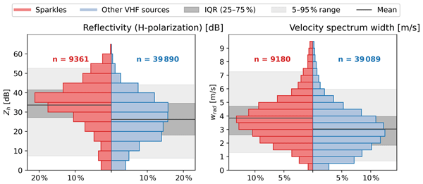
Figure 7 shows histograms comparing the Z_h and W_rad radar data near sparkles to radar data near other VHF sources. The Z_h and W_rad values are very different near sparkles. The average Z_h and W_rad values are higher (see Table 2 and black lines in Fig. 7) for sparkles. The distribution of sparkles also show a heavier tail for higher values. KS p-values are well below 1 %, indicating a statistically significant difference between sparkles and other VHF sources. Sensitivity tests (see Sect. S2 in the Supplement) show that these results are not sensitive to varying the radius to collect radar data near VHF sources, or varying the parameters for sparkle classification. Comparing the radar data at different altitudes (see Sect. S2 in the Supplement), the Z_h values are significantly higher at all altitudes. For W_rad, the values are only significantly higher below 12 km altitude.

Table 2 The mean values, Kolmogorov–Smirnov statistics, corresponding p-values, and Cliff's δ, for the distributions of Fig. 7.

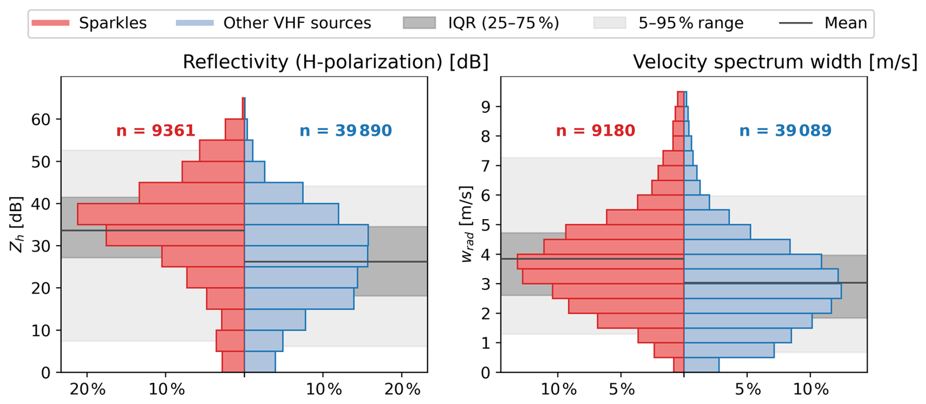
Figure 7 Histograms of radar reflectivity Z_h and radial velocity spectrum width W_rad near sparkles compared to radar data near other VHF sources, according to the selection procedure described in Sect. 2.3. The number of radar data points are indicated by the number n. The solid black line, dark and light shading represent the mean, interquartile range, and 90 % quantile range respectively.

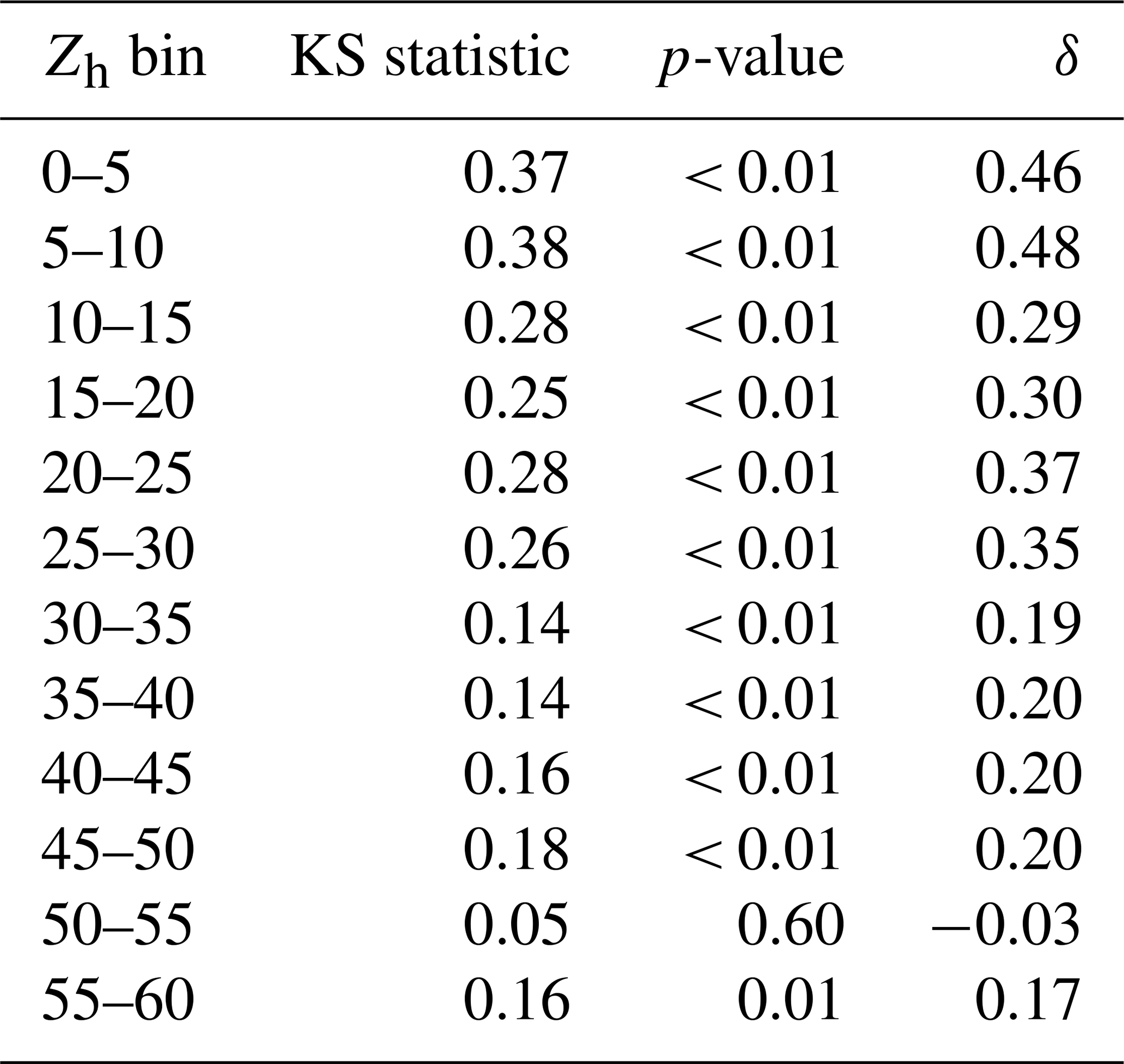
Figure 8 shows histograms of Z_h versus W_rad, allowing to investigate their correlation. In the panel b and d, where the number of counts are normalized per Z_h bin (vertical columns), we observe a nonlinear correlation. Panel f, the difference between panel b and d, shows that the W_rad values are consistently higher for values of Z_h<50 dBz. The KS statistic and Cliff's δ per Z_h bin are provided in Appendix C.

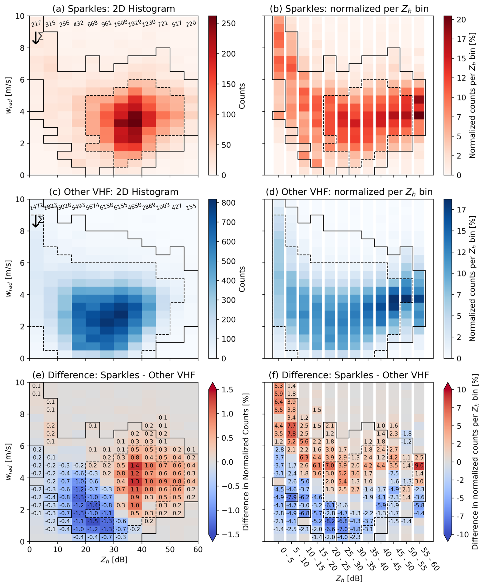
Figure 8 Two-dimensional histograms of the radar data near sparkles. To indicate the significant data range, solid and dashed contours show where the number of data points in a bin exceeds 10 and 50 respectively (a, b), the radar near other VHF sources (c, d), and the differences thereof (e, f). The histograms in panel (b) and (d) are normalized per Z_h-column. Panel (a) and (c) are counts per Z_h-W_rad-bin. The number of counts per Z_h-column are annotated on top. In panel (b) and (d), the histograms are normalized with the number of counts in each Z_h-column. Panel (e) shows the difference between the normalized versions of (a) and (c). Panel (f) shows the difference between panel (c) and (d). The annotations of (e) and (f) correspond to the values and corresponding shading.

Figure 9 shows the results of the HMC algorithm. For sparkles (red), a relatively larger percentage of radar data is classified as graupel/hail (GH). Near other VHF sources (blue), more data classified as ice crystals or dry snow. Figure 9b and c can be used to estimate the quality of the HMC algorithm. The performance of the HMC algorithm for each category can be estimated both with the maximum mean probability for each row, always found on the diagonal, and with the difference between the probabilities on each row. A larger difference between the maximum and other probabilities, indicates a better classification. The results show that the the “Graupel/Hail” and “Hail” classification are relatively certain, with a difference of ∼ 0.3 between the maximum and second highest mean probability. In contrast, the HMC algorithm has much more difficulty in distinguishing between “Dry Snow”, “Horizontal Ice Crystals”, “Vertical Ice Crystals” and “Light Rain” categories. These categories have a difference of ∼ 0.1 between the maximum and second highest mean probability. Regarding the orientation of ice crystals, we see relatively more vertical aligned ice crystals (VC) for sparkles. The opposite holds for other VHF sources.

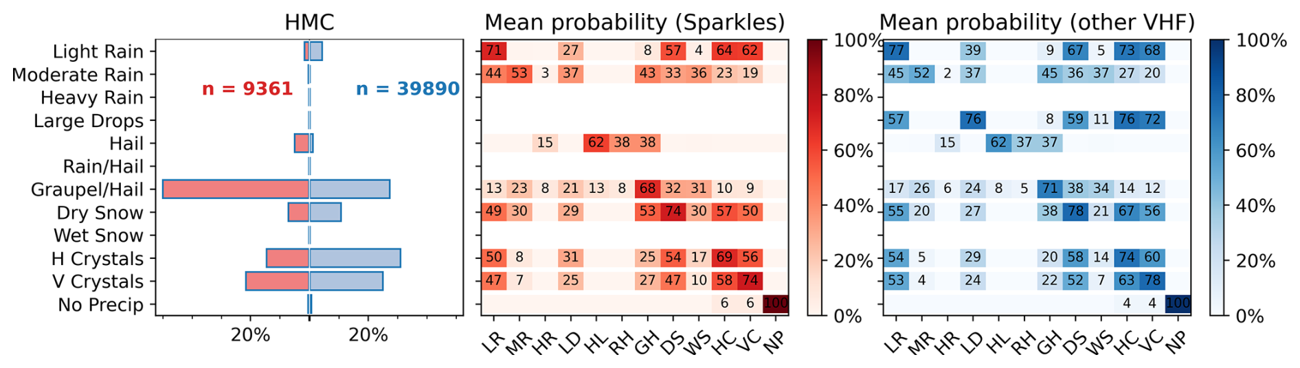
Figure 9 Panel (a) shows a histogram of the hydrometeor classification (HMC) algorithm for radar data near sparkles (red) and other VHF sources (blue). The number of included radar data points is indicated by the number n. Panel (b) and (c) show the probabilities for different hydrometeor types from the HMC algorithm, averaged over the data points in each bar of panel (a).

3.4 Qualitative analysis

In order to understand the quantitative results in Sect. 3.3, we have also inspected the individual radar images. Figures 10, 11 and 12 show radar images with an overlay of contours to mark data corresponding to “sparkles” and “other VHF” sources. Note the threshold of 8 km altitude and the 0 dB reflectivity that is used to select radar data. Figures for additional radar elevation angles, for system A and B at times corresponding to LOFAR observations can be found in Sect. S4 in the Supplement.

Figure 10 Top view of radar images at an elevation angle of 17°, around convective system A, at the time of the LOFAR image at 19:17:37 UTC with: (a) reflectivity Z_h, (b) radial velocity V_rad, (c) radial velocity spectrum width W_rad, (d) the Hydrometeor Classification Algorithm HMC. The radar resolution volumes within 2 km of sparkles (black dotted) and other VHF sources (blue dashed) are indicated by contours. Arrows indicate cloud edges with high W_rad values. Yellow arcs indicate the 8 and 12 km altitude of the radar data.

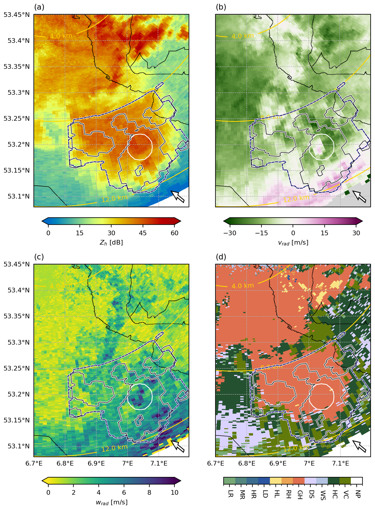
Figure 11 Similar to Fig. 10, but corresponding to the LOFAR image at 19:54:24, and at an elevation angle of 12°, focusing on system B. The white circle indicates an updraft column. Arrows indicate cloud edges with high W_rad values. Yellow arcs indicate the 4, 8 and 12 km altitude of the radar data.

Figure 12 Similar to Fig. 11, but at an elevation angle of 17°. The white circle corresponds to the location of the white circle in Fig. 11. Arrows indicate cloud edges with high W_rad values. Yellow arcs indicate the 8, 12, and 16 km altitude of the radar data.

A first observation is that the radar data near sparkles is always a subset of the radar data near other VHF sources. Although it is possible that large lightning structures exist in the same volume as sparkles, it is also possible that this is an effect of an incomplete sparkle classification algorithm. As mentioned in Sect. 2.3, incomplete sparkle clustering should have marginal effects on the statistics presented in section 3.3, because the subset of radar data near “sparkles” is excluded from the radar data near “other VHF” sources.

In general, the radar images often show high W_rad values where the radar beam exits a precipitation cloud at high altitudes. These areas often have low Z_h values and they likely mark the interface between the stratosphere and precipitation cloud. The cloud-stratosphere interface with low Z_h and high W_rad values are seen in the leftmost columns of Fig. 8e and f.

As expected from the histograms in Fig. 7, we see that the sparkles are often found in areas with high reflectivity values. We also note that within the sparkles data (black dotted contour), the radial velocity V_rad shows much divergence and rotation. This is seen in the images as the radial and cross-radial gradients in the V_rad values respectively. The images show that locations with rotation and divergence are often accompanied by local points of relatively high W_rad values.

In Figs. 11 and 12 we observe that sparkles mainly surround the location of an intense, isolated updraft column. The approximate location of the updraft column at ∼ 10 km is indicated by a white ellipse. This ellipse marks a patch of positive V_rad values (∼ 1 km²) surrounded by negative V_rad values. Such a V_rad pattern could be caused by (1) high vertical velocities in the updraft that overcome hydrometeor sedimentation, (2) mesoscale rotation of an updraft, or a combination of (1) and (2). The intensity of the updraft is highlighted by the observation that the Z_h values are > 40 dB at the location of the positive V_rad patch. Only a strong updraft would offset the large sedimentation velocities that are associated with Z_h>40 dB values. We also note the relatively high W_rad values around the updraft column.

The location of the Z_h core in Fig. 12 is displaced ∼ 0.05° from the location of the updraft at ∼ 10 km (white ellipse). However, this displacement is roughly the same throughout the whole convective system. Therefore the displacement is probably related to advection between the different radar scans and the slanted orientation of the updraft columns. In Fig. 12, aliasing of the V_rad signal gives ambiguous rotation and divergence in the updraft column. However, we do clearly see local points of enhanced W_rad values for the patch of sparkle data.

For Fig. 10, one can use similar observations of positive V_rad patches where Z_h values are high to find two or three updraft columns. However, these locations are not so isolated as the updraft seen in Fig. 11. The locations are not indicated.

In accordance with the statistics in Fig. 9, the radar images show that locations of sparkles are correlated in regions that have been classified as graupel or hail (GH). Especially at high altitudes, for example in Fig. 12, we see that the sparkles data is more limited to areas that have been classified to feature graupel or hail (GH), whereas the other VHF data encompasses vast areas that have been classified to feature ice clouds (HC and VC).

4 Discussion

4.1 Sparkle classification

Given the clustering parameters as presented in Sect. 2.2, the sparkle classification algorithm yields satisfactory results. Given the proximity in space, we acknowledge that some small clusters (e.g. Fig. 2) and some isolated VHF sources may be misclassified as other VHF sources. We expect that the impact of such false negatives is marginal. Considering the 2 km radius to select radar data, many of the false negatives would be masked by the proximity of sparkles. We also note that changing the algorithm to reduce false negatives, for example by increasing the minimum number of VHF sources for a large cluster or by omitting the second stage of small-scale clustering, leads to more false positives. This is unfavorable for the selection of radar data, because the 2 km radius near sparkles gets priority over the 2 km radius near other VHF sources.

Scholten et al. (2023) show that some small‐scale discharges are similar to so called “needles” discharges, and are related to positive‐leader breakdown. Our two‐stage clustering (first stage temporal margin t=0.3 s) is likely to merge such rapid, localized needle pulses, and any accompanying dart leaders, into larger clusters. Consequently, our results only represent sparkles that are not clearly linked to positive‐leader breakdown.

4.2 HMC algorithm

Although the classification for graupel/hail (GH) is relatively certain, panel b and c in Fig. 9 show that the distinction between horizontal crystals, vertical crystals, dry snow, and light rain is more uncertain. Therefore, we can not draw substantiated conclusions about any electric field effects on ice crystal alignment. On the other hand, we are confident that the surroundings of other VHF sources are often filled with ice crystals. For sparkles, the surroundings are dominantly filled with graupel/hail, but almost equally much space with ice crystals. That is, if we aggregate the horizontal and vertical ice crystals into one hydrometeor category.

Another aspect to consider for the fuzzy-logic algorithm is that it was originally designed for S-band radars. Because of their larger wavelength, S-band radars are less prone to Mie scattering and attenuation (Straka et al., 2000). Although previous work (Marzano et al., 2006; Overeem et al., 2020; Vulpiani et al., 2012a) has shown the potential of fuzzy-logic algorithms for C-band radars, attenuation and Mie scattering remain a source of error. The algorithm we use in this paper does compensate for Mie scattering, but no attempt is made to compensate for attenuation. For improved results, one may attempt a more complicated scheme to weight the different polarimetric variables, following Dolan et al. (2013).

4.3 Physical interpretation

Placing our results in the context of previous work, the following similarities are found. The correlation between high reflectivity values and sparkle-like lightning is also found by Emersic et al. (2011), Calhoun et al. (2013) and MacGorman et al. (2017). These studies also observe that these discharges form a cap on top of a very strong, vertical updraft, reaching high altitudes. Our study also suggests that sparkles are found at the top or above strong updrafts, based on three arguments. Firstly, the high reflectivity values at sparkle altitudes can logically only be present in or near updrafts. The large hydrometeors responsible for such high reflectivity values would quickly sediment down to lower altitudes were it not for the presence of strong updrafts. Secondly, the V_rad radar images indicate updrafts. For both system A and B, the images (see Sect. S4 in the Supplement) at low elevation angles show mesoscale rotation, indicated by cross-radial V_rad gradients, at locations with high Z_h values. For the radar image in Fig. 11, we even see a patch of positive V_rad values at about 10 km altitude, well above the low-level rotation. This indicates that the updraft extends up to more than 10 km altitude. Figure 12 shows the location of sparkles, just above this location. Thirdly, the relative location of the BWER and hook echo in system A indicate that the main updraft is much aligned with sparkles, especially when one considers that the updraft is likely to be slanted by wind shear. Unfortunately, time differences up to 2.5 min between radar and LOFAR data, broadening of the beam width, and the few radar elevation angles reaching sparkle altitudes (see Appendix A) inhibits the quantification of the distance between sparkles, updrafts, and cloud tops.

All of the aforementioned studies also specifically associate the sparkle-like discharges with the intensification of updrafts. The ∼ 20 min gap between LOFAR images complicates a detailed temporal analysis of sparkles. However, if the convective systems that produce sparkles are indeed a supercell and a squall line, it may be expected that updrafts were intense. The story line of the mesoscale events in convective system A, such as the development of a BWER and hook echo, would suggest intensifying updrafts around the time of sparkles. For convective system B, there are few mesoscale features that indicate the updraft intensification matching the presence of sparkles. However, we think that attenuation obscured some of the dynamical features of the right-hand-side of system B (see Fig. 6), which produced many sparkles.

We are confident that for high Z_h values, the higher W_rad values near sparkles are mainly reflecting the enhanced atmospheric turbulence near sparkles. Turbulence enhances W_rad through wind-shear within the radar resolution volume (sub-resolution). Not only does wind shear drive turbulence, but the chaotic fluctuations of wind shear also constitute turbulence. Qualitative comparison shows that, for higher reflectivity values, enhanced W_rad values are generally accompanied by wind shear between radar resolution volumes. Thus, the driver for sub-resolution turbulence in cloud tops is clearly visible. Examples can be seen in Figs. 10 and 11 as spatial gradients in the V_rad image, at locations where both Z_h and W_rad values are high.

For low reflectivity values, it is likely that side-lobe contamination plays a role in enhanced W_rad values. This effect is most pronounced if, the Z_h value for a specific radar resolution volume is not high, bu Z_h values are high in the surroundings. In this case, the radar beam's side-lobes, which also probe the volume outside the targeted resolution volume, contribute disproportionally to the total returned signal. Because a larger volume contributes to the total signal, measured wind shear, and thus W_rad values, can increase. Examples of locations that are likely to be the result of side-lobe contamination, are marked with the arrows in Figs. 10–12.

Side lobe contamination explains the high W_rad values observed in Fig. 8 for the lowest Z_h bins. From Fig. 8f, it appears that the side-lobe contamination is more prominent for sparkles. This can be expected because the sparkles are, more often than other VHF sources, concentrated near highly reflective updraft columns. It is near these updraft columns that the spatial Z_h gradients, and thus side-lobe contamination is largest. Since side-lobe contamination is most significant for low Z_h values, we are confident that the observed W_rad enhancement actually represents atmospheric turbulence for Z_h>15 dB.

Another mechanism that can increase W_rad values, is differential sedimentation of mixed hydrometeors. However, because the radar elevation angles are relatively low (≤25°), the sedimentation velocities, which are inherently vertical, are a minor contribution to the spectrum of the velocity in the direction of the radar beam. Additionally, this type of enhancement is most pronounced when the backscattered signal is not dominated by a single type of hydrometeor. The HMC algorithm shows, comparing the numbers between the rows in Fig. 9, that the uncertainty in the classification is similar for both sparkles and other VHF sources. Therefore, we conclude that for sparkles, there is no increased hydrometeor mixing and thus no enhanced W_rad through differential sedimentation.

The presence of intense turbulence near sparkles, as suggested by the enhanced W_rad values, may be important for the relevant charging mechanisms that explain the presence of these small-scale lightning structures.

Non-inductive charge separation is generally considered to dominate the charging mechanism in thunderclouds. However, the inductive charging might be considerable in certain conditions. Mareev and Dementyeva (2017) showed that for turbulent conditions, an ambient electric field and hydrometeors of adequate size, the inductive charging mechanism may lead to exponential growth of the electric field. Supposing that the local spots of enhanced W_rad values represent the fine scale turbulence needed for significantly enhance the inductive charging mechanism, this could explain the intermittent behavior of sparkles that is observed by LOFAR.

In light of the small spatial extent of sparkles, we evaluate mechanisms that could form charge pockets and thereby limit growth of sparkles. Modeling work by Calhoun et al. (2014) shows that charge pockets may be related to heterogeneous charging in the updraft column. Turbulence in cloud tops could fragment those pockets down to the ∼100 m length scale associated with sparkles. Our results do not clarify the role of heterogeneous updraft charging. However, given our observation of increased turbulence near sparkles, turbulent fragmentation seems plausible. The size of the charge pockets in the study from Brothers et al. (2018) do match well with the size of sparkles. They show that small charge pockets are abundantly generated at the top of the updraft of a supercell. The main mechanism for the small extent of charge pockets are turbulence with length scales > 250 m (resolved in their simulations). However, the unresolved (< 250 m) turbulence can also play a significant role for further fragmentation of charge pockets. The increased turbulence that we observe in the vicinity of sparkles and their location to the updraft columns, matches well with the results from Brothers et al. (2018). Alternatively, some works suggest that velocity gradients at the top of overshooting clouds may cause folding of a charged screening layer into the cloud (MacGorman et al., 2017; Emersic et al., 2011; Calhoun et al., 2013). The folding process could potentially form pockets of the oppositely charged screening layer wrapped into the cloud. If so, we would expect to see a complex V_rad pattern along the top-edge of the cloud. In Fig. 11b, near sparkles (black dotted contour), we indeed see a “frayed” pattern in the V_rad gradient at between 11 and 12 km altitude. Folding in cloud tops could also be related to the irregular coiled shapes in both the Z_h and V_rad images near sparkles. We also note that the mechanism to drive screening layer folding, namely wind shear, may be visible as enhanced W_rad values at the top-edge of clouds. For example near the 12 km contour line of Fig. 10. However, we cannot distinguish tropopause wind-shear from side-lobe contamination (arrows in Figs. 10–12).

Altogether, our observations are compatible with both hypotheses of (1) folding of a screening layer into the cloud, and (2) turbulent mixing of larger charge regions into small charge pockets. These mechanisms may act jointly.

As suggested by Calhoun et al. (2013), the proximity of the charged screening layer to the lofted charge in the updraft might enhance the electric field. If proximity to the screening layer is indeed a condition for sparkle discharges, it could explain why turbulence in and near the updraft has enough time to form small change pockets. Our results results near sparkles, with reflectivity values and graupel/hail classification indeed suggest that the lofted charge, carried by large hydrometeors, is brought relatively high and thus close to a screening layer. However, with our coarse vertical radar resolution, we are unable to check the distance of sparkles to a charged screening layer.

4.4 Outlook

This study uses a unique combination of high resolution lightning data and operational weather data. Further research with similar methods may disclose the location of sparkles with respect to a charged screening layer, charge pockets, and enhanced turbulence.

A first improvement for future studies will come with the release of LOFAR 2.0, planned for 2027. The new system can observe significantly more flashes per storm. This will allow a better comparison of the temporal development of lightning and sparkles with the thunderstorm dynamics.

It would be most useful to deploy a mobile research radar for the study of sparkles. Using more steep elevation angles, potentially with an adaptive scanning strategy that focuses on the overshooting cloud tops, would allow to get a much higher vertical resolution in the location which is most relevant for sparkles. Additionally, an extended analysis of the radar data, for example, a spectral analysis similar to Mak and Unal (2025), could provide more information on the mixture of different hydrometeors and the source of the observed W_rad enhancement.

Finally, the instruments aboard the Meteosat Third Generation (MTG) satellite (Holmlund et al., 2021) that was launched in 2022 could provide useful information on the relation between cloud top height and lightning. In particular, matching the MTG lightning data with LOFAR lightning images may reveal whether the sparkles occur above the clouds.

5 Conclusions

In this study we have investigated the atmospheric conditions associated with the occurrence of small-scale intermittent lightning discharges at the top of thunderstorms, called “sparkles”. To this extent, we have compared volumetric weather radar data with LOFAR high-resolution lightning images. Our results show that sparkles occur near high radar reflectivity values at high altitudes. Such values are associated with strong updrafts, lofting of graupel, and overshooting cloud tops. An algorithm for hydrometeor classification confirmed the dominance of graupel near sparkles. In the proximity of sparkles, we also observe enhanced W_rad values and heterogeneous V_rad patterns. We are confident that this signal represents enhanced turbulence near sparkles. We hypothesize that the turbulence, through the creation of charge pockets, is crucial for the small spatial extent and intermittent behavior of sparkles. It is not evident if turbulence plays a role solely by mixing, or also through enhanced inductive charging.

Both convective systems with sparkles had supercellular characteristics. Additional LOFAR observations of sparkles are needed to find out if sparkles could also live in weaker or less organized convective systems.

Our findings may have a practical application for now-casting of severe weather. We show that the presence of sparkles reveals severe thunderstorms and the location of intense updrafts. Therefore, implementation of a sparkle detection algorithm on live high resolution lightning data, would provide a fast way to warn for meteorological hazards that accompany severe thunderstorms.

Although our results do not fully clarify the hypotheses about the physics of sparkles, our research does pave the way for further research. Our methods may serve as inspiration for future research comparing LOFAR lightning images with radar data. Furthermore, our conclusions could be used as a starting point for research with a more bottom-up approach to study atmospheric perquisites for, and the physical mechanisms of, sparkles. Such future research could consider our proposed hypotheses of turbulent enhancement of inductive charging.

Appendix A: Radar data

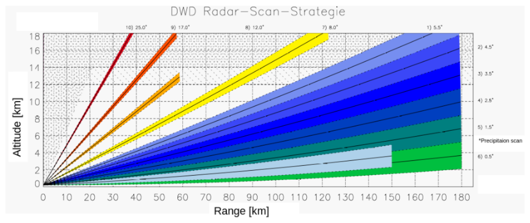
Figure A1 Adapted version of figure from Frech et al. (2017). Scanning strategy of the DWD radar on Borkum. Different radar beams and the 1° beam width are represented by shadings. The corresponding elevation angles are shown at the side of the axes. Note: the precipitation scan is not used in this study.

A1 Borkum radar

The Borkum radar has a frequency range of 5600–5650 MHz (C-band). It scans the atmosphere at 10 elevation angles between 0.5° and 25° with a beam width of 1°, and a range bin separation of 250 m. Figure A1 shows a diagram of the scanning strategy with the elevation angles. The volume scanning procedure is repeated every 5 min. The raw data was processed by the German Meteorologival service (Deutsches Wetterdienst). For detailed information about the radar and data, we refer the reader to Frech et al. (2017).

A2 Radar errors

The frequency of the polarimetric radar determines the sensitivity to different types of hydrometeors. C-band radars are most suitable for particles with a diameter between approximately 0.5–7 mm. Smaller particles hardly scatter the radar pulse and large particles may cause resonance effects. Resonance effect may cause very high Z_h values and spatial discontinuities in the scatter properties. This means that large hail stones, snow flakes or very large droplets may complicate the interpretation. In this study, corrections are made for resonance effects for the computation of the specific phase difference ϕ_dp. The ϕ_dp variable is used in the computation for HMC. The algorithm is described in Appendix B.

For C-band radars, attenuation of the radar can be considerable. The blockage of the radar beam by a highly reflective atmosphere will decrease the measuring skill behind. This may introduce a negative bias of Z_h. For V_rad and W_rad, attenuation increases the uncertainty. In this study, we do not correct for attenuation.

Appendix B: Data processing

ERA5 data

We use the ERA5 reanalysis data (Hersbach et al., 2023) for the ambient temperature (in the HMC algorithm) and the horizontal wind velocity (advection of radar data). The ERA5 data is hourly and comes on fixed pressure levels. We used the geopotential to convert the ERA5 data to the height, and interpolate linearly in space and time to the radar data points.

B1 Geospatial data processing

There are two important factors to consider for a valid spatial analysis, the georeferencing of the radar data and the time difference between radar and LOFAR data.

For georeferencing the radar data, the wradlib.georef.georeference algorithm (Heistermann et al., 2013) has been applied. This algorithm makes uses of the equations provided (Doviak et al., 1993) that take into account the curvature of the earth and the refractive index of the atmosphere. A standard value of $k_e=\mathrm{4}/\mathrm{3}$ is used as the refractive index compensation factor.

The native output of this wradlib Python algorithm is in an azimuthal equidistant projection. For comparison, LOFAR data is converted to the same azimuthal equidistant projection. All figures that include radar data have the radar's native azimuthal equidistant projection.

In order to deal with the time difference Δt between LOFAR data and radar data, we apply advection to the radar data to match the time of LOFAR images. In this study, we perform no temporal interpolation of the radar data. Instead, we use the time of the LOFAR image of interest and we collect the radar scans at each elevation angle that are closest in time. Subsequently, we linearly interpolate the the horizontal wind velocities of the ERA5 data of 18 June 2021 in time and space on to the location of each radar data point. This yields the horizontal wind vector v_i, corresponding to each data point with index i. These values are used to move the georeference x_i of the each radar data point over a distance of $\mathrm{\Delta }{\mathit{x}}_i=\mathrm{\Delta }{t}_i\cdot {\mathit{v}}_i$. Here, Δt_i is the time difference between the LOFAR data and each radar data point.

In practice, the advection scheme moves the radar data up to 3 km. This is not surprising given the maximum time difference of 150 s for the 5 min radar scanning procedure and the high altitude wind velocities of more than 30 m s⁻¹. Within one sweep there are sometimes be significant differences in advection shifts. Especially between the first and last scanning azimuth. Although the data is adjacent in space, a time difference of ∼20 s gives a large jump in advection distance. Another large jump in advection distances is visible where the radar beam intercepts the tropopause. This is a result of significant wind gradients at this altitude.

To reduce computational cost, the ERA5 altitudes are replaced by the average altitude of each model level. As a results, the ERA5 data is structured on a Cartesian grid and the interpolation towards the radar data points is less costly.

Convective systems can move with a different velocity than the ambient wind, and thus there may be errors in the distance of horizontal advection. As an alternative, we also tried advecting with the propagation velocity of the convective cells. This velocity field was determined using the 2-dimensional radar composite at 1500 m altitude and pySTEPS' Lucas-Kanade algorithm. Differences in advection distances are shown in Fig. B1. Between the two methods, we see differences up to 2 km and an average difference of 330 m advection. However, the quantitative results are not noticeably different. Differences are likely mitigated by the 2 km radius which is used to select radar data near VHF sources.

For our analysis, we choose to use the ERA5 velocity data, because it is independent of the choice of tracking algorithm. Furthermore, the cell motion at 1.5 km altitude, may be shifted and potentially different from the radar data above 8 km that we consider in our analysis.

B2 Matching radar and LOFAR data

The scipy.spatial.KDTree.querry_ball_point function is used for collecting the radar points within a radial distance of the LOFAR data. In all results, a radial distance of 2 km is used as a threshold for proximity. This is a subjective choice, that seems reasonable keeping in mind the poor vertical radar resolution up to 4 km, the temporal radar resolution of 5 minj, and the uncertainties in advection over such timescales.

B3 Computing K_dp

The cumulative differential phase ψ_dp is included in the Borkum radar dataset. We use the wradlib Python package (Heistermann et al., 2013) for filtering and computing the differential phase shift ϕ_dp and the specific differential phase K_dp values. The result is highly depend on filtering and correction choices. The used algorithm and filtering steps are explained in Sect. S1 in the Supplement.

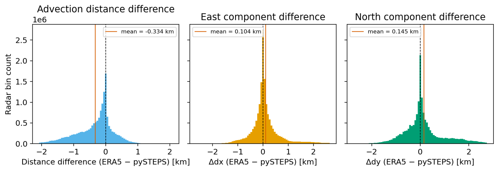
Figure B1 Histograms of differences in advection distance between ERA5 wind-based advection and advection based on pySTEPS’ Lukas–Kanade convective cell motion tracking. (a) Absolute difference in the advection distance. (b) Difference in the longitudinal component. (c) Difference in the latitudinal component.

Appendix C: Statistical results per Z_h bin

Table C1 For all Z_h bins in Fig. 8 (columns on the right panels): two-sample Kolmogorov-Smirnov statistic, corresponding p-value, and Cliff's δ.