Drivers of Atmospheric Volatile Methylated Sulfur Variability Across the Southern Ocean and Antarctic Coast

Biogenic volatile methylated sulfur (VMS) gases, dimethyl sulfide (DMS) and methanethiol (MeSH), are major precursors of climate-cooling sulfate aerosol, yet their sources, co-emission and fate remain poorly constrained over the Southern Ocean and Antarctica. In this study, we combine atmospheric VMS measurements with biogeochemical and meteorological observations from an austral summer Southern Ocean voyage to examine the drivers of atmospheric VMS concentrations across contrasting ocean-atmosphere regimes. At the Antarctic Ice Edge (62–67° S), DMS dominated the VMS burden (up to 5.7 ppb) with episodic coastal polynya and shelf biological hotspots demonstrating very low MeSH : DMS (0.3 %–4 %). In this regime, DMS variability was strongly related to recent air mass exposure to high surface chlorophyll a (R² = 0.49), whereas MeSH showed little dependence (R² < 0.14), consistent with stronger heterotrophic control on MeSH production. Over the open ocean (32–62° S), DMS and MeSH were tightly coupled (R² = 0.80) with higher MeSH (up to 250 ppt) and MeSH : DMS (∼ 15 %), but chlorophyll a explained little of the variability (R² = 0.15); instead, physical ocean structure and boundary-layer conditions influenced VMS variability. DMS and DMSO co-varied at the Antarctic Ice-Edge (R² = 0.69), indicating rapid oxidation via addition reactions with hydroxyl and bromine monoxide radicals at the surface. Overall, our results support developing coupled VMS–biogeochemical parameterisations to better capture aerosol–cloud representation in Southern Ocean climate models, and revising DMS-based parameterisations of MeSH at the Antarctic Ice-Edge, which currently appear to overestimate MeSH contributions to the VMS burden under these conditions.

1 Introduction

The ocean-atmosphere exchange of dimethyl sulfide (DMS) represents the largest natural source of biogenic sulfur to the global atmosphere (Simó, 2001; Bates et al., 2004). Produced via enzymatic cleavage of the algal precursor dimethylsulfoniopropionate (DMSP), DMS accounts for up to 70 % of natural sulfur emissions (Lana et al., 2011; Kettle et al., 1999) and exerts strong influence on sulfate aerosol formation, cloud properties, and climate (Andreae and Crutzen, 1997; Hodshire et al., 2019; Mahajan et al., 2015). The Southern Ocean plays a disproportionately important role in this cycle, contributing nearly 60 % of global DMS emissions (Zhou et al., 2024), yet it remains persistently under-observed and poorly represented in models (Mallet et al., 2023a; Hulswar et al., 2022). Co-emitted volatile methylated sulfur (VMS) species, especially methanethiol (MeSH), may also have important climatic impacts, with the Southern Ocean representing an estimated 27 % to global emissions (Wohl et al., 2024; Tashmim et al., 2025). However, the production pathways and atmospheric budgets for MeSH in this region remain poorly constrained, further limiting our understanding of biogenic VMS contributions to Southern Ocean aerosols.

The Southern Ocean provides a rare natural environment where aerosol–cloud interactions are dominated by marine sources, with limited anthropogenic and terrestrial influence (Hamilton et al., 2014; Schmale et al., 2019). Strong spatial and seasonal gradients in sea-ice retreat, iron supply, and mixed-layer depth, lead to highly variable phytoplankton community abundance and structure and therefore biological production of DMSP (McNabb and Tortell, 2023; Sokolov and Rintoul, 2007; Hayward et al., 2024; Heidemann et al., 2024; Wright et al., 2010). These physical–biogeochemical regimes can shift rapidly near the Antarctic coast, giving rise to short-lived but extreme VMS emissions events (Webb et al., 2019; Levasseur et al., 1994; Koga et al., 2014) that remain difficult to capture in coarse climatologies (Ishino et al., 2026).

Chlorophyll a (Chl a) is often used as a proxy for phytoplankton biomass, and therefore as an indirect predictor for DMS (McNabb and Tortell, 2023; Jarníková and Tortell, 2016; Halsey and Giovannoni, 2023; Manville et al., 2023; Zhang et al., 2020). However, ambiguous relationships between DMS and Chl a have been reported in such studies, suggesting additional controls on DMS production, emission, and loss over seasons and regions (Manville et al., 2023). Global surface ocean DMS climatologies (e.g., Kettle et al., 1999; Lana et al., 2011; Jarníková and Tortell, 2016; Hulswar et al., 2022) show their largest discrepancies across the Southern Ocean, where the highest DMS concentrations, particularly those associated with marginal ice zone blooms, are sparsely observed and often omitted. Emerging climatologies for MeSH (Wohl et al., 2024; Tashmim et al., 2025) indicate it may substantially enhance sulfate aerosol burdens, but there are very few seawater and atmosphere MeSH measurements across the Southern Ocean (Lawson et al., 2020; Wohl et al., 2024; Rocco et al., 2025; Mynard et al., 2025b) and MeSH is yet to be routinely incorporated into models, limiting our understanding of its climatic role.

This poses the challenge of understanding whether the more frequently measured seawater and atmospheric DMS can act as a reliable proxy for MeSH emissions, as presented in Wohl et al. (2024); Tashmim et al. (2025); Jacob et al. (2026). Both VMS gases originate from DMSP, but their relative production is highly dependent on phytoplankton taxonomy and physiological state, heterotrophic cycling, and environmental conditions, all of which vary dramatically across the Antarctic ice-edge and the wider Southern Ocean (Hayward et al., 2024). Mynard et al. (2025b) demonstrated a consistently strong relationship between DMS and MeSH over the open Southern Ocean; however, it changes south of the Polar Front along the Antarctic coastline, as a result of unique air‐mass histories and contrasting continental, ice‐edge, and marine bloom influences that produce distinct MeSH : DMS regimes.

Despite their central role in the sulfur cycle, the fate of VMS species remains incompletely understood. As Fig. 1 illustrates, DMS is primarily oxidised by hydroxyl radicals (OH), producing either sulfur dioxide (SO₂) (and ultimately sulfuric acid) via the H-abstraction pathway, or dimethyl sulfoxide (DMSO) and eventually methanesulfonic acid (MSA) via the OH-addition pathway, with both pathways contributing to sulfate aerosol (Hoffmann et al., 2016; Wang et al., 2021). The branching between these pathways is highly sensitive to temperature and to some extent to halogen chemistry, particularly bromine activation in high-latitude marine boundary layers (Breider et al., 2010; Saiz-Lopez et al., 2007; Read et al., 2008; Jang et al., 2022). MeSH oxidation pathways are incompletely understood, with recent model representation of MeSH emission and oxidation assuming 100 % conversion to SO₂ (Novak et al., 2022; Wohl et al., 2024). However, this may overestimate MeSH contributions to SO₂ at low temperatures. Recent laboratory and modelling studies have provided evidence for non-SO₂ producing MeSH oxidation pathways leading to MSA formation as well as SO₂ and H₂SO₄ (Berndt et al., 2023; Chen et al., 2023; Tashmim et al., 2025); however, the contributions of these pathways to aerosol yields observed in the atmosphere remain uncertain.

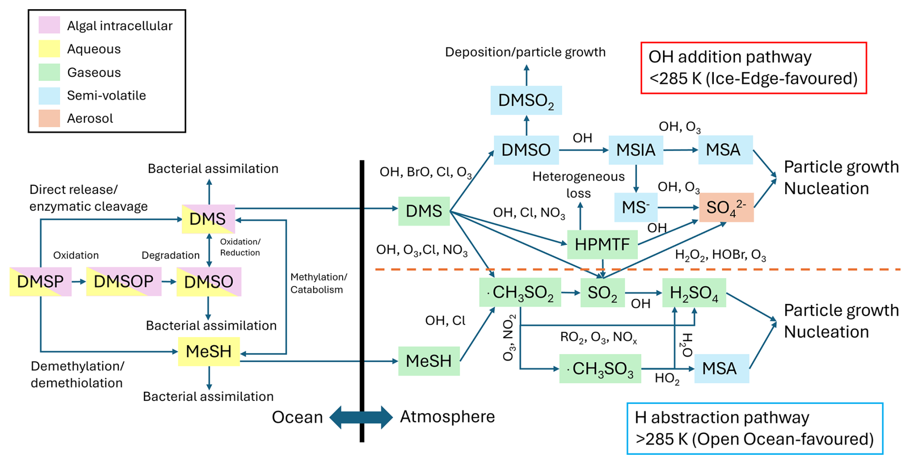
Figure 1 Simplified chemical transformations for climatically relevant pathways of VMS emissons and oxidation. Yellow boxes indicate aqueous phase, pink boxes indicate algal intracellular processing, green boxes indicate gas-phase, blue boxes indicate semi-volatile and red boxes indicate aerosol-phase.

Together, these key uncertainties in the polar biogenic sulfur cycle, and the fact that their underlying processes remain under-represented in current numerical models, underscore the need for high-resolution, co-located measurements of DMS, MeSH, their oxidation intermediates, and the oceanographic drivers that modulate their production. A previous publication reported on atmospheric DMS and MeSH concentrations collected across the Southern Ocean and Antarctic coast during the January–March 2024 austral summer Multidisciplinary Investigations of the Southern Ocean (MISO) voyage (Mynard et al., 2025b). In this study, we analyse this dataset in greater detail with the inclusion of atmospheric DMSO concentrations and merge with a much broader array of biogeochemical, oceanographic and meteorological observations collected during the voyage and integrate with modelled air mass backward trajectories. While Mynard et al. (2025b) constrained the latitudinal gradients of DMS and MeSH and established spatio‐temporal boundaries whereby DMS can be used to predict MeSH in the atmosphere, here we assess in greater detail how physical-biological regimes shape VMS variability, evaluate the potential for remotely sensed Chl a to predict atmospheric DMS and MeSH, and explore the degree of coupling between primary VMS gases and their oxidation products. These observations provide new constraints on VMS source and sink processes and offer insight into how future climatologies and models may better represent biogenic sulfur cycling across the Southern Ocean.

2 Methodology

2.1 Voyage Overview

The MISO (Multidisciplinary Investigations of the Southern Ocean) campaign occurred between 5 January and 5 March 2024 aboard the RV Investigator. The voyage departed from Hobart, Australia covering the Southern Ocean from ∼ 43° S to the Mertz Glacier (67° S), east along the coast of Antarctica (∼ 150°–113° E) and north along the I9S oceanographic repeat line (115° E) to Fremantle, Australia (31° S). We will focus on the data collected along the Antarctic coastal leg (62–67° S, 113–151° E) here called “Antarctic Ice-Edge” and the northward I9S transect (32–62°, 115° E; Hufford et al., 1997) here called “Open Ocean” (see Fig. S4 in the Supplement for the MISO voyage track). From an atmospheric perspective, the MISO voyage aimed to investigate how ocean-ice-biosphere-atmosphere interactions influence aerosols, clouds, precipitation and radiation over the Southern Ocean (Marine National Facility, 2024).

2.2 Measurements of DMS, MeSH and DMSO by PTR-ToF-MS

A Proton Transfer Reaction Time-of-Flight Mass Spectrometer (PTR-ToF-MS 4000, Ionicon Analytik) was deployed to measure volatile organic compounds including DMS, MeSH and DMSO. The DMS and MeSH measurements by PTR-ToF-MS during the MISO voyage have been described previously (Mynard et al., 2025b) and more information is provided in Sect. S1 (Figs. S1 and S2). Briefly, ambient air was sampled from the bow mast 18 m above sea level via a heated (40 °C) polyfluoroalkyl (PFA) sample line (42 m, 9.53 mm I.D.) at a flow rate of ∼ 7 L min⁻¹. A flow of ∼ 1 L min⁻¹ was drawn off the main inlet via a sample valve switchboard and the PTR-ToF-MS sampled 0.37 L min⁻¹ from this flow.

The PTR-ToF-MS was operated with an applied drift tube voltage of 460 V, pressure of 2.6 mbar and temperature of 110 °C (E/N= 132 Td). A mass scan was collected every 10 s and a mass axis calibration was performed every 100 s using a diodobenzene permeation source (PerMaSCal, Ionicon Analytik GmbH, Innsbruck, Austria). Measurements of instrument background were attained by directing ambient air via a zero air generator (Parker Balston 75-83, Haverhill, MA) and the calibration and ambient data were background-corrected. Detection limits were 5, 2 and 2 ppt for DMS, MeSH, and DMSO respectively.

The sensitivity of the system to DMS was determined approximately every 5 d during the voyage from measurements with a ∼ 1 ppm certified gas standard (Apel-Riemer Environmental Inc, CO) diluted with zero air yielding a sensitivity of 518 ± 43 cps (counts per second) ppb⁻¹. MeSH and DMSO were not present in the calibration standard used during the voyage. Instead, MeSH and DMSO sensitivity was derived from post-voyage measurements of certified gas standards containing DMS, MeSH and DMSO (Apel Riemer Environmental Inc, CO). MeSH and DMSO sensitivities of 160 ± 13 and 88 ± 7 cps ppb⁻¹, respectively, were determined with consistent ratios to DMS of 1 : 3 (similar to Novak et al., 2022) and 1 : 6 (similar to Zang and Willis, 2025), respectively. These ratios were then applied to the voyage DMS calibrations to derive scaled sensitivities for MeSH and DMSO. Data were processed and analysed using Ionicon Data Analyzer 2.2.0.7 (IDA, Ionicon Analytik, Innsbruck, Austria, Müller et al., 2013). Air mass contamination by ship exhaust emissions was taken into account by identifying periods of enhanced hydrocarbons (C₄H₈H⁺, $m/z$ = 57) and aromatics (benzene, toluene, and xylene) associated with combustion and such affected data were removed (see more detail in Mynard et al., 2025b). We compared this PTR-ToF-MS-specific exhaust influence to a rolling-window median absolute deviation-based outlier method applied to particle number concentrations (Humphries et al., 2019) and then refined through temporal aggregation and detailed manual inspection of particle size distributions, black carbon, radon, air mass history, and other combustion tracers to produce a final 1 min exhaust and air mass classification for the entire voyage; the complete methodology of which is presented in Mallet et al. (2026). This filtering method yields minor differences from the concentrations reported in Mynard et al. (2025b), which used a more conservative approach and therefore reported fewer 1 min DMS and MeSH data (e.g., Mynard et al., 2025b: I9S Transect VMS n ∼ 12 000 1 min, this study: I9S Transect VMS n ∼ 15 000 1 min).

2.3 Measurements of Gaseous MSA and Sulfuric Acid by NO³-CIMS

Gas-phase Methanesulfonic Acid (MSA) and Sulfuric Acid (SA) were measured by a high resolution Chemical Ionisation Mass Spectrometer (Aerodyne Research, MA) employing nitrate reagent ions (NO₃-CIMS). A similar instrument setup has been previously described in Miljevic et al. (2025). Ambient air was sampled from a separate inlet and included a straight 1.6 m stainless steel 25.4 mm O.D. line at a flow rate of 60 L min⁻¹ followed by a flow of 10 L min⁻¹ drawn through 1.2 m of PFA 12.7 mm O.D. tubing to NO₃-CIMS. Diffusional losses in the sampling line were determined following the procedure described in Cheng (2011), using the diffusion coefficient of SA, which was applied to both SA and MSA. SA and MSA were quantified from the sum of their respective product ions, normalised to the sum of the reagent ions, and then multiplied by a calibration factor of 8.75 × 10⁹ molecule cm⁻³ ncps⁻¹(normalized counts per second) derived as a median of 21 values reported across studies; which is the same calibration factor determined from Miljevic et al. (2025).

2.4 Measurement of Sulfate Aerosol by ToF-ACSM

Sulfate aerosol (SO${}_{\mathrm{4}}^{\mathrm{2}-}$) was measured using a Time-of-Flight Aerosol Chemical Speciation Monitor (ToF-ACSM, Aerodyne Research, MA) fitted with a PM₁ aerodynamic lens and a capture vaporiser. The ToF-ACSM was located in the Aerosol Laboratory in the bow of the ship. Aerosols were sampled from the above bow mast at 180 L min⁻¹ to a sample manifold (∼ 8 m from mast to Aerosol Laboratory sampling manifold, see Humphries et al., 2019), and then via ∼ 3 m, 9.53 mm O.D. copper line at with a flow of 3 L min⁻¹ fitted with a Nafion dryer. After which the ToF-ACSM sub-sampled ∼ 84 mL min⁻¹. The instrument was calibrated with 5 mM ammonium nitrate and ammonium sulfate solutions prior to the voyage, yielding an ionization efficiency for nitrate of 84.8 ions pg⁻¹, and relative ionisation efficiency for sulfate of 1.64. A collection efficiency of 1 was applied to the data, which was analysed in Tofware v3.3.0 (TOFWARE AG, Thun, Switzerland) utilising standard fragmentation tables (Allan et al., 2004) to determine mass loading (µg m⁻³) of sulfate. Minimum detectable limits (MDL) for sulfate of 5 ng m⁻³ were calculated as three times the standard deviation from measurements sampling with a high efficiency particulate air (HEPA) filter connected at the ToF-ACSM inlet.

2.5 Other Atmospheric and Underway Measurements

Ozone (O₃) was measured using two standard Thermo Scientific Model 49i UV photometric O₃ analysers (Thermo Fisher Scientific Inc, Franklin, MA). Both analysers were situated in the Aerosol Laboratory and sampled via 6.35 mm O.D. PTFE line from the same manifold and inlet described in Sect. 2.4. The meteorological instrumentation has been described previously in Humphries et al. (2019), including measurement of humidity, wind speed and direction (vane and ultrasonic), sea-surface temperature (radiometer), solar radiation (pyranometer), photosynthetically active radiation (PAR), air temperature, air pressure, rain, ozone, and trace gases from port and starboard sensors. The RV Investigator has two drop keels that can be lowered 4 m below the hull (about 7–8 m below the waterline) to mount acoustic sensors and transducers; the port keel also contains an inlet for the pumped seawater sampling system. A thermosalinograph (TSG) continuously measures ocean surface temperature, salinity, flow rate, fluorescence, pCO₂, and oxygen (optode). All RV Investigator MISO (IN2024_V01) voyage data can be accessed at CSIRO National Collections and Marine Infrastructure (2024).

2.6 Measurements of Biogeochemistry

Seawater DMS, DMSO, and DMSP (DMS/O/P) concentrations were determined via the Organic Sulfur Sequential Chemical Analysis Robot (OSSCAR), a custom-built, semi-autonomous purge-and-trap system (Asher et al., 2015). DMS/O/P concentrations were quantified using a custom chemiluminescence detector coupled to OSSCAR, following a similar approach to Nagahata et al. (2013). Full instrument configuration, operating conditions, and calibration procedures are provided in Sect. S2. Briefly, the system first sparges and traps DMS for quantification via chemiluminescence, followed by converting subsequent sub-samples of DMSP and DMSO to DMS via fast NaOH hydrolysis (Asher et al., 2015) and electrochemical reduction (McCulloch and Tortell, 2023), respectively. The 30 min electrochemical reduction protocol (McCulloch and Tortell, 2023) was adapted to use a NiSO₄ catalyst. Nitrogen carrier gas delivered the analyte from OSSCAR to the reaction chamber, where an ozone–air mixture initiated the chemiluminescence reaction, and the amplified signal was recorded using a dedicated DAQ system.

Total Chl a and phytoplankton community structure as a proportion of Chl a (µg Chl a L⁻¹) were assessed using high-performance liquid chromatography (HPLC) pigment analysis on samples collected from Conductivity, Temperature, Depth instrument (CTD) vertical profile deployments across the entire voyage. Full methodological details are provided in Sect. S2. Briefly, analyses were conducted following Wright et al. (2010), with chemotaxonomic interpretation performed using the phytoclass R package (Hayward et al., 2023, 2026). Pigment profiles were grouped using hierarchical clustering to account for variability in pigment : Chl a ratios, and phytoplankton classes were then derived via simulated annealing, resolving eight taxa commonly reported for the Southern Ocean namely: diatoms, haptophytes, dinoflagellates, prasinophytes, chlorophytes, cryptophytes, pelagophytes, and cyanobacteria (Figs. S3 and S4). The ship’s underway seawater supply, which had an intake in the ship’s drop keel (water depth ∼ 7 m), was equipped with a WETStar fluorometer (Wetlabs, Inc., Philomath, Oregon, USA) that measured Chl a fluorescence at 695 nm (excitation at 460 nm) continuously throughout the voyage. Travel time through the ship’s plumbing from intake to the fluorometer was ∼ 1–2 min. Underway Chl a fluorescence measurements were scaled using a correction factor of 3.39, derived from 64 paired in-situ fluorescence and HPLC pigment measurements. These paired observations were obtained from CTD water samples collected between 3.5 and 450 m depth and compared with corresponding fluorescence measurements. Restricting the analysis to samples collected within the underway seawater intake depth (≤ 10 m) produced a similar correction factor of 3.1 (n= 10). As there was little evidence of near-surface non-photochemical quenching during the voyage, we adopted the correction factor derived from the full dataset (3.39), providing a more robust estimate based on the larger number of paired observations.

2.7 Air Mass Back Trajectory Analysis

To understand the origin of the boundary layer air masses the RV Investigator encountered during the voyage, hourly back trajectories were produced using the Lagrangian analysis tool (LAGRANTO version 2.0; Sprenger and Wernli, 2015), using hourly 0.25° ERA5 single level and pressure level data. The hourly back trajectories ran for 120 h and were initialized at 975 hPa. For the purposes of categorising air mass histories encountered during MISO, only the final 12 h prior to arrival were retained, representing the most recent atmospheric transport history influencing surface observations on the time scales of VMS emission and oxidation processes. Air masses were categorised according to latitude and exposure to biological productivity. The ERA5 land-sea mask was used as a proxy for surface type (< 0.1 is oceanic, > 0.1 is land/ice). Trajectories were classified into three broad spatial categories: Antarctic, Australian, and oceanic. Trajectories with an average latitude south of 62° S and over regions with high land/ice fraction (> 0.1) were defined as Antarctic, indicating continental/sea ice influence (Humphries et al., 2021; Mallet et al., 2025; Mynard et al., 2025b). Trajectories with an average latitude north of 45° S with high land fraction (> 0.1) were defined as Australian, indicating anthropogenic influence. All remaining trajectories were classified as oceanic and spanned 34–67° S.

Back trajectories were combined with monthly satellite products of chlorophyll a (Chl a, in µg m⁻³) and sea surface temperature (SST, in °C) at 0.1° × 0.1° spatial resolution from the Moderate Resolution Imaging Spectroradiometer (MODIS) Aqua sensor (NASA Earth Observations, 2025). This was repeated using daily ocean mixed layer depth (MLD, in m) fields at 0.125° × 0.125° resolution from the ARMOR3D NRT–TSHUVMld Global Ocean Observation-based product (Buongiorno Nardelli, 2020). The cumulative boundary layer Chl a exposure was then calculated for each back trajectory by summing the Chl a value along each point when the trajectory was most recently below the ERA5 atmospheric boundary layer height. A sensitivity test of multiple backward trajectory durations (12–120 h) confirmed that restricting air mass back trajectories to 12 h demonstrated the strongest relationship with VMS species, while distinguishing air mass spatial category consistent with the time scales of VMS emission and oxidation processes (Arnold et al., 2010; Novak et al., 2022; see Fig. S5). This cumulative Chl a was used as a proxy for biological productivity, divided into high or low productivity based on the median cumulative Chl a (1.23 µg m⁻³). This approach generated six trajectory categories based on 12 h cumulative boundary layer Chl a (cBLChl a) used for later analyses: Antarctic high productivity, Antarctic low productivity, Australian high productivity, Australian low productivity, Oceanic high productivity, and Oceanic low productivity. For the purposes of the current study, only Oceanic and Antarctic air mass influences were considered within the scope of the following analysis.

3 Results and Discussion

3.1 Overview of Atmospheric VMS Observations Across the Southern Ocean

Air masses sampled along the Antarctic Ice-Edge (62–67° S) and the Open Ocean (32–62° S) legs traversed during the MISO voyage exhibited unique characteristics in their exposure to marine biologically productive regions, and their associated primary VMS concentrations and oxidation product regimes (Fig. 2). The transit down to the Antarctic coast (5–10 January; Fig. 2) was excluded from analyses here as data were significantly impacted by ship exhaust contamination, compared to the extensively measured I9S Transect. The latitudinal gradients of atmospheric DMS and MeSH from this voyage have been previously described in Mynard et al. (2025b).

Observations were classified into four air mass history categories based on 12 h back trajectories and cumulative boundary layer Chl a exposure (cBLChl a): oceanic or Antarctic origin, each with low or high biological productivity (threshold = 1.23 µg m⁻³; Sect. 2.7). Antarctic Ice-Edge air masses were predominantly oceanic (83 %) and high productivity (78 %; Figs. S6 and S7; marine in-situ underway Chl a up to 5 µg L⁻¹, > 62° S), coinciding with the highest atmospheric concentrations of DMS, with extreme spikes up to 5.7 ppb and median concentrations of 340 ppt. In comparison, MeSH concentrations were up to 200 ppt (median = 23 ppt, Fig. 2) over the same spatial regions. Open Ocean air masses were exclusively oceanic and mostly low productivity (81 %; Figs. S6 and S7; marine in-situ underway measured Chl a < 1 µg L⁻¹), where DMS and MeSH were more tightly coupled (R² = 0.80, slope = 0.173, p< 0.05) ranging from below detection limits (BDL) to 1.4 ppb (median = 271 ppt) and BDL to 253 ppt (median = 28 ppt), respectively. Across both regions, air masses with high biological productivity consistently exhibited higher concentrations of DMS, MeSH and DMSO than low-productivity air masses (Fig. 2).

As illustrated by Mynard et al. (2025b), the MeSH : DMS diurnal cycle observed during the MISO voyage exhibited stronger diurnal variability at lower latitudes (maximum-to-minimum ratio of ∼ 3.5 at ∼ 38° S) than at higher latitudes (maximum-to-minimum ratio of ∼ 1.5–2 at ∼ 55–60° S). This latitudinal difference was attributed to variations in OH radical abundance and small differences in reaction rates of MeSH and DMS with OH. In line with the VMS oxidation schematic illustrated in Fig. 1, higher concentrations of gas-phase DMSO were observed across the Antarctic Ice-Edge (up to 84 ppt, Fig. 2) and showed strong coherence with DMS. Elevated gaseous MSA concentrations (up to 1.5 × 10⁸ molecules cm⁻³; Fig. 2) did not coincide with precursor VMS levels and suggest evaporation from MSA-containing aerosols and long-range transport from the Antarctic continent (Miljevic et al., 2025; Mallet et al., 2025). Sulfuric acid concentrations were highest at warmer low latitudes (up to 1.3 × 10⁶ molecules cm⁻³, < 45° S).

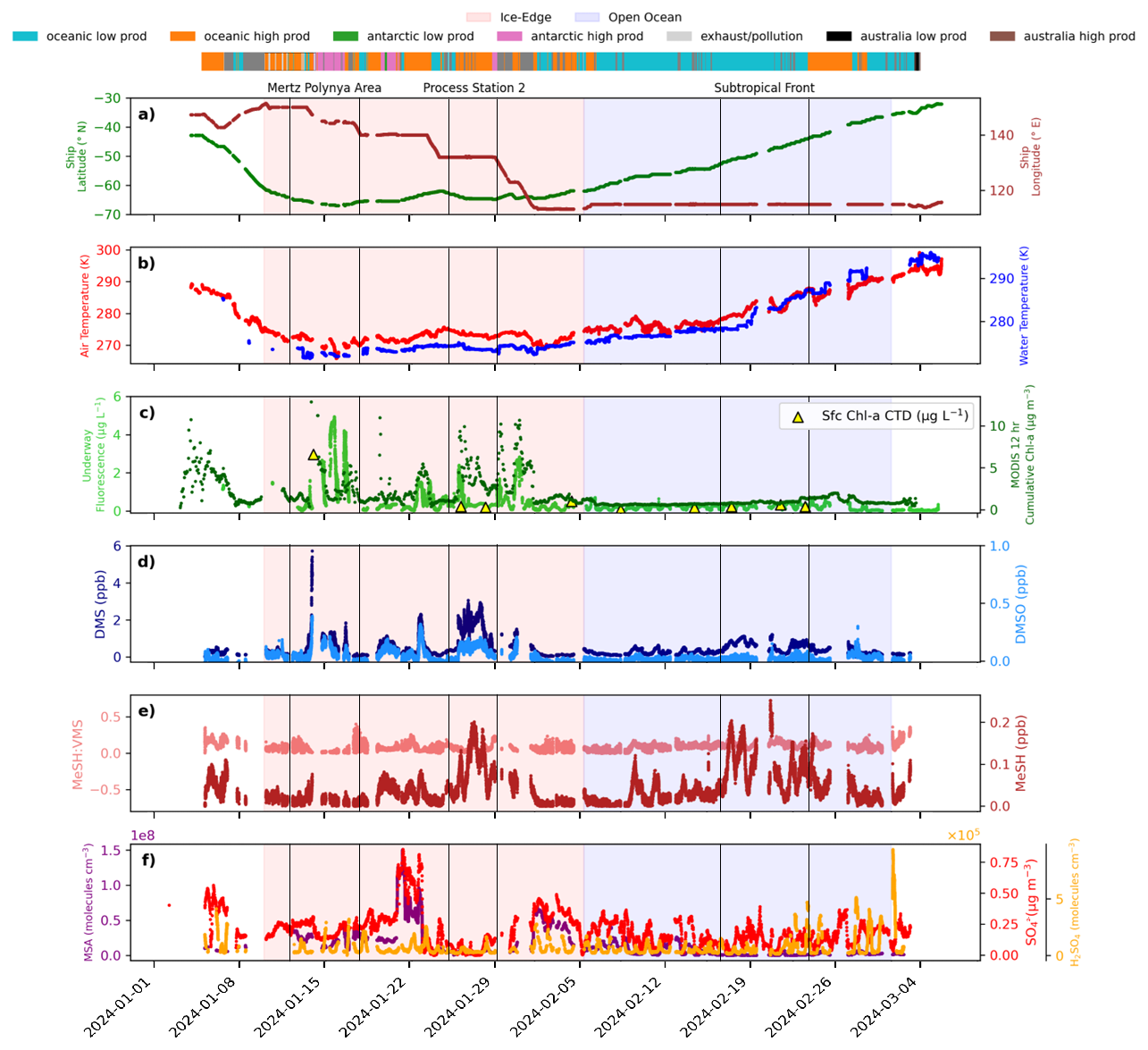
Figure 2 MISO voyage time series of in-situ measurements and derived product variables from satellite/model outputs. (a) RV Investigator ship latitude/longitude (green/brown), (b) RV Investigator measured air (red) and sea surface (blue) temperature, (c) MODIS 12 h cumulative Chl a (dark green), scaled underway in-situ fluorescence as a proxy for Chl a (light green) and surface layer HPLC Chl a concentrations collected from Conductivity, Temperature, and Depth instrument measurements (yellow triangles, left axis), (d) gas-phase volume mixing ratio DMS (navy) and DMSO (light blue), (e) gas-phase volume mixing ratio MeSH (dark red) and MeSH : VMS (light red), (f) gas-phase number density MSA (purple), sulfuric acid (orange) and aerosol-phase mass loading sulfate (red). The highlighted red section indicates the Antarctic Ice-Edge region and the blue section indicates the Open Ocean (I9S Transect) region. The colour bar at the top of the figure represents the air mass category based on coupled cumulative Chl a (a proxy for low/high biological productivity) and 12 h air mass backward trajectories. The colour bar also indicates data removed due to contamination from ship exhaust and transported pollution where the PTR-ToF-MS was usually changed to calibration and zero measurements (grey). Other breaks in the time series data indicate instruments were offline from ambient measurement or data were removed during quality control procedures. Black vertical lines indicate the periods of case studies discussed later in Sect. 3.4; Mertz Polynya Area, Process Station 2 and Subtropical Front.

3.2 Predictors of VMS Variability at the Antarctic Ice-Edge versus the Open Ocean

Next, we explore whether air mass history, in-situ observations, and trajectory-integrated metrics can explain and predict variability in VMS composition within Antarctic and oceanic air masses. A consistent co-varying relationship between DMS and cBLChl a occurred over the Antarctic Ice-Edge, which was especially driven by the oceanic high productivity air masses (R²= 0.49, n = 92, slope = 0.21, p< 0.01), as illustrated in Fig. 3. In fact, 6-hourly back trajectories demonstrated the strongest DMS–cBLChl a relationship in this region (Fig. S5); however, we use 12-hourly because it offers improved differentiation between Antarctic coastal and continental influence (Sect. 2.7). This DMS–cBLChl a coupling was significantly stronger than for DMS and measured in-situ Chl a (R²< 0.05). Likewise, for 12 h back trajectory averaged Chl a (R²< 0.1) and > 12 h back trajectory cumulative Chl a (R²< 0.2) over both transects.

At the Antarctic Ice-Edge, hyper-local and rapidly evolving phytoplakton blooms can develop over timescales of only 1–3 h, resulting in pronounced short-term variability in atmospheric VMS concentrations (Figs. 2 and 3). To more appropriately represent the spatial and temporal mismatch between measured atmospheric DMS concentrations and the underlying biogeochemical indicators integrated by the 12 h air mass back trajectories, atmospheric DMS concentrations were averaged from 1 to 5 h resolution (Fig. 3). This smoothing reduces the influence of transient local-scale variability while retaining the broader signal associated with air-mass exposure to the highly productive Antarctic coastal waters. Consistent with this interpretation, the relationship between DMS and cBLChl a strengthened following 5 h averaging (R² = 0.49) compared with the unsmoothed 1 h data (R²= 0.20). In contrast, no temporal smoothing was applied to the Open Ocean analysis because biological productivity was more spatially diffuse and less episodic. Under these conditions, 1 h atmospheric measurements combined with 24 h back trajectories provided the most representative relationship between DMS and cBLChl a (Fig. 3).

Given the abundance of high DMSP- and DMS-producing phytoplankton species and shallow MLDs encountered along the Antarctic coastal transect (Simó and Dachs, 2002), it is unsurprising we observed a close coupling between atmospheric DMS and cBLChl a in the high productivity Antarctic air masses (Sect. 3.2). Perhaps more notably, for the Antarctic coastal regions, cBLChl a, derived from monthly MODIS retrievals and 12 h back trajectories, was able to reproduce the time-varying behaviour of atmospheric DMS occurring on the order of hours (Fig. 3). Consistent with rapid DMS oxidation via OH-addition or bromine monoxide radical (BrO) oxidation at the Antarctic Ice-Edge (Fig. 1), DMSO strongly co-varied with DMS under this temperature regime (R²= 0.7, slope = 0.07, p< 0.01) and therefore was also tied to cBLChl a (R² = 0.29, n = 443, p< 0.01).

Despite the moderately strong correlation between atmospheric MeSH and DMS at the Ice-Edge (R²= 0.67, p< 0.001, using 5th–95th percentile data), MeSH did not show as close a relationship with cBLChl a (R²< 0.14; Fig. S8). Moreover, MeSH : DMS correlation was the same in both Antarctic high- and low productivity air masses, indicating that Chl a was not a common predictor of the coupling between MeSH and DMS at the Antarctic Ice-Edge. This is likely attributable to the dominance of heterotrophic processes involved in DMSP conversion to MeSH and not primary production, as is the case for DMS (Sect. 3.4, Figs. S4, S9, and S10). These findings indicate that, in the context of summertime ice-edge conditions, even low time resolution remote sensing ocean optical properties, used to construct our cBLChl a metric, may be a sufficiently robust predictor of atmospheric DMS emissions, but not for atmospheric MeSH emissions. This has the potential to significantly improve prediction of extreme atmospheric DMS dynamics, which remain a key challenge for polar sulfur chemistry models (Ishino et al., 2026).

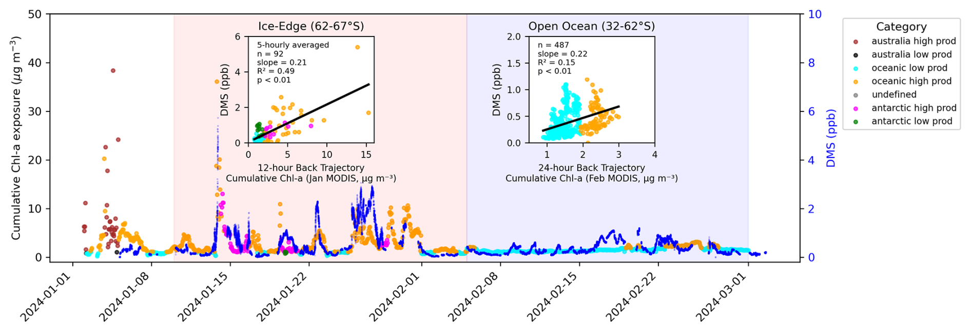
Figure 3 Time series of atmospheric DMS concentrations (blue data points), 12 h back trajectory cumulative boundary layer Chl a (January 2024 MODIS) over Antarctic Ice-Edge (red highlighted region) air mass history categories (coloured data points), and 24 h back trajectory cumulative boundary layer Chl a (February 2024 MODIS) over Open Ocean (blue highted region) air mass history categories. Regression scatter plots of DMS versus cumulative Chl a exposure are included over the Ice-Edge (left) and Open Ocean (right) periods. The Ice-Edge data points are averaged to 5-hourly resolution to optimise the regression, as the outliers significantly change the correlation in the 1-hourly data (see further in Sect. 3.4.)

Over high productivity regimes, other in-situ measurements and back trajectory variables including wind speed, air and sea surface temperature, humidity, total precipitation rate, ozone and boundary layer height, explained less than 20 % of the variance in DMS (Fig. S11). However, removing the biological source influence by analysing residuals after accounting for the cBLChl a resulted in in-situ wind speed explaining up to 36 % of the residual variance in DMS and up to 52 % of the residual variance in MeSH. Although a negative association between Chl a concentration and MLD was generally observed (Fig. S12), no direct linear relationship was identified between these variables within the high productivity regimes at the Antarctic Ice-Edge (R²< 0.07; Fig. S12). Neither was there a correlation between MLD (or Chl a : MLD) and DMS (R²< 0.05; Figs. S11, S12).

In contrast to the Antarctic Ice-Edge where cBLChl a was a reliable predictor of atmospheric DMS variability, cBLChl a was a poor indicator over Open Ocean regimes (Fig. 3), where the DMS–cBLChl a relationship was weaker (R² = 0.15, n = 487, slope = 0.22, p< 0.01) and an optimal relationship occurred using 24-hourly back trajectories (Figs. 3 and S5). North of the oceanic Polar Front, the absence of land barriers and the influence of the Antarctic Circumpolar Current create a more heterogeneous ocean surface with weaker, more dispersed, and often deeply mixed biological sources (Sokolov and Rintoul, 2007; Goosse et al., 2025). The dominant taxa are often weaker DMSP producers compared to polar bloom species (Teng et al., 2021; Asher et al., 2017), especially when compared to those observed at the Ice-Edge (Sect. 3.4). Relative to the shallower bathymetry and shallower MLDs in Antarctic shelf regions, such as the Mertz Polynya Area (MPA; 65.33–67° S, 140–150° E; see later in Sect. 3.4), where total Chl a consistently peaked and thus cBLChl a best predicted DMS (Figs. 3, S9 and S11; Sect. 3.4), MLDs over the Open Ocean were consistently deeper and phytoplankton biomass occurred at greater depths (Sect. 3.4; Fig. S4; i.e., 80 m along the I9S transect versus 5 m at the MPA). The MODIS Aqua satellite retrieves only near-surface concentrations of Chl a (NASA Earth Observations, 2025), and therefore may not accurately represent total phytoplankton biomass in the bulk water over the Open Ocean region (34–62° S).

The Open Ocean region was characterised by generally weak and inconsistent coupling between atmospheric VMS concentrations and the range of meteorological, oceanographic, and biological variables examined (Fig. S11). However, consistent with previous studies reporting the effect of open ocean slope transitions on biological sources (Shadwick et al., 2017; Hayward et al., 2024), Figure 4a illustrates that measured seafloor depth explained 35 % of the variance of our atmospheric VMS observations. The highest observed VMS concentrations occurred at the shallowest ocean depths (Fig. 4a), especially at the Subtropical Front (MeSH > 200 ppt and DMS > 1 ppb, < 4000 m; Figs. 2e and 4a). MLD exhibited a substantially stronger correlation with Chl a along the Open Ocean transect than at the Antarctic Ice-Edge (R² = 0.35; Fig. S12); however, no direct correlations were observed between MLD and DMS over the Open Ocean (R²< 0.01, p = 0.7; Fig. S12) or the Antarctic Ice-Edge (R² = 0.06, p< 0.01; Fig. S12). While we found that cBLChl a and MLD were moderately correlated over the Open Ocean (R² = 0.37), we did not observe a consistent relationship between these variables and atmospheric VMS (R²< 0.1; Fig. S11) unlike other previous research that has shown a correlation between seawater DMS and MLD as well as DMS and Chl a : MLD relationships (Simó and Dachs, 2002; Simó and Pedrós-Alió, 1999; McNabb and Tortell, 2023; Jarníková and Tortell, 2016). Despite this, we observed a moderately strong inverse relationship between VMS concentrations and measured bathymetry (R² = 0.35, Fig. 4), a pattern not observed over the region we define here as the Antarctic Ice-Edge. However, this relationship likely reflects the indirect influence of large-scale circulation and associated air mass history rather than a mechanistic control on VMS production or emission. Atmospheric factors that co-varied with VMS over the Open Ocean included ozone (Fig. 4b), relative humidity (Fig. 4c), back trajectory specific humidity, total precipitation rate and air temperature (Fig. S11), which together explained ∼ 25 %–50 % of the variance in VMS.

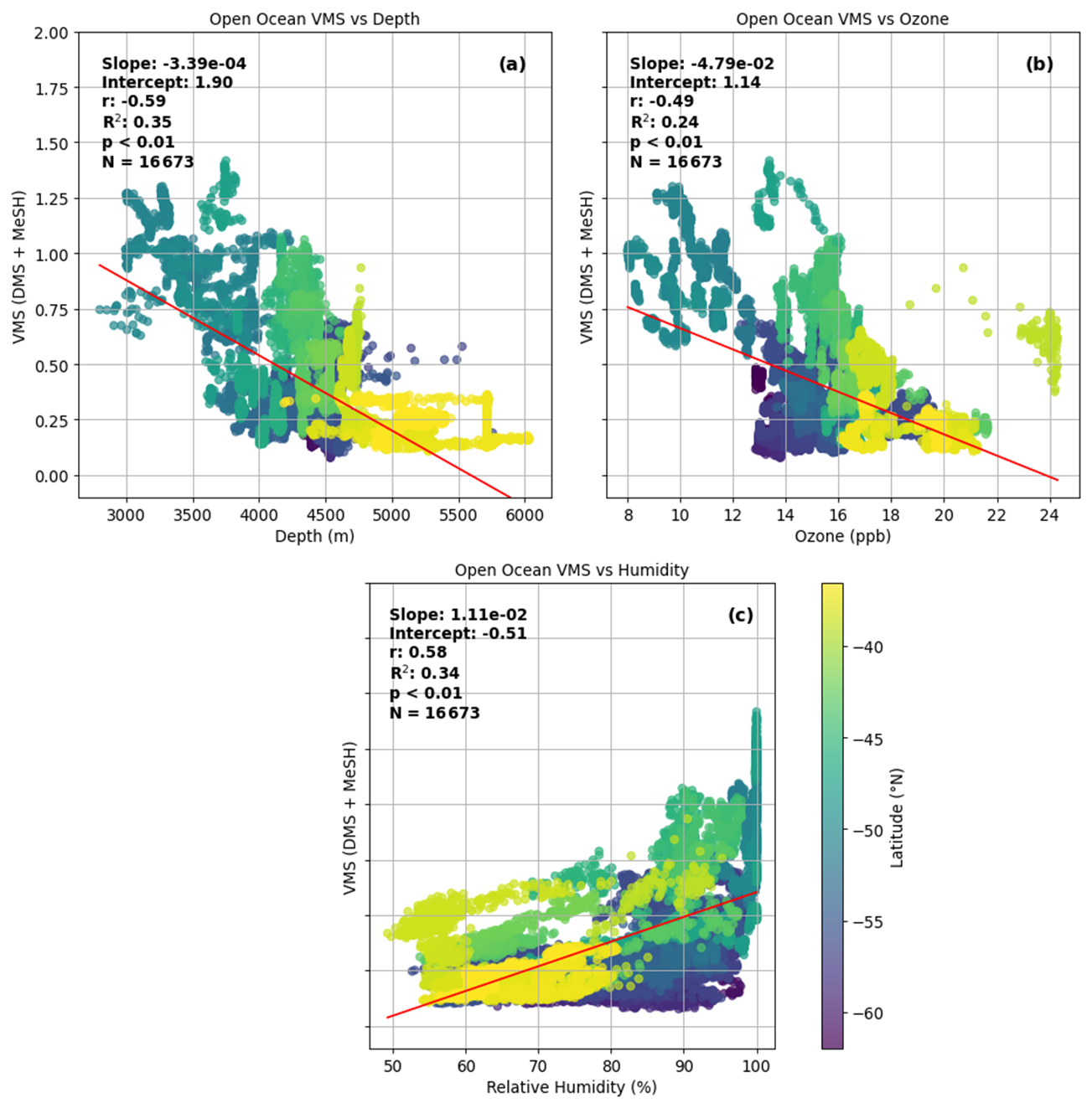
Figure 4 Atmospheric VMS relationships with ocean/seafloor depth (a), in-situ ozone (b), and in-situ relative humidity (c) over the Open Ocean region (34–62° S).

The absence of a robust predictor suggests that Open Ocean region atmospheric VMS variability emerges from the integration of heterogeneous source regions, transport, and atmospheric processing, rather than being governed by clearly identifiable source-related drivers like those observed at the highly biologically-mediated Antarctic Ice-Edge. Unlike the shallow, highly stratified polar waters, the deep offshore water column of the Open Ocean is shaped by large-scale oceanographic processes rather than local biological production, indicating it was not as strongly source-driven by local surface-ocean processes as what was observed at the Antarctic Ice-Edge. Along the I9S transect (115° E) measured during this voyage, previous work by McCartney and Donohue (2007) demonstrated that the water column is influenced by deep potential-vorticity maxima and enhanced mixing where dense western-boundary waters interact with lighter Antarctic Circumpolar Current waters.

3.3 Spatial Variability in Atmospheric MeSH : DMS Ratios

Spatial patterns in the atmospheric MeSH : DMS ratio provide insight into how underlying DMSP cycling and atmospheric processing modulate VMS speciation across the Southern Ocean regimes. As first presented in Mynard et al. (2025b), atmospheric MeSH : DMS ratios showed pronounced spatial variability, with lower and more variable ratios observed along the Ice-Edge (∼ 0.05) than over the Open Ocean (∼ 0.15), and lower than previously reported from other Southern Ocean data sets collected at lower latitudes (∼ 0.13–0.19; Lawson et al., 2020; Rocco et al., 2025). The low atmospheric MeSH : DMS ratios that we measured at the Antarctic Ice-Edge are more consistent with ratios of ∼ 0.02 reported from measurements of dissolved MeSH and DMS in coastal waters west of the Antarctic Peninsula (Berresheim, 1987), and median atmospheric ratios < 0.1 reported from Northern Hemisphere high latitudes (Ishino et al., 2026). These lower and more variable MeSH : DMS ratios may have implications for modelling studies which have used global seawater DMS climatologies and the relationship between MeSH and DMS to construct estimates of oceanic MeSH (Tashmim et al., 2025; Wohl et al., 2024; Jacob et al., 2026). These modelling studies have used MeSH : DMS ratio scaling factors on the order of 0.1–0.2, which likely resulted in an overestimation of MeSH emissions for regions such as the Antarctic Ice-Edge.

In contrast to the air masses encountered at the Antarctic Ice-Edge, the Open Ocean air masses exhibited a consistent coupling between DMS and MeSH (as first described by Mynard et al., 2025b), yet their distributions are largely decoupled from surface chlorophyll biomass (Figs. 3 and S11). This is because DMS and MeSH largely share a common biogenic origin from marine DMSP cycling and experience relatively homogeneous atmospheric processing. At the Antarctic Ice-Edge, the MeSH : DMS relationship is more complex, as discussed in the next Sect. 3.4.

The atmospheric MeSH : DMS ratios observed over the Open Ocean (∼ 0.15) in this study are consistent with the 0.13–0.19 ratios reported from other Southern Ocean data sets collected at lower latitudes (Lawson et al., 2020; Rocco et al., 2025; Mynard et al., 2025b) and the ∼ 0.1–0.2 ratios reported from other ocean regions (Novak et al., 2022; Tashmim et al., 2025; Wohl et al., 2025; Kilgour et al., 2025). We estimated sea–air fluxes of DMS and MeSH from their nocturnal accumulation in the marine boundary layer following Marandino et al. (2007); Lawson et al. (2020); Rocco et al. (2025) (see detailed method in Sect. S4). This approach exploits reduced nighttime photochemical loss, allowing DMS and MeSH to accumulate in the boundary layer and providing an estimate of their net oceanic emissions. Consistent with this coupling under low-productivity conditions (where cBLChl a does not dominate variability in this study), nocturnal accumulation periods over the Open Ocean yielded sea–air flux estimates of 15–124 for DMS and 0.1–17 ng m⁻² s⁻¹ for MeSH (Sect. S4; Tables S1 and S3), with a broadly variable MeSH : DMS flux ratio (0.008–0.462) that generally exceeded recent southwest Pacific nocturnal accumulation estimates (Lawson et al., 2020; Rocco et al., 2025). However, the increase in atmospheric MeSH : DMS with increased SSTs observed in this study, especially over the Subtropical Front (Fig. S13), is not consistent with the trend determined in a previous global synthesis of seawater MeSH and DMS concentrations (Wohl et al., 2024), which reported lower MeSH : DMS ratios (∼ 0.1) associated with SSTs above a threshold of 8–12 °C, and higher MeSH : DMS (∼ 0.3) at lower SSTs; nevertheless, that analysis was based on very limited data from these latitudes of the Southern Ocean.

3.4 Case Studies of Enhanced VMS: Biological Drivers and Speciation

Having identified the spatial patterns in atmospheric DMS and MeSH concentrations and the key predictors of their variability across the Antarctic Ice-Edge and Open Ocean regions, we now investigate selected case studies to gain process-level insights into how Southern Ocean and Antarctic coastal oceanographic and biological features influence atmospheric DMS and MeSH production and emission. Extreme seawater DMS concentrations, in excess of 100 nM, have been reported in Antarctic coastal waters associated with springtime sea ice break up that releases trapped DMS/P and seeds subsequent intense phytoplankton blooms that can persist throughout the summer (Webb et al., 2019; Stefels et al., 2018; Trevena and Jones, 2006). The spatial and temporal heterogeneity in VMS emissions introduced by these hotspots is not well represented in models, which instead often implement open ocean derived fluxes (Ishino et al., 2026). Furthermore, current models do not account for MeSH, which growing evidence suggests also plays an important role in aerosol formation and the oxidative capacity of the atmosphere (Novak et al., 2022; Wohl et al., 2024). Modelling efforts to date have exploited the typically close coupling between DMS and MeSH to derive global MeSH emission fields from DMS climatologies (Wohl et al., 2024; Tashmim et al., 2025; Jacob et al., 2026). However, as mentioned above, although the MeSH : DMS ratios over the Southern Ocean are relatively consistent (10 %–35 %), they vary seasonally and are much lower (< 5 %) and more variable at the Antarctic coast (Mynard et al., 2025b).

We observed two distinct episodes at the Antarctic coast with extreme atmospheric VMS concentrations, up to 25 times the MISO voyage medians, which were associated with oceanic and Antarctic high productivity air masses sampled over intense blooms at the Mertz Polynya (MPA), and at a process station (PS2) along the continental slope. In both case studies, atmospheric concentration dynamics were predominantly source driven, rather than significantly controlled by atmospheric loss processes. This is supported by the close coupling between air mass DMS concentrations and exposure to phytoplankton biomass as indicated by monthly MODIS Chl a (Fig. 3) along with the high dissolved concentrations of DMS at the MPA (Fig. S3; dissolved DMS measurements were not available at PS2). Wind speeds and water temperatures in both case studies were not outside of normal ice-edge conditions (Figs. 2 and S14), suggesting that high atmospheric VMS concentrations and concentration ratios are therefore considered indicative of water-side processes. A third period of atmospheric VMS enhancements occurred at the biologically productive Subtropical Front region.

3.4.1 The Mertz Polynya Area (65.33–67° S, 140–150° E)

The first extreme event occurred over 12–17 January 2024, with atmospheric DMS concentrations up to 5.7 ppb (>q 95), with associated MeSH concentrations of 90 ppt and exhibited moderately strong MeSH : DMS relationships (R² = 0.58) yet a very low MeSH : DMS of 0.4 %. These air masses were of mixed oceanic and Antarctic high productivity origins that had recently passed over the intense phytoplankton blooms in the Mertz Polynya Area (MPA; 65.33–67° S, 140–150° E). The MPA is a shallow, stratified, post-calving polynya system where enhanced light exposure and sea-ice circulation support intense phytoplankton blooms even in late summer (Shadwick et al., 2017). This East Antarctic polynya system has been the subject of recent dramatic changes in dynamics and biogeochemistry following the 2010 calving of the Mertz Glacier Tongue (Shadwick et al., 2013). In November 2023, sea-ice extended to ∼ 63° S covering most of the MPA before retreating through December and the subsequent melt exposed the MPA in January 2024 shortly before the MISO voyage (MODIS Aqua, Fig. S15). During MISO, the RV Investigator transited across the Antarctic continental shelf and shelf-edge within the MPA, where the deep Southern Ocean (> 3000 m) transitioned to the shallow (200–1000 m) shelf waters (Fig. S9). The highest atmospheric DMS concentrations coincided with the Antarctic shelf-edge region, which is recognised as a zone of enhanced biological productivity and extremely high DMS fluxes (Webb et al., 2019; Stefels et al., 2018). Surface waters in this region were characterised by decreased salinity (33.8 PSU) and sub-zero temperatures (<−1 °C). Depth profiles of temperature and salinity from CTD sampling showed a very shallow surface MLD of ∼ 10 m (Fig. S4). Based on MODIS Chl a the MPA bloom intensified during January and dissipated by late February (Fig. S15). The ship was stationary for 3 d close to a summer retreating sea ice region of very high biological productivity. Chl a from in-situ surface fluorescence measurements was up to 5 µg L⁻¹ (Fig. 2). Laboratory pigment analysis from CTD vertical profile sampling showed a ∼ 3 µg L⁻¹ Chl a band extending from the surface to ∼ 30 m depth (Fig. S4a). Within the surface to 30 m, phytoplankton community composition as a fraction of Chl a showed a high abundance of haptophytes (3 × median) and dinoflagellates (5×median), known strong DMS/P producers (Figs. S3 and S4). Diatoms were the dominant phytoplankton class (32×median), which in high abundance can also be important dissolved DMS/P producers in sea ice regions (Sheehan and Petrou, 2019). This period also coincided with high dissolved DMS/P concentrations (> 100 nM, Fig. S3) and elevated seawater DMSO (> 10 nM) which correlated strongly with seawater DMS (R² = 0.78, p< 0.01, n = 35). Chromophoric dissolved organic matter (CDOM) was low at the surface (< 1.5 ppb), but increased to > 2 ppb below ∼ 100 m depth (Fig. S10). Low levels of CDOM may imply less DMS loss via both CDOM-mediated photolysis (Taalba et al., 2013) and lower bacterial DMS consumption (Piontek et al., 2021).

The shallow mixed layer, very high biological productivity, and elevated light conditions experienced at the MPA likely favoured direct DMS production by phytoplankton, especially haptophytes such as Phaeocystics sp., and explains the close coupling between DMS and air mass cumulative Chl a exposure in this region (Stefels and van Boekel, 1993; Simó and Pedrós-Alió, 1999; Teng et al., 2021; Sun et al., 2016; van den Berg et al., 1996). DMSO reduction may have been an additional important pathway of DMS production at the MPA. Seawater dissolved DMSO is produced primarily through the photochemical and biological oxidation of DMS (Spiese et al., 2009; Brimblecombe and Shooter, 1986; Hopkins et al., 2023) and, to a lesser extent, via direct release from DMSP-containing phytoplankton, such as dinoflagellates, diatoms and haptophytes (Simó et al., 2000, 1998). High concentrations of dissolved DMSO observed near the Antarctic coast (Fig. S3) have also been observed elsewhere in Antarctic waters (Trevena and Jones, 2006; Tison et al., 2010), associated with the haptophyte Phaeocystis antarctica. Although primarily recognised for its high DMSP production, P. Antarctica has also been reported to contain and release DMSO (Asher et al., 2011, 2017). While substantial DMSO production is more commonly attributed to oxidative and microbial processes (Spiese et al., 2009), Asher et al. (2011) showed that intense microbial activity in Antarctic sea-ice environments promotes significant DMS production via rapid DMSO reduction and DMSP cleavage, suggesting that this rapid biological DMSO reduction can dominate DMS production across diverse Antarctic sea-ice environments.

The overall biological pathways driving phytoplankton production of DMS/P/O are considered to be at least partly driven by physiological stress where phytoplankton may produce DMS/P/O as a cryoprotectant, osmoregulator, or in response to oxidative stress (Vance et al., 2013; McNabb and Tortell, 2025; Kirst et al., 1991). It is plausible the production of these sulfur species was upregulated in the prevailing conditions at the MPA where the spring/summer sea-ice retreat results in rapid changes in temperature, UV, salinity and nutrient availability. Polar diatoms in very high abundance, as was the case for the MPA (Fig. S4c), are typical of summertime blooms in this region and can also significantly contribute to the pool of DMS/P (Sheehan and Petrou, 2019). It is also possible sea-ice algae and their DMS/P/O metabolites further added to the DMS pool at the MPA during the January sea-ice retreat (Tison et al., 2010). However, the open water conditions during sampling and the close coupling between MODIS Chl a and DMS observed suggest that while sea-ice algae may have seeded the blooms encountered during MISO, in-situ production via the aforementioned pathways were the dominant source of enhanced DMS observed at the MPA. The very low MeSH : DMS ratio of 0.4 % at the MPA compared to ∼ 15 % over the Open Ocean is largely due to the very intense DMS emissions, but may also be a consequence of the shallow MLD resulting in UVB-photoinhibition of heterotrophic bacterioplankton and lower bacterial sulfur demand limiting MeSH production (Simó and Pedrós-Alió, 1999).

3.4.2 Process Station 2 (64° S, 132° E)

A second episode during the period 26–29 January 2024, referred to here as Process Station 2 (PS2), was characterised by high atmospheric mixing ratios of both DMS (up to 3.1 ppb, >q 90) and MeSH (up to 200 ppt, >q 95) (MeSH : DMS = 3 %). PS2 occurred when the ship was stationary to the north-west of the MPA (64° S, 132° E) in a deeper (> 1500 m), warmer (> 0 ° C) open-ocean region over the continental slope (see Fig. S9). Depth profiles of temperature and salinity from CTD sampling showed a moderately shallow mixed layer ∼ 17 m (Fig. S4). The sampled air masses were predominantly easterly, traversing biologically productive pelagic and Antarctic coastal regions for extensive periods during 26–27 January. This period was characterised by cloudy conditions (low photosynthetically active radiation) and rainfall (Fig. S14), which may have limited photo-inhibition of bacterioplankton resulting in slightly higher atmospheric MeSH concentrations associated with air masses from this region compared to the MPA. Note that the rapid increase in atmospheric DMS (∼ 3 ppb) and MeSH (∼ 100 ppt) around 22–23 January 2024 (Fig. 2) occurred when air masses were directly downwind of the biologically productive PS2 region. The PS2 region had lower surface Chl a compared to the MPA from in-situ surface fluorescence measurements (up to 2 µg L⁻¹). CTD depth profiles showed an increase in Chl a from 0.2 µg L⁻¹ at the surface (5 m) to a peak of 0.65 µg L⁻¹ at ∼ 55 m depth (Fig. S4). MODIS Chl a indicated that the bloom persisted throughout February (Fig. S15). Haptophyte abundance in the sub-surface bloom at PS2 was lower than at the MPA (0.1 compared to 0.25 µg L⁻¹ Chl a) but higher than non-bloom Antarctic coastal regions (∼ 0.05 µg L⁻¹ Chl a) and haptophytes represented a higher proportion of total Chl a (Fig. S4). The PS2 bloom had a higher abundance of dinoflagellates than the MPA (0.22 versus 0.07 µg L⁻¹ Chl a) as well as significantly lower fraction of diatoms compared to the MPA (0.3 compared to 2.5 µg L⁻¹ Chl a). Dissolved DMS/O/P concentrations were not available for this region. Potentially indicative of a more heterotrophic phase and downwelling at the shelf was the consistently higher pCO₂ (∼ 350 ppm) compared to the MPA (∼ 208 ppm), lower O₂ saturation (< 100 %) (Fig. S9), and higher CDOM (2–3 ppb throughout the measured water column ∼ 0–200 m; Fig. S10). A 1000 L sample of natural seawater was collected at PS2 in deckboard 2000 L mesocosm tanks and incubated over 10 d (Sect. S5). The mesocosm headspace concentration of MeSH exhibited significant diel variability on the order of 10s of ppt with maxima in low light conditions; whereas DMS showed little diurnal variability with the most significant changes occurring on the order of days (Fig. S16), providing further evidence of the photo-inhibition effect with higher MeSH associated with low light conditions.

Heterotrophic dinoflagellates can also play a key role in phytoplankton herbivory in coastal Antarctic waters (Archer et al., 1996), and the higher abundance of dinoflagellates at PS2 (Fig. S4d) may have contributed to higher heterotrophy in this region. The lower proportion of diatoms and higher proportion of haptophytes to total Chl a at PS2 compared to the MPA (Fig. S4) may be indicative of grazing by Antarctic krill, which are known to congregate near the Antarctic continental slope (Freer et al., 2025) and prefer large diatoms, leaving small cells such as haptophytes behind, either due to selective feeding or the inefficient filtering of small cells with the feeding apparatus (Heidemann et al., 2024). Krill grazing may have a large influence on ocean biogeochemistry through pathways such as sloppy feeding and the production of faecal pellets, with associated organic material subject to bacterial remineralisation (Cavan et al., 2019). Such processes have been shown to result in increased dissolved-phase DMSP (Kasamatsu et al., 2004), which is required for the demethylation/demethiolation pathway to proceed to MeSH production (Fig. 1; Hopkins et al., 2023). We therefore postulate that the heterotrophic characteristics at PS2 were conducive to enhanced MeSH production independent of chlorophyll biomass (Kiene et al., 1999; Hopkins et al., 2023), and may explain the increased MeSH atmospheric concentrations at PS2 compared to the MPA.

3.4.3 Subtropical Front Region (42–52° S)

The highest atmospheric MeSH concentrations (up to 252 ppt) were observed over subantarctic waters between ∼ 42–52° S along the northward I9S Transect bounded by the Subtropical Front (16–23 February 2024; Fig. 2). DMS was also elevated in this region (up to 1.37 ppb) and closely coupled with MeSH (R² = 0.72) with a MeSH : DMS ratio of ∼ 0.15 (Fig. S13). Underway SST and salinity data showed a step change from < 6 °C at 51° S to > 10 °C at 49° S and salinity 33.9 to 34.3 PSU (Fig. S4). Depth profiles of salinity and temperature indicate a shallower MLD of ∼ 50 m formed between 46–35° S (Fig. S4). The air masses sampled in this region were predominantly from the WNW and were mostly classified as oceanic low productivity. However, air mass back trajectories combined with MODIS cBLChl a indicate air masses with the highest VMS concentrations passed over a wide band of biological productivity between 44–36° S (Fig. S4). Underway surface Chl a fluorescence was low (< 1 µg Chl a L⁻¹) until around 48° S where it increased up to 2 µg Chl a L⁻¹ at ∼ 43° S. Depth profiles showed pronounced fluorescence within the MLD at 50–35° S with a high abundance of haptophytes (20 %–50 % of total Chl a; Figs. S3, S4) in subantarctic waters between 50–43° S.

Coccolithophores and Phaeocystis sp. are the dominant genus of haptophytes in this region and these strong DMS/P producers are considered to be major contributors to the elevated seawater and atmospheric DMS/P observed during summer and autumn in subantarctic waters (Curran et al., 1998; McTaggart et al., 1995; Keller et al., 1989; Nissen et al., 2018). Enhanced atmospheric VMS and higher MeSH : DMS ratios have previously been reported over a coccolithophore-rich bloom in the Southwest Pacific Ocean (Lawson et al., 2020). Conversely, cooler waters (< 6 °C) south of 50° S in this study were dominated by diatoms, which produce less DMSP (Figs. S3, S4). A range of environmental factors including temperature, light, MLD, nutrient availability (particularly diatom-limiting silicic acid), as well as zooplankton grazing, are key factors controlling haptophyte and diatom populations, and therefore VMS emissions, in this region (Oliver et al., 2023; Nissen et al., 2018). Similarly to the sea ice region described above, rapid changes in temperature, salinity, MLD and nutrient availability along the subtropical frontal region may have resulted in an upregulation of DMS/P production as a stress response within the haptophyte assemblages present. In addition, higher cloud and rainfall conditions in this sampling period (Fig. S14) may have limited photo-inhibition of bacterioplankton resulting in the higher atmospheric MeSH concentrations associated with air masses from this region. Given its large spatial extent, this frontal band of elevated biological activity, and higher MeSH : DMS ratios (∼ 0.15) compared to the Antarctic Ice-Edge (∼ 0.05), indicates that these latitudes of the Southern Ocean could be an important regional and global source not only for DMS but also MeSH.

In summary, the underlying biological and oceanographic conditions observed during the case studies of VMS enhancements presented here for the Ice-Edge (MPA, PS2) and near the Subtropical Front (42–52° S) demonstrate strong controls on the abundance and speciation of atmospheric VMS. In particular, haptophyte abundance appears to be a key biological driver of marine DMS/O/P production. Furthermore, we hypothesise that heterotrophic processes, such as zooplankton grazing and bacterial catabolism controlled the relative MeSH : DMS yields within the surface ocean.

Taken together, these regime-dependent responses between Antarctic Ice-Edge and Open Ocean regions demonstrate that empirical relationships between biogeochemical properties, VMS, and MeSH : DMS cannot be applied uniformly across the Southern Ocean. Instead, they underscore that Southern Ocean phytoplankton dynamics and associated sulfur cycling emerge from the interaction of multiple environmental drivers (temperature, light, and MLD across fronts), which organise distinct vertical biomass and community compositions in ice-edge versus offshore systems (Thomalla et al., 2023). In ice-edge regimes, intense, spatially coherent surface blooms under shallow stratification and episodic nutrient supply can link surface Chl a more directly to atmospheric VMS emissions; whereas in offshore regions, weaker, more deeply mixed, and spatially sparse biological activity decouples surface Chl a from atmospheric VMS. Our results show that predictive frameworks for DMS and MeSH contributions to the total Southern Ocean VMS burden must be explicitly aware of regional differences in physical–biogeochemical regimes and the influence of air mass history.

3.5 First Generation Oxidative Fate of DMS

Once emitted into the atmosphere, gas-phase oxidation and multiphase chemical processing are important loss mechanisms for VMS (Fig. 1), which contribute to the atmospheric sulfur cycle and to Southern Ocean aerosol and cloud processes (Charlson et al., 1987; von Glasow and Crutzen, 2004; Carslaw et al., 2013). In the cloud-free marine boundary layer, DMS is oxidised to DMSO, mainly via oxidation by OH-addition and BrO (Fig. 1; Hoffmann et al., 2016). BrO oxidation has previously been identified as a potentially important mechanism, contributing up to 44 % of global DMSO production in a modeled global tropospheric DMSO budget (Chen et al., 2018). MeSH is primarily oxidized via H-abstraction to short-lived radicals and SO₂ (not measured on MISO), and apart from acting as an OH-scavenger, MeSH oxidation would not contribute to the observed atmospheric DMSO abundance (Novak et al., 2022; Wohl et al., 2024). Observed DMS and DMSO concentrations are well correlated at the Ice-Edge (R² = 0.69, p< 0.01) but weakly correlated over the Open Ocean (R² = 0.04, p< 0.01). The DMSO : DMS ratio varied significantly (∼ 0–1) with temperature across spatial regions of the Southern Ocean (Fig. 5).

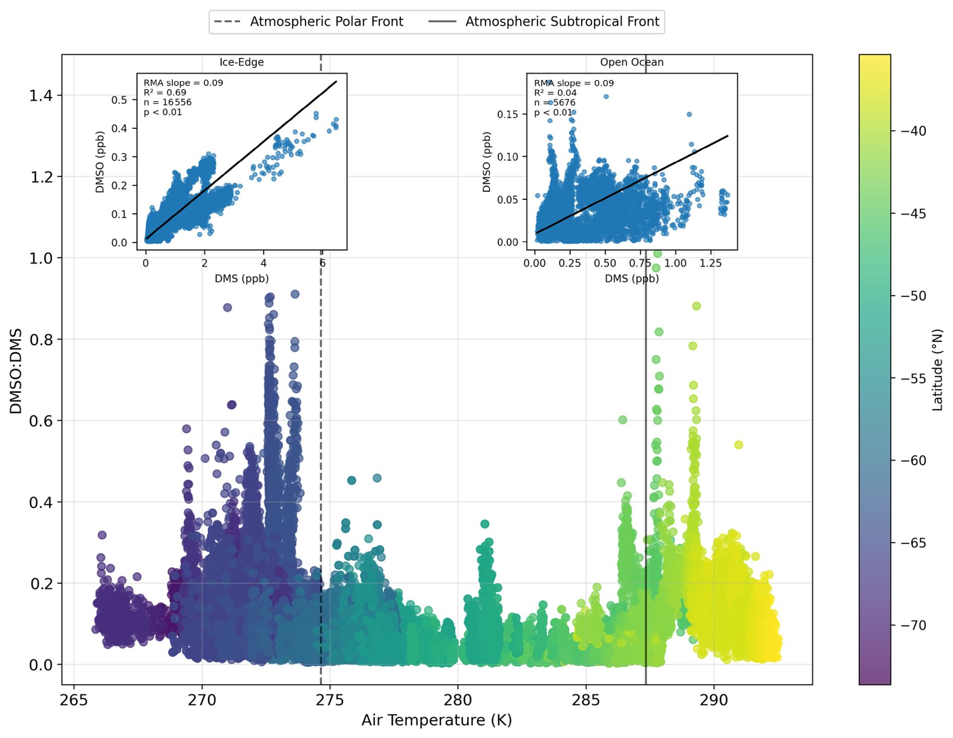
Figure 5 Atmospheric DMSO : DMS ratio across measured air temperatures. Latitudes south of the atmospheric Polar Front (< 62° S, dashed line) are considered Ice-Edge with associated DMSO : DMS RMA scatter plot (top left), and north of the atmospheric Polar Front (> 62° S) spanning the Southern Ocean and the atmospheric Subtropical Front (∼ 40–50° S, solid line) are considered Open Ocean with associated DMSO : DMS RMA scatter plot (top right).

South of the atmospheric Polar Front, subzero air temperatures coincide with elevated DMSO : DMS and a strong coupling (R² = 0.69, Fig. 5), consistent with previous work highlighting temperature-driven partitioning of DMS oxidation products near Antarctica (Berresheim and Eisele, 1998; Davis et al., 1998; Legrand et al., 2001). We propose that the strong DMSO : DMS coupling at the Ice-Edge could be evidence of local, rapid OH-addition oxidation of DMS in the photochemically active boundary layer of the summertime Antarctic Ice-Edge. This pathway may be amplified by BrO-mediated oxidation, which has reaction rates an order of magnitude faster than OH-mediated oxidation in the Antarctic environment, leading to estimated DMS lifetimes on the order of minutes to hours (Saiz-Lopez et al., 2007; Mynard et al., 2025b; Davis et al., 1998) which is consistent with the observed DMSO : DMS correlation at the Ice-Edge (Fig. 5). The DMSO : DMS correlation is even stronger and an increased slope is observed (R² = 0.76, slope = 0.16, p< 0.01; Fig. S17) when only considering intense sunlight conditions (PAR > 85th percentile: > 700 µmol m⁻² s⁻¹) and low-moderate in-situ wind speeds (1–10 m s⁻¹), suggesting that under such conditions local photochemical production of DMSO from DMS likely occurred at the Ice-Edge. This is further supported by the absence of any significant time lag in the time-varying behaviour of the two species. An autocorrelation analysis shows that they are optimally coupled at the time of measurement, with no improvement in the correlation when time-lagging the data (Fig. S18). Although these are likely significantly influenced by meteorology, the lack of observable lag under stable low wind speed conditions points to the importance of oxidation mechanisms, which occur faster than characterized reactions between DMS and OH. However, co-emission of DMSO and DMS from the surface ocean could, in theory, also explain the lack of lagged time varying behaviour.

DMSO is highly soluble in seawater, with a Henry's law constant 5 orders of magnitude lower than that of DMS (Dacey et al., 1984; Watts and Brimblecombe, 1987). Its ventilation from seawater is therefore not thermodynamically favoured. This is supported by observations during on board mesocosm incubation experiments which were conducted along the Antarctic Ice-Edge (Sect. S5). In these experiments, DMS concentrations reached as high as 15 ppb (∼ 2–3 times the median ambient concentrations) within the oxidant-free mesocosm headspace, while DMSO had a maximum atmospheric concentration of 40 ppt, it was rarely observed above detection limits in the headspace, and did not co-vary with DMS. This is also consistent with Kilgour et al. (2022) who studied an induced phytoplankton bloom and found little evidence for ventilation of DMS oxidation products into oxidant-free headspace environments. Therefore, multiple lines of evidence point to gas-phase production of DMSO from DMS oxidation pathways rather than ventilation from the ocean surface as the dominant source of DMSO.

However, in addition to microbial degradation and ventilation to the atmosphere, DMS is also lost from the surface ocean via photolysis (Galí et al., 2023). This process occurs in the upper mixed layer when DMS is oxidised by reactive species generated from light absorption by photo-active substances, particularly CDOM and nitrate, with peak photolysis at UV wavelengths ∼ 320–330 nm, yielding DMSO as the main product (Brimblecombe and Shooter, 1986; Galí et al., 2016). The mesocosm setup used in the experiments (Sect. 3.4; Fig. S16) filtered out UV wavelengths < 364 nm. Overall, DMS loss via photo-oxidation has been shown to be particularly important in the Southern Ocean (Galí et al., 2023) and potentially responsible for the decoupling observed between DMS and Chl a in frontal regions exhibiting high CDOM and nitrate concentrations (McNabb and Tortell, 2023). It is unclear if DMSO produced at the air-sea interface can be efficiently transferred to the atmosphere; however, it may provide another possible explanation for the tight DMS : DMSO coupling observed in the DMS hotspots encountered along the Ice-Edge in this study.

We found no consistent correlation between any of the VMS species (DMS, MeSH, and DMSO) and any of the later VMS oxidation products measured during the MISO voyage, namely MSA (g), SA (g), or aerosol-phase sulfate (all R²< 0.2; see Fig. S11). This decoupling is likely indicative of the importance of multiphase chemistry, meteorology, and sinks in the atmospheric concentrations of later VMS oxidation products, and is consistent with other studies of atmospheric sulfur in remote marine atmospheres (Read et al., 2008; Zhang et al., 2024; Shen et al., 2022; Chen et al., 2012). Persistent low-pressure systems and cyclones around the Antarctic continent promote strong vertical uplift, shifting much of the MSA and SA production into the free-troposphere where low temperatures and low condensation sink favour slower, multistep oxidation pathways and new particle formation. Recent work by Miljevic et al. (2025) suggests that katabatic outflow transports free-tropospheric, highly acidic aerosol particles back into the boundary layer, where low RH and high acidity can drive evaporation of particle-phase MSA, which helps to explain the decoupling between our observed MSA/SA from local VMS emissions.

As illustrated in Fig. 5, the DMSO : DMS ratio is significantly and consistently higher under the cold conditions of the Ice-Edge below the atmospheric Polar Front (median DMSO : DMS = 12 %) than in Open Ocean conditions between the polar and subtropical fronts (median DMSO : DMS = 5 %). A significant potential contributor to this dynamic is likely the temperature dependence of DMS oxidative pathways, illustrated in Fig. 1. As described in Berresheim and Eisele (1998), at low temperatures (< 285 K) the OH addition pathway is favoured, leading to higher production of DMSO and MSA. Under warmer conditions however, the H-abstraction DMS oxidation pathway is more favoured, which would lead to lower yields of DMSO and higher yields of SO₂ and SA. While the transition from a low to high DMSO : DMS regime occurs at significantly less than 285 K and synoptic scale dynamics related to DMS lofting above the boundary layer have also been identified as important contributors to DMSO production (Nowak et al., 2001; Jourdain and Legrand, 2001), the temperature dependence of oxidative fate remains an important likely contributor to observed dynamics. As the air temperature increases north of the atmospheric Polar Front and over the Open Ocean, we find that DMSO : DMS generally decreases and they become decoupled (R² = 0.04, Fig. 5). This is consistent with austral summer DMSO measurements conducted at a similar latitude at Amsterdam Island (37.83° S, 77.50° E; Sciare et al., 2000), which found that DMSO co-varied with DMS but they were only moderately correlated (R² = 0.21). Our current temperature-dependent conceptual framework for VMS oxidation does not fully capture the observed behaviour of an increased DMSO : DMS ratio at the warmer Subtropical Front (42–52° S, Fig. 5). This suggests that latitudinal temperature gradients may not always be the primary factor responsible for DMSO : DMS variability across the broad regions of the Southern Ocean, although the mechanistic processes underlying this remain insufficiently understood and unresolved.

4 Conclusions

This study reveals that controls on atmospheric volatile methylated sulfur compounds (VMS) are highly regionally dependent, shaped by distinct biological regimes along the Antarctic Ice-Edge and by physical and meteorological drivers over the Open Ocean. At the Ice-Edge, extreme DMS episodes were tightly linked to recent ice-edge productivity, shallow mixed layers and high haptophyte contributions to total Chl a, establishing monthly MODIS Chl a coupled with modelled air mass back trajectories as a robust proxy for DMS source strength; but a poor proxy for MeSH, which was associated with heterotrophic activity and photo-physical conditions. Furthermore, DMS was a less reliable predictor of MeSH under these high productivity, heterogeneous Antarctic coastal conditions. Given the very low MeSH : DMS ratios observed at the ice-edge in this study (< 3 %), approaches that infer MeSH fluxes and atmospheric abundances by scaling from DMS climatologies, as implemented in recent models (Wohl et al., 2024; Tashmim et al., 2025; Jacob et al., 2026), are likely to substantially overestimate MeSH contributions over this Antarctic coastal region.

North of the Polar Front, where biological sources are weaker and more deeply mixed, VMS variability was governed primarily by physical ocean structure, boundary-layer dynamics, humidity, air temperature and oxidant availability. In the Open Ocean, the lack of a robust predictor indicates that atmospheric VMS variability reflects the integrated effects of heterogeneous source regions, transport, and atmospheric processing, rather than clearly identifiable source-related drivers like those observed at the highly biologically mediated Antarctic Ice-Edge. Consistent with this, relationships with individual physical variables (e.g., mixed layer depth and bathymetry) likely capture the indirect influence of large-scale circulation, rather than a mechanistic control on VMS production or emission. While DMS and DMSO were strongly coupled at the Antarctic Ice-Edge, later oxidation products (MSA and SA) were further decoupled from their VMS precursors, reflecting the dominant influence of temperature-dependent pathways and air mass history.

Together, these findings underscore that Antarctic VMS cannot be represented by biological proxies alone. Accurate prediction of sulfur emissions and their contribution to aerosol requires frameworks that couple ocean biogeochemistry with boundary-layer transport and temperature-dependent oxidation. While these are being rapidly introduced into Earth System Models, explicitly resolving all relevant processes in fully coupled biogeochemistry–ocean–atmosphere simulations currently remains computationally impractical on climate-relevant timescales (Bock et al., 2021; Bonan and Doney, 2018; Mallet et al., 2023b). Crucially, future changes in Southern Ocean stratification and circulation are likely to further destabilise empirical frameworks for predicting marine VMS production and emissions.

A targeted strategy for strengthening these frameworks would incorporate (i) developing higher-resolution, time-varying spatial maps of seawater VMS concentrations and air–sea fluxes to better constrain source strength and temporal variability, and (ii) improving representation of VMS chemical processing in atmospheric models, including DMS and MeSH and multiphase formation and partitioning of their oxidation products. Linking these observationally constrained emissions to expanded sulfur chemistry schemes would enable targeted sensitivity experiments that quantify how aerosol and cloud properties respond to key drivers over the Southern Ocean, providing a useful pathway to regime-aware parameterisations without requiring explicit inclusion of all underlying processes.