The impact of model resolution on the North Atlantic multidecadal response to anthropogenic sulphate aerosols

Anthropogenic sulphate aerosol is a primary forcing agent in the historical period, and its exact impact on North Atlantic SST variability remains an open question. A set of novel, idealised, single-forcing experiments was performed to isolate the physical processes. The medium-resolution (60 km atmosphere, 0.25° ocean) and low-resolution (135 km atmosphere, 1° ocean) of the HadGEM3-GC3.1 model were used to investigate the impact of resolution on the forced response. The SST response at both resolutions is timescale dependent: a fast, large-scale surface cooling is followed by a slow, small-scale subpolar warming lagging by 15–20 years. Warming of the subpolar North Atlantic is due to a strengthening of the Atlantic Meridional Overturning Circulation (AMOC) and is stronger at the medium resolution. This resolution difference is because sea ice growth in the Labrador Sea (LS) is stronger at low resolution, which inhibits air-sea interaction and reduces surface forced dense water formation, leading to a weaker AMOC response. There is also evidence of a stronger AMOC positive feedback involving salt-advection at medium-resolution. These results show that the large-scale North Atlantic response to external forcing can be sensitive to regional differences, such as model climatology of LS sea ice and its response to aerosol cooling.

1 Introduction

In observational records, the North Atlantic basin has varied between warm and cold phases relative to the rest of the world at decadal timescales. This slow variation in North Atlantic sea surface temperature (SST) is referred to as the Atlantic Multidecadal Variability (AMV, Sutton et al., 2018) and has far-reaching impacts on the global climate system. AMV influences include summer conditions in western Europe, precipitation across the eastern US, Atlantic hurricanes and tropical precipitation around the world (Sutton and Hodson, 2005; Sutton and Dong, 2012; Ruprich-Robert et al., 2018; Peings and Magnusdottir, 2014; Gastineau and Frankignoul, 2015; Zhang and Delworth, 2006; Wang et al., 2012; Ruprich-Robert et al., 2017; Martin et al., 2014; Monerie et al., 2019). Hence, there is great interest in understanding how the AMV has evolved in the past and how it may change in the future. However, details of the governing mechanisms remain uncertain. One key outstanding question is the relative importance of internal unforced variability versus externally forced changes associated with changing levels of anthropogenic emissions over the historical period.

Many climate models can spontaneously generate AMV-like variability in the absence of anthropogenic forcing, i.e. in control simulations (Ba et al., 2014; Kim et al., 2018; Wills et al., 2019). This unforced internal AMV is typically driven by changes in the Atlantic Meridional Overturning Circulation (AMOC) and associated heat transport (Bjerknes, 1964; Knight, 2005; Delworth and Mann, 2000; Wills et al., 2019; Lai et al., 2022). However, internally simulated AMV usually has significant deficiencies in time scale, magnitude, and spatial pattern (Cheung et al., 2017; Peings et al., 2016). The inclusion of external forcing, i.e. historical simulations, has been argued to better capture the pattern and timescale of AMV, leading to the hypothesis that varying levels of anthropogenic forcing have played a major role in the observed AMV (Booth et al., 2012; Bellomo et al., 2018; Bellucci et al., 2017; Watanabe and Tatebe, 2019). The emissions of anthropogenic sulphate aerosols from North America and Europe during the industrial period have been highlighted as a particularly important driver of the observed AMV (Booth et al., 2012).

Details of the mechanism linking anthropogenic aerosols (AA) to North Atlantic SST changes remain unanswered. On the one hand, Booth et al. (2012) showed that aerosol forced changes project onto the AMV pattern through modulation of incoming solar radiation by interacting with climatological winds and clouds. Although the strength of aerosol forcing has been shown to be too large in the model used in the Booth study (Zhang et al., 2013), many subsequent studies with other models have shown similar links between anthropogenic aerosol forcing and North Atlantic SST (Undorf et al., 2018; Watanabe and Tatebe, 2019; Bellomo et al., 2018). On the other hand, some studies have argued that AA can have a delayed impact on North Atlantic SST through a forced strengthening of the AMOC caused by the initial surface cooling, which then leads to a delayed warming of the North Atlantic (Menary et al., 2013, 2020; Robson et al., 2022; Hassan et al., 2021). Furthermore, the local modulation of the radiative budget is not the only way AA can drive SST changes; AA can also have a remote effect by intensely cooling and drying air over land, which is then advected by background winds to cool the ocean surface (Robson et al., 2022).

Many of the mentioned studies are based on historical simulations, making it difficult to disentangle specific mechanisms because of the competing influences from many different sources of forcing. Furthermore, there is a large model spread in the representation of both the internal (Wills et al., 2019) and historical AMV (Han et al., 2016). This study aims to address these two modelling issues, namely the difficulty in disentangling the physical processes and how model differences may affect the physical processes governing a model's forced response. A better understanding of the mechanisms governing North Atlantic SST changes, and the physical processes explaining model differences can help us better understand the observational records, which will lead to improvements in modelling and better predictions of the climate impacts associated with North Atlantic changes in the coming decades.

To address the first question, a set of idealised, single-forcing experiments was designed to isolate the processes linking AA to the North Atlantic SST changes. To address the second question, these single-forcing experiments were performed using the medium-resolution (MM) and low-resolution (LL) versions of the HadGEM3-GC3.1 model, which are very similar and their differences are well documented (Kuhlbrodt et al., 2018; Menary et al., 2018; Andrews et al., 2020; Lai et al., 2022). This set of experiments will also explore whether differences in forced changes are consistent with differences in the mechanisms driving unforced changes. A previous study has shown that both models simulate internal AMV, but the mechanisms driving it are different, with a bigger role for the winter NAO in MM (Lai et al., 2022). Additionally, because the processes governing the subpolar and subtropical AMV can be different (Lai et al., 2022), this study will consider the processes driving the two regions separately.

This study is organised as follows. The design of the idealised single-forcing experiment is first presented in Sect. 1.1. An evaluation of the aerosol's impact on surface and top-of-atmosphere radiation is then presented in Sect. 1.2. The overall response of the SST and the role of surface fluxes are explored in Sect. 2.1 and 2.2. Following this, Sect. 2.3 will investigate the ocean heat transport and AMOC response. A detailed analysis of the differences in surface buoyancy flux is presented in Sect. 2.4. Finally, Sect. 3 contains a summary and discussion of the key findings of this study.

1.1 Model used and experiment design

1.1.1 The HadGEM-GC3.1 model

The HadGEM3-GC3.1 coupled model used in this study forms part of the UK Met Office's contribution to the sixth phase of the Coupled Model Intercomparison Project (CMIP6) simulations (Eyring et al., 2016). Relative to HadGEM2-AO, which was the Met Office's submission to CMIP5, the HadGEM3-GC3.1 model includes new ocean and sea ice models, new aerosol and cloud schemes, major revisions to the atmosphere dynamical core and many more updates to the parametrisation schemes. These revisions have led to marked improvements in many aspects of the simulated present-day climate. Detailed comparisons between the HadGEM3-GC3.1 model and its predecessors are given by Williams et al. (2018).

HadGEM3-GC3.1 is comprised of the GA/GL7.1 (Walters et al., 2019) atmosphere and GO6 (Storkey et al., 2018) ocean model components, coupled via OASIS-MCT coupler (Valcke et al., 2015), in 1 h timesteps. Additionally, GA/GL7.1 implements the GLOMAP modal aerosol scheme (Mulcahy et al., 2020), whereas the ocean component, based on version 3.6 of the Nucleus for European Modelling of the Ocean (NEMO) ocean model (Gurvan et al., 2017), also embeds the sea ice model GSI8.1 (Ridley et al., 2018).

The GLOMAP (Global Model of Aerosol Processes) aerosol scheme represents a marked increase in complexity compared to the preceding aerosol scheme, CLASSIC (Coupled Large-scale Aerosol Simulator for Studies In Climate), which was used in the previous version of the climate model, HadGEM2-ES. The key difference between the two schemes is that in CLASSIC, aerosol mass is a prognostic variable, but aerosol number is a diagnostic variable, which is also based on a fixed mass distribution. Whereas in GLOMAP, both aerosol mass and number are prognostic variables (Bellouin et al., 2013). This difference means that aerosols in GLOMAP can respond to emissions, chemistry and microphysics by changing aerosol number at a given size or changing the aerosol number independently. This is important, as the same mass of aerosol distributed in different sizes can give different aerosol optical depth and hence different forcing. A further improvement to CLASSIC is that the GLOMAP aerosol scheme is capable of interactively resolving aerosol chemistry, namely, the oxidation of aerosol precursors. However, the implementation of GLOMAP for HadGEM3-GC3.1 uses only a simplified version of the chemistry scheme, and chemical oxidants are prescribed from monthly-mean climatologies instead of being interactively resolved (Mulcahy et al., 2020).

The two versions of the model used throughout this study are denoted LL and MM (known as HadGEM3-GC3.1-LL and HadGEM3-GC3.1-MM, respectively). The medium-resolution (MM, N216-ORCA025) model (Williams et al., 2018) has horizontal resolution of 60 km in the mid-latitude atmosphere and 0.25° in the ocean. The low-resolution (LL, N96-ORCA1) model (Kuhlbrodt et al., 2018) has horizontal resolution of 135 km in the mid-latitude atmosphere and 1° in the ocean. The vertical resolution is the same in both LL and MM, with 85 pressure levels in the atmosphere, up to 85 km, and 75 depth levels in the ocean.

A top priority during the development of the HadGEM3-GC3.1 models was to minimise the dependence of parameters on model resolution. This has the benefit of helping to understand the effect of model resolution on important climate processes. Therefore, the MM and LL models are extremely similar and differ mainly in horizontal resolution. However, there are still some small physical differences between LL and MM, which arise mainly from the use of different parameter values to compensate for resolution-dependent processes. For example, the LL atmosphere has different parameter values to compensate for lower maximum winds and the limited resolution of gravity wave drag. There are also differences in the ocean submodels; in particular, ORCA1 includes a Gent–McWilliams parameterisation for eddy-induced fluxes, but ORCA025 does not, and ORCA1 also has a slightly lower albedo for snow on sea ice to compensate for weak Arctic sea ice bottom melt. Further details and a summary table of the differences are included in Kuhlbrodt et al. (2018).

1.1.2 Experimental design

To investigate and isolate the influence of historical AA emissions on the North Atlantic, a set of idealised single-forcing experiments is performed. The forcing applied is realistic in spatial pattern and magnitude, but idealised in time. A perturbation of only sulphur dioxide (SO₂) emissions is introduced to otherwise pre-industrial (PI) conditions. These emissions are based on the CMIP6 historical emissions within the North Atlantic sector (i.e. North American and European emissions). The spatial pattern of the minimum (1850) and maximum (1973) SO₂ emissions is shown in Fig. 1a, b. The timescale of how these emissions are applied in the experiment is shown in Fig. 1d. The experiment begins from PI conditions, SO₂ emissions, then ramp up linearly for the first 10 years up to a maximum rate of 1700 kg s⁻¹ (defined as the 15-year mean around 1973). The maximum emission rate is then held constant for 20 years, before ramping back down to PI conditions over 10 years. The simulation ends with 10 years of constant forcing at PI conditions, running a total of 50 years.

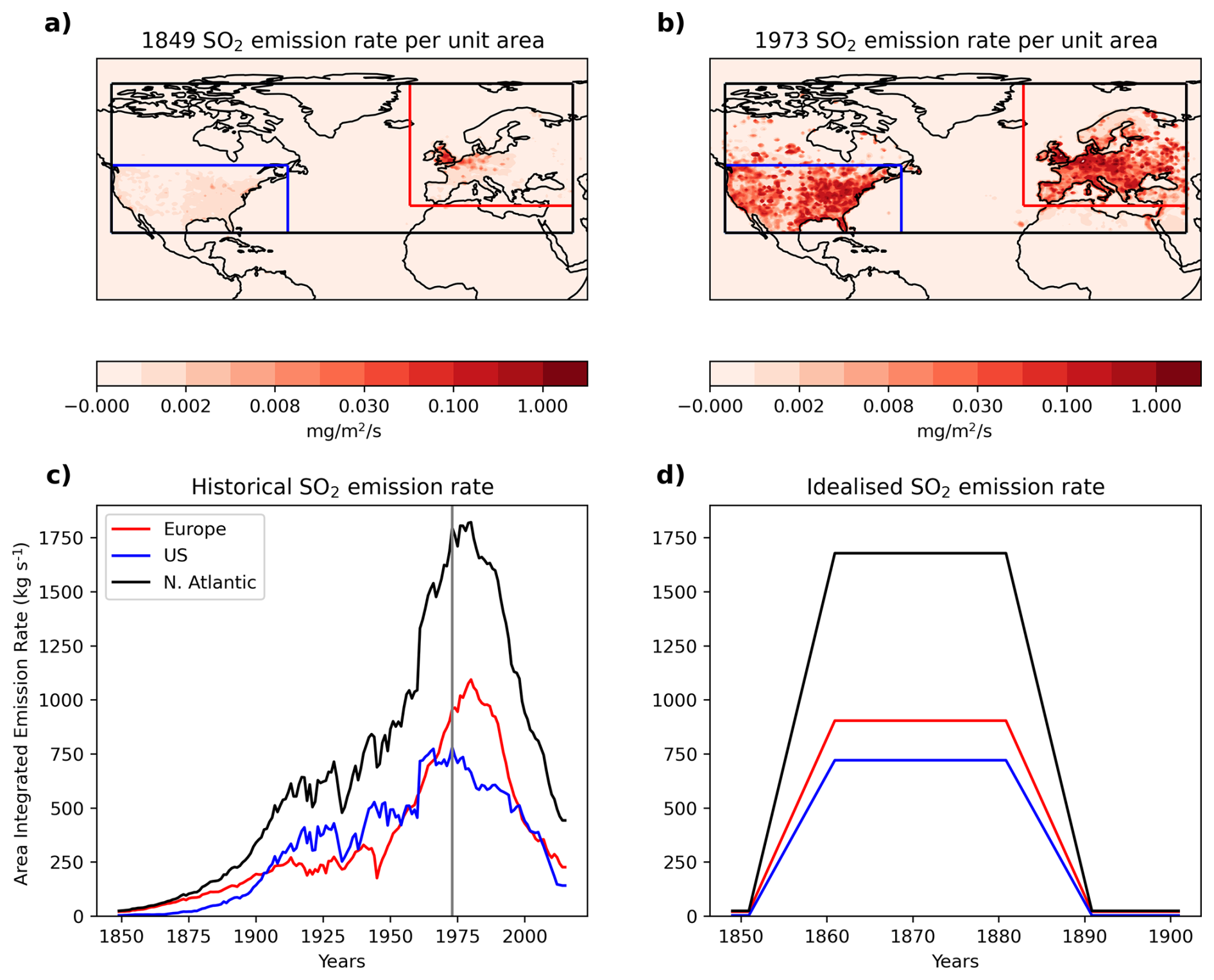
Figure 1 Spatial pattern and time profile of the applied idealised SO₂ emissions. Panel (a) shows the pattern of annual mean SO₂ emissions at year 1849, used as minimum emissions for the experiment. Panel (b) shows the pattern of annual mean SO₂ emissions in the year 1973, used as maximum emissions for the experiment. Note the non-linear colour bars. The black box indicates the North Atlantic sector. Only emissions within the black box are considered for the idealised experiment. The blue and red boxes bound the North American and European domains, respectively. Panel (c) shows the time series of regional mean historical SO₂ emission rates in the North Atlantic sector (black), North America (blue) and Europe (red). These three regions correspond to the regions marked in (a) and (b). Panel (d) shows the time series of the idealised SO₂ emission rates used in the experiments.

The reason for considering only SO₂ emissions (while omitting organic carbon, black carbon and dust) is because sulphate aerosol is the primary agent of AA radiative forcing during the historical period (Thornhill et al., 2021) and previous studies have found that multidecadal changes in SO₂ emissions have had the greatest influence on North Atlantic SST changes (Booth et al., 2012; Chang et al., 2011). The purpose of this set of experiments is to identify the specific mechanism linking these SO₂ emissions to the AMV, without the influence of competing sources of external forcing.

Asian SO₂ emissions are not considered, and only emissions from the North Atlantic sector are included in this experiment for the same reason; to simplify the situation and help isolate specific mechanisms. This is because the processes linking emissions from different regions to the North Atlantic are likely different. For example, North American and European aerosols do so predominantly through local short-wave changes (Booth et al., 2012; Chang et al., 2011), but Asian aerosols may affect the North Atlantic through complex teleconnection mechanisms such as Rossby wave train from the western North Pacific to Europe (Wilcox et al., 2019), with potentially competing effects. These atmospheric teleconnections could potentially lead to a weakening of the AMOC (Liu et al., 2024), but it is outside the scope of this study.

The timescale and magnitude of the idealised SO₂ emissions are chosen to simulate the multidecadal timescale of the historical SO₂ emissions. Timeseries of the historical SO₂ emissions across the North Atlantic sector are shown in Fig. 1c. The ramping-up and ramping-down of emissions in the idealised perturbation are designed to simulate the rapid rise and fall of emissions from the 1930s to the present day. Because the peak emissions of North America slightly lead the European emissions peak, a 15-year mean around 1973 captures the peak emissions of both regions and is therefore used as the maximum emission rate for the idealised perturbation. The idealised time series is useful for identifying key processes, because the projection of such a distinctive timeseries on different variables shows clear links between how different variables influence each other. In addition, seasonal cycles in the emissions are not considered in the single-forcing experiment; the emission ramp-up occurs at each monthly timestep of the model simulations.

This set of experiments is different to the Detection and Attribution Model Intercomparison Project (DAMIP, Gillett et al., 2016) and Precipitation Driver Response Model Intercomparison Project (PDRMIP, Myhre et al., 2017) experiments performed as part of CMIP6. The DAMIP experiment includes single-forcing simulations; however, global emissions are used, and the emissions follow the historical timeseries, making it more difficult to isolate specific mechanisms linking AA to North Atlantic SST changes. The PDRMIP experiment is more similar to our set of idealised experiments, including single-forcing simulations with additional regional emission simulations and idealised temporal evolution. However, the PDRMIP idealised temporal evolution is designed to test equilibrium responses instead of simulating historical changes, and the regional emissions are Europe-only or Asia-only.

1.1.3 Initialisation

A 4-member ensemble was run for 50 years for both MM and LL versions of the model. The initial conditions for each ensemble member are the same as the ones used for the CMIP6 historical simulations (Andrews et al., 2020). The initial conditions were chosen to minimise the chance of each ensemble member starting from a similar oceanic state by considering the two leading modes of multidecadal variability: the Interdecadal Pacific Oscillation (IPO) and the Atlantic Multidecadal Variability (AMV). The MM idealised experiments were initialised with initial conditions from 1850, 1885, 1930, and 1960 of the N216 PI-control and the LL experiments from 1850, 1885, 1930 and 1970 of the N96 PI-control. These initial conditions include positive and negative phases of both the IPO and AMV (Andrews et al., 2020). All anomalies in the following analysis are calculated by first taking the difference between each ensemble member and the time mean over their respective segment from the PI-control. This is to minimise the problem with drift in the PI control simulation. The ensemble mean anomalies are then calculated from taking a mean over the anomalies from each ensemble member.

1.2 TOA energy imbalance

The overall effect of the aerosol emission on spatial distributions of aerosol optical depth (AOD), total cloud fraction and its impact on the radiative effects at the top-of-atmosphere (TOA) and at the surface are shown in Fig. 2. Changes in AOD give an indication of the aerosol-radiation-interactions (ARI), and total cloud fraction shows how the spatial distribution of clouds change. A caveat here is that total cloud fraction only reflects one aspect of cloud changes and therefore does not reflect the full aerosol-cloud-interactions (ACI). For example, the Twomey effect (i.e. increased reflectivity of cloud, (Twomey, 1977) is not captured. However, the focus of this study is to understand the influence of aerosol on the climate rather than focus on individual aerosol processes. We then assess the total amount of aerosol-forced radiative changes by investigating the responses in the net top-of-atmosphere shortwave radiation (TOA SW) and net surface downward short wave radiation (DWSW). For both TOA SW and DWSW, positive (red) indicates downward anomalies and negative (blue) indicates upward anomalies in Fig. 2.

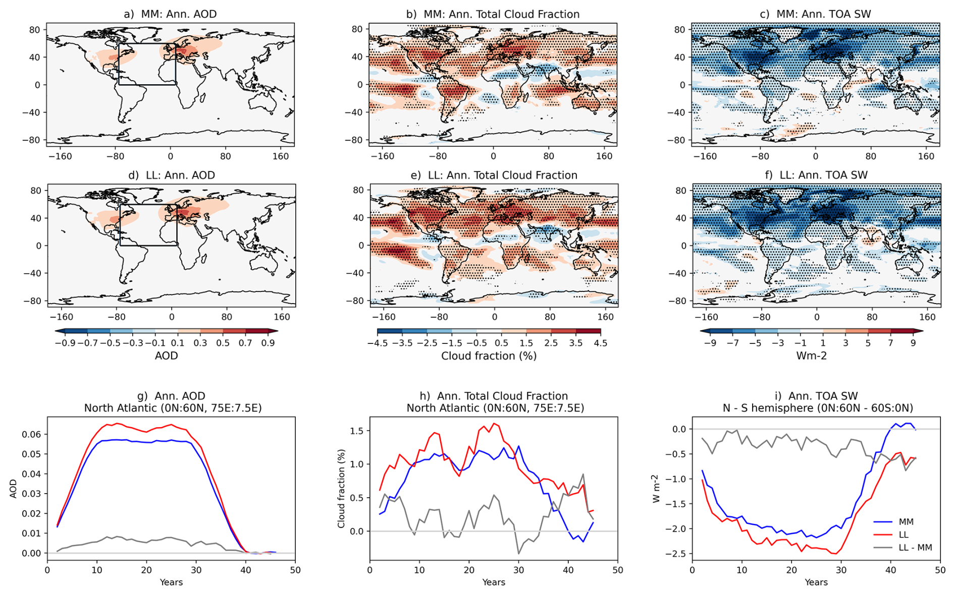
Figure 2 Spatial pattern and timeseries of the forced changes in aerosol optical depth (AOD), total cloud fraction and top-of-atmosphere net downward shortwave radiation (TOA SW). Panel (a) shows the spatial pattern of anomalous AOD averaged across years 10–30 of the forced simulation for MM. Panel (b) shows the same as (a) but for the total cloud fraction. Panel (c) shows the same as (a). but for TOA SW. Stippling indicates where the response is significant at the 10 % level, based on a two-tailed Student's t-test. Panels (d), (e), and (f) shows the same as (a), (b), and (c) but for LL. Panel (g) shows the timeseries of area-averaged annual-mean aerosol optical depth (AOD) taken across the North Atlantic basin (0 to 60° N, 7.5 to 75° E). Panel (h) shows the same as (g) but for the total cloud fraction instead of AOD. Panel (i) shows the interhemispheric difference (0 to 60° N minus 0 to 60° S) in downwards top-of-atmosphere net shortwave radiation (TOA SW) for MM (blue) and LL (red). The difference between the two models is shown in grey. All timeseries are smoothed by a 5-year running mean.

Figure 2a, d shows that the increase in SO₂ emissions results in an increase in AOD over the North Atlantic sector. Due to the short lifetime of tropospheric sulphate aerosols (3–7 d, Rasch et al., 2000), the largest AOD anomalies are located over the main emission regions; western Europe and the east coast of America. There are also weak AOD anomalies over the North Atlantic ocean and the Eurasian continent, which are downstream of the emission regions, indicating advection of aerosols.

The SO₂ emissions also induce an increase in total cloud fraction across much of the globe in both LL and MM (Fig. 2b, e). The largest increases in total cloud fraction are over the source regions. Outside of the source regions, there are also large and significant increases of total cloud fraction over the North Atlantic ocean and the Pacific ocean. There is a reduction of cloud fraction over India in both LL and MM, which is consistent with previous studies that show a weakening of the Indian monsoon in response to anthropogenic sulphate aerosol changes (Guo et al., 2016).

The timeseries in Fig. 2g, h, shows that the increase in AOD and total cloud fraction is consistent with the reduction in the total amount of solar radiation absorbed by the Earth, shown by negative anomalies in the TOA SW (Fig. 2c, f). Both models show strong negative TOA SW anomalies across the whole Northern Hemisphere, and weak anomalies across the Southern Hemisphere. The largest TOA SW anomalies are located over the aerosol source regions and the Arctic sea ice regions. Outside of these two regions over the Pacific and Atlantic oceans, negative TOA SW anomalies are co-located with increased total cloud fraction, indicating the importance of the cloud response in governing the overall energy imbalance.

A more quantitative comparison of the total aerosol forcing between the two models is shown by the time series in Fig. 2i. Since the aerosols are only emitted in the Northern Hemisphere, the interhemispheric difference of the total amount of absorbed solar radiation gives a measure of the strength of the aerosol forcing (Menary et al., 2020). This interhemispheric energy imbalance was found to correlate well with the magnitude of AMOC strengthening in CMIP6 historical simulations (Robson et al., 2022). Anomalies pole-wards of 60° N and 60° S are not considered to remove influences due to the sea ice response. The timeseries is smoothed by a 5-year running mean to minimise the year-to-year variability.

At both the surface and at the top of the atmosphere, the magnitude of the interhemispheric energy imbalance is greater in LL, by around 0.25 W m⁻² (Fig. 2i). This stronger forcing is related to both larger AOD perturbations and a stronger cloud response over the North Atlantic ocean (Fig. 2g, h). The specific aerosol processes at play are not the focus of this study.

2 Results

2.1 SST response

We begin the analysis by looking at the evolution of SST in response to the aerosol forcing before investigating the mechanisms which control these SST changes in later sections.

Figure 3 shows the evolution of the annual mean SST. The overall evolution of SST is similar between the two models. In both LL and MM, there is an initial (years 0–4) cooling across the North Atlantic. Northern Hemisphere SST continues to cool as SO₂ emissions reach their maximum (years 12–16). This cooling is especially large in the sea ice regions, in the Barents and Greenland-Iceland-Norwegian (GIN) Seas in both versions of the model and also the Labrador Sea (LS) in LL. However, the subpolar North Atlantic (SPNA) evolves differently from the rest of the basin. The SPNA becomes anomalously warm starting from years 16–20, and the warm anomalies continue to strengthen and persist to the end of the experiment. From years 38–42, the spatial pattern and magnitude of the SPNA warm anomalies are different between the two models. In MM, there are warm anomalies along the Gulf Stream extension region and in the central SPNA. In LL, the warm anomalies are weaker and lie only over the central SPNA. (Importantly, the interplay between the fast cooling and slow SPNA warming creates a disconnection between the SPNA and subtropical NA, which is not consistent with the observed AMV pattern, which instead shows a coherent, basin-wide variation in SST (Sutton et al., 2018). This indicates that in this model, the historical AMV is not mainly forced by changes in anthropogenic SO₂ emissions.)

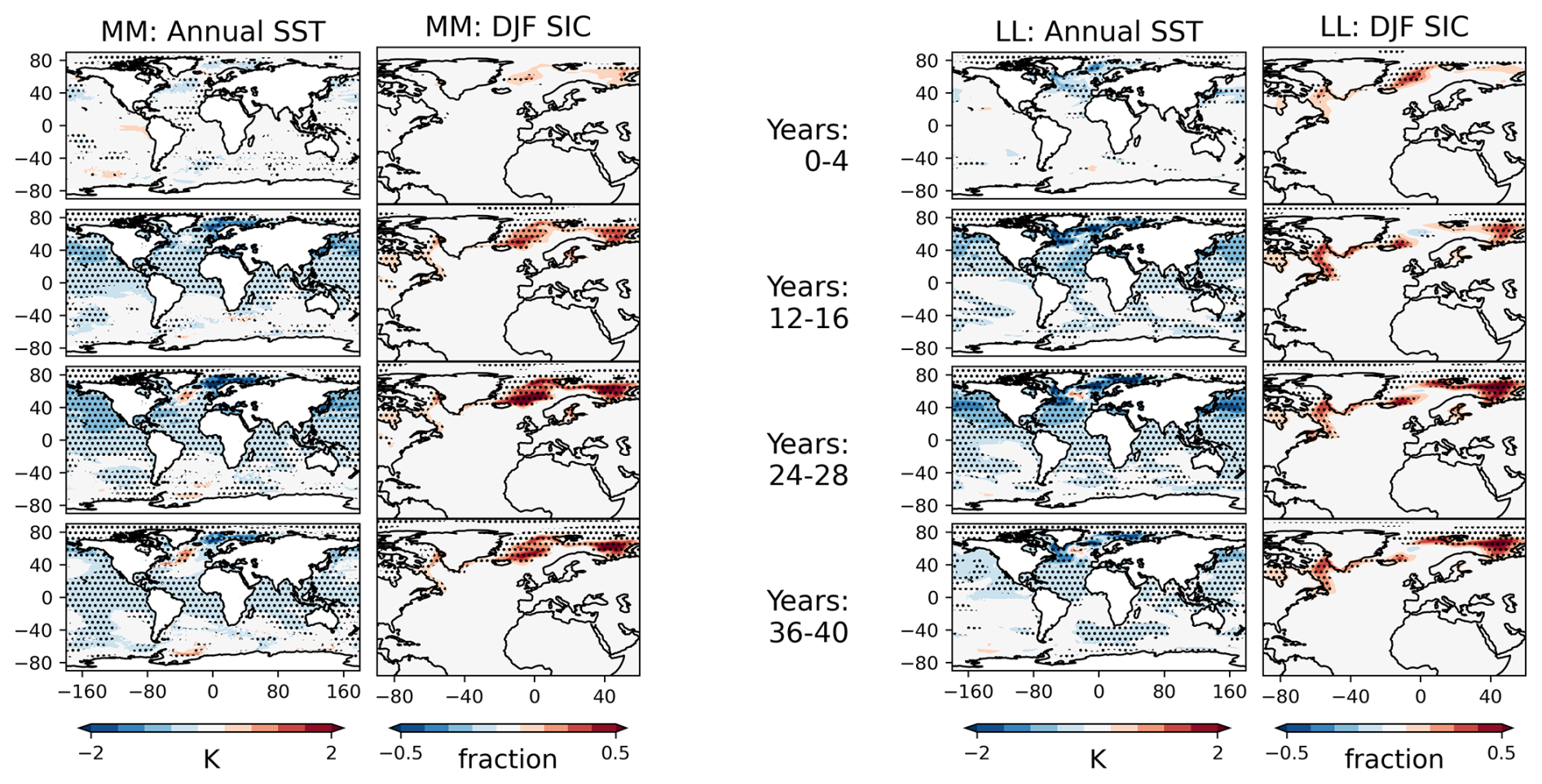
Figure 3 Spatial pattern and evolution of the annual-mean, ensemble-mean anomalies of sea surface temperature (SST) and winter (December–January–February, DJF) sea ice concentration (SIC). All variables are smoothed by a 5-year running mean such that Years: 0–4 represents the mean value between years 0 and 4. MM on the left and LL on the right. All variables are smoothed by a 5-year running mean. Stippling indicates where the response is significant at the 10 % level, based on a two-tailed Student's t-test.

The following subsections will explore in detail the mechanisms driving the SST changes. We will first examine the role of surface fluxes and the processes controlling these fluxes. We will then assess the role of forced ocean circulation changes. Specifically, we will look at the processes linking aerosol emissions to AMOC changes and how these differ between the two resolutions.

2.2 Role of surface heat fluxes

As mentioned in the introduction, there are two sets of proposed mechanisms linking aerosol forcing to SST changes in the literature, one is driven by surface heat fluxes (Booth et al., 2012), and the other by forced ocean circulation changes (Menary et al., 2020). Therefore, the following analysis will first focus on the role of surface heat fluxes and the relative importance of radiation versus turbulent heat fluxes (THF).

Section 1.2 has shown that there are indeed significant clouds and surface shortwave changes in both versions of the models; we now investigate whether aerosol radiative effects are the primary driver of surface temperature changes as proposed by Booth et al. (2012). We do this by decomposing the annual mean net surface heat flux (SHF) into contributions from turbulent heat fluxes (THF) and net downward shortwave radiation (DWSW). THF is defined as the sum of latent and sensible heat flux. Changes in the THF are driven by air-sea interactions and can be driven by changes in the atmospheric circulation (i.e. a stronger or weaker surface wind), or can be driven by changes in the air-sea temperature and humidity gradients. Changes in the net DWSW are linked to aerosol radiative effects including both aerosol-radiation interactions (ARI) and aerosol-cloud interactions (ACI). Changes in sea ice can also affect net DWSW through surface albedo changes. Although there are also other terms in the net SHF, such as net downward longwave radiation (DWLW), the sum of THF and net DWSW explained much of the total SHF. DWLW anomalies were the next largest term, but still an order of magnitude smaller than DWSW (not shown).

Figure 4 shows the evolution of total surface heat flux alongside the THF and net DWSW components. Positive anomalies (red) denote anomalous downward heat flux into the ocean, and negative anomalies (blue) denote anomalous upward heat flux out of the ocean and into the atmosphere. Both models show considerable spatial structure in the total surface heat flux. Initially, the total surface heat flux anomalies are small. As emissions increase, negative anomalies begin to develop across the subpolar North Atlantic (SPNA, 45 to 60° N). In contrast, positive anomalies develop across the Labrador, GIN and Barents Sea. This pattern of surface heat fluxes is reflected in the THF. Whereas, the net DWSW show a much more uniform cooling influence across the whole North Atlantic basin. This difference in spatial pattern indicates that it is air-sea interaction, rather than the aerosol radiative effect, which is the dominant control of the pattern of total surface heat fluxes averaged across the year. Furthermore, there are no significant changes in the sea level pressure (not shown), therefore, these AA forced THF anomalies are likely driven by temperature or humidity gradients (Robson et al., 2022) rather than surface wind changes (Hassan et al., 2021).

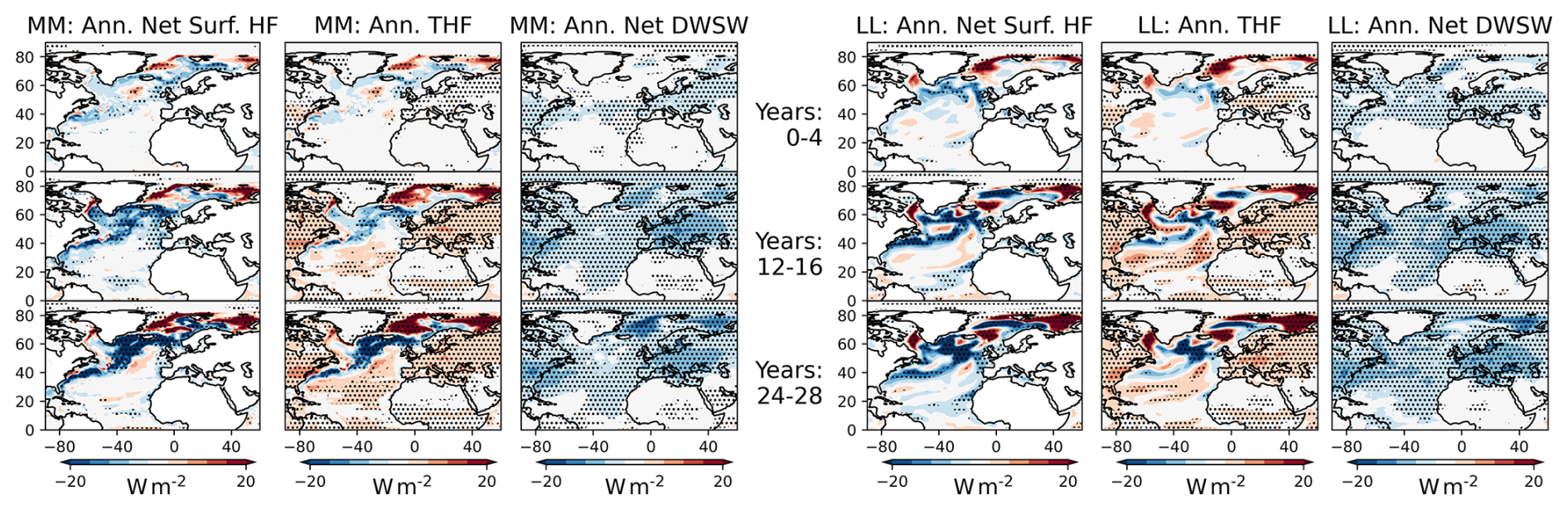
Figure 4 Spatial pattern and evolution of the annual-mean, ensemble-mean anomalies of net surface heat flux, turbulent heat flux (THF) and net downward shortwave radiation (DWSW). MM on the left and LL on the right. All variables are smoothed by a 5-year running mean. Stippling indicates where the response is significant at the 10 % level, based on a two-tailed Student's t-test.

Furthermore, the high latitude positive surface heat flux anomalies can be attributed to sea ice changes. Figure 3 shows the evolution of winter (December–January–February, DJF) sea ice concentration changes. In both LL and MM, the regions of largest sea ice growth are co-located with the positive surface heat flux anomalies (Fig. 4). This indicates that, averaged across the year, the dominant effect of sea ice on surface heat fluxes is through its insulating effect rather than its effect on surface albedo. Whereby, the growth of sea ice covers the ocean surface and inhibits air-sea interaction, resulting in less heat loss than usual. If the sea ice albedo effect were to dominate, then these high-latitude anomalies would be negative instead.

2.3 Ocean heat transport and AMOC changes

The previous section showed that different sections of the North Atlantic appear to respond differently to the aerosol forcing. In particular, surface fluxes on their own do not explain changes in the SPNA SST, i.e. the SPNA SST warms at the same time as strong anomalous surface cooling through THF. Therefore, in this subsection, we now look into the hypothesis that a forced AMOC response may be driving ocean heat content changes and SPNA surface warming. We first investigate the role of ocean heat transport before comparing the AMOC response between the different resolutions.

The evolution of ocean heat transport (OHT) is shown by the Hovmoller diagrams in Fig. 5. In both LL and MM, the northward OHT strengthens throughout the first 40 years, even as SO₂ emissions abruptly decrease after simulation year 30. There is positive OHT convergence between 35 and 60° N, consistent with the lagged SPNA SST response (Fig. 3). The OHT anomalies also exhibit strong latitudinal coherence in both LL and MM (i.e. anomalies appearing at all latitudes at once, with no clear lag between different latitudes). The magnitude of OHT anomalies is greater in MM compared to LL, which is consistent with the warmer SPNA SST anomalies in MM.

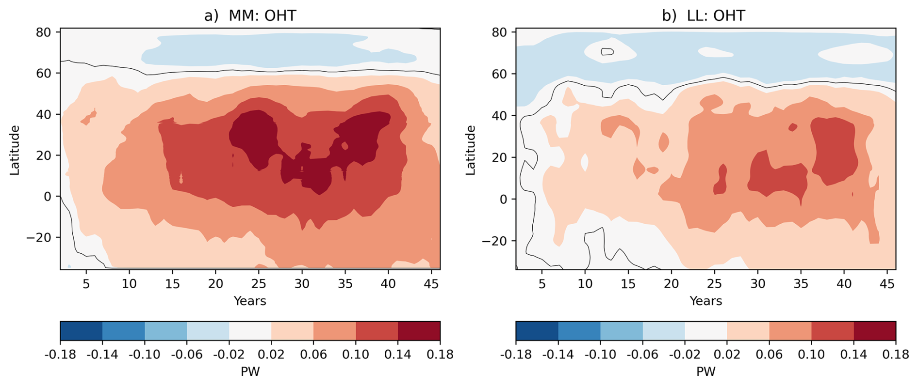
Figure 5 Hovemoller plot of northward OHT anomalies in the North Atlantic basin. Hovemoller diagrams of annual-mean, ensemble-mean anomalies of ocean heat transport (OHT) by latitude and time. Panel (a) shows the MM version of the model and (b) shows LL. All variables are smoothed by a 5-year running mean. All shaded regions are significant at the 10 % level based on a two-tailed Student's t-test. Stippling is left out for clarity.

The increase in OHT and convergence in the SPNA is consistent with a strengthening of the AMOC in response to the aerosol forcing. Figure 6 shows the evolution of the AMOC response in density space, with respect to a reference density of 0 dBar (AMOC-sigma) for the two models. The AMOC in depth space is included in Fig. A1 in Appendix A for completion. In contrast to depth space, AMOC-sigma does not show strengthening across all density classes in the subpolar latitudes (Fig. 6). Between 45 to 60° N, AMOC-sigma anomalies show a dipole pattern, negative anomalies in the lighter northward flowing waters and positive anomalies in the denser southward flowing waters. Furthermore, the largest positive anomalies are at the density class of 27.8 kg m⁻³, which is a denser class than where the maximum mean AMOC-sigma strength is in the PI control (27.6 kg m⁻³). This dipole pattern indicates that the AMOC does not uniformly strengthen across all density classes; instead, the AMOC appears to have shifted to a higher density class as it strengthens. This shift of density class as the AMOC strengthens has also been found in the CESM's (Community Earth System Model) preindustrial control simulation (Yeager et al., 2021).

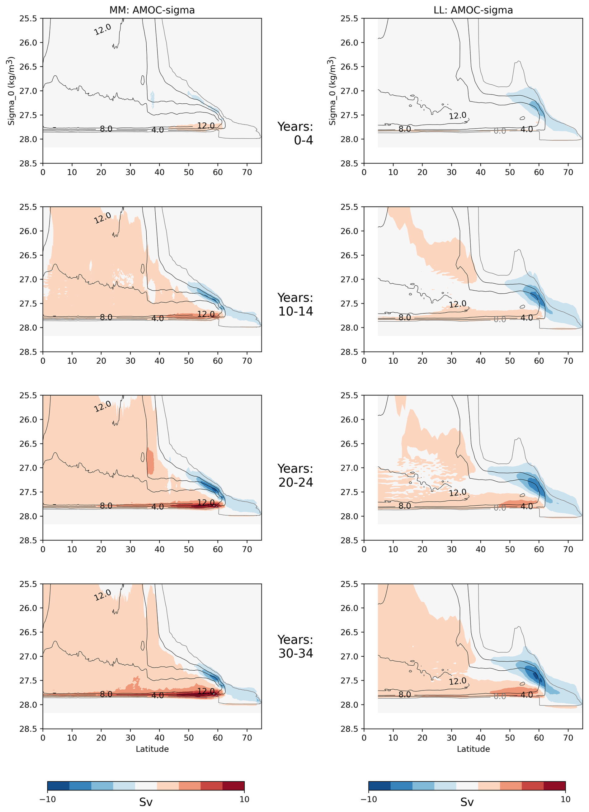
Figure 6 Evolution of the annual-mean, ensemble-mean anomalies of the AMOC streamfunction represented in density space (AMOC-sigma). The contour lines show the mean state of the pre-industrial control simulations, starting with 0 Sv represented by the grey line. Each subsequent contour has a spacing of 4 Sv. All variables are smoothed by a 5-year running mean. MM is shown on the left and LL is shown on the right. All shaded regions are significant at the 10 % level, based on a two-tailed Student's t-test. Stippling is left out for clarity to show both the mean state as contours and anomalies in shading.

The AMOC-sigma is a better representation of overturning at higher latitudes. Between 60 and 75° N, there is also a hint of overturning shifting to higher density classes in both LL and MM. However, these high-latitude positive anomalies are very weak and do not appear to be clearly connected to the stronger positive AMOC anomalies further south, suggesting that water mass transformation over the GIN Seas and transport of dense overflow waters are likely not a major driver of the wider AMOC strengthening.

In contrast to a previous study based on multi-model ensembles of CMIP6 historical simulations (Robson et al., 2022), the difference in the AMOC response is not correlated with the size of the aerosol-induced interhemispheric imbalance. In Robson et al. (2022), AMOC is highly correlated with the magnitude of energy imbalance (correlation coefficient of 0.8). However, in this set of idealised experiments, the medium resolution has a stronger AMOC response of ∼3 Sv compared to the lower resolution, despite a weaker interhemispheric energy imbalance of 0.25 W m⁻² (Fig. 1i). To explain the differences between the resolutions, we will investigate two different processes in the next subsections. First, we will look at the differences in local surface buoyancy forcing, then the potential role for slower feedback by looking at how the spatial pattern of density anomalies evolve.

2.4 Differences in surface buoyancy forcing

The water mass transformation framework can be used to understand how aerosol-forced surface fluxes lead to AMOC changes (Desbruyères et al., 2019; Groeskamp et al., 2019). This framework is based on an understanding of the AMOC as a system where volume transport is in thermodynamic balance with surface water mass transformation. In the absence of mixing, the diapycnal (i.e. across density level) volume flux associated with the AMOC above a certain density level and at a specific latitude is related to the amount of air-sea exchanges of buoyancy within regions where this particular density level (isopycnal) outcrops at the surface, and north of this specific latitude. In other words, the AMOC-sigma index (i.e. AMOC strength at a particular class of density), should be proportional to the magnitude of surface fluxes over where the key isopycnal outcrops to the surface. Therefore, this subsection will first define an AMOC-sigma index and then estimate the magnitude of surface dense water formation.

2.4.1 AMOC-sigma index

Figure 7a, b shows timeseries comparison of the standard AMOC in depth space (AMOC-z, defined at a depth of 1000 m, where the mean state is at maximum) against the AMOC in density space (AMOC-sigma, at density of 27.8 and 27.6 kg m⁻³), for the two different resolutions. Both the density and depth space timeseries are defined at 45° N. The two density levels are chosen to correspond with where the mean state and where the standard deviation is largest, respectively (Fig. 6). 45° N is chosen as the latitude to define the AMOC index, as it is the southern boundary of the western SPG and captures the water masses formed north of this latitude (Groeskamp et al., 2019) while minimising the influence of other model-dependent processes such as the southward propagation pathways of water masses (Ortega et al., 2021).

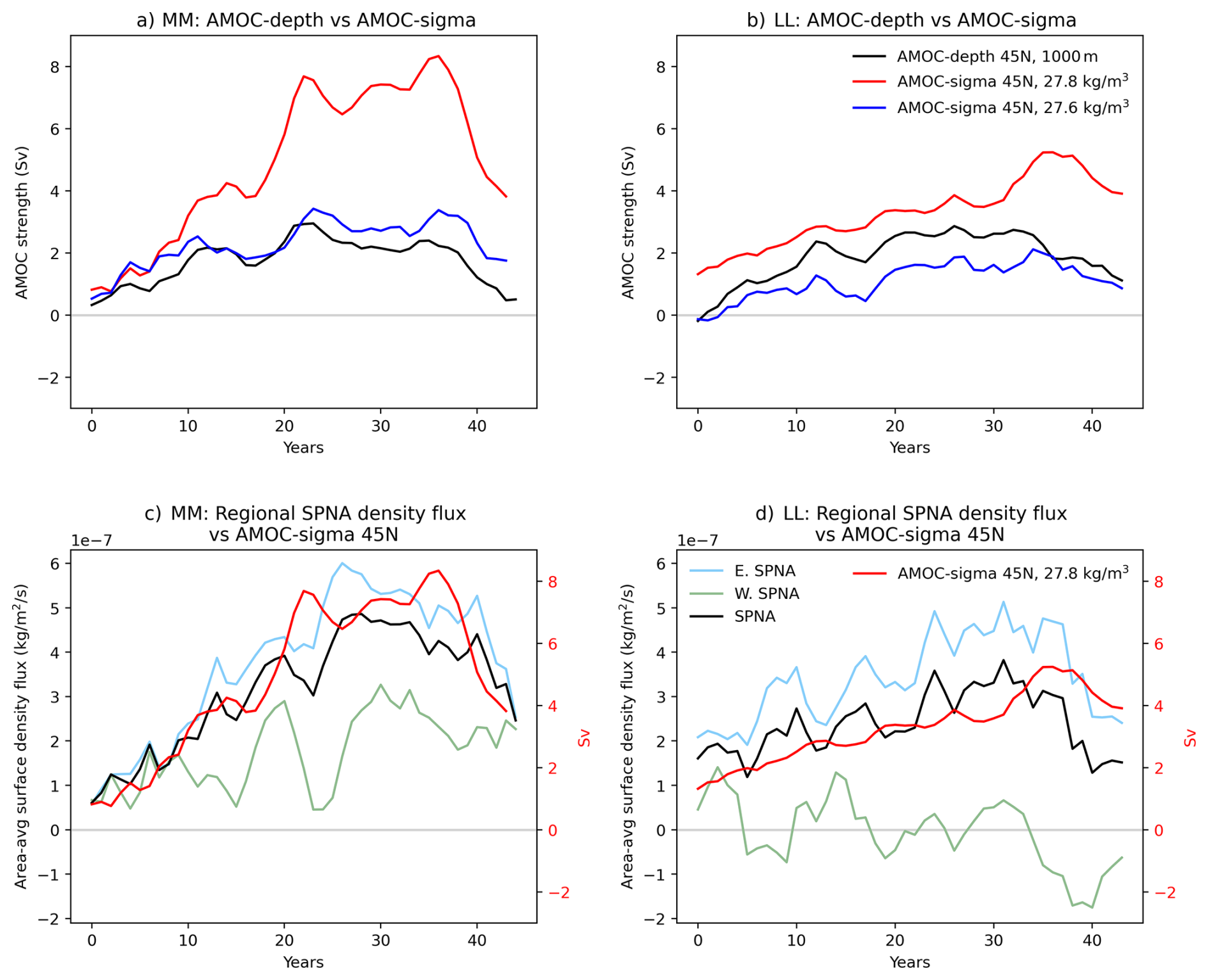
Figure 7 Panels (a) and (b) show the time series of the anomalous AMOC strength at 45° N, at depth of 1000 m (AMOC-depth 45° N, black), the timeseries of the maximum anomaly of the AMOC in density space at 45° N (AMOC-sigma 45° N) at density of 27.8 kg m⁻³ (red), and AMOC-sigma 45° N) at density of 27.6 kg m⁻³ (blue), for the MM and LL models respectively. Panels (c) and (d) show the time series of annual-mean anomalies of area-averaged surface density fluxes across the subpolar North Atlantic (SPNA, black) and contributions from the eastern (blue) and western (green) portion of the SPNA for the N216 and N96 models, respectively. The SPNA region is defined as (45–65° N, 65–0° W) and shown by black box in Fig. 9. The eastern and western portions are separated at Cape Farewell, shown by grey dashed line in Fig. 9. All variables are smoothed by a 5-year running mean.

The AMOC in depth space is not a good representation for this analysis because the same depth can contain waters of many different density classes due to the E–W density gradient at high latitudes. Indeed, the maximum AMOC-depth 45°N anomaly is 2.95 Sv in MM and 2.86 Sv in LL (Fig. 7a, b). There is also a larger difference between the AMOC-depth and AMOC-sigma index in MM, which is consistent with differences in the simulated AMOC structure related to model resolution. Higher resolution models tend to have a stronger E–W density gradient at high latitudes, therefore there is stronger cancellation between the light, northward flow and dense, return flow at the subpolar latitudes when represented in depth space (Hirschi et al., 2020). AMOC in density space tends to be a better representation for assessing the dynamics.

In density space, both indices at 27.8 and 27.6 kg m⁻³ capture a larger increase in MM (Fig. 7a, b). Although the magnitude of the AMOC-sigma anomalies and the inter-model differences are much more pronounced with the 27.8 kg m⁻³ index. The 27.8 kg m⁻³ index has a maximum anomaly of 7.89 Sv in MM and 5.24 Sv in LL, which is an increase of 52 % and 42 % over the maximum AMOC-sigma strength at 45° N in the PI control mean state for the MM and LL models, respectively. Whereas, the 27.6 kg m⁻³ index has maximum anomaly of 4.09 and 2.94 Sv in MM and LL respectively, corresponding to an increase of 30 % and 26 % from the maximum PI control mean. As shown in the previous section, the AMOC tends to shift to a higher density class as it strengthens, and we are interested in the difference in the AMOC response between the two resolutions, therefore we will use the AMOC strength at the denser level of 27.8 kg m⁻³ as the AMOC-sigma index hereafter.

2.4.2 Surface density flux

The combined effect of air-sea exchanges of heat and freshwater on sea water density (i.e. surface density flux) can be written as a function of the net surface heat (Q) and freshwater (F) fluxes as follows:

$$\begin{array}{}\text{(1)}& f=-{\displaystyle \frac{\mathit{\alpha }}{C_p}}Q-\mathit{\beta }{\displaystyle \frac{S}{\mathrm{1}-S}}F\end{array}$$

where α and β are the (positive) thermal expansion and haline contraction coefficients, C_p is the specific heat capacity of seawater, and S is the sea surface salinity (Speer and Tziperman, 1992). The sign convention used here is that positive (red in Fig. 8) denotes an increase in sea surface density and negative (blue in Fig. 8) denote a more buoyant sea surface.

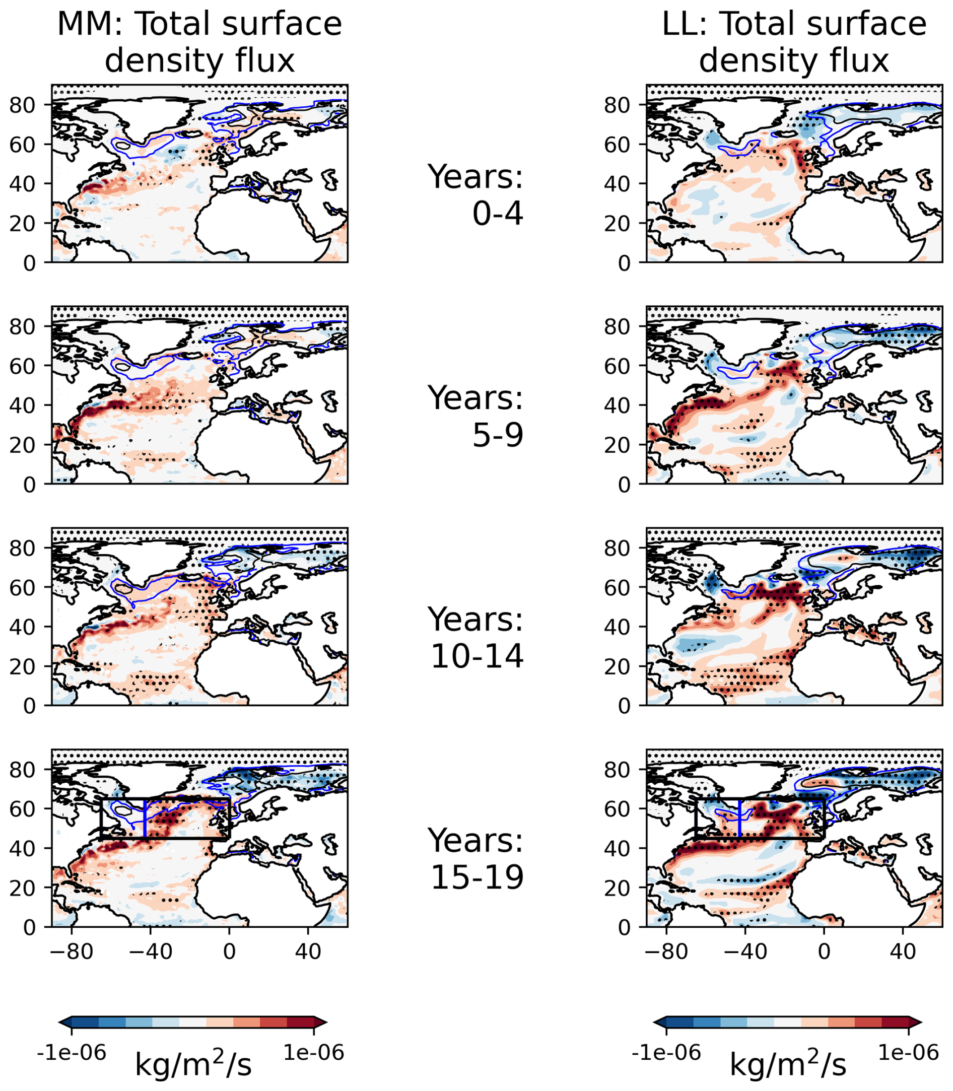
Figure 8 Spatial pattern and evolution of total surface density flux. Contours mark areas where key isopycnals outcrop to the surface in oceanic winter. The blue and black contour regions show where the isopycnals of 27.6 and 27.8 kg m⁻³, respectively, outcrop to the surface in the extended late-winter months (January–February–March–April, JFMA). All variables are smoothed by a 5-year running mean. MM is shown on the left, and LL is shown on the right. The black box in the bottom panels denotes the subpolar North Atlantic (SPNA) region defined as (45–65° N, 65–0° W). Stippling indicates where the response is significant at the 10 % level, based on a two-tailed Student's t-test

Figure 8 shows the evolution of annual mean surface density flux anomalies. Additionally, extended late winter (January–February–March–April, JFMA) ocean surface density 27.6 and 27.8 kg m⁻³ are highlighted by the blue and black contour lines as these density levels correspond to the maximum AMOC-sigma mean in the PI control and location of the largest AMOC-sigma anomalies in the idealised experiment respectively. The regions bounded by these contour lines indicate where these isopycnals outcrop to the surface, and therefore, the regions where surface forcing is directly driving the AMOC lower limb. The JFMA period is chosen because this is when the ocean surface is at its densest, therefore it is the period at which isopycnals of the densest water classes outcrop at the surface and water mass transformation occurs. Note that the surface density shown is the ensemble mean, not anomalies with respect to the PI control. This is because the absolute values of density are important for identifying specific density classes, not the relative changes. Figure 8 focuses only on the initial 19-years, to minimise the influence of the feedback from ocean circulation changes as the strengthening of AMOC and associated heat transport can also impact on the surface fluxes and water mass transformation.

In both LL and MM, two key regions are highlighted where the 27.6 kg m⁻³ density level consistently outcrops (i.e. blue contour lines, Fig. 8). These are the western SPNA (WSPNA) region and the Arctic region, which includes the GIN and Barents Seas. Note that the location and size of the two regions do not appear to change much with the varying levels of SO₂ emissions. The WSPNA outcropping region is larger in MM, spanning across much of both the LS and Irminger Seas (IS). Whereas, in LL, the WSPNA outcropping region is smaller and does not extend as far into the LS and IS. Additionally, the surface is denser in MM, with denser waters of 27.8 kg m⁻³ outcropping in the central LS, which does not occur in LL. In the Arctic, the regions of outcropping are more comparable between the two models (Fig. 8). The Arctic surface is very dense in both LL and MM, with the 27.8 kg m⁻³ level outcropping across the whole of the Barents Sea and much of the eastern GIN Seas.

Where key isopycnals outcrop in the WSPNA region, the surface density flux anomalies are generally positive in both LL and MM, which indicates that surface density fluxes here are responsible for driving the AMOC (Fig. 8). In the central SPNA, the large surface density flux anomalies are likely related to oceanic feedback, i.e. strengthening of the AMOC leads to a delayed warming of the SST, which then leads to more heat flux out of the ocean.

The relationship between surface density flux and the isopycnal outcropping region is different further north in the Barents and Kara Seas (Fig. 8). Although the surface of the Barents and Kara Seas is more dense than the SPNA with widespread outcropping of the 27.8 kg m⁻³ isopycnal, the surface density fluxes are generally negative. These negative surface flux anomalies are likely related to the growth of sea ice (Fig. 3), inhibiting heat flux into the atmosphere (Fig. 4), suggesting that deep water formation in the Barents and Kara Seas is likely not important for the aerosol-forced AMOC strengthening.

A further question here is the relative importance of surface heat versus surface freshwater fluxes in driving the overall surface density flux, as this can help narrow down the possible processes involved. The decomposition of surface density flux into its thermal and haline components, i.e. the two terms on the right-hand side of Eq. (1), is included in Fig. A2 in Appendix B. The thermal component dominates the total surface density fluxes throughout the whole simulation in both LL and MM. The haline component is an order of magnitude smaller than the thermal component. This result rules out many potential mechanisms involving freshwater fluxes, such as precipitation changes and sea-ice driven surface salinity changes, which have been proposed in previous studies, e.g. Menary et al. (2013).

Although we have shown that surface freshwater fluxes do not appear to play a big role in dense water formation, it does not mean that the salinity-controlled portion of density changes is unimportant for the overall AMOC response. The northward transport of salty water as the AMOC strengthens (Menary et al., 2013) or the southward transport of density anomalies in the Arctic (Jungclaus et al., 2005) may also play a role in changing the ocean density. The question of whether AMOC differences are related to differences in how density anomalies propagate around the North Atlantic basin will be explored in a later Sect. 2.5.

2.4.3 Surface-forced AMOC response and role of mean state differences

The previous section defined an appropriate AMOC-sigma index and showed that the SPNA is the key region of surface density flux. Figure 7c, d shows a comparison between the AMOC-sigma 45° N index and the timeseries of area-averaged SPNA surface density flux alongside its decomposition into contributions from the western portion (which includes the Labrador Sea only) and the eastern portion (includes the Irminger Sea and eastern SPNA), separated at Cape Farewell (regions shown by black box and dashed grey line in Fig. 9). Both models show a similar relationship between the AMOC-sigma strength and the total SPNA density flux (i.e. a similar amount of volume flux (Sv) per unit of density flux (kg m⁻² s⁻¹)). This agreement between the two models is consistent with previous studies showing that SPNA surface fluxes can strongly predict AMOC variability (Desbruyères et al., 2019). The stronger AMOC response in MM is also consistent with the larger density flux anomalies in the SPNA. In LL, the maximum density fluxes lag AMOC from year 30, which could be due to feedback from the AMOC strengthening, where increased northward heat transport also increases the SPNA SST and hence the surface heat loss and density fluxes.

The differences between the models are largely explained by differences in the western part of SPNA (Fig. 7c, d). The trend of surface density flux is positive in MM, but negative in LL. In contrast, the trend and magnitude of the eastern portion are more comparable between the two models. The higher maximum density flux in MM is likely related to an AMOC feedback, where the stronger AMOC response in MM results in stronger northward ocean heat flux and hence enhanced surface heat loss and stronger density flux.

What appears to explain the differences in both the size of isopycnal outcropping regions and the Labrador Sea surface density flux is the very regional difference in the sea ice response. Figure 9 shows the spatial pattern of the surface density flux plotted alongside the boreal winter (DJF) sea ice concentration with the 27.6 and 27.8 kg m⁻³ isopycnals overlaid as contours. Only the 5-year mean for years 24–28 is shown for brevity, the result described below holds true for any particular years. The overall pattern of surface density flux is largely similar in MM and LL except for the western and northermost side of the Labrador Sea. In MM, weakly positive surface density fluxes over the Labrador Sea are accompanied by minimal sea ice growth and widespread isopycnal outcropping of both the 27.6 and 27.8 kg m⁻³ density levels. In LL, surface density flux anomalies in the northernmost region of the Labrador Sea are strongly negative and are collocated with large positive anomalies in sea ice concentration. Sea ice growth will inhibit heat loss to the atmosphere, which results in reduced surface cooling and therefore negative density flux anomalies. Furthermore, the reduced surface density fluxes over this region also likely result in a more buoyant sea surface, which is consistent with the reduced area of isopycnal outcropping.

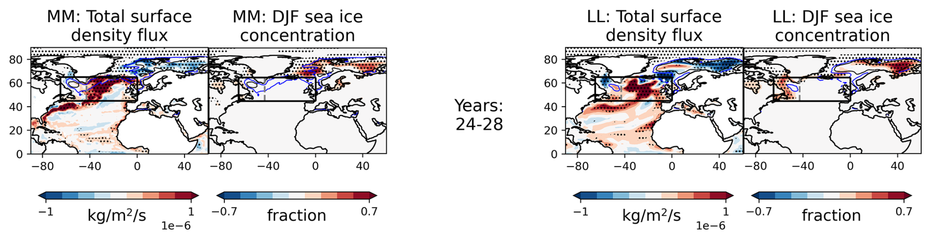
Figure 9 Spatial pattern of the annual-mean, ensemble-mean anomalies of surface density fluxes and December–January–February sea ice concentration (DJF SIC). All variables are smoothed by a 5-year running mean such that Years: 24–28 represents the mean value between years 24 and 28. MM is shown on the left, and LL is shown on the right. The blue and black contour lines represent the surface density levels of 27.6 and 27.8 kg m⁻³, respectively. The black box denotes the subpolar North Atlantic (SPNA) region. The eastern and western portions are separated at the cape of Greenland, shown by a grey dashed line. Stippling indicates where the response is significant at the 10 % level, based on a two-tailed Student's t-test.

The inter-model differences in sea ice response also appear to be consistent with differences in the model's mean states in the PI-control simulations. Figure 10 shows the mean state of winter sea ice concentration (DJF SIC) and annual mean SST in MM minus LL. In the mean state of MM, there is less LS sea ice but more sea ice in the GIN and Barents Seas. Where there is more sea ice in the mean state, there is also colder SST, which creates conditions conducive to sea ice growth. These mean state differences are consistent with the stronger LS sea ice growth in LL and stronger GIN and Barents Sea sea ice growth in MM. Although the sea ice differences in the GIN and Barents Seas are likely unimportant for the AMOC response to the aerosol forcing in these two models because anomalous surface density fluxes in the Arctic do not appear to play an important role for reasons discussed in Sect. 2.3.

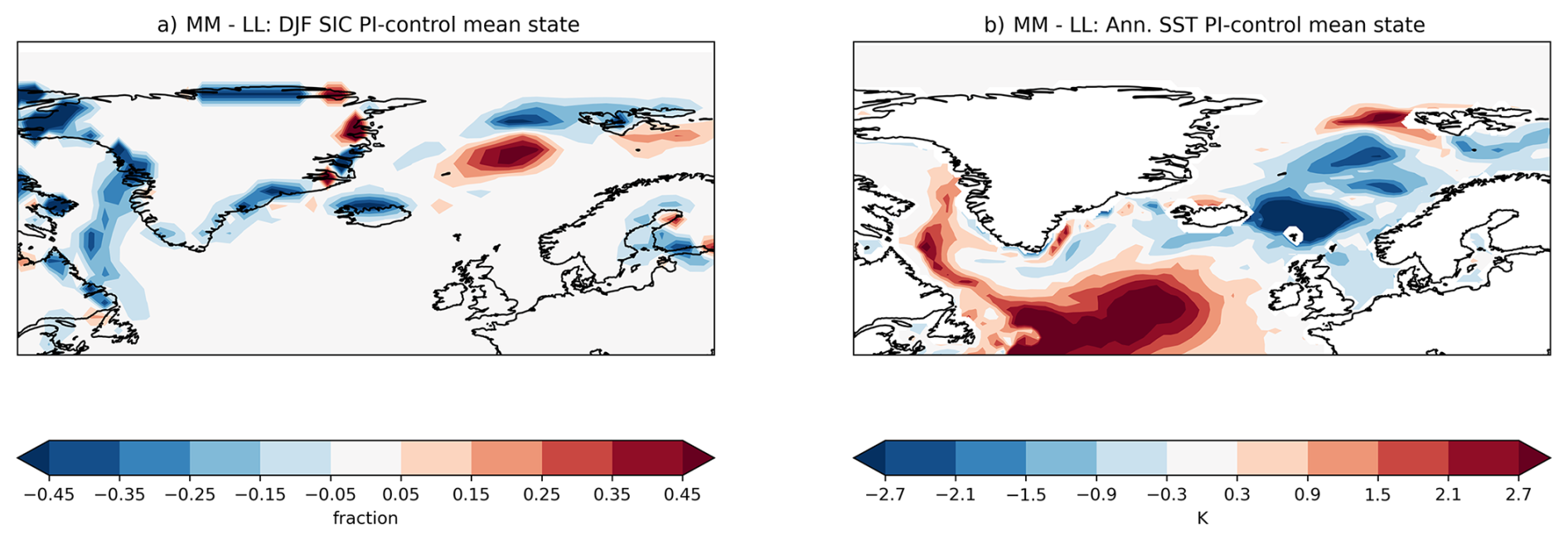
Figure 10 Panel (a) shows the inter-model difference (MM-LL) of the winter sea ice concentration (DJF SIC) mean state in the pre-industrial control simulations. Positive means more sea ice in MM, and blue means less sea ice in MM. Panel (b) shows the inter-model difference (MM-LL) of the annual mean SST mean state in the pre-industrial control simulations.

In summary, inter-model differences in LS sea ice response appears to control the magnitude and trend of SPNA surface density fluxes, and the size of isopycnal outcropping in the SPNA. The stronger sea ice growth in LL inhibits heat loss to the atmosphere and weakens surface density fluxes while also limiting the region of isopycnal outcropping. These two factors mean the total water mass transformation is weaker in LL, and likely explain why the AMOC response is weaker in the LL model despite a stronger overall aerosol-forced hemispheric energy imbalance. Furthermore, the differences in the sea ice response are consistent with the differences in the sea ice and SST mean states between the two models. Kuhlbrodt et al. (2018) showed that these mean state differences in SST and sea ice are related to the position of the Gulf Stream and North Atlantic Current, and the associated heat transport, which is more realistic in MM. A separate study found that these Labrador Sea biases also explain the disagreement between the observed and simulated overturning along the OSNAP (Overturning in the Subpolar North Atlantic Program) line in the HadGEM3-GC3.1 models (Petit et al., 2023).

2.5 Differences in propagation of density anomalies and role of salinity

Local surface heat forcing is not the only driver of AMOC strengthening. Transport of anomalously dense water driven by surface fluxes in remote regions or from ocean circulation feedback can also affect subpolar North Atlantic density and hence the AMOC (Menary et al., 2013; Vellinga and Wu, 2004; Cheng et al., 2018; Jungclaus et al., 2005). For example, Menary et al. (2013) showed that in the HadGEM2-ES model, the AMOC response to aerosol forcing is partly driven by the AMOC itself, where the strengthened AMOC contributes to the salinification of the SPNA by its increased northward transport of subtropical, salty water. Another possible mechanism involves the Arctic. Jungclaus et al. (2005) showed that changes in the East Greenland current and Denmark Strait overflow can influence the transport of density anomalies between the Arctic and North Atlantic. This leads to our final hypothesis: whether the difference in AMOC response is related to differences in how density anomalies propagate around the basin.

Figure 11 shows the evolution of upper-ocean (0–700 m) density anomalies alongside the relative importance of the thermal vs. the haline component. Figure 12 shows a similar diagnostic, but for the subsurface layer (1500–3000 m), which corresponds to the return branch of the AMOC. The intermediate layer (700–1500 m) is omitted as it mixes signal from the upper-ocean northward branch and the subsurface return branch of the AMOC. The thermal component of the ensemble mean density was calculated by using the same equation used for total density, but with time-varying ensemble mean temperature while holding the salinity at a climatological value corresponding to the first 160 years of the pre-industrial control. The full 500-year climatology was not used to avoid the influence of model drift, and the first 160 years cover the spread of all ensemble members' initial conditions. The haline component is calculated in a similar way to the thermal component, but with the temperature held at climatological value. The relative importance is then calculated by taking the difference between the magnitude of the thermal component minus the haline component (i.e. $\left|T\right|-\left|S\right|$), such that positive (green) denotes temperature is the dominant control on density anomalies and negative (pink) denotes salinity is the dominant control instead.

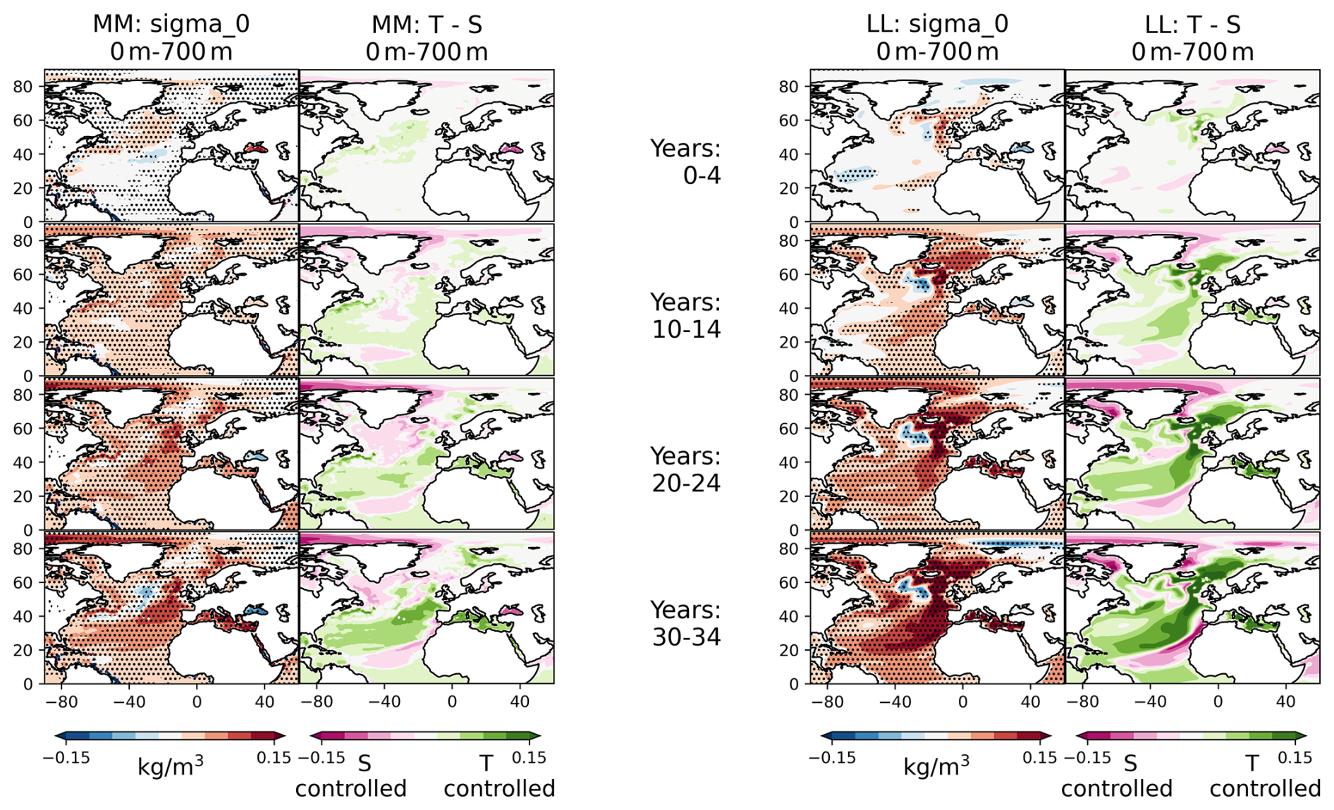
Figure 11 Spatial pattern and evolution of the annual-mean, ensemble-mean upper-ocean (0–700 m) potential density anomalies referenced to the ocean surface (sigma 0) alongside the relative importance of the thermal and haline components. Pink denotes that the density anomaly is dominated by the haline component, and green denotes a thermal dominance. MM is shown on the left, and LL is shown on the right. Stippling indicates where the response is significant at the 10 % level, based on a two-tailed Student's t-test.

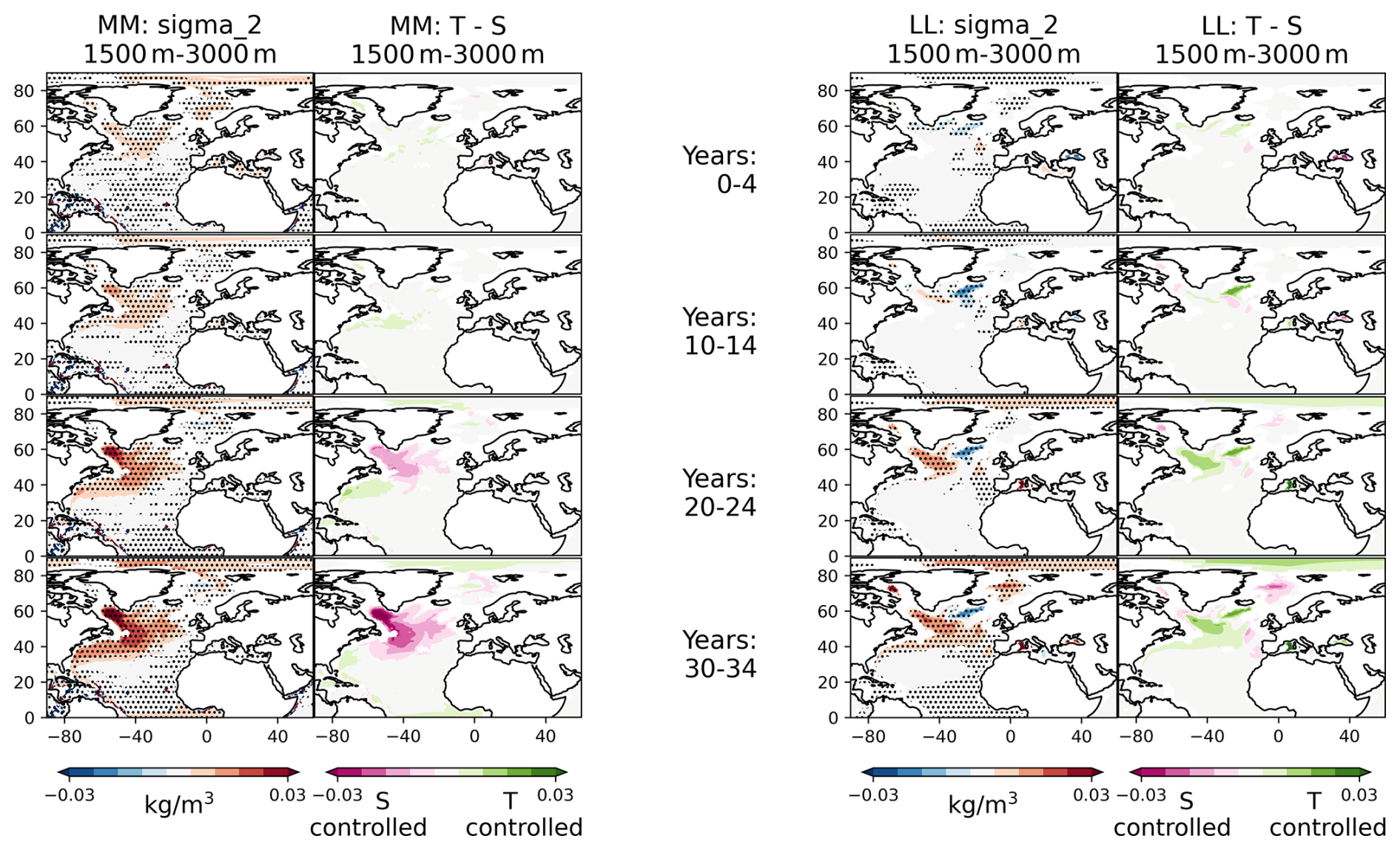
Figure 12 Spatial pattern and evolution of the annual-mean, ensemble-mean subsurface (1500–3000 m) potential density anomalies with respect to a reference pressure of 2000 dbar (sigma 2) alongside the relative importance of the thermal and haline components. Pink denotes that the density anomaly is dominated by the haline component, and green denotes a thermal dominance. MM is shown on the left, and LL is shown on the right. Stippling indicates where the response is significant at the 10 % level, based on a two-tailed Student's t-test.

In the upper ocean, both models begin with weakly positive density anomalies in the SPNA (Fig. 11). Very quickly, positive density anomalies become widespread across much of the basin, consistent with the hemisphere-wide cooling (Fig. 3). These positive anomalies strengthen until year 30–35, when SO₂ emissions are at their maximum. However, the central SPNA, the region just south of Iceland, evolves differently from the rest of the basin. In LL, negative anomalies appear as early as year 10–14 and strengthen until the end of the 50-year simulation. In MM, negative anomalies appear later, at year 20–24, but also strengthen until the end. The decomposition of these buoyant anomalies into thermal and haline contributions shows that this water mass is warm and salty (i.e., negative thermal contribution and positive haline contribution), which is a signature of the AMOC as it strengthens and transports warm salty water northward via the Gulf Stream and North Atlantic Current (Robson et al., 2016).

We now turn our attention to the western and central SPNA, which includes both the LS and IS. Both models show positive density anomalies, although with different relative contributions from temperature and salinity. In MM, both the thermal and haline components weakly contribute to the positive density anomalies in the first 14 years. From years 20–24 onwards, the haline component becomes the dominant component with the thermal component becoming a negative influence instead. In LL, this switch doesn't happen, the thermal component dominates across the SPNA, controlling both positive and negative density anomalies.

From 1500–3000 m, in both LL and MM, positive density anomalies appear first in the WSPNA region and propagate southwards along the deep western boundary (Fig. 12), which is a classic fingerprint of the AMOC (Buckley and Marshall, 2016). Similar to the upper-ocean, the relative importance of the thermal and haline components is different between the models. In MM, the density anomalies are initially driven by both the thermal and haline components. From years 20–24 onwards, the haline component becomes the dominant driver. On the other hand, in LL, the overall positive subsurface density anomalies in the western and central SPNA are largely dominated by the thermal component throughout much of the simulation. Positive haline anomalies do develop on the northern edge of the SPNA from years 30–34 onwards, but these are cancelled out by negative anomalies in the thermal component.

These results show an additional difference in the mechanism driving the AMOC response between the two models. In MM, although the initial density anomalies in both the upper and subsurface layers of the North Atlantic are temperature-dominated, the maintenance of high density anomalies increasingly becomes salinity-dominated with time. This indicates a key role in the salinification of the ocean in maintaining the strengthened AMOC. This change in the relative importance of temperature and salinity also indicates that the dominant driver of the AMOC response changes through time, with surface heat fluxes dominating first and then increased salinification maintains the strengthened AMOC. Furthermore, surface water fluxes are dominated by freshening due to increased ice melt, and so is not the cause of this salinification of the North Atlantic (Fig. A3 in Appendix C). Therefore, anomalous ocean-advection of salt is likely to be the key driver. This suggests a role for the slow salinity-advection feedback as proposed in Menary et al. (2013). In the lower resolution model, the salinification is weaker, which is consistent with the weaker AMOC response and hence weaker salinity-advection feedback. Note that this feedback is likely only active when the aerosol forced cooling is strong, which removes excess heat from the AMOC strengthening and allows salinity to control density anomalies. This switch from thermal to haline-controlled dense anomalies does not occur in the unforced pre-industrial simulations Lai et al. (2022). This switch also does not occur in observations (Robson et al., 2016), which is consistent with the fact that the aerosol forced cooling is much stronger in these simulations than in the real world.

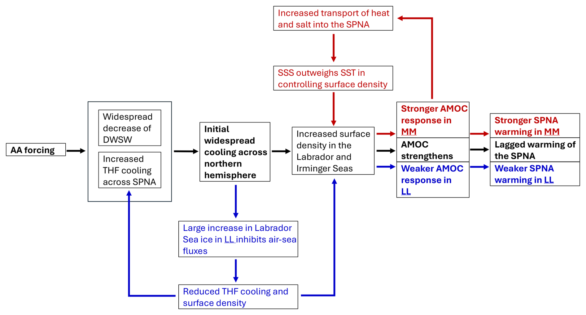
Figure 13 Schematic summarising the mechanism linking the idealised aerosol forcing to Atlantic SST and AMOC changes. Black arrows represent the processes common to both the medium (MM) and lower (LL) resolution models, i.e. the effect of aerosol forcing on surface heat fluxes, increased surface density and therefore, AMOC and SST. Red arrows represent the hypothesised salinity transport positive feedback, which is more evident in MM. Blue arrows represent the dampening influence of the LS sea ice response, which is stronger in LL.

3 Conclusions

Idealised single-forcing experiments were performed to investigate the effect of anthropogenic SO₂ emissions on North Atlantic climate variability. A time-varying source of North American and European SO₂ emissions, representing simplified historical emissions, was introduced to otherwise pre-industrial conditions. Two versions of the HadGEM3-GC3.1 model at medium (MM) resolution (≈ 60 km atmosphere, 0.25° ocean), and low (LL) resolution (≈ 130 km atmosphere, 1° ocean) were used to investigate the effect of model differences on the forced response. The key findings are summarised in the schematic Fig. 13 and as follows:

• The idealised aerosol forcing induces a fast, widespread SST cooling across the Northern Hemisphere and a slower warming in the subpolar North Atlantic (SPNA), which lags the rest of the Northern hemisphere by 15–20 years. The lagged SPNA warming is associated with a strengthening of the AMOC in both LL and MM, with a more pronounced AMOC response in MM compared to LL.

• MM has a stronger AMOC strengthening despite weaker aerosol-forced radiative changes, in contrast to previous studies (Menary et al., 2020; Robson et al., 2022). The difference in AMOC response is instead, consistent with stronger SPNA surface density fluxes (i.e. surface buoyancy forcing) and a denser sea surface (i.e. larger isopycnal outcropping area) in MM. These two factors indicate that there is likely stronger dense water formation in MM.

• Mean Labrador Sea SST and sea ice differences between LL and MM are a key factor in explaining the differences in the magnitude of AMOC response. LL has a climatologically cooler and more ice-covered Labrador Sea, leading to stronger sea ice growth as the aerosol cools the ocean surface. This leads to inhibition of air-sea fluxes and a reduction of isopycnal outcropping, which results in weaker dense water formation and weaker AMOC response.

• The difference in the AMOC response also appears to be related to how density anomalies propagate around the North Atlantic basin. In both LL and MM, positive surface density anomalies in the Labrador Sea change from temperature-controlled to salinity-controlled as the AMOC strengthens. This salinity-controlled surface dense water is therefore important for sustaining the strengthened AMOC and appears to be more important in MM. We hypothesise that there is a positive ocean-circulation feedback at play. The AMOC is initially forced by surface density fluxes, but the increased northward transport of salty subtropical water, coupled with the ongoing aerosol-forced surface cooling, maintains high density in the SPNA and sustains the strengthened AMOC basin. The stronger AMOC response and stronger salinity-dominated density anomalies in MM are consistent with a stronger positive salt-advection feedback.

The results from this study indicate that SST and sea ice biases in particularly sensitive regions such as the Labrador Sea can be important for the AMOC response and hence large-scale response to anthropogenic aerosol forcing. Mean state biases of the HadGEM3-GC3.1 model have been noted in the documentation paper, Kuhlbrodt et al. (2018), which attributes the difference in Labrador Sea SST and sea ice between the MM and LL models to the position of the Gulf Stream (GS) and North Atlantic Current (NAC). The GS and NAC are too-zonal in LL (typical of models at this resolution), resulting in more heat being transported into the GIN Seas and less heat circulating around to the Labrador Sea.

In contrast to many other modelling studies, which use multi-model ensembles to investigate model spread in AMV and AMOC mechanisms (Hassan et al., 2021; Menary et al., 2020; Wills et al., 2019; Ba et al., 2014), this study has instead focused on the same model at two different resolutions with minimal tuning differences. An advantage to this approach is that it allows for differences in relevant processes to be attributed to specific model differences and therefore provides additional insight, which would be otherwise missed in a multimodel ensemble. An example of this is in the difference in AMOC response to AA forcing. Results in this study stand in contrast to recent analysis on CMIP6 historical simulations (Robson et al., 2022; Menary et al., 2020); we find that the magnitude of AMOC response in this set of experiments is not correlated with the magnitude of the large-scale aerosol forcing, instead, regional differences in the mean state and resulting LS sea ice response appears to explain the difference in AMOC magnitude. This result indicates that looking at individual models may lead to a different interpretation on the cause of model spread. This conclusion has implications for the operational uses of climate models, where activities such as decadal prediction, detection and attribution, or climate risk assessment, might not utilise a large ensemble of models. This uncertainty highlights the need for a better understanding of the impact of individual model differences on the simulated physical processes, and the need for better observations in order to understand which sets of physical processes are more realistic and thus better constrain climate models. Furthermore, while this study focused on SO₂ emissions over the North Atlantic sector, which is the primary forcing agent in the historical period (Thornhill et al., 2021), emissions from other regions and other aerosol species can influence the regional radiation balance, cloud properties, and background circulations with potentially competing effects. Further experiments, perhaps following the RAMIP protocol (Wilcox et al., 2023), could be used to disentangle these mechanisms.

A disadvantage to this approach of analysing two very similar models is that we cannot be sure whether the inter-model differences identified are robust across other models, or if they are just unique to these two models themselves. For example, the differences identified could be just a result of mean state differences, which is not only a function of model resolution, and other models of similar resolution may have different mean state biases.

Nevertheless, there are good reasons to believe that higher resolution models may lead to better representation of the North Atlantic climate system. As climate models achieve increasingly higher resolutions, the representation of the dynamics becomes more realistic, since more processes are explicitly resolved and fewer processes have to be parameterised. More realistic representations of boundary currents and eddy transport can affect freshwater transport within the North Atlantic (Mecking et al., 2016). Higher resolution models tend to reduce surface temperature and salinity biases (Menary et al., 2015; Roberts et al., 2019), and they also tend to have stronger transport of heat and salt within the North Atlantic (Roberts et al., 2016, 2020). However, the long, millennial timescale required for ocean circulations to reach equilibrium may be prohibitively expensive to run on the highest resolution models. It must also be noted that greatly increasing horizontal resolution does not always guarantee improvements of model biases in all regions (Petit et al., 2023; Chassignet et al., 2020), and inclusion of mesoscale eddies may induce AMOC variability which is not yet observed in the real world (Hirschi et al., 2020). Therefore, progress in modelling techniques must be accompanied by progress in a process-based understanding of the effects of increasing resolution.

Appendix A

A1 AMOC in depth space

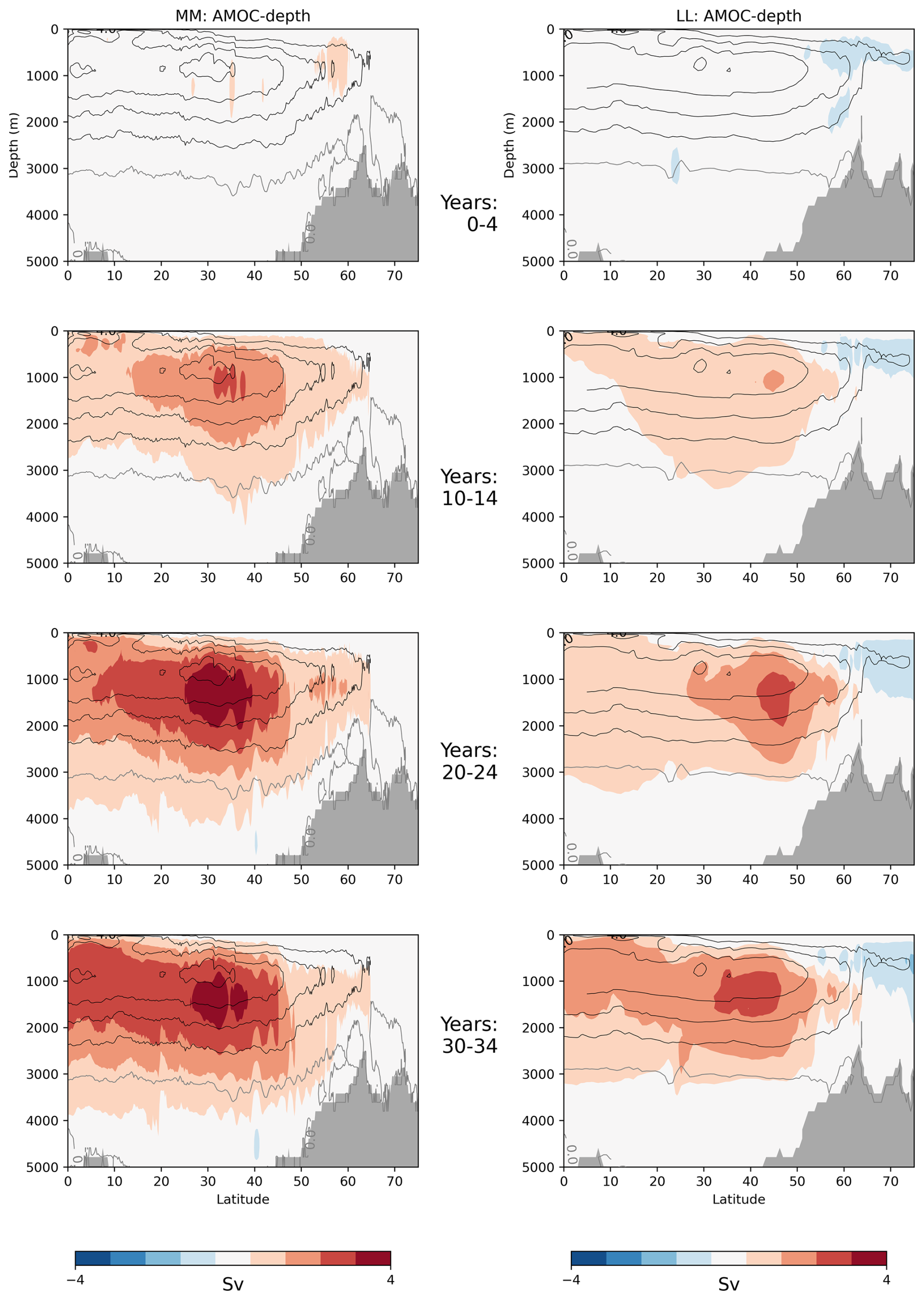
Figure A1 Evolution of the annual-mean, ensemble-mean anomalies of the AMOC streamfunction represented in depth space (AMOC depth). The contour lines show the mean state of the pre-industrial control simulations, starting with 0 Sv represented by the grey line. Each subsequent contour has a spacing of 4 Sv. All variables are smoothed by a 5-year running mean. MM is shown on the left, and LL is shown on the right. All shaded regions are significant at the 10 % level, based on a two-tailed Student's t-test. Stippling is left out for clarity to show both the mean state as contours and anomalies in shading.

A2 Thermal and haline components of surface density flux

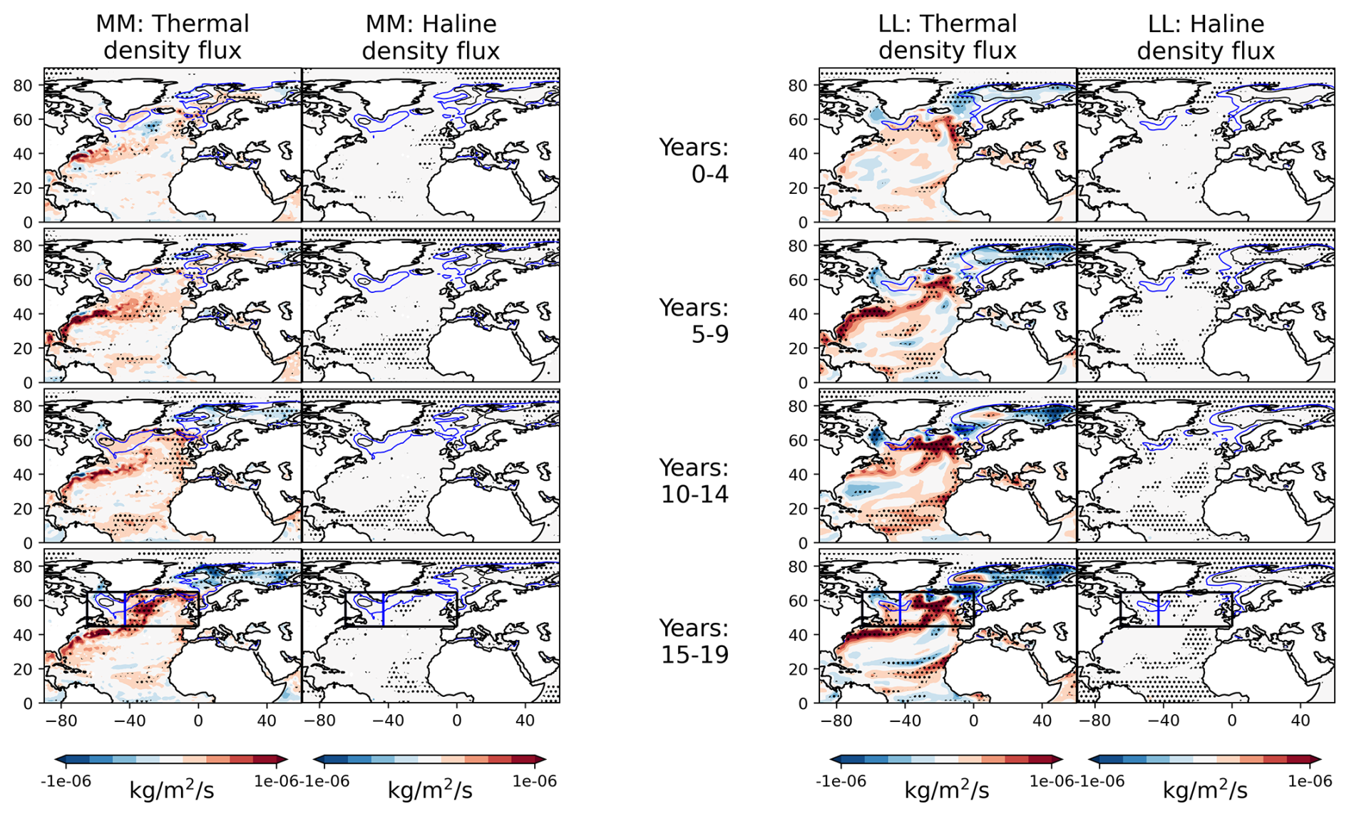
Figure A2 Spatial pattern and evolution of the decomposition of surface density flux into contributions from the haline and thermal components. Contours mark areas where key isopycnals outcrop to the surface in oceanic winter. The blue and black contours regions show where the isopycnals of 27.6 and 27.8 kg m⁻³, respectively, outcrop to the surface in the extended late-winter months (January–February–March–April). All variables are smoothed by a 5-year running mean. MM is shown on the left and LL is shown on the right. The black box in the bottom panels denotes the subpolar North Atlantic (SPNA) region defined as (45–65° N, 65–0° W). Stippling indicates where the response is significant at the 10 % level, based on a two-tailed Student's t-test

A3 Surface water flux components

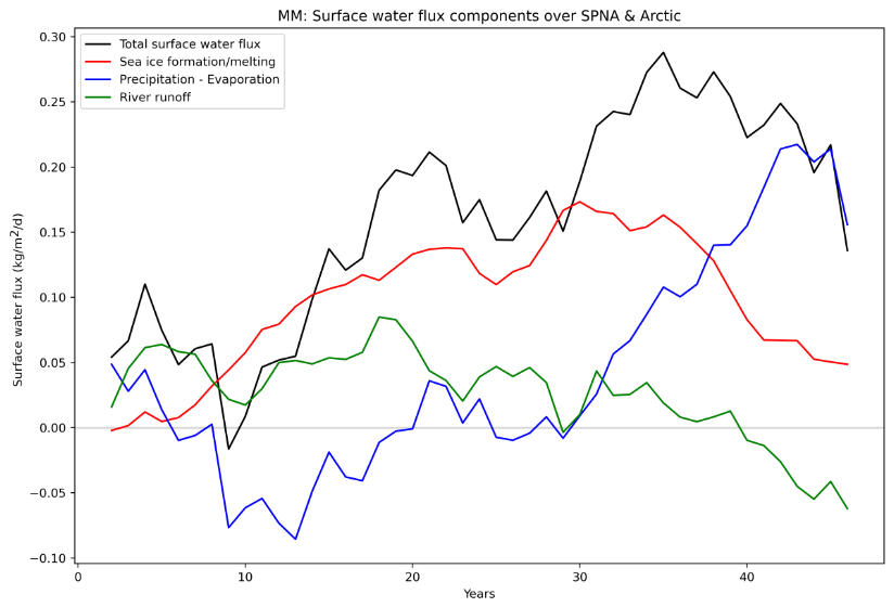
Figure A3 Time series of the anomalous total surface water flux (black) averaged across the Arctic and subpolar North Atlantic (45 to 65° N, 85° W to 35° E) alongside its decomposition; water flux due to sea ice melt/formation (red), precipitation minus evaporation (blue) and river runoff (green). Positive denotes anomalous surface water flux into the ocean. Only MM is shown. All variables are smoothed by a 5-year running mean.