Impact of black carbon on daytime valley and slope winds in idealised simulations

Thermally-driven valley circulation plays a key role in transporting air pollutants and heat in mountainous regions, yet the influence of absorbing aerosols on these local winds remains poorly understood. This study investigates how black carbon (BC) affects the daytime valley and slope winds using high-resolution idealised WRF-Chem simulations. The study consists of two simulations: one including realistic BC concentrations that interact with meteorological fields through absorption of incoming solar radiation, and a reference case without BC. When comparing the two simulations, absorption by BC leads to warming in the upper boundary layer and cooling in lower levels during daytime, enhancing boundary-layer stability and reducing surface heating. As a result, the up-slope winds that develop near the slope surface are weaker and flow in a shallower layer in the BC simulation. Although BC also weakens the pressure-gradient force between the plain and the valley that drives the up-valley winds, the up-valley winds in the afternoon become stronger than in the reference simulation. Momentum budget analysis for the valley volume shows that weaker up-slope winds reduce the export of momentum associated with up-valley winds out of the valley atmosphere, allowing stronger up-valley winds to form despite the weaker forcing. Overall, the results show that absorbing aerosols can modify the thermal structure in the valley and the exchange of heat and momentum between the valley atmosphere and surroundings, revealing a pathway through which aerosols can influence the valley and slope wind characteristics.

1 Introduction

Day-to-day air-quality in mountain regions is highly influenced by the thermally-driven valley circulation (Serafin et al., 2018). These local winds exhibit a diurnal cycle and develop due to topography induced horizontally heterogeneous heating in the lower troposphere. Under favorable conditions, such as fair-weather, weak large-scale forcing, and unstable or weakly stable stratification, the daytime valley circulation is efficient in transporting pollutants into the free troposphere and reducing pollutant concentrations in the near-surface layers (Serafin et al., 2018). However, the air-pollution can alter the incoming solar radiation and thus influence the heat distribution in the atmosphere (Su et al., 2020). In this article, we investigate how the absorption of incoming solar radiation by aerosols affects the thermally-driven valley circulation in idealised numerical model simulations.

Atmospheric aerosols alter the incoming solar radiation directly by absorption and scattering (Haywood and Shine, 1995), and indirectly by changing cloud properties (Rosenfeld et al., 2008). In this study we focus on the absorption. More specifically, our simulations include only one aerosol compound, black carbon (BC), which absorbs shortwave radiation strongly (Seinfeld and Pandis, 1998). BC is emitted directly into the atmosphere mainly from surface-based combustion processes (Briggs and Long, 2016) and has an important role in the anthropogenic aerosol particulate matter (Kirago et al., 2022; Zhang et al., 2025). Although BC is regionally transported, the highest concentrations are found near the emissions sources in the boundary layer (Bond et al., 2013). Despite its relatively short lifetime of a few days to weeks, BC can still reach remote locations such as high-altitude observatories, for example, in the Himalayas above 4 km altitude (Bonasoni et al., 2010; Xiang et al., 2021). The main removal pathways for BC are dry and wet deposition (Seinfeld and Pandis, 1998). Deposition of BC can change the snow and ice albedo and accelerate the cryosphere melting (Zhang et al., 2020; Kang et al., 2020). Deposition is included in this study but for simplicity, how the deposition of BC alters the surface properties, such as albedo, are not taken into account. Freshly emitted BC is very hydrophobic and ageing increases the hygroscopicity, typically within a timescale of one day (Bond et al., 2013). To exclude the changes in the BC aerosol population due to ageing during the simulation, in this study we include only aged BC and there is no further emissions or production by secondary processes of any aerosol compound during the simulations.

Absorbing aerosols, such as BC, heat the part of atmosphere in which they are located when subject to shortwave radiation. In the boundary layer (BL), the vertical distribution of the absorbing aerosols is crucial in defining how they affect the boundary layer structure and development (Ma et al., 2020; Slater et al., 2022). Within the convective BL aerosols are mixed typically up to the temperature inversion at the top of the BL. Above the inversion layer, in which the stable temperature profile inhibits vertical fluxes, the aerosol concentration decreases rapidly. Vertical heterogeneity in the aerosol distribution within the BL can stem, for example, from regional transport, growth of a surface-based stable inversion which decouples the surface layer from the rest of the BL (Slater et al., 2022), or local transport by thermally-driven valley circulation (Gohm et al., 2009). If absorbing aerosols are located near the BL top or right above it, the absorption of incoming solar radiation leads to warming and further increases the stability of the top of the BL. This reduces the shortwave radiation reaching the lower levels hence weakening the surface heating (Chen et al., 2022; Ma et al., 2020). Both of these effects reduce buoyancy in the BL and lead to reduced BL heights (Ding et al., 2016). This leads to a positive feedback, often referred to as the aerosol-boundary layer feedback (e.g., Petäjä et al., 2016; Su et al., 2020), in which the aerosol-radiation interaction reduces the BL height which further increases the aerosol concentration due to mixing into a smaller volume. The buoyancy suppressing effect of BC near the BL top or above it is referred as the dome effect (e.g., Ding et al., 2016; Wang et al., 2018; Ma et al., 2020). Through the dome effect, BC can prolong and intensify urban haze pollution episodes (Slater et al., 2022; Wang et al., 2023). However, the vertical profile of the absorbing aerosols is important (Ferrero et al., 2014; Ma et al., 2020; Slater et al., 2022). If more absorbing aerosol mass is located in the lower BL, the absorption heats the lower levels which promotes buoyancy and mixing in BL (Ma et al., 2020). The heating of the lower BL by absorption is referred to as the stove effect and it increases the BL height (Ma et al., 2020) and helps the dispersion of aerosols to reduce the near-surface concentrations (Slater et al., 2022).

The thermally-driven valley winds consist of along-valley winds and cross-valley winds. In the cross-valley direction, the winds flow up the slopes during the day and down the slopes during the night (Vergeiner and Dreiseitl, 1987). When the slope surface is heated by the incoming solar radiation, the air immediately next to the slope warms more than the air slightly away from the slope but at the same height. This leads to buoyancy acting along the slope and driving up-slope winds. The night-time down-slope winds form similarly when the air next to the cooling surface becomes denser than the air slightly away from the slope. The slope winds respond quickly to the changes in the surface thermal forcing and hence a shallow up-slope wind layer forms early in the morning shortly after the sunrise. Later in the day, when the whole valley atmosphere is neutral or unstable stratified, the up-slope winds still flow in a layer a few hundred meters deep, rather than rising vertically like typical convective plumes above flat ground (Vergeiner and Dreiseitl, 1987). The strength and depth of the up-slope winds depends on the surface heating, slope steepness, and the stability of the background atmosphere (Vergeiner and Dreiseitl, 1987; Farina and Zardi, 2023). The daytime cross-valley circulation includes also a return flow towards the valley centre above the up-slope wind layer and subsidence above the valley centre (Zardi and Whiteman, 2013). At the ridge-top height, the cross-valley circulation act on the exchange of heat, mass (e.g. air pollution), and momentum between the valley atmosphere and the troposphere above (Schmidli and Rotunno, 2012; Leukauf et al., 2015). In daytime, these fluxes include vertical outflow by the up-slope winds reaching the ridge-top and subsidence inflow into the valley volume from above the valley centre. In terms of heat exchange, the export of heat can reach up to 50 % of the energy provided by the surface sensible heat flux (Leukauf et al., 2015), depending on the thermal forcing. The mass transport can be notable as well – the mass export can reach up to five times the valley air mass during a day (Leukauf et al., 2016).

The diurnal cycle in the along-valley winds stems from the greater diurnal temperature oscillation in the valley atmosphere in comparison to the air above the adjacent plain (Serafin et al., 2018). The greater temperature oscillation is explained by a valley volume effect (Zardi and Whiteman, 2013), also referred to as the topographic amplification factor (TAF). The volume of air in the valley is smaller than the volume of air above the adjacent plain, when taking the same horizontal dimensions and depth of the valley. Given the same heat input at the top of the volume, the smaller air volume exhibits a greater heating rate. The warmer air in the valley during the day leads to a pressure-gradient force at low-levels directed from the plain towards the valley. This pressure-gradient force drives the plain-to-valley winds and therefore up-valley winds. Above the up-valley wind layer forms a return flow in the down-valley direction towards the plain. During the night the temperature difference between the plain and the valley volume is reversed and hence the low-level winds flow down the valley and from the valley into the plain. However, the difference in the air volume is a theoretical upper-limit for the excess heating of the valley volume, as the daytime cross-valley circulation exports heat out of the valley volume (Schmidli and Rotunno, 2010). Development of the up-valley winds is the result of heating the valley volume and hence their formation takes longer when compared to the up-slope winds (Vergeiner and Dreiseitl, 1987). The fully developed up-valley winds are found typically in the afternoon. The up-valley winds also flow in a deeper layer occupying even the whole valley volume cross-section and reach higher wind speeds than the up-slope wind. The factors which influence the occurrence, strength and depth of the thermally-driven valley circulation have been investigated in numerous studies by means of measurement campaigns (e.g. Whiteman and Doran, 1993; Weigel and Rotach, 2004; Rotach et al., 2016) and numerical modelling in both real (e.g. Weigel et al., 2006; Giovannini et al., 2017; Mikkola et al., 2023) and idealised (e.g. Wagner et al., 2015b; Schmidli and Rotunno, 2010) simulations. These factors include valley geometry, large-scale weather forcing such as cloud cover and atmospheric stability, surface properties such as soil moisture and snow cover, and thermal forcing at the valley surface.

The meteorological factors influencing pollution transport and pollution episodes in mountain regions are well reported in the literature. Pollution episodes in mountain valleys have been studied by means of observations and numerical simulations, emphasising, for example, the importance of the large-scale weather (e.g., Cordova et al., 2016), the formation of persistent temperature inversions in the valleys (Lareau et al., 2013; Largeron and Staquet, 2016; Quimbayo-Duarte et al., 2021), and the effect of surface properties such as snow cover (Chen et al., 2012; Whiteman et al., 2014). Transport processes in mountain regions have been studied by means of observations of air pollutants (e.g., Gohm et al., 2009; Chen et al., 2009; Duan et al., 2021) and numerical simulations including passive tracers (e.g., Wagner et al., 2015a; Lang et al., 2015; Quimbayo-Duarte et al., 2019; Rendón et al., 2020; Mikkola et al., 2025). A more complex approach, also using numerical simulations, is coupled meteorology-chemical transport modelling that has been applied to study the transport of specific aerosol compounds reaching the mountains (Zhang et al., 2020; Vitali et al., 2024; Bettineschi et al., 2025), the effect of complex topography on land-surface exchange processes (Reif et al., 2024), and the chemical transformation of aerosols along their transport (Li et al., 2011; Bei et al., 2018; Zhang et al., 2020; Ciarelli et al., 2025).

Despite the numerous studies on the meteorology controlling the air pollution in mountain regions, and on the factors that influence the valley circulation, the effect of aerosols on the thermally-driven valley winds is absent in the literature (to the authors' best knowledge). In this article, we investigate the impact of BC on the daytime thermally-driven valley and slope winds. This was done by performing two idealised simulations where one simulation has realistic BC concentrations which affect the thermodynamic and kinematic structure of the valley atmosphere through absorption of solar radiation, and one simulation with the aerosol-meteorology feedback switched off. We use the Weather Research and Forecasting model coupled with chemistry (WRF-Chem, Grell et al., 2005) which has shown good performance in previous studies focusing on the aerosol-boundary layer interaction with absorbing aerosols over flat terrain (e.g., Ding et al., 2016; Chen et al., 2022). The WRF-model (without the chemistry module, Skamarock et al., 2019) has been used successfully in idealised simulations focusing on the thermally-driven valley winds (e.g., Schmidli et al., 2011; Quimbayo-Duarte et al., 2019). Resolving the valley circulation accurately requires a high-resolution in the numerical model (Goger and Dipankar, 2024). Therefore our simulations incorporate a horizontal grid spacing of 200 m, which has been found suitable in previous studies with similar idealised setup (Wagner et al., 2015b). The article is structured as follows, the model setup and data analysis methods are described in Sect. 2, the two simulations are compared in Sect. 3 and the summary is given in the Sect. 4.

2 Methods

2.1 Model setup

We perform simulations using the Weather Research and Forecasting model coupled with chemistry (WRF-Chem) version 4.4.1 (Grell et al., 2005; Skamarock et al., 2019). WRF-Chem is coupled with a budget calculation tool WRFlux (Göbel et al., 2022) which provides flux computations and online time averaging. The use of WRFlux is further discussed in Sect. 2.2.

The model domain dimensions are 200 km in the y direction, 40 km in the x direction and the model top is at the height of 12 km. The horizontal grid spacing is 200 m and the simulations are run with a 2 s time step. Sensitivity of the model results and overall conclusions to the horizontal grid spacing was tested with an additional simulation run with a horizontal grid spacing of 100 m and a time step of 1 s (see Appendix A for more details). The 50% reduction in the horizontal grid spacing results in a negligible change in the valley-volume-averaged fields or the general flow structure. The domain has 100 model levels with the lowest model level at 15 m above the surface and the model level spacing is less than 100 m below the height of 3 km (Supplement Fig. S1a). The domain has a 5 km deep w-Rayleigh damping layer at the top. The lateral boundaries are symmetric in y direction (along-valley) and periodic in x direction (cross-valley). The lateral boundary conditions in WRF-model are described in Chapter 6 in Skamarock et al. (2019). The idealised valley topography shown in Fig. 1 is defined by Eq. (B1) given in Appendix B. The valley is south-north oriented, 100 km long, 20 km wide (ridge-top to ridge-top distance), 2 km deep (ridge-top height) and the cross-valley shape is defined by a cosine function. In the along-valley direction, the other half of the model domain (y<0 km) is flat (i.e. is a plain), also 100 km long, except the gradual rise of the ridges near the valley entrance (0 km$>y\ge -\mathrm{12}$ km).

The simulations are run in LES-mode (large-eddy simulation) with a three-dimensional 1.5-order TKE (turbulent kinetic energy) closure, third order Runge-Kutta time-integration, fifth order horizontal advection, and third order vertical advection of both momentum and scalars. No boundary layer scheme is used in the simulations. Surface layer physics are parameterised using Janjic Eta similarity scheme (Janjic, 1994). Land surface physics are parameterised using the unified Noah land surface model (Tewari et al., 2004) which has 4 soil layers. Microphysics are parameterised using the Purdue-Lin scheme (Chen and Sun, 2002), however no clouds are formed during the simulations. Shortwave and longwave radiation is parameterised using the RRTMG scheme (Iacono et al., 2008). Terrain features affecting the radiation (slope angle and topography shadowing) are considered (Zängl, 2002) and the radiation is updated every 60 s. The latitude of the domain is set at 28 degrees North, and the simulation is initialized for the equinox, when daylight is 12 h.

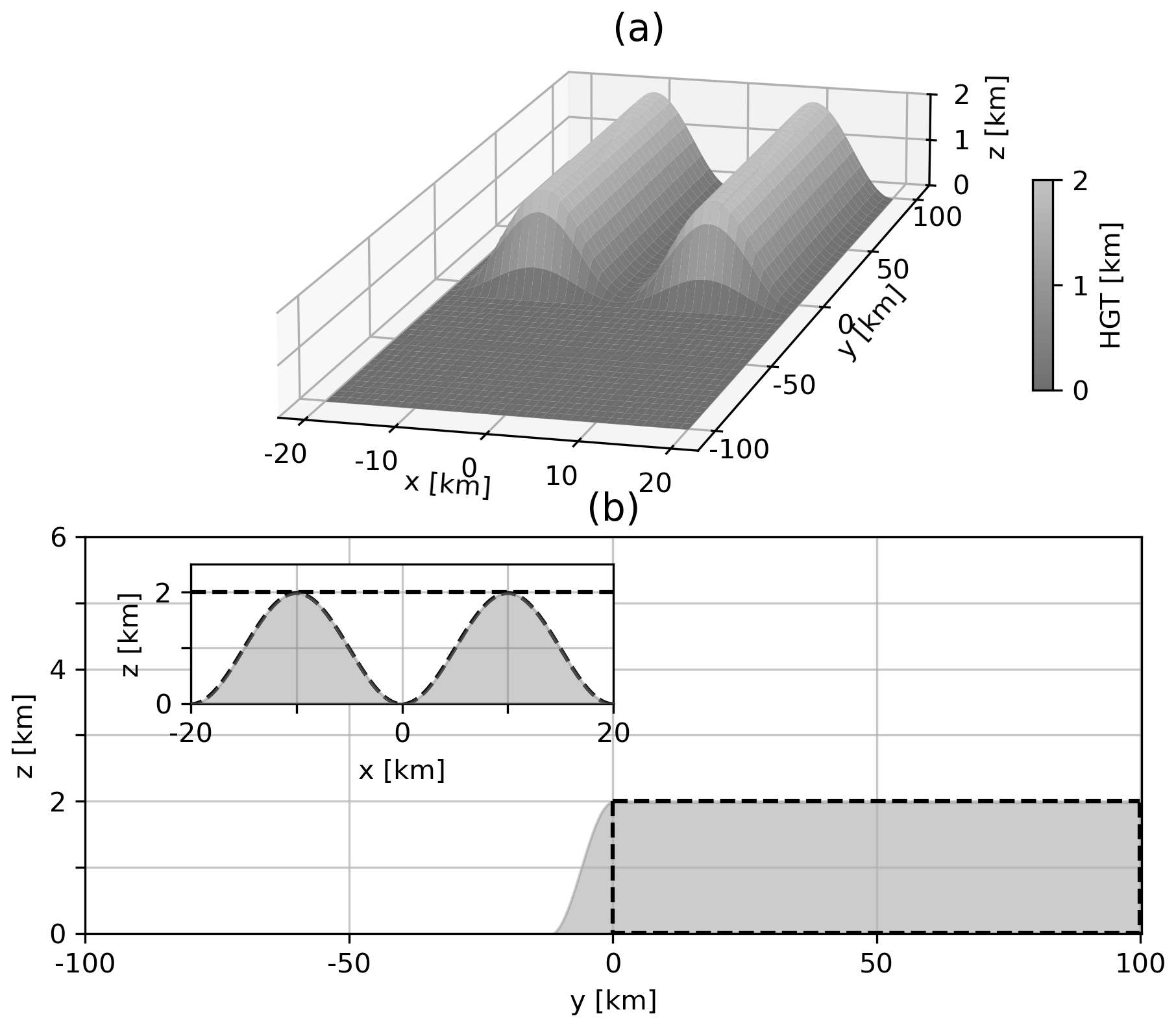
Figure 1 (a) Idealised valley topography. (b) Gray shading shows the valley topography along $x=\pm \mathrm{10}$ km in the main figure and across y≥0 in the inlet figure. Black dashed lines enclose the valley volume referred in the analysis.

Two simulations are performed, one with aerosol-meteorology feedback and one without. These simulations are referred to as AER and CTRL, respectively. Both simulations are 24 h long starting at 06:00 local time in the morning. Henceforth, all times are local time. The simulations start from the same meteorological state, which is the result of a 24 h spin-up run without the aerosol-meteorology feedback. Case CTRL continues from the spin-up without any changes. Case AER continues from the spin-up, but now with the aerosol-meteorology feedback being switched on. The chemistry setup of case AER is described in the following paragraphs. The spin-up simulation is initialised with a stable atmosphere using a temperature of 295 K and a pressure of 1000 hPa at the altitude of 0 m, a constant Brunt-Väisälä Frequency of 0.11 s⁻¹ (Fig. S1b). The initial wind components and relative humidity are set to zero throughout the domain. The land use category and vegetation type are defined as evergreen needle-leaf forest uniform across the whole domain. Soil moisture is initialised as 0.1 m³ m⁻³ in all 4 soil layers. This causes a minimal moisture flux, leading to a surface latent heat flux at maximum of 10 W m⁻² (Fig. S2c). The simulation is relatively dry on purpose to avoid cloud formation, and in fact the surface sensible heat flux is one or two order of magnitude stronger than the latent heat flux during the simulation (Fig. S2b–c).

The chemistry is described by the GOCART (Goddard Chemistry Aerosol Radiation and Transport) simple aerosol scheme (chem_opt=300 in WRF-Chem). As we focus on black carbon (BC), all the other species than hydrophilic BC are set to zero in the model initialisation. During the 24 h spin-up run, BC is transported by developing winds and 3 % of the initialised total BC mass is removed by dry deposition at the surface. During the subsequent 24 h of simulation AER, an additional 1.5 % is removed by deposition at the surface. Neither BC nor any other compound are emitted or produced by secondary processes during the simulation. The aerosol optical properties are computed using the exact shell approximation method, which assumes a shell surrounding the BC core and incorporates a full Mie calculation (Ackerman and Toon, 1981). The particle size distribution of BC in this aerosol scheme is 25 % of modal mass in Aitken mode and 75 % in accumulation mode. The aerosol processes (dry deposition and radiation) are updated every 60 s. As already said in the Sect. 1, we only include aged hydrophilic BC.

The 24 h-long spin-up run is initialised with an idealised BC profile with high concentrations near the surface which decrease rapidly with height (Fig. 2f). By initializing most of the BC mass near the surface, we ensure its transport and redistribution will primarily occur within the boundary layer during the simulation, reflecting its typical real-life location (Bond et al., 2013). Consequently, the actual AER simulation starts after a 24 h spin-up with a BC field that has been adjusted to a realistic boundary layer structure (Fig. 2b, g), rather than with the artificial idealised vertical shape of the initial state (Fig. 2a, f). The BC concentrations in AER are up to 17 µg m⁻³ in the boundary layer after the spin-up (Fig. 2g) and the BC column mass is around 2 mg m⁻² above the plain and the valley centre (not shown). For reference, Putero et al. (2018) reported a daily average of 10.2 µg m⁻³ of surface BC concentration during 2013–2015 in Kathmandu, Nepal, located in the Himalayan foothills. Wiedensohler et al. (2018) reported daytime surface BC concentrations between 8 to 20 µg m⁻³ during September and November 2012 in La-Paz, Bolivia, located in the Andes. Ferrero et al. (2014) reported mean BC concentrations of 8–10 µg m⁻³ throughout the mixed layer during February 2010 in Milan, Italy, located in the Po valley. In Beijing, China, the surface BC concentrations reach 20 µg m⁻³ and beyond during haze pollution events (Ding et al., 2016; Wang et al., 2018). Wang et al. (2013) estimated the BC column mass in Beijing using ground-based remote sensing and reported an annual variation between 2.7 and 7.3 mg m⁻² in 2009–2010.

2.2 Data analysis

Budget computation and online time-averaging is handled by the WRFlux-tool (Göbel et al., 2022) v1.4.1 which is a fork of the default WRF v4.4.1 repository (Göbel, 2022). All the model output shown in this article is based on the hourly averages from WRFlux. The analysis focuses on the valley volume, which refers to the air volume defined by y≥0 km and z≤2 km, shown by the dashed lines in Fig. 1b. As the lateral boundaries of the model domain are periodic in the x-direction, an identical parallel valley is located across the model x-boundaries ($\left|x\right|>\mathrm{10}$ km) in addition to the valley in the middle of the domain ($\left|x\right|\le \mathrm{10}\mathrm{km}$). The analysis covers the whole domain width in the x-direction, meaning also the two valley halves at $\left|x\right|>\mathrm{10}$ km are included in the spatially averaged or integrated values.

Along-valley momentum and heat budgets are retrieved using the post-processing tool of WRFlux to compute the tendency of each budget term from the hourly averaged WRFlux output. The tendency budget terms include transport of heat and momentum decomposed into resolved mean advection (referred to as ADV in this study), resolved turbulent (TRB) and sub-grid-scale (SGS) diffusion components using Reynolds decomposition (Göbel et al., 2022). The momentum budget includes a tendency from the pressure gradient forcing (PGF) which is retrieved from the Runge-Kutta and acoustic step modules in WRF-Chem. The heat budget includes tendencies from the radiation scheme separately for shortwave (RSW) and longwave (RLW) components. The components ADV, TRB, and SGS are output in the x, y and z-directions. In this study, the y-component of the resolved transport and SGS diffusion is referred to as the along-valley component. The sum of the x and z-components is referred to as the cross-valley component. The along-valley momentum tendency is given as

$$\begin{array}{}\text{(1)}& {\displaystyle \frac{\partial v}{\partial t}}=\sum _i{F}_{v,i}={\mathrm{ADV}}_v+{\mathrm{TRB}}_v+{\mathrm{SGS}}_v+{\mathrm{PGF}}_v\end{array}$$

where v is the y-component of the wind vector. The heat tendency is given as

$$\begin{array}{}\text{(2)}& {\displaystyle \frac{\partial \mathit{\theta }}{\partial t}}=\sum _i{F}_{\mathit{\theta },i}={\mathrm{ADV}}_{\mathit{\theta }}+{\mathrm{TRB}}_{\mathit{\theta }}+{\mathrm{SGS}}_{\mathit{\theta }}+{\mathrm{RSW}}_{\mathit{\theta }}+{\mathrm{RLW}}_{\mathit{\theta }}\end{array}$$

where θ is the potential temperature. F_θ,i and F_v,i are the individual terms on the right-hand-side of the heat and along-valley momentum budgets, respectively. Finally, the post-processed tendency terms are mass-weighted over the valley volume to give the along-valley momentum and heat budget by

$$\begin{array}{}\text{(3)}& {\displaystyle \frac{\mathrm{1}}{M}}\underset{V}{\int }\mathit{\rho }{\displaystyle \frac{\partial S}{\partial t}}\mathrm{d}V=\sum _i{\displaystyle \frac{\mathrm{1}}{M}}\underset{V}{\int }\mathit{\rho }{F}_{S,i}\mathrm{d}V,\end{array}$$

where S is either v or θ, M is the total mass of air in the valley volume V and ρ is the dry air density. The volume integral of Eq. (3) is approximated by a mass-weighted sum of the contribution of all grid boxes in the valley, taking into account the grid box volume.

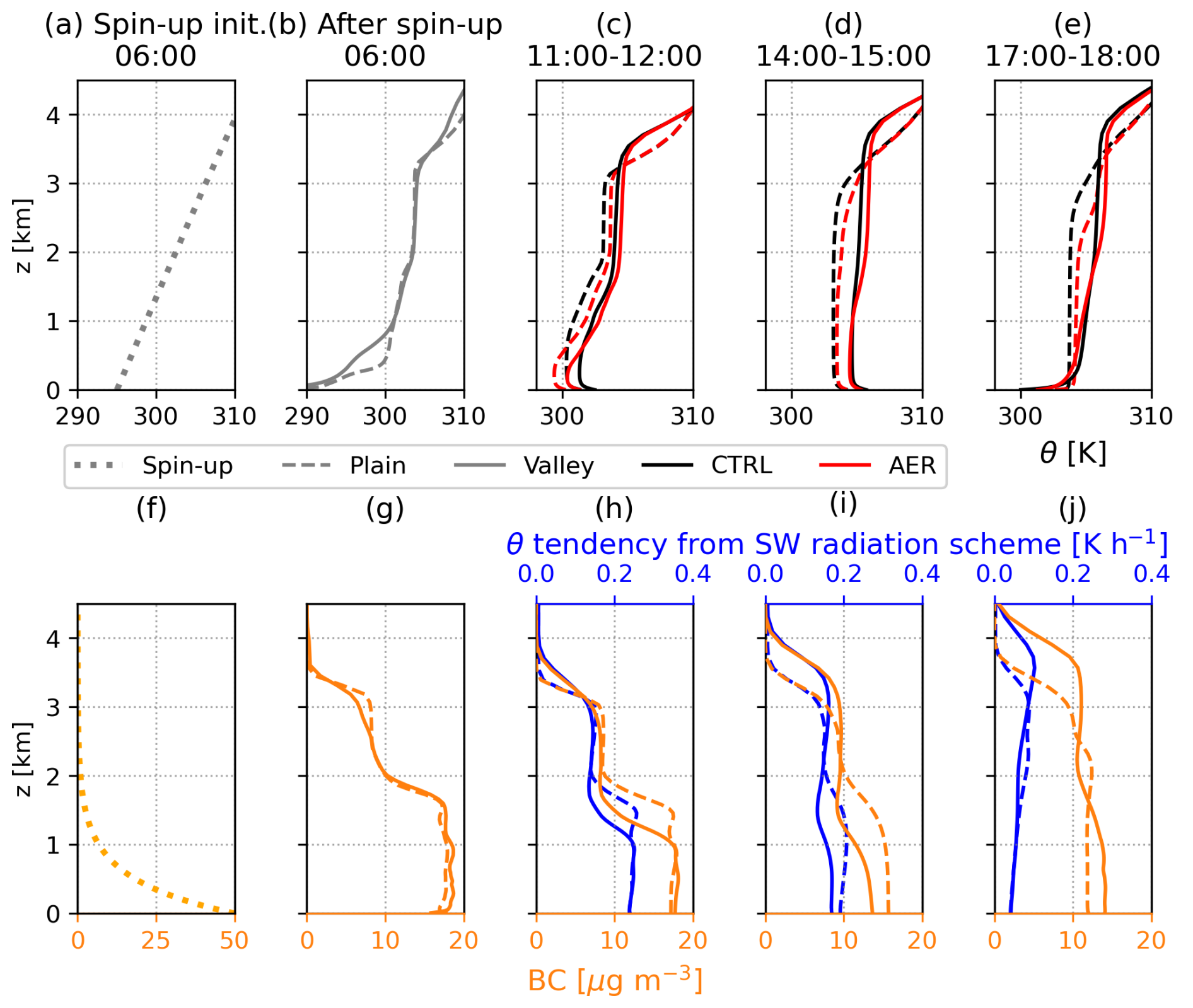
Figure 2 Top row: Vertical profile of potential temperature in both cases AER and CTRL Bottom row: Vertical profile of black carbon and potential temperature tendency from the shortwave radiation scheme in case AER. (a, f) Horizontally uniform initial conditions of the spin-up run. (b, g) Initial condition of the cases AER and CTRL after the 24 h spin-up. Hourly averages between (c, h) 11:00–12:00 (d, i) 14:00–15:00 and (e, j) 17:00–18:00. Solid lines show the vertical profile averaged over the valley centre line (y>0 km, x=0 km) and dashed lines above the plain (y<0 km, x=0 km). Note the different temperature and black carbon concentration scales between the panels and that both cases AER and CTRL have the same spin-up and initial state shown in (a)–(b).

3 Results

3.1 Vertical profiles of BC and potential temperature

Figure 2 shows vertical profiles of potential temperature, BC concentration, and potential temperature tendency from the shortwave radiation scheme, subsequently referred to as the heating rate. The hourly averages are spatially averaged along the centre line of the domain (x=0 km) above the valley (y>0 km, solid lines) and above the plain (y<0,km, dashed lines).

The simulations start at 06:00 from the same initial state as shown in Fig. 2b. The initial state has a stable layer below 1 km and above that there is a less stable layer up to 2 km formed by the nocturnal cooling during the spin-up. Above these stable layers, there is a neutral residual layer that extends up to 3.5 km which was formed during the daytime of the spin-up. In CTRL by midday, a convective surface-based layer up to 0.5 km has developed but above that the stable layer below 2 km still remains (Fig. 2c). In the afternoon at 14:00–15:00, a well developed convective boundary layer reaches up to about 3.5 km above the plain (dashed lines in Fig. 2d) and 4 km above the valley (solid lines). Case AER develops in a very similar manner to case CTRL with 1–2 K colder potential temperatures below 0.5 km and slightly higher potential temperatures (less than 0.5 K margin) above 0.5 km at midday (Fig. 2c). This means the stability below 2 km is stronger in case AER. In the afternoon, case AER has a well developed convective boundary layer up to a similar height as in CTRL with around 1 K higher potential temperatures above 1 km. The convective boundary layer within and above the valley (solid lines) is around 2 K warmer than above the plain (dashed lines) in both simulations. At 17:00–18:00 a surface-based inversion develops in the valley in both simulations, whereas over the plain the near-surface stability is near-neutral (Fig. 2e).

The initial BC profile in case AER has two distinct layers with concentrations around 17 µg m⁻³ below 2 km (Fig. 2g) in the stable layer and concentrations around 8 µg m⁻³ between 2 and 3.5 km. BC concentration decreases rapidly with height above the inversion top at 3.5 km. During the night of the spin-up, BC has accumulated more in the near-surface layer than at higher altitudes (Fig. 2g). This is a result of the nocturnal winds in the valley flowing down the slopes and the surface-based inversion that develop during the night (Fig. 2b), as a similar vertical distribution of BC is found above the plain as well (Fig. 2g). Through the course of the day, the vertical gradient of BC weakens (Fig. 2h–j) as the convective mixing and vertical transport by the valley and slope wind circulation takes place (Sect. 3.2). The well-mixed layer above the valley is deeper and, therefore, BC is mixed in a deeper layer than above the plain (Fig. 2i–j).

The absorption of shortwave radiation by BC in case AER causes a heating rate of up to 0.3 K h⁻¹ at midday (Fig. 2h). The heating rate is on a similar scale to what is reported in previous studies focusing on BC absorption with similar BC concentrations (e.g., Wang et al., 2018; Slater et al., 2022). In case AER, the shortwave heating rate does not increase linearly with the BC concentration (Fig. 2h–j). This is due to less of the incoming solar radiation reaching the lower levels (see Fig. S2a) as absorption by BC occurs above. At midday with the clearly higher BC concentrations below 2 km, the shortwave radiative heating is strongest there (Fig. 2h). In the afternoon when the vertical gradient of BC is weaker, the shortwave heating rate is near equal throughout the well-mixed layer even though the BC concentrations near the surface are still higher than aloft (Fig. 2i–j). The direct radiative effect of BC causes warming rates up to 0.3 K h⁻¹ due to shortwave absorption. However, BC causes a differential heating effect within the boundary layer leading to both cooling and warming at different altitudes. This is seen when the potential temperatures of cases CTRL and AER are compared in Fig. 2c–e. The cooling due to BC below 0.5 km at midday is at most around 2 K above both the valley and the plain (Fig. 2c). In the afternoon in the valley, BC causes warming above 1 km and cooling below 1 km. The simultaneous cooling near the surface and warming of the upper boundary layer means BC makes the boundary layer more stable. Above the plain, the cooling effect near the surface is also seen at midday but in the afternoon the entire boundary layer above the plain is warmed with increasing strength towards the inversion top (Fig. 2i–j). The warming above 1 km is around 1 K with increasing strength towards the inversion top in the afternoon at 15:00 and 18:00 (Fig. 2d–e). Although the BC concentrations are higher at lower levels in the beginning of the day, the effect from BC on the potential temperature profile resembles the dome effect (Sect. 1), in which the stability in the boundary layer is strengthened due to the BC interaction with radiation (e.g., Ding et al., 2016).

3.2 Spatial structure of the daytime valley circulation

Figure 3 shows vertical cross-sections of the v-component of the wind speed (shaded) and potential temperature (black lines) along the valley centre line x=0 km and across y=25 km averaged at 14:00–15:00 for the two simulations. Panels b and d also show the cross-valley wind in x-z-plane as gray vectors. In addition, panels e and f show the BC concentration, and panels g and h show the potential temperature tendency from the shortwave radiation scheme for the case AER.

Daytime plain-to-valley and namely up-valley winds (red colors in Fig. 3a–d) form in both simulations as a result of the temperature difference between the valley atmosphere and the air above the plain below the ridge height of 2 km. The warmer temperatures in the valley compared to over the plain, also seen in the vertical profiles in Fig. 2d, is evident in Fig. 3a, c. Above the up-valley wind layer outside the valley forms the return flow in the down-valley direction (blue colors in Fig. 3a–d). The up-valley winds reach their maximum strength near the valley entrance and decay towards the end of the valley. Qualitatively the spatial structure of the up-valley winds and potential temperature do not differ drastically between the cases CTRL (Fig. 3a–b) and AER (Fig. 3c–d). However, the up-valley winds are stronger in the up-valley jet (0 km $<y<\mathrm{25}$ km) in case AER at the shown time 14:00–15:00 and they extend slightly further into the valley. The two cases develop a surface-based convective boundary layer of similar depth but towards the inversion top the case AER is around 1 K warmer than case CTRL (Fig. 3c, e), which was also seen in Fig. 2d–e.

In the cross-valley direction, up-slope winds form near the heated slopes (Fig. 3b, d). The up-slope winds from both sides converge at the ridge top ($\left|x\right|=\mathrm{10}$ km) resulting in an updraft above the ridge. The cross-valley circulation below the inversion top at 4 km includes also the return circulation away from the slopes and subsidence above the valley centre. Due to the diurnal cycle of solar radiation, there is an asymmetry within the valley as the eastward facing slope receives solar radiation earlier in the day than the westward facing slope. In the afternoon the westward facing slope (shown in Fig. 3b, d) has stronger winds than the eastward facing slope. The up-slope winds flow in a deeper layer in case CTRL (Fig. 3b) than in AER (Fig. 3d). Based on theoretical models (Vergeiner and Dreiseitl, 1987) and real-life observations of up-slope winds (Farina and Zardi, 2023), reduced surface heating and increased stability would both make the up-slope winds weaker and shallower which is in line with Fig. 3b, d. In case AER, the reduction in surface heating stems from the absorption of shortwave radiation by BC within and above the valley. In addition, the heating due to shortwave absorption above the valley increases the stability. Two vertically stacked cross-valley circulation cells separated by an inversion layer (at around z=1.5 km) are seen in case AER (Fig. 3d) but not in case CTRL (Fig. 3b). The formation of such a stacked circulation is favored by increased stability (Wagner et al., 2015b).

Spatial variation of BC in AER is highly influenced by the valley circulation (Fig. 3e–f). The plain-to-valley winds transport BC towards the valley (Fig. 3c, e). From the bottom of the valley centre BC is carried up the slopes and out of the valley by the cross-valley circulation (Fig. 3d, f). The lateral and vertical transport of BC away from the valley centre is seen as a drop in BC concentration along the valley axis (Fig. 3e) when entering from the plain into the valley. Over the plain below 2 km there is less variation in BC in the y-direction. Above the valley the BC layer is deeper than over the plain. Once BC is transported above the valley, the return winds above the ridge height carry some of it towards the plain (Fig. 3c, e). In addition, the convective mixing above the plain causes vertical transport of BC. The subsidence over the centre of the valley by the cross-valley circulation brings cleaner air (i.e. air with lower BC concentration) from above into the valley atmosphere, seen around x=0 km between a height of 1.5 to 2.0 km (Fig. 3f).

Spatial variation in the shortwave heating rate (Fig. 3g–h) is strongly correlated with the BC concentration (Fig. 3e–f). At 14:00–15:00, the strongest shortwave heating occurs where BC concentrations are largest, i.e., below 2 km above the plain, above the ridges, and in the down-valley wind return flow. Similarly, as seen in the averaged vertical profiles (Fig. 2h–j), stronger heating is found at higher altitudes (Fig. 3g–h). The reason is, that due to absorption aloft, less solar radiation reaches the lower levels which leads to weaker heating rate although the BC concentrations are nearly the same.

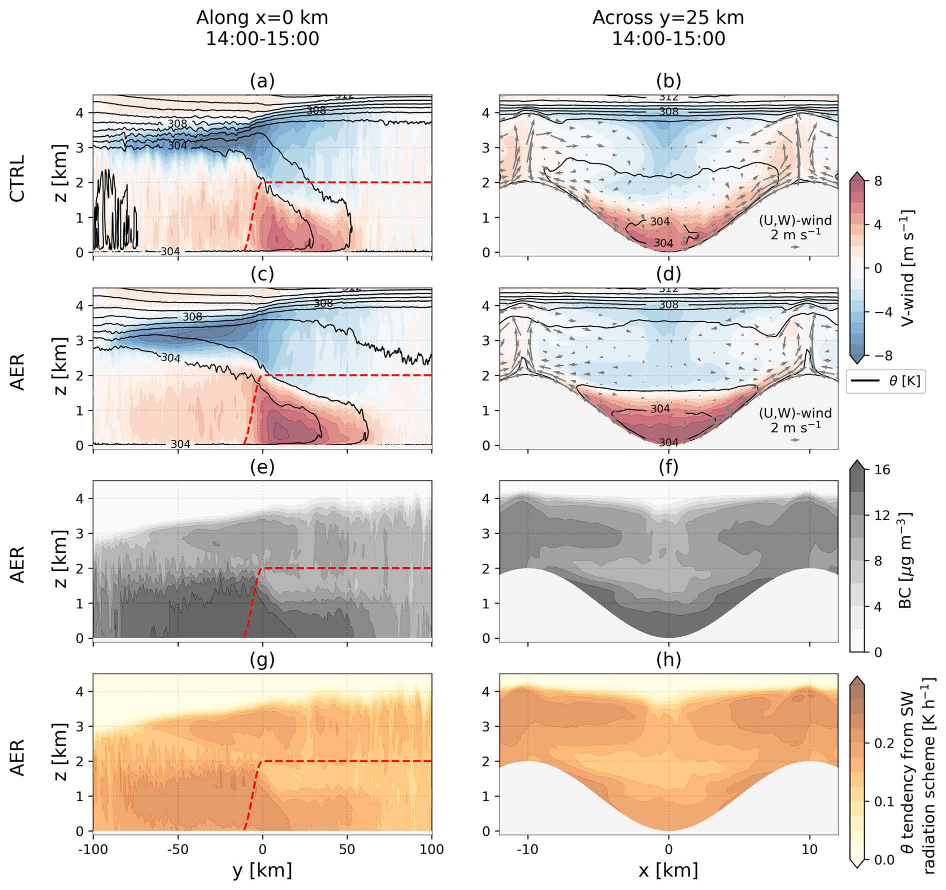
Figure 3 Cross-sections (a, c, e, g) along the valley centre line and (b, d, f, h) across the valley at y=25 km averaged between 14:00 and 15:00. Panels (a)–(b) are from the case CTRL and panels (c)–(h) are from the case AER. (a)–(d) Along-valley wind speed (shaded) and potential temperature (black solid lines). Positive along-valley wind speed refers to up-valley hence right-ward wind in (a), (c). (e–f) Black carbon concentration. (g–h) Potential temperature tendency from shortwave radiation scheme. Red dashed line in (a), (c), (e), (g) show the ridge height at $x=\pm \mathrm{10}$ km.

3.3 Temporal evolution of the valley circulation

Figure 4 shows the temporal evolution of the average v-component of the wind in the valley volume, the u-component of the wind averaged over the lowest 300 m above ground level (a.g.l.) within the valley, and the potential temperature difference between the valley volume and the plain below 2 km. The 2 km reference height above the plain in the potential temperature difference calculation is used to match the ridge height of the valley volume. Positive v-component of the wind refers to up-valley wind. Positive (negative) u-component of the wind on the east (west) slope refers to up-slope wind. Hourly averages are plotted at the end time of each hour and the volume averages are calculated by weighting the individual grid-point values by both density and grid-box volume.

The simulations start at 06:00 with down-valley and down-slope winds that were formed during the night of the spin-up run (Fig. S3). In both simulations, the cross-valley winds in the lowest 300 m above the slopes turn up-slope during the first hour on the west slope (solid line in Fig. 4b) and by 10:00 on the east slope (dashed line). The up-slope winds peak in strength around 13:00 on the west slope and around 16:00 on the east slope. The cross-valley winds turn down-slope on the west-slope around 17:00 and on the east-slope by 19:00. The time lag between the slopes is caused by the diurnal cycle of solar radiation which causes the west slope (east facing) being sun-lit first in the morning and in turn the east slope (west facing) is sun-lit later in the afternoon. The up-slope winds peak in strength between 1.8 and 2.7 m s⁻¹ with some variation between the simulations and the slopes. The up-slope winds are stronger in case CTRL on both slopes. Given the deeper flow layer, the stronger up-slope winds in CTRL would lead to even larger difference in the up-slope mass flux (Fig. S4). The up-slope wind maxima are stronger on the east slope in both simulations.

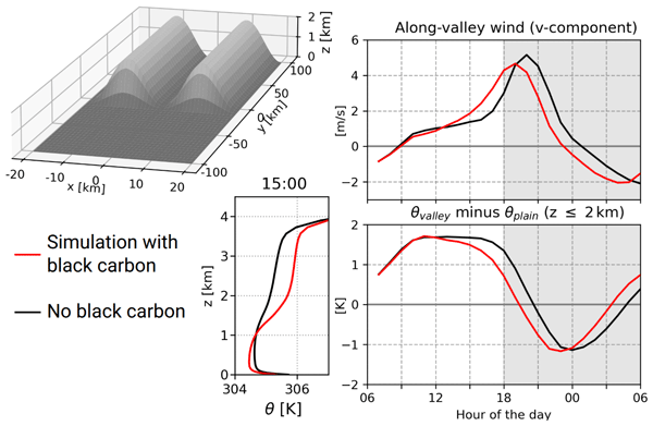
In both simulations, the along-valley wind turns up-valley around 09:00 and reaches the peak strength of around 5 m s⁻¹ in the evening (Fig. 4a). The up-valley winds peak at 19:00 in case AER and at 20:00 in case CTRL. Until midday both cases have similar up-valley wind speeds but between 12:00 and 18:00 case AER has stronger up-valley winds. After the up-valley wind speeds peak at 4.7 m s⁻¹ in AER at 19:00, the case CTRL has stronger up-valley winds with also a higher maximum strength at 5.2 m s⁻¹. The average along-valley wind speed between 12:00 and 20:00 is 2.3 m s⁻¹ in case CTRL and 2.6 m s⁻¹ in case AER. The along-valley winds turn down-valley at 23:00 in case AER and at 01:00 in case CTRL.

As noted in Sect. 3.1 and 3.2, in both simulations the valley atmosphere is warmer than the air above the plain below the ridge height during the day. This is seen from the very beginning of the simulations and the maximum potential temperature difference of approximately 1.6 K is found for both simulations around noon (Fig. 4c). After that, in the case AER the valley-plain temperature difference slowly decays while in the case CTRL it stays near constant until 16:00. Slightly after the up-valley winds peak in strength, the potential temperature difference turns negative, hence the air above the plain becomes warmer than in the valley volume and a few hours later the along-valley winds turn down-valley (Fig. 4a) in both simulations.

An important remark to make is the contradiction between the up-valley wind speeds (Fig. 4a) and the valley-plain potential temperature differences (Fig. 4c). In the afternoon, when the case AER has stronger up-valley winds, the valley-plain potential temperature difference is in fact weaker than in the case CTRL, which is opposite to what the classic valley wind theory states (Sect. 1). According to this theory, the valley-plain potential temperature difference that causes the pressure gradient force between the valley and the plain should be the main driver of the plain-to-valley and up-valley winds. In the following Sect. 3.4, we attempt to explain why the case AER has stronger up-valley winds even with a weaker valley-plain potential temperature gradient.

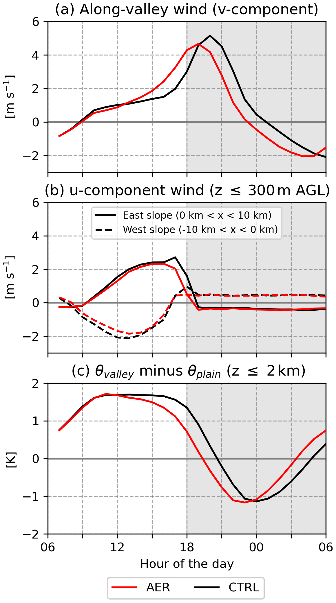
Figure 4 Mass-weighted average of the (a) v-component of the wind in the valley volume (b) u-component of the wind in the nearest 300 m layer from the surface in the valley. (c) Mass-weighted potential temperature difference between the valley volume (y>0 km) and the lowest 2 km above the plain (y<0 km).

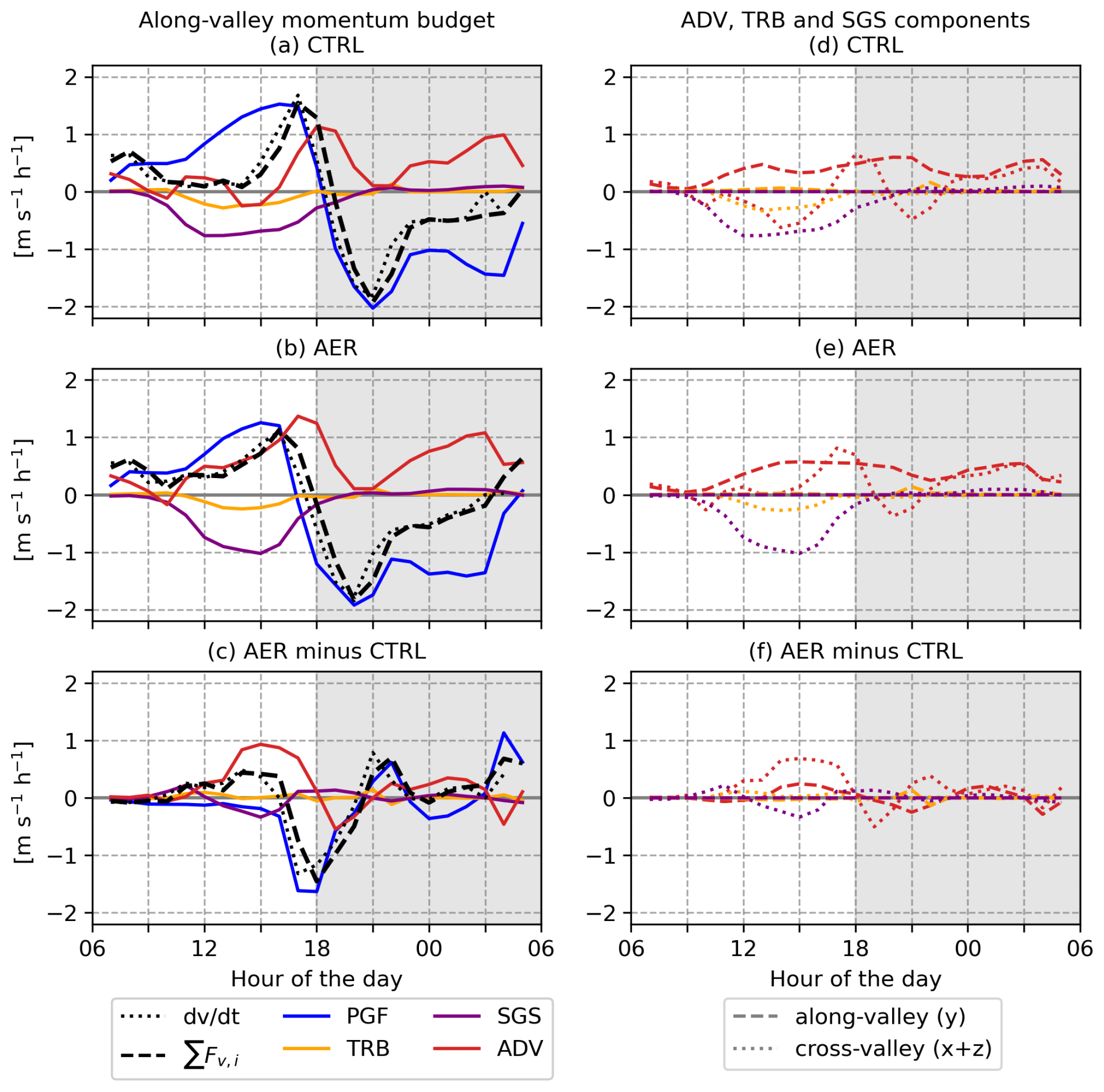
Figure 5 Along-valley momentum budget for the valley volume in (a) CTRL and (b) AER and (c) difference between the two cases. See Sect. 2.2 for details on the budget analysis. Left-hand-side of the Eq. (3) for along-valley momentum is shown on black dotted line and the sum of the terms on the right-hand-side as black dashed line, respectively. (d–f) Same as (a)–(c) but for the tendency due to mean advection, resolved turbulence and sub-grid-scale diffusion decomposed into along and cross-valley components. The cross-valley component includes the vertical one.

3.4 Along-valley momentum budget

Figure 5 shows the temporal evolution of the along-valley momentum budget for the valley volume. For a detailed description of the budget analysis refer to Sect. 2.2. In the left-hand-side panels (a–c), the four terms in the along-valley momentum budget are plotted (see Eq. 1): the pressure-gradient force (PGF), mean advection (ADV), resolved turbulence (TRB), and sub-grid-scale diffusion (SGS). On the right-hand-side panels (d–f) ADV, TRB and SGS are decomposed into the along-valley (y) and cross-valley (x+z) components. Panels (c) and (f) show the difference between the cases AER and CTRL.

The along-valley momentum tendency (black dotted) and the sum of the budget terms (black dashed) show good agreement in both simulations (Fig. 5a–b). This comparison ensures that the momentum budget closes and thus is computed correctly. In case CTRL the net tendency reaches a maximum in the afternoon at 17:00, turns negative around the hour of the peak up-valley winds (Sect. 3.3) at 20:00 and reaches a minimum during the evening transition at 21:00 (Fig. 5a). Schmidli and Rotunno (2012) performed an along-valley momentum analysis for idealised valley simulations. The temporal evolution of the net momentum tendency and the budget terms in their simulation called “periodic” are similar to what is shown for case CTRL in Fig. 5a. The individual terms of both their and our simulation have similar magnitudes. Detailed comparison between case CTRL and the simulation in Schmidli and Rotunno (2012) is not performed as there are major differences in the simulation setup, such as the numerical model, horizontal grid spacing, domain latitude, and valley geometry.

In case AER the net tendency reaches the maximum, turns negative and reaches the minimum one to two hours earlier compared to CTRL (Fig. 5a–b). Overall, the diurnal evolution of the net tendency is similar between the simulations but there are some notable differences in the magnitude, especially from 09:00 until 18:00. Between 10:00 and 15:00 case AER has a stronger positive tendency of the along-valley momentum (Fig. 5a–b) which is in line with the stronger up-valley winds (Sect. 3.3). In contrast, the peak strength in the momentum tendency in case CTRL is higher (Fig. 5a–b), which is again in line with the stronger peak up-valley wind speeds (Sect. 3.3).

In both simulations the PGF has a similar diurnal cycle (Fig. 5a–b) as the valley-plain potential temperature difference (Sect. 3.3), driving the daytime up-valley winds and night-time down-valley winds. The temporal evolution of the PGF is similar between the cases CTRL and AER but with a larger daytime magnitude in CTRL (Fig. 5c) which is in line with the stronger valley-plain temperature difference in CTRL discussed in Sect. 3.3. TRB and SGS reduce the along-valley momentum during the day and have negligible values during the night (Fig. 5a–b). The along-valley component of TRB and SGS (dashed lines in Fig. 5d, e) are negligible low throughout the simulation. TRB and SGS include, for example, tendencies such as the surface drag but also tendency due to turbulent exchange between the valley volume and the surroundings at the valley entrance and at the ridge-top height. TRB shows very similar values for both simulations (Fig. 5c). Along-valley momentum is reduced more by SGS in case AER which can be explained by the higher up-valley wind speeds hence stronger surface drag (z-component included in the cross-valley, Fig. 5d–f).

During the day, the largest difference in the along-valley momentum between the cases AER and CTRL results from the mean advective tendency (ADV, Fig. 5c). In AER, ADV stays positive from 11:00 until the end of the simulation (Fig. 5b) where as in CTRL ADV has negative values in the afternoon from 13:00–16:00. During daytime, positive ADV would refer to advection of air with high along-valley momentum at the valley entrance by the plain-to-valley winds (Sect. 3.2), which is seen as positive values of the ADV along-valley component (dashed line in Fig. 5d, e). Interestingly, in CTRL the daytime cross-valley circulation reduces the along-valley momentum (negative values, dotted line in Fig. 5d) as the up-slope winds carry air with high along-valley momentum (i.e. up-valley winds) vertically out of the valley volume at the ridge height. This is also seen in the cross-section in Fig. 3b as there are up-valley winds outside the valley volume above the ridge height which may be interpreted as a direct consequence of a vertical transport of along-valley momentum. In addition, the return flow and subsidence above the valley centre bring air with low or down-valley momentum into the valley volume from above which reduces the up-valley momentum. However, in the case AER the export of up-valley winds/import of down-valley winds by the cross-valley circulation is weak or even absent between 10:00 and 15:00 (Fig. 5e). In case AER, up-valley winds are seen above the ridge in Fig. 3d at 15:00, but much weaker than in the case CTRL. The transport by TRB and SGS may also contribute in the export of along-valley momentum, but the most striking difference between the simulations are found in the mean advective part (Fig. 5c, f).

3.5 Heat budget

Figure 6 shows the temporal evolution of the heat budget for the valley volume (see Eq. 2). The heat budget involves a resolved mean advective term (ADV), a resolved turbulent term (TRB), a sub-grid-scale diffusion term (SGS) which involves the surface sensible heat flux, and the heating tendencies due to shortwave (RSW) and longwave radiation (RLW).

Similar to the momentum budget, the sum of the budget terms (black dashed) and the independently computed heat tendency (black dotted) show a good agreement throughout the simulations (Fig. 6a, b), indicating that the budget is closed. In both simulations, the warming is strongest at midday and the valley volume starts cooling two hours before sunset around 16:00. The strongest cooling occurs around 18:00 during the evening transition and decays with time during the night. In case CTRL, the net heat tendency in the valley volume and the individual heat-budget terms exhibit a diurnal-cycle shape and magnitude similar to those reported by Schmidli and Rotunno (2012), who performed a comparable heat-budget analysis for their idealised valley simulation, “periodic”.

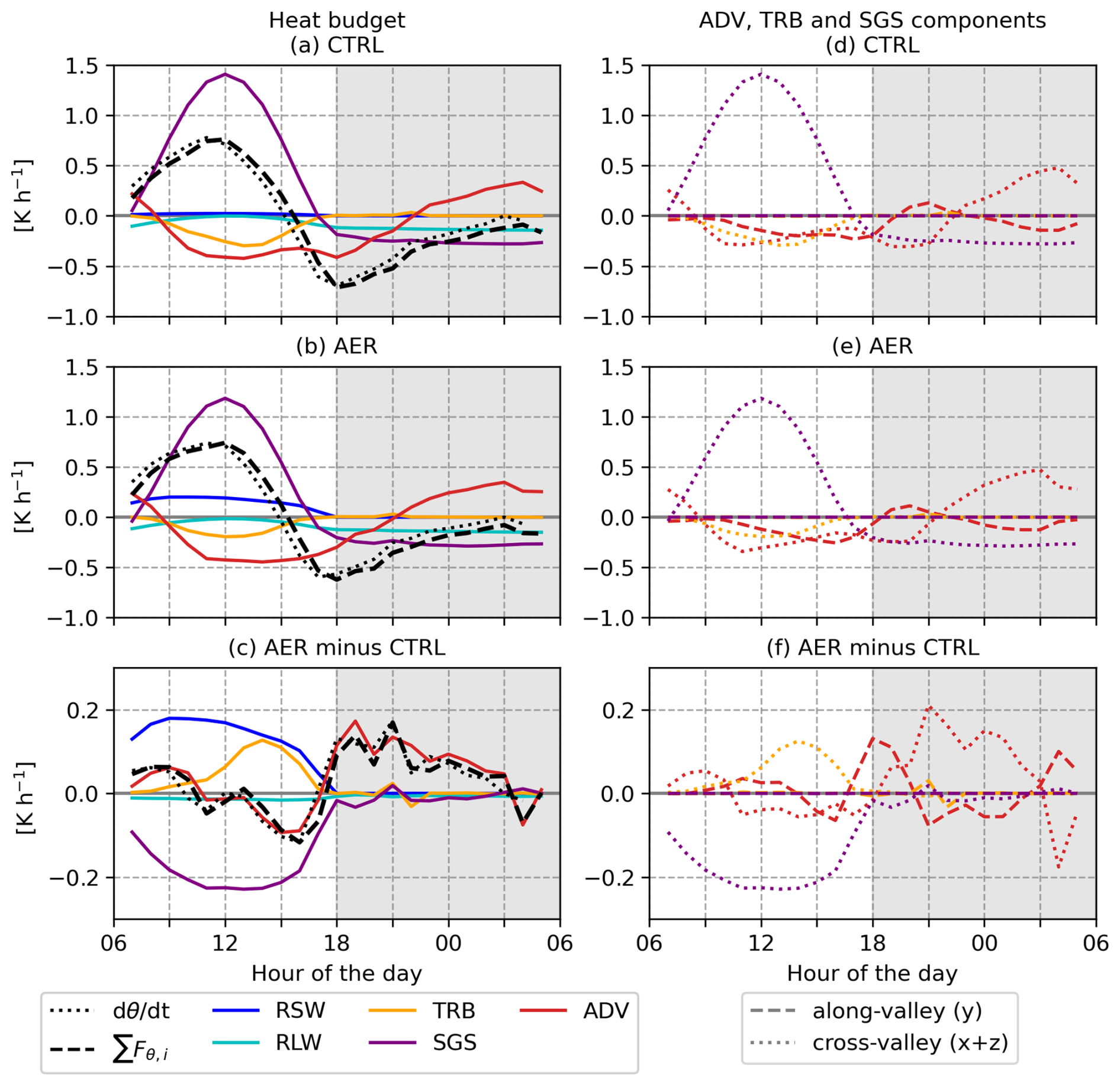
Figure 6 Heat budget for the valley volume in (a) CTRL and (b) AER and (c) difference between the two cases. See Sect. 2.2 for details on the budget analysis. Left-hand-side of the Eq. (3) for heat is shown on black dotted line and the sum of the terms on the right-hand-side on black dashed line, respectively. (d–f) Same as (a)–(c) but for the tendency due to mean advection, resolved turbulence and sub-grid-scale diffusion decomposed into along and cross-valley components. The cross-valley component includes the vertical one.

The mean daytime valley circulation acts to cool the valley volume, seen as negative ADV in Fig. 6a–b. This includes import of cold air at the valley entrance by the plain-to-valley winds (ADV along in Fig. 6d, e), and export of warm air at the ridge-top height by the up-slope winds (ADV cross in Fig. 6d, e). During the evening transition, the net tendency turns negative before sunset as the heating from the solar radiation weakens and the prevailing daytime valley circulation cools the valley volume (Fig. 6a, b).

Sub-grid-scale diffusion (SGS) shows a clear diurnal cycle with a peak at noon and a constant negative tendency during the night (Fig. 6a, b). In case AER there is heating due to shortwave radiation (RSW) during the day with a heating rate less than 0.2 K h⁻¹ in the valley volume. RSW has the strongest values at 10:00–11:00. This is probably due to BC ventilation out of the valley volume by the daytime cross-valley circulation (Sect. 3.2). Earlier in the day, more BC is located in the valley volume compared to above the valley (Fig. 2h–j). As the BC is transported out of the valley, the heating due to BC absorption occurs more and more outside the valley. This reduces the shortwave radiation aloft, hence, there is both less shortwave radiation and less BC mass in the valley volume.

When comparing the two simulations in Fig. 6c, f, the reduction in SGS due to the BC absorption is stronger than the positive heat tendency due to RSW in the valley volume. The surface heating (SGS) is reduced as the absorption by BC reduces the incoming solar radiation reaching the ground. However, the absorption occurs also above the valley (Sect. 3.1–3.2), not only within the valley volume for which the heat budget is computed. This leads to a reduction in the shortwave radiation reaching the top of the valley volume in case AER when compared to the case CTRL (Fig. S2a). The unequal heat input from shortwave radiation leads to asymmetry between the reduction of heating by SGS and the increase of heating by RSW. However, the difference in TRB seems to even out the asymmetry between SGS and RSW as the net difference between the simulations follows very closely the ADV term (Fig. 5c). All of the TRB comes from the cross-valley component (Fig. 6f) which would mean a weaker export of heat at the valley top in AER in the afternoon. The temporal evolution of ADV in the along and cross-valley directions look qualitatively very similar between the simulations (Fig. 6d, e) with the one to two hour time lag in the evening transition. The stronger negative values in the along-valley component of ADV in case AER in the afternoon might be caused by the stronger plain-to-valley winds, however, the weaker valley-plain potential temperature difference would compensate this. Throughout the day, the export of heat by the cross-valley component of ADV is stronger in case CTRL than in case AER. This is likely caused by the reduced surface heating and increased stability due to the shortwave absorption by BC leading to weaker up-slope winds in case AER (Sect. 3.2–3.3).

4 Conclusions

The impact of black carbon (BC) on daytime valley and slope winds was studied by means of high-resolution WRF-Chem simulations with idealised valley topography. The study consists of two 24 h-long simulations that start from the same initial conditions that have been achieved by a 24 h spin up. One simulation, referred to as AER, has realistic BC concentrations affecting the thermodynamic and kinematic structure of the atmosphere mainly through the absorption of incoming solar radiation. The reference simulation, referred to as CTRL, is run without the effects of BC and, hence, the aerosol-meteorology feedback is switched off.

During daytime BC alters the potential temperature by warming the top of the boundary layer above 1 km and cooling the levels below 1 km. The absorption aloft leads indeed to reduced surface heating in case AER as less solar radiation reaches the ground. Warming above and cooling at lower levels means the stability in the boundary layer is stronger in case AER. The reduced surface heating and higher boundary layer stability leads to weaker up-slope wind speeds in the case AER. Between 13:00 and 19:00 the case AER has stronger up-valley winds than the case CTRL, although the potential temperature difference between the valley atmosphere and the air above the plain is weaker. Based on the classic valley wind theory, the weaker potential temperature difference and associated weaker pressure-gradient force should result in weaker up-valley winds, which is not the case in our simulations.

To disentangle this counterintuitive result, along-valley momentum and heat budgets were computed for the valley volume using the WRFlux-tool. The momentum budget analysis shows that although the daytime pressure-gradient forcing is stronger in case CTRL, the net momentum tendency is higher in case AER mainly due to weaker export of along-valley momentum by the cross-valley circulation. In case CTRL, the daytime up-slope winds transport air with high along-valley momentum (i.e. up-valley winds) vertically out from the valley. In contrast, with the weaker up-slope winds in case AER due to reduced surface heating and higher stability in the valley atmosphere, less along-valley momentum is exported out of the valley volume. This allows stronger up-valley winds to develop in the afternoon in case AER although the pressure-gradient forcing is stronger in case CTRL. However, in the evening the maximum up-valley winds are stronger in case CTRL. The heat budget analysis shows that the difference between the simulations in the net heat tendency follows closely the difference in the heat tendency due to the mean advection. Throughout the day and the evening transition, the mean flow advection acts to cool the valley volume in both cases. The warming in the valley volume due to absorption of shortwave radiation by BC in case AER is weaker than the reduction of heat flux from the surface. This is likely due to the valley volume in case AER receiving less solar radiation as BC absorption occurs also above the valley volume.

The daytime up-valley winds in case CTRL exhibit magnitudes comparable to those found in previous studies using similar idealised model experiments (e.g. Schmidli and Rotunno, 2010; Wagner et al., 2015a). The heat and momentum budgets also exhibit similar diurnal behavior and are a similar order of magnitude as what Schmidli and Rotunno (2012) found in their budget analysis of similar idealised simulations. Results from our simulations show that realistic BC concentrations can alter the development of the daytime valley and slope winds. The average along-valley wind speed between 12:00 and 20:00 is 2.6 m s⁻¹ in AER and 2.3 m s⁻¹ in CTRL. In the evening the maximum up-valley winds are stronger in case CTRL by a margin of 0.5 m s⁻¹. The impact of BC on the daytime up-valley wind speed is notable, but still relatively weak compared to the impact of the valley geometry (e.g. width, along-valley heterogeneity, valley floor inclination, Schmidli and Rotunno, 2015; Wagner et al., 2015a, b; Mikkola et al., 2025), the topography surrounding the valley (Schmidli and Rotunno, 2012), or the thermal forcing and stability of the atmosphere (Schmidli and Rotunno, 2015).

Although the BC concentrations in AER are realistic for polluted urban area, like Kathmandu in the Himalayan foothills (Putero et al., 2018) or Milan in the Po valley (Ferrero et al., 2014), in the real atmosphere BC is only one component in the anthropogenic aerosol particulate matter. Other aerosol compounds with absorbing and scattering properties do influence boundary-layer processes as well (Ma et al., 2020; Slater et al., 2022). Results from our simulations show the effect of only one absorbing aerosol compound, revealing a mechanism which affects the thermally-driven winds in a mountain valley. Previous studies focusing on the atmosphere above flat ground have shown that the impact of aerosols on boundary-layer processes is sensitive to the properties and vertical distribution of the aerosol population (Sect. 1). Further work on the topic could include increased number of model experiments, for example, with different initial aerosol distribution (higher or lower concentrations, shape of the vertical profile), different valley topographies (i.e. valley inclination), different thermal forcing (i.e. latitude and orientation of the domain), and including other chemical compounds with scattering as well as absorption properties. Other aspects that could be studied with a similar model setup to ours include the ventilation of BC into the free troposphere and deposition of BC in the valley topography.

Appendix A: Sensitivity of model output to horizontal resolution

Sensitivity of the model results is tested with an additional simulation with a horizontal grid spacing of 100 m and a time step of 1 s. The model configuration of the additional simulation is identical to the case CTRL apart from the horizontal grid spacing, time step, and a change in the domain width. Due to computational limits, the domain width in the cross-valley direction was decreased to 20 km so that the model x boundaries are located at $x=\pm \mathrm{10}$ km (at the ridge-top). As the lateral boundaries in x direction are periodic, the model topography in practice remains the same in the sensitivity run, as the domain length in the along-valley direction did not change.

The decrease of the horizontal grid spacing and time step to half of the original has a negligible influence on the model results. The general structure of the daytime up-valley winds are qualitatively very similar between the two simulations, shown in the Fig. S5. The temporal evolution of the valley-volume-averaged winds and the temperature contrast between the valley volume and the air above the plain show very minimal difference in the sensitivity simulation when compared to CTRL, shown in the Fig. S6. Similarly, very minor changes in the ADV, TRB and SGS tendencies are seen in the along-valley momentum and heat budget analyses, shown in the Figs. S7 and S8. This sensitivity test gives confidence for the use of the simulations CTRL and AER to study the impact of black carbon on the valley circulation and associated exchange processes. Wagner et al. (2015b) found similar result for their model sensitivity test in idealised valley simulations. Our results are consistent with those of Wagner et al. (2015b), who also found negligible differences between their simulations with 200 and 100 m grid spacing.

Appendix B: Idealised valley topography

The idealised valley topography is defined following Wagner et al. (2015a), Schmidli and Rotunno (2010), and Mikkola et al. (2025). The topography is defined by Eq. (B1)

$$\begin{array}{}\text{(B1)}& h(x,y)=R_s{h}_r\left(y\right)\left({\displaystyle \frac{\mathrm{1}}{\mathrm{2}}}-{\displaystyle \frac{\mathrm{1}}{\mathrm{2}}}\cos \left(\mathit{\pi }{\displaystyle \frac{\left|x\right|}{S_x}}\right)\right),\end{array}$$

where R_s is the valley depth (R_s=2 km in this study), S_x is the half-width of the valley (i.e. the length of the slope in the x-direction, S_x=10 km in this study), and h_r(y) is the along-valley height profile of the ridge at $x=\pm S_x$. The profile along the ridges is defined by

$$\begin{array}{}\text{(B2)}& h_r\left(y\right)=\left\{\begin{array}{ll}\mathrm{0},& y\le -S_y\\ \frac{\mathrm{1}}{\mathrm{2}}+\frac{\mathrm{1}}{\mathrm{2}}\cos \left(\frac{\mathit{\pi }}{S_y}y\right)& -S_y<y<\mathrm{0}\\ \mathrm{1}& y>\mathrm{0}\end{array}\right.,\end{array}$$

where S_y is the length in the y-direction over which the ridges increase in height to their full depth at the valley entrance (S_y=12 km in this study).