Thirty years of arctic primary marine organic aerosols: patterns, seasonal dynamics, and trends (1990–2019)

Changing Arctic climate conditions have accelerated sea ice retreat, altering ocean–atmosphere interactions and marine ecosystems. Reduced sea ice cover likely enhances emissions of primary marine organic aerosol (PMOA) through bubble bursting, with implications for aerosol–cloud interactions. This study examines the emission patterns, seasonality, and historical trends of key PMOA species (dissolved carboxylic acidic containing polysaccharides, PCHO; dissolved combined amino acids, DCAA; polar lipids, PL) within the Arctic from 1990 to 2019. Surface ocean concentrations of marine biomolecules, derived from a biogeochemistry model used in the ECHAM-HAM aerosol–climate model, exhibit pronounced seasonal cycles. PMOA emissions show strong variability, driven by marine productivity and sea-salt emissions, with maxima from May to September. Total PMOA emissions increased by about 12 %, and the burden rose by 4 % between 1990–2004 and 2005–2019. A 30 year summer trend (July–September) indicates a rapid decline in sea ice, accompanied by increasing concentrations of organic groups in inner-Arctic waters. Positive PMOA emission anomalies have become more frequent over the past 15 years, and total PMOA production has increased by 0.8 % yr⁻¹ since 1990. Differences among biomolecular types persist, with PCHO showing the strongest increases in both emissions (1.3 % yr⁻¹) and aerosol concentrations (0.8 % yr⁻¹).

1 Introduction

The Arctic region is undergoing drastic changes as surface air temperatures are increasing more rapidly than those for the rest of the world (Wendisch et al., 2019; Rantanen et al., 2022; Wendisch et al., 2023). This phenomenon, known as Arctic amplification, is driven by several feedback mechanisms (Block et al., 2020; Wendisch et al., 2023). One key process is the sea ice–albedo feedback, in which the decline of highly reflective sea ice and snow surfaces contributes to further warming and melting sea ice (Serreze and Barry, 2011). Particularly, the unprecedented decline in sea ice area over the past 30 years presents an urgent call for research (Johannessen et al., 2004). Since the positive ice-albedo feedback mechanism in the Arctic has contributed to warming the ocean, the open water season has consequently extended (Perovich et al., 2007; Stammerjohn et al., 2012; Arrigo and van Dijken, 2015). The retreating sea ice also impacts the marine biological activity by a complex chain of processes linked to light availability, fresh nutrient supply and vertical mixing (Ardyna and Arrigo, 2020; Nöthig et al., 2020). As a result, the distribution and magnitude of phytoplankton blooms, as well as the duration of the growing season, have notably changed in the last decades (Arrigo et al., 2008; Arrigo and van Dijken, 2011; Ardyna and Arrigo, 2020). These factors modify the total primary production and determine regional differences within the Arctic (Arrigo et al., 2008; Kahru et al., 2011; Aksenov et al., 2011; Fernández-Méndez et al., 2015; Cherkasheva et al., 2025).

This likely also affects the Arctic aerosol burden, which has a significant contribution from local marine sources (Moschos et al., 2022). Here, sea spray aerosol, primarily generated through bubble bursting of breaking waves driven by wind action on the sea surface, is a major contributor during the Arctic summer (Leck et al., 2002; Deshpande and Kamra, 2014; Heintzenberg et al., 2015; Willis et al., 2017; Lawler et al., 2021; Gu et al., 2023). Organic surfactants present in seawater attach to rising bubbles and are released into the atmosphere together with sea salt (Facchini et al., 2008; Keene et al., 2007; Gantt et al., 2011; Gantt and Meskhidze, 2013). The organic particles originated through this mechanism are known as primary marine organic aerosol (PMOA) (Facchini et al., 2008; Gantt et al., 2011; de Leeuw et al., 2014). As a result of the changing climate conditions, the melting sea ice leads to new, extensive areas of open water and ice fractures, where wind-driven sea spray emissions could occur. Additionally, the relationship between PMOA production and the release of ocean surface organic components through biological processes suggests that variations in marine productivity could affect the marine aerosol emissions. This, in turn, potentially has far-reaching consequences for aerosol–cloud interactions and associated climate effects in the Arctic.

Observations have widely documented the important role of local marine sources (Russell et al., 2010; Frossard et al., 2014; May et al., 2016; Kirpes et al., 2019; Lawler et al., 2021; Zeppenfeld et al., 2019, 2023; Rocchi et al., 2024) and the relevance of PMOA for cloud formation in the Arctic (Leck and Bigg, 2005a; Bigg and Leck, 2001b; Irish et al., 2017; Hartmann et al., 2021; Creamean et al., 2022; Porter et al., 2022). The presence of marine organics in aerosol has been linked to marine biological activity as a correlation with phytoplankton proxies (chlorophyll a) and measured organic compounds in seawater (Leck and Bigg, 2005a; O'Dowd et al., 2008; Russell et al., 2010; Rinaldi et al., 2013; May et al., 2016; Zeppenfeld et al., 2023). In addition, the capability of PMOA to act as cloud condensation nuclei (CCN) has been explained by the strong dependence found between CCN population and insoluble organic aerosols linked to the composition of the marine surface microlayer (the top-most ocean layer at the ocean-atmosphere interface) (Leck and Bigg, 2005a). Moreover, repeated evidence of biological ice nucleating particles (INP) in relation to local marine emissions in the Arctic and at Nordic Seas stations has been extensively reported (Wilson et al., 2015; Irish et al., 2017; Creamean et al., 2019; Wilbourn et al., 2020; Hartmann et al., 2021; Creamean et al., 2022; Porter et al., 2022; Sze et al., 2023).

The representation of PMOA emissions in aerosol–climate models considers the same principles found in observations. Available emission parametrizations for estimating the organic mass fraction in sea spray, follow either a chl a based empirical formulation (O'Dowd et al., 2008; Gantt et al., 2011; Rinaldi et al., 2013) or an organic-class-resolved approach that accounts for the physicochemical characteristics of ocean biomolecules (Burrows et al., 2014). Both types of schemes have been implemented and evaluated in global models (Gantt and Meskhidze, 2013; Huang et al., 2018; Zhao et al., 2021; Leon-Marcos et al., 2025). Nonetheless, the analysis of the PMOA as species-resolved organic groups (e.g, polysaccharides, proteins, and lipids) could provide additional evidence of potential differences in marine organic aerosol abundance. Recent findings from Arctic measurements confirm the high enrichments of carbohydrates in aerosols, which were also detected in the surface microlayer of the marginal ice zone and in aged melt ponds (Zeppenfeld et al., 2023). This supports previous findings by Russell et al. (2010) of saccharide compounds in Arctic marine aerosols. Similarly, a notable contribution of glucose, which could be considered as a proxy for ice nucleating activity (Zeppenfeld et al., 2019), has been measured in sea spray aerosol north of 80° N (Rocchi et al., 2024). In addition to carbohydrate-like substances, Hawkins and Russell (2010), also found evidence of marine proteinaceous material in aerosol particles. Lipid-like molecules (e.g. n-alkanes and fatty acids) have also been analysed in the Bering Sea, with significant contributions to marine aerosols in summer (Hu et al., 2023). Therefore, the critical role of PMOA emissions, transport patterns and evolution under the rapidly changing climate should be thoroughly studied for individual species.

The effect of retreating Arctic sea ice on sea spray emissions has been discussed to some extent, and model results point to an increase in sea salt aerosol concentration in the following decades (Struthers et al., 2011; Gilgen et al., 2018; Lapere et al., 2023). In light of the increasing fraction of sea ice cracks, leads, melt ponds and the marginal ice zone (Rolph et al., 2020; Zhang et al., 2018; Willmes and Heinemann, 2015), they are currently considered a relevant source of local emissions via bubble bursting (May et al., 2016; Kirpes et al., 2019; Lapere et al., 2024). Insights on the organic contribution from these marine sources have been provided in recent studies (Kirpes et al., 2019; Zeppenfeld et al., 2023; Wang et al., 2024). Nevertheless, the spatio-temporal distribution among organic compounds in water bodies is not uniform and strongly depends on the marine biological origin of the considered biomolecule groups in seawater (Burrows et al., 2014; Leon-Marcos et al., 2025). Furthermore, the interplay between marine sources and the loss of sea ice, as well as their relevance for PMOA and mixed-phase clouds, and thus, for the climate in the Arctic, remains unclear (Wendisch et al., 2023). To a large extent, this is due to remaining uncertainties and limitations in the understanding and representation of the life cycle and aerosol–cloud effects of PMOA in aerosol–climate and Earth System Models (ESM) (Taylor et al., 2022). Based on observational evidence of marine biogenic INP particles predominance, their consideration in ESM will potentially improve the model representation of clouds (Schmale et al., 2021).

Given the biomolecule physicochemical characteristics, some groups are selectively aerosolised (lipids), whereas others have higher INP potential (polysaccharides and proteins) (Facchini et al., 2008; Burrows et al., 2014; Alpert et al., 2022). Such disparities are pronounced in the Arctic by the complex dynamical changes of sea ice and atmospheric conditions. Hence, the response of PMOA species abundance and indirect climate impact presumably responds differently to changes in the fragile marine ecosystem. Understanding how marine biomolecules and their organic contributions to aerosols have evolved under the changing Arctic climate is therefore essential. To our knowledge, however, a species-resolved trend analysis of marine organic groups in seawater and aerosols has not been performed.

In this study, we aim to unravel how the interplay of emission drivers has determined the evolution of PMOA species within the Arctic circle (66–90° N) from 1990 to 2019. For the simulation experiments, we use the model configuration as described in Leon-Marcos et al. (2025) for the aerosol–climate model ECHAM6.3-HAM2.3 (Tegen et al., 2019). As relevant for the PMOA emissions, the following highly abundant biomolecule groups in seawater are taken into account (dissolved carboxylic acidic containing polysaccharides, PCHO; dissolved combined amino acids, DCAA; and polar lipids, PL) as introduced by Leon-Marcos et al. (2025). The OCEANFILMS (Organic Compounds from Ecosystems to Aerosols: Natural Films and Interfaces via Langmuir Molecular Surfactants; Burrows et al., 2014) scheme, recently implemented into the ECHAM-HAM model, allows for accounting for the organic fraction of these groups in nascent sea spray and simulating the aerosol transport, transformation, and removal processes.

2 Methods

This study examines the patterns, seasonal dynamics, and trends of primary marine organic aerosols (PMOA) in the Arctic region using results from a comprehensive marine biogeochemical model that simulates key oceanic biomolecules and their associated production and sink processes. These results are used in simulations of a global aerosol–climate model to represent emissions and transport of PMOA, focusing specifically on key species groups. The detailed technical description of the associated model development, configuration, and input data is provided by Leon-Marcos et al. (2025). All abbreviations referring to marine groups and aerosol components are in accordance with the definitions by Leon-Marcos et al. (2025) and are listed in Table A1. This analysis spans a 30 year period (1990–2019), offering insights into the temporal and geographical characteristics of Arctic PMOA.

2.1 The aerosol–climate model ECHAM-HAM

The atmospheric simulations for this study are performed with the global state-of-the-art aerosol–climate model system ECHAM-HAM (version ECHAM6.3-HAM2.3; Tegen et al., 2019). ECHAM simulates atmospheric circulation and dynamics while aerosol microphysics and transport are modelled by the Hamburg Aerosol Module (HAM; Stier et al., 2005; Zhang et al., 2012), which is online coupled to ECHAM. HAM is based on the M7 aerosol model (Vignati et al., 2004) that represents aerosols as soluble or insoluble modes, comprising seven log-normal classes that fall into a size spectrum of four categories depending on the particle radius (r): nucleation (r≤ 0.005 µm), Aitken (0.005 µm < r≤ 0.05 µm), accumulation (0.05 µm < r≤ 0.5 µm) and coarse modes (r > 0.5 µm). The model includes several aerosol species such as sulphate (SO₄), organic carbon (OC), black carbon (BC), mineral dust (DU) and sea salt (SS), which were evaluated by Tegen et al. (2019). Leon-Marcos et al. (2025) implemented PMOA species in the model as additional tracers in the accumulation size mode and performed a thorough evaluation of the model results. PMOA emissions are based on the premise that marine organic matter is co-emitted with SS as sea spray. Hence, the mass (M) of sea spray can be calculated as $M\left(\text{sea\hspace{0.17em}\hspace{0.17em}spray}\right)=M\left(\text{PMOA}\right)+M\left(\text{SS}\right)$. Consequently, the estimated emission mass flux of PMOA groups (PMOA_{mass  flux}) can be derived from that of sea salt (SS_{mass  flux}), given the fraction that organics represent of sea spray:

$$\begin{array}{}\text{(1)}& {\text{PMOA}}_{\text{mass\hspace{0.17em}\hspace{0.17em}flux}}\left(i\right)={\displaystyle \frac{{\text{SS}}_{\text{mass\hspace{0.17em}\hspace{0.17em}flux}}\times {\text{OMF}}_i}{\mathrm{1}-{\text{OMF}}_i}},\end{array}$$

where SS_{mass  flux} in the model is calculated based on the Long et al. (2011) source function, considering a surface temperature correction in accordance with Sofiev et al. (2011). OMF_i is the organic mass fraction of each biomolecule group i obtained from the parameterization OCEANFILMS (Burrows et al., 2014) that has been recently included as part of the PMOA implementation.

2.2 Source representation of primary marine organic aerosol

The OCEANFILMS parameterization represents the transfer of marine organics to the atmosphere (Burrows et al., 2014). It estimates the organic mass fraction in nascent sea spray aerosols of various organic groups. The scheme is based on the Langmuir isotherm model, which represents the differential absorption of organics at the bubble surface. Each group is characterised by distinct physicochemical properties that will determine their transfer to the aerosol phase. The aerosolisation of these marine organics occurs in a chemoselective manner, in which the compounds with higher surface affinity, such as lipids, are preferably transferred. Other molecules that possess a lower surface affinity, such as proteins, polysaccharides, humic and processed compounds, are also considered in OCEANFILMS. However, only three groups are included in this study: lipids, polysaccharides, and protein-like mixtures. Excluding the other groups that originate from the recalcitrant portion of dissolved organic carbon (DOC) in seawater has a negligible effect on the aerosol organic mass fraction (Burrows et al., 2014). A more extensive explanation of the model characteristics, the methodology employed to compute the biomolecules, and the evaluation against seawater samples can be found in Leon-Marcos et al. (2025).

2.2.1 Ocean biomolecule concentration

As lower boundary conditions for the OCEANFILMS scheme in ECHAM-HAM, we use simulation results from the Regulated Ecosystem Model (REcoM, version 3) coupled to the general circulation and sea-ice Finite VolumE Sea-ice Ocean Model (FESOM, version 2.1) (Gürses et al., 2023). FESOM-REcoM simulates globally the ocean dynamics and marine biogeochemistry, respectively. REcoM includes two types of phytoplankton and zooplankton, as well as nutrients, dissolved and particulate organic matter, and debris (Oziel et al., 2025). Phytoplankton metabolism, such as carbon exudation, is controlled by non-linear limiting functions based on the intracellular nitrogen-to-carbon ratio (Geider et al., 1998; Schourup-Kristensen et al., 2014). The FESOM employs an unstructured grid, enabling higher resolution in dynamically active regions, such as the Arctic. For the present investigation, we utilise monthly values of the FESOM-REcoM simulations, which were interpolated to a regular grid with a horizontal resolution of 30 km. Furthermore, a volume-weighted average over the top 30 m of the water column, as in Zeising et al. (2025), is used to represent the marine tracers at the ocean surface.

Based on REcoM model tracers, Leon-Marcos et al. (2025) developed a closure approach to simulate the highly abundant biomolecule groups in seawater. The approach considers the main products of dissolved organic carbon exuded by phytoplankton (DOC_{phy_ex}). This fraction of the DOC is apportioned into the contribution of different biomolecule groups, in addition to a residual. The main biomolecules in seawater considered are dissolved carboxylic acidic containing polysaccharides (PCHO_sw), dissolved combined amino acids (DCAA_sw) and polar lipids (PL_sw). Any compound that does not belong to the aforementioned groups is attributed to the residual.

The ocean concentrations of the biomolecular groups are calculated using different methods. PCHO is computed online as a tracer in the current REcoM model (Zeising et al., 2025), representing a significant portion of exuded carbon (63 %, Engel et al., 2004; Schartau et al., 2007). PCHO_sw aggregation product is also computed as a sink term and considered an additional model tracer (Transparent Exopolymer Particles, TEP).

On the other hand, PL_sw is calculated offline and accounts for a small fraction of DOC_{phy_ex} (5 %). The calculation for the PL_sw group incorporates the phytoplankton carbon exudation rate over a short timescale of a few days, accounting for its role as a semi-labile compound. Lastly, DCAA_sw is estimated as a fraction of modelled PCHO_sw. This fraction refers to the ratio derived from analogous compounds of these two groups in seawater samples. As measurements are incapable of distinguishing between biomolecule sources in the ocean, the computed DCAA_sw concentration may encompass other sources besides phytoplankton carbon exudation. Hence, as PCHO_sw corresponds to the semi-labile group in the ocean, with turnover periods spanning from months to years, the calculated DCAA_sw will also be included in this portion. The offline precalculated ocean concentrations of the three biomolecule groups are finally provided as input files for the marine emission scheme in the ECHAM-HAM model.

2.2.2 Experimental model setup

The simulations of PMOA were conducted with ECHAM-HAM for the 30 year period spanning from 1990 to 2019, for which the FESOM-REcoM model output is also available. The biomolecule ocean concentration serves as boundary condition for ECHAM-HAM. The model was run at a T63 horizontal resolution, equivalent to approximately, 180 km × 180 km, with 47 vertical layers. A spin-up time of 1 year and an output frequency of 12 h is considered. The simulations are performed in nudged mode with ECMWF ERA-Interim and ERA-5 reanalysis data. The sea ice concentration (SIC) and sea surface temperature (SST) boundary conditions are from the Atmospheric Model Intercomparison Project (AMIP; Taylor et al., 2000).

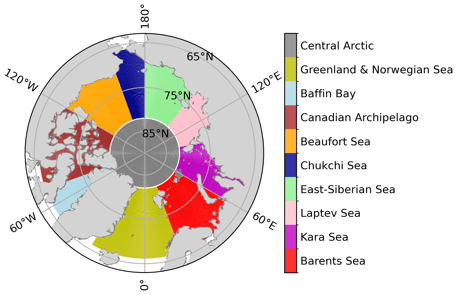
Figure 1 Map of Arctic Ocean subregions considered in this study. Lateral boundaries were defined following the oceanic region definitions by Nöthig et al. (2020) and Randelhoff et al. (2020), whereas latitudinal limits were modified and extended to uniformly cover 66–82° N for all regions except the Central Arctic (82–90° N).

2.3 Methodological challenges analysing marine biomolecules in the Arctic

Analysing ocean biomolecules in the Arctic presents specific challenges. While the REcoM simulates marine biogeochemistry beneath sea ice, under-ice production does not contribute to sea spray emissions, since ice cover prevents bubble bursting at the surface. Although sea spray emissions can occur in the marginal ice zone and within the Arctic sea ice pack from open leads and melt ponds (Leck and Bigg, 2005b; Willmes and Heinemann, 2015; Zhang et al., 2018; Rolph et al., 2020), these sources are not considered in this study. Consequently, since these sources cannot be represented, we apply a sea-ice mask that restricts the analysis to open-ocean grid cells (SIC < 10 %; Arrigo et al., 2008) exclusively for calculations of average marine parameters and aerosol OMF over the Arctic. Note that the mask does not apply to the use of the biomolecule ocean concentrations as bottom boundary condition within the ECHAM-HAM simulations. Additionally, for a more profound understanding of the particularities within the Arctic Ocean, we conducted a detailed, separate analysis of the main Arctic seas, as illustrated in Fig. 1.

In this study, Arctic trends were assessed using the non-parametric Mann–Kendall test and the Theil–Sen slope estimator. For marine variables, we must also consider that the production under ice is present. However, when computing the trends of ocean biomolecule concentration, we did not apply the ice mask described above. Excluding under-ice production led to inconsistent and unrealistic trend patterns because interannual and seasonal variability of sea ice, especially near the ice edge, strongly influences marine production. This likely reflects differing bloom dynamics in the marginal ice zone versus fully open ocean areas. Hence, we estimated the changes in the marine biomolecules by computing maximum trends of likely ice-free regions within the Arctic. To achieve this, we excluded areas overlapping the seasonal minimum sea ice concentration. This ensures that potentially open water regions, where marine organic emissions could occur over the 30 year period, are taken into account. Finally, trends of emission mass fluxes and aerosol concentration of sea salt aerosol and PMOA modelled by ECHAM-HAM are also analysed in Sect. 4.

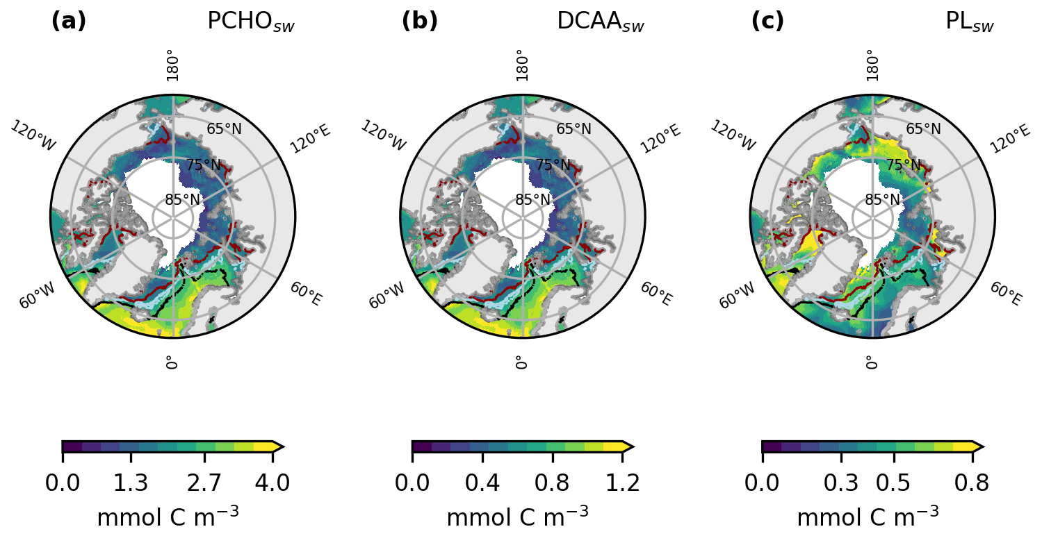
Figure 2 Maps of averaged ocean carbon concentration of (a) PCHO_sw, (b) DCAA_sw, and (c) PL_sw as a multiannual mean spanning May–September for the period 1990–2019. The black, blue and red lines depict the ice edge, defined as the contour of 10 % sea ice concentration for May, July and September, respectively.

3 Results and discussion

3.1 Geographical distribution of marine biomolecule groups

The simulated biomolecule ocean concentrations are shown in Fig. 2 as a multiannual average from May to September over the period 1990–2019. In terms of carbon contribution, PCHO_sw dominates in seawater, with a mean concentration over the Arctic circle of 1.4 mmol C m⁻³, followed by DCAA_sw (0.4 mmol C m⁻³) and PL_sw (0.3 mmol C m⁻³). The distribution of PCHO_sw and DCAA_sw (Fig. 2a and b) presents a nearly identical geographical distribution, since the latter was computed as a fraction of simulated PCHO_sw. In contrast, PL_sw spatial patterns are rather distinct (Fig. 2c). For instance, notably greater concentrations are seen in the Norwegian Sea and North Atlantic compared to the central Arctic and vice versa for the semi-labile and lipid groups, respectively. Hence, a description of the seasonal particularities of regions within the Arctic Ocean that determine the distribution of the biomolecules is provided further below.

The differing geographical distribution of the groups is determined by the production or loss mechanisms considered in the biomolecule computation. PCHO_sw represents the largest fraction of phytoplankton exuded DOC. It quickly aggregates to form TEP, which is considered a loss term in the online simulation of PCHO_sw by REcoM. This is the reason for the prominent differences in the Arctic Ocean biomolecule concentration compared to PL_sw group (see Fig. 2a).

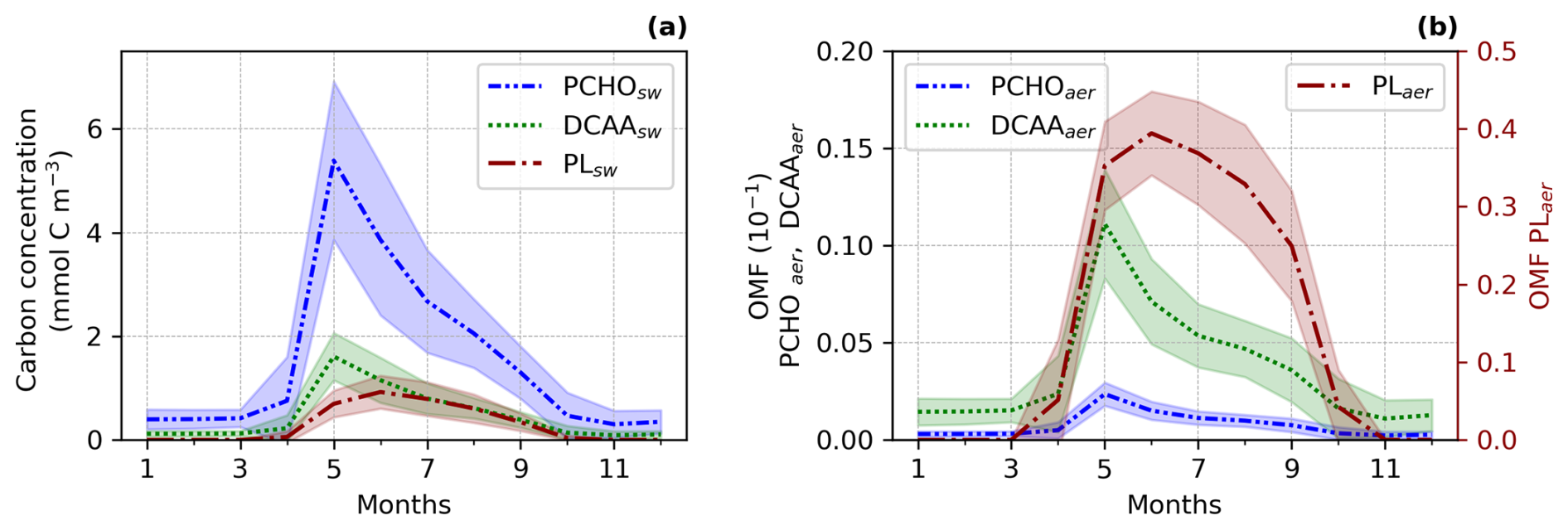
Figure 3 Seasonal climatology of (a) ocean carbon concentration for PCHO_sw, DCAA_sw and PL_sw and, (b) offline simulated organic mass fraction (OMF) in nascent aerosol from OCEANFILMS for PCHO_aer, DCAA_aer and PL_aer for the period 1990–2019 and sea ice free ocean conditions (SIC < 10 %; Arrigo et al., 2008) averaged over the Arctic. Values were over the Arctic circle (66–90° N) and the shaded area represents the spatial standard deviation of the long-term monthly mean.

3.2 Seasonality of marine biomolecule groups

The biomolecule concentrations exhibit a pronounced seasonality in the Arctic (Fig. 3). When light limitation decreases at the end of the polar night, phytoplankton bloom initiates. Figure 3a illustrates the seasonal cycle of the ocean carbon concentration of the biomolecules averaged over the Arctic Ocean from 1990 to 2019, considering solely sea ice-free ocean conditions (SIC < 10 %; Arrigo et al., 2008). The seasonal patterns vary among the organic groups. PCHO_sw and DCAA_sw ocean concentration rise sharply until May, whereas PL_sw peaks a month later. The levels of all biomolecules are high from April to October, with a gradual decline after their early-summer peak. PCHO_sw, as the major extracellular product of phytoplankton in seawater, exhibits consistently higher concentrations than DCAA_sw and PL_sw groups across months. Maximum concentration of PCHO_sw, DCAA_sw and PL_sw are 5.4 ± 1.5, 1.6 ± 0.5 and 0.9 ± 0.3 mmol C m⁻³, respectively.

The dominance of the biomolecules in the ocean during spring and summer occurs in response to the higher phytoplankton carbon concentration in the water during this period. After rapid nutrient consumption during phytoplankton growth, the bloom decays primarily due to nutrient depletion. Among the modelled phytoplankton groups, diatoms contribute to the majority of the exuded DOC in the Arctic, especially during the early stage of the bloom (Fig. B1).

The OMF in nascent aerosol shows a similar seasonal pattern, with the highest contributions in spring and summer (Fig. 3b). However, the OMF of the aerosol species (PCHO_aer, DCAA_aer and PL_aer) do not behave as their precursors in the ocean. PCHO_aer has the lowest OMF, followed by DCAA_aer and PL_aer. The high surface affinity of lipids positions PL_aer as the major contributor to marine organic aerosol during months with high biological productivity. Values are as high as 0.4 ± 0.05. OMF for PL_aer is at least one to two orders of magnitude higher than for PCHO_aer and DCAA_aer, respectively. Whereas PCHO_aer and DCAA_aer remain within 10⁻³ and 10⁻² throughout the year (note that PCHO_sw has the lowest surface affinity), PL_aer decreases to negligible values as the PL_sw concentration in the ocean approaches almost zero in winter months (Fig. B1).

Note that we averaged the ocean concentrations over the whole Arctic region, which does not represent the spatial particularities and seasonality of subregions within the Arctic circle (Fig. 2). Ocean marine productivity in REcoM is limited by either light or nutrient availability, which is influenced by physical factors such as advection, mixing, stratification, sea ice, and ocean temperature (Schourup-Kristensen et al., 2018). Hence, biomolecule concentrations and OMF exhibit different patterns across Arctic sites, with pronounced variation among regions from May to August (see Fig. B2a, b, and d).

Sea ice is a controlling factor in the initiation of the bloom (Ardyna and Arrigo, 2020), as well as the magnitude of the biomolecule production. For instance, in the Central Arctic, where light is the most limiting factor (Schourup-Kristensen et al., 2018) with sea ice only partially retreating by mid-summer alongside low nutrient availability, a less prominent late bloom shifts the initiation of phytoplankton carbon release to May (see Fig. B2b and c). Conversely, the Greenland, Norwegian, and Barents Seas have the lowest sea ice coverage among Arctic subregions (see Fig. B2e) and lower phytoplankton carbon concentrations (see Fig. B2c). These seas are also strongly influenced by the lateral transport of nutrients from the North Atlantic Ocean (Harrison et al., 2013). Other regions such as the Chukchi Sea, the Russian shelf, the Beaufort Sea and the Canadian Archipelago are seasonally sea ice covered (Fig. B2e). In the coastal zones of these regions, sea ice cracks and melts, which, along with local factors, rapidly trigger marine primary production. In addition, the Eastern Siberian, Southern Beaufort, Laptev, and Kara Seas are characterised by a strong land influence, and higher concentrations of biomolecules are attributed to riverine nutrient supplies (Miquel, 2001; Wang et al., 2005; Karlsson et al., 2011; Oziel et al., 2025). Moreover, ice-edge blooms and high nutrients near shore in ice-free conditions are the sites with the highest PL_sw production (Fig. 2c), suggesting that its spatial distribution is highly sensitive to sea ice dynamics.

Lastly, we analyse the yearly seasonality in Arctic subregions to examine how the initiation and duration of biomolecule production have changed over the 30 year period. While the seasonal patterns remained stable for the Canadian Archipelago, Baffin Bay and, Barents, Greenland and Norwegian Seas, a pronounced interannual variability occurs for the inner Arctic seas. Among these, the Beaufort and Kara seas show strong indications that biomolecule release initiates 1 month earlier during the second half of the study period compared to 1990–2004 (see Fig. C1). Other studies based on satellite products have found trends in phytoplankton blooms shifting towards an earlier maxima (Kahru et al., 2011; Zhao et al., 2022). Similarly, recent modelling analysis by Manizza et al. (2023) also points towards earlier spring blooms in the inner Arctic seas.

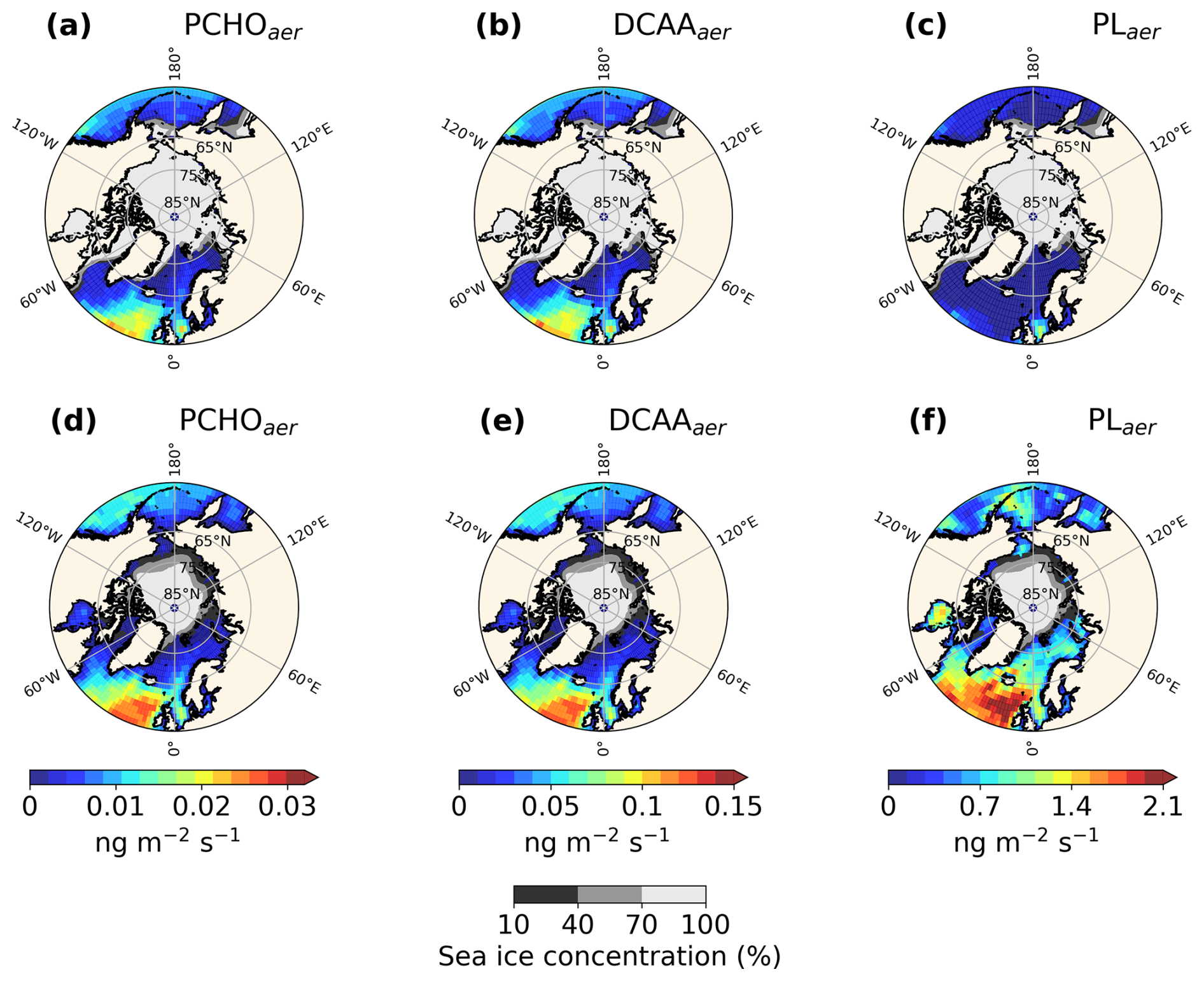
Figure 4 Maps of Surface emission mass flux of (a, d) PCHO_aer, (b, e) DCAA_aer and (c, f) PL_aer for the Arctic averaged over (a–c) January–February–March and (d–f) July–August–September for the simulated period 1990–2019.

3.3 Patterns of PMOA emissions

Like the biomolecule concentration in the ocean, PMOA emission mass flux also follows a specific seasonality in the Arctic (Fig. 4). Sea ice strongly influences marine aerosols by affecting ocean bioactivity and limiting sea spray emissions via bubble bursting. As a result, marine aerosol emission mass fluxes are expected to increase as sea ice melts. In the next sections, we present the geographical distribution of the emissions as well as their seasonality in contrast to the main emission drivers.

3.3.1 Geographic distribution

Figure 4 shows the geographical distribution of mean emission flux for each group for the winter months January–February–March and summer July–August–September. During the polar night, biomolecules in the Arctic Ocean remain very low (Fig. 3a–c). Hence, weak emission fluxes are reported in winter with a total PMOA flux of 1.4 × 10⁻³ $\mathrm{ng}{\mathrm{m}}^{-\mathrm{2}}{\mathrm{s}}^{-\mathrm{1}}$. The minimum in marine emissions in winter is accompanied by the maximum sea ice concentration for the season. Marine aerosols are confined to the North Atlantic and Pacific oceans, where high winds promote elevated sea spray emissions. Nonetheless, PCHO_aer and DCAA_aer (Fig. 4a and b) still contribute over the southern Arctic waters (Greenland and Norwegian Seas), with emissions as high as 0.04 $\mathrm{ng}{\mathrm{m}}^{-\mathrm{2}}{\mathrm{s}}^{-\mathrm{1}}$. On the other hand, PL_aer average flux (Fig. 4c) is negligible for this period (2.2 × 10⁻⁶ $\mathrm{ng}{\mathrm{m}}^{-\mathrm{2}}{\mathrm{s}}^{-\mathrm{1}}$) whereas the other two groups dominate. The mean values for PCHO_aer and DCAA_aer are 2.5 × 10⁻⁴ and 1.2 × 10⁻³ $\mathrm{ng}{\mathrm{m}}^{-\mathrm{2}}{\mathrm{s}}^{-\mathrm{1}}$, respectively.

In contrast to winter, summer fluxes are moderate for the North Atlantic and Pacific Oceans (Fig. 4d–f). Nevertheless, mean quantities are greater over the Arctic compared to winter months with values of 7.1 × 10⁻⁴, 3.4 × 10⁻³ and 1.8 × 10⁻¹ $\mathrm{ng}{\mathrm{m}}^{-\mathrm{2}}{\mathrm{s}}^{-\mathrm{1}}$ for PCHO_aer, DCAA_aer and PL_aer, respectively. As the phytoplankton bloom sets in during the melting season, marine organic aerosols become relevant and expand northward over the Norwegian, Greenland, Baltic, and Chukchi Seas. Unlike winter, the minimum in sea ice for the period leads to a maximum in organic emissions (0.18 $\mathrm{ng}{\mathrm{m}}^{-\mathrm{2}}{\mathrm{s}}^{-\mathrm{1}}$). Among the aerosol groups, PL_aer contributes to most of the organic mass fraction in aerosols. Compared to the other groups, the contribution of PL_aer is widely spread across the Arctic seas, being the species with the strongest increase from winter to summer. Note that the marine aerosol contribution varies per species and regions within the Arctic circle (Fig. 4). A comprehensive analysis of the seasonal characteristics of marine emissions is presented further below.

To study how total marine emissions in the Arctic have changed over time, we calculated the average of the total fluxes and burden of marine aerosols for the first and second half of the simulated period (Table 1). For every year, the values were obtained by aggregating the daily results from all grid cells within the region, and the resulting annual totals were averaged for the first and second 15 years of the 30 year simulation. As expected, PL_aer accounts for the majority of PMOA and represents 2.4 % of total emitted SS for the 30 year period. Conversely, PCHO_aer and DCAA_aer make up to 0.07 % and 0.02 %, respectively. Note that SS emissions include the accumulation and coarse modes as a model output variable, while PMOA is emitted in the accumulation mode only. Hence, the actual PMOA/SS fraction may be higher if we consider the accumulation mode only.

Table 1 Total emission flux, atmospheric burden, and deposition of marine aerosol particles calculated by summing daily values across all Arctic grid cells and averaging yearly totals over two 15 year periods and the full 30 year period in bold.

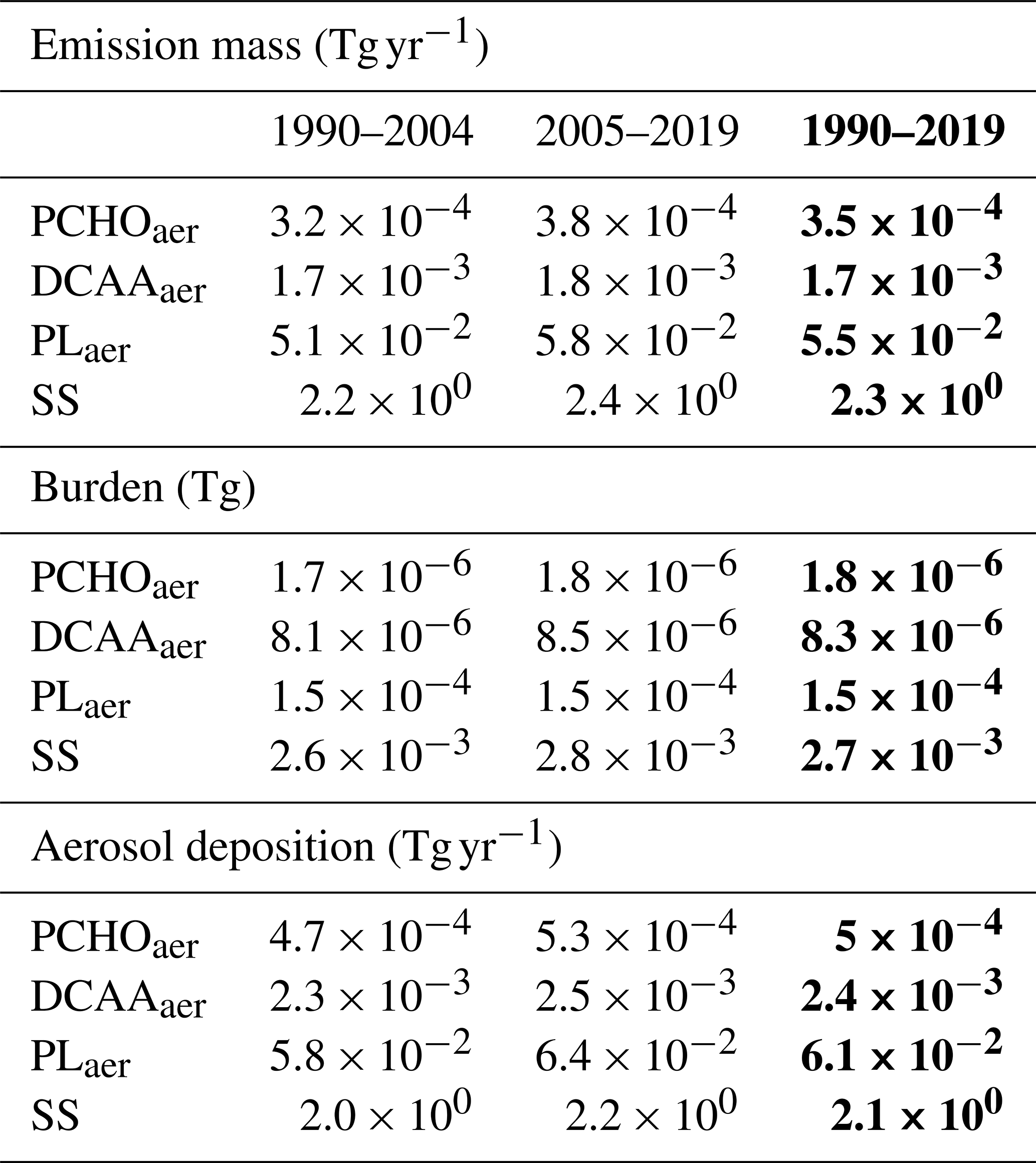
For the 15 year periods, a noticeable increment in the emissions is seen for all species (Table 1). PCHO_aer presents the largest augment, with an 19.3 % increase from 1990–2004 to 2005–2019. Conversely, DCAA_aer, PL_aer, and SS growth is less strong, with values of 12 %, 13.9 % and 10.6 %, respectively. In our model, burden values also rise, although not as significant as the changes in emissions. For PCHO_aer, the positive variations in the burden are also high (6.8 %) in contrast to a lower increase in DCAA_aer and PL_aer (4.5 % and 4.2 %). This indicates that an increment in aerosol sources will have a positive impact on the column burden. Similarly, the aerosol removal increases accordingly (Table 1). Wet deposition in stratiform clouds and in-cloud processes are the main processes that govern the loss of marine organics. For PCHO_aer, DCAA_aer and PL_aer, the percentage of increase is about twice larger than for the burden (13.9 %, 8.9 % and 9.7 %, respectively). In contrast, the change in SS loss from the first half to the second half of the period is only slightly larger than the burden increase (8.8 %). Hence, estimated PMOA residence time in the atmosphere shortened for all species from 4 % to 6 %. The noticeable differences between PL_aer, DCAA_aer, and PCHO_aer are primarily attributed to the variations in the geographical distribution (Fig. 4) and seasonality of aerosol fluxes (see next section) in the Arctic.

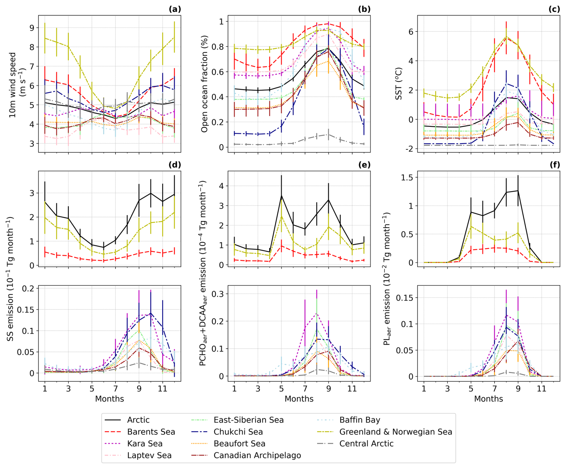
Figure 5 Seasonal climatology of (a) 10 m Wind speed, (b) Open ocean fraction, (c) SST and emission fluxes of (d) SS, (e) PCHO_aer + DCAA_aer and (f) PL_aer for the period 1990–2019 simulated by ECHAM-HAM model averaged over the Arctic and all seas within the Arctic Ocean (Fig. 1). Monthly emissions were obtained by summing the daily values across all grid cells in the region and then averaging over the 30 year period. The error bars indicate the multiannual standard deviation. Subregions with small emission fluxes are shown in a separate panel for better representation.

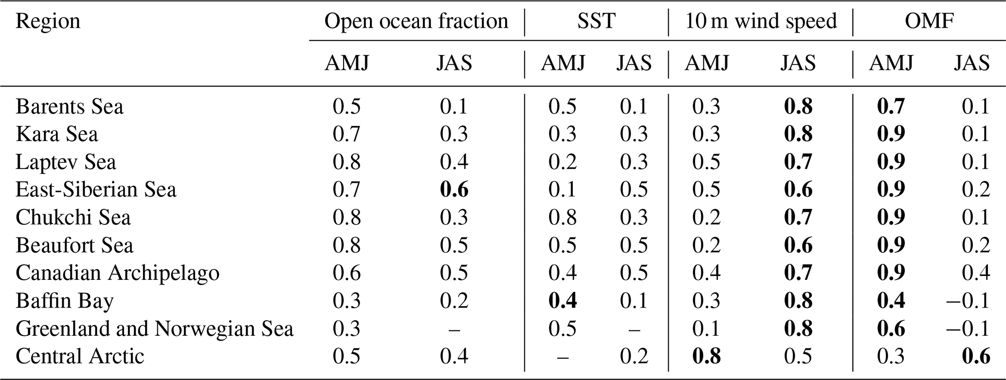
Table 2 Spearman correlation coefficients between daily total PMOA emission flux and emission drivers for the Arctic subregions over April–May–June (AMJ) and July–August–September (JAS). Only statistically significant cases (p-value < 0.05) are shown. The absolute maximum values per region are highlighted in bold.

3.3.2 Seasonality of sea spray aerosol and emission drivers

Wind is the primary driver of SS and PMOA emission fluxes. This is followed by a linear relationship between the open ocean fraction and a correction factor based on SST (Sofiev et al., 2011). Additionally, PMOA depends on marine productivity, as reflected in OMF levels. The relevance of these drivers may vary across Arctic subregions. To disentangle the relative influence of sea spray emission drivers in the ECHAM-HAM model, in this section, we discuss the seasonality of SIC, SST and 10 m wind speed in relation to sea salt fluxes and their impact on the PMOA emissions in the Arctic (Fig. 5). In addition, the correlation of total PMOA emissions with each emission driver is summarised in Table 2 for all Arctic subregions.

Figure 5a shows the average 10 m winds for the Arctic subregions. In the neighbouring waters of the North Atlantic Ocean, the Baffin Bay, the Barents and Chukchi seas, winds follow the seasonal meteorological conditions, with intensified velocities in the winter months. For the inner Arctic seas, patterns are more heterogeneous. The Central Arctic, Kara Sea, Beaufort Sea and Canadian Archipelago do not present a pronounced seasonality, whereas the Laptev and East-Siberian winds tend to be higher in summer.

Open ocean fraction follows a similar seasonality for all Arctic subregions, as sea ice shrinks through the summer and refreezes during winter (Fig. 5b). Before the onset of the melting season, the Greenland and Norwegian Seas have the highest open water fractions, approaching 80 %. The Barents Sea ranks next, with values between 60 % and 70 %. In contrast, the Central Arctic experiences only a modest summer SIC reduction, maintaining an open water fraction generally below 10 % throughout the year. All other subregions show a sea-ice reduction of about 40 %, which is most pronounced in September, with the Beaufort Sea, Canadian Archipelago, East Siberian Sea, and Chukchi Sea exhibiting the strongest transformations.

Lastly, the Arctic's rising SST (Fig. 5c) corresponds to the increase in the fraction of open ocean. The amplitude of SST for each region varies between one and two degrees Celsius and is similar to that seen in Fig. 5b. Nevertheless, for the Chukchi Sea, seasonality is more pronounced given the strong changes in SIC. Similarly, the Greenland, Norwegian, and Barents seas show strong seasonal patterns; however, temperatures are warmer and remain positive throughout the year. Overall, SST ranges between −2 to 6 °C. Within this temperature range, the Sofiev et al. (2011) SST correction factor used in the SS model representation remains relatively constant for particles in the accumulation mode, the only size class contributing to PMOA emissions. Therefore, in this case, SST has a lesser effect on marine organic emissions. Nonetheless, ocean temperatures modulate hydrographic conditions, strongly affecting marine productivity and, in turn, PMOA emissions.

Sea salt aerosol seasonality shows very similar patterns to the 10 m wind speed for the Barents and especially the Greenland and Norwegian Seas, in which the emissions are the largest in the Arctic Ocean (Fig. 5d). Values steadily decrease from January to June, then increase smoothly until October. In contrast, given the cyclic life of phytoplankton blooms, ocean biomolecules and OMF increase during the polar day and sharply decay at the end of the Arctic summer. Consequently, organic aerosol emission fluxes present distinct characteristics compared to SS and among Arctic subregions (Fig. 5e and f). Furthermore, the interannual variability of PMOA groups is stronger during the high-productivity season, whereas SS deviations are larger during winter. The most relevant discrepancies with SS seasonal patterns are seen in the Barents, Greenland and Norwegian Seas, in which the curve slightly resembles the biomolecule OMF instead (see also Fig. 3d and e). Nonetheless, due to stronger SS fluxes, the magnitude of organic aerosol emissions remains larger in the Nordic Seas than in other Arctic subregions. Conversely, in the Central Arctic, all marine aerosol fluxes are extremely low despite stronger-than-Arctic-average winds, despite the smallest open ocean areas for sea spray occurrence.

Marine organic species present different seasonality and abundance in the ocean and atmosphere (see also Fig. 3b). For instance, PL_aer has notable contributions during the Arctic summer, whereas the semi-labile compounds also contribute outside the bloom period (see also Fig. 4a and b). Note that PCHO_aer + DCAA_aer emissions have a bimodal distribution for the Nordic seas, with a global maximum in May. In these areas, contributions drop to their minimum in July, when wind velocities are lowest, and then rise to a second maximum in September, as winds intensify. This peak later in summer is less prominent in the Barents Sea compared to the Norwegian and Greenland Seas. Values continue to decay until November, with a moderate increase during the polar night, a period in which PL_aer production is absent. Figure 5f shows that the PL_aer emission fluxes have a similar pattern to that of PCHO_aer + DCAA_aer for the Greenland and Norwegian Seas. Interestingly, in the Barents Sea, PL_aer does not have a bimodal pattern and remains high from May to June, corresponding to the PL_aer OMF.

Notably, lower emissions of marine biomolecules occur in the other Arctic subregions due to lower sea salt fluxes. As sea spray occurrence is strongly affected by sea ice cover, organic aerosols become more relevant towards the end of the melting season. Hence, organic emissions peak from July to September and decline to values near zero throughout the winter. For these regions, PL emission seasonality has more similarities to that of PCHO_aer + DCAA_aer. Nevertheless, the latter often reach their seasonal peak ahead of PL_aer. The Kara Sea has the highest emissions, followed by the East Siberian Sea, the Chukchi Sea, and the Laptev Sea. The summer sea-ice melt likely drives the difference in emissions magnitude among these seas. Note that, compared to sea salt, the slopes and the smoothness of the curves vary for all marine species. Moreover, regions with the highest SS fluxes are not necessarily those with the highest organic emissions. For instance, in contrast to organic species, SS contributions in the Chukchi Sea are comparable to those in the Kara Sea Fig. 5d). These distinguishable characteristics evidence the effect of marine biological activity on emission seasonality patterns.

Analysis of the annual seasonality of PMOA emissions did not reveal a clear shift toward earlier onset. In the Beaufort Sea, emissions show a tendency to occur approximately 1 month earlier during the second half of the study period; however, the patterns are weak and not sufficiently robust to draw conclusions (not shown).

In summary, modelled marine emission patterns in the Arctic result from a combination of four main controlling factors: surface winds, open-ocean grid-cell fraction, SST, and marine productivity (with OMF, as a proxy for marine biomolecule contribution). The strong power-law dependency of SS on wind speed (Long et al., 2011) produces significantly higher values for slightly stronger winds (e.g., North Atlantic Ocean in contrast to the Baltic Sea in Fig. 5a and d), dominating PMOA emissions. Nonetheless, emission drivers could have differing seasonal effects on emissions. To assess the differences in the Spearman correlation between daily total PMOA emissions and their drivers, Table 2 summarises the correlation coefficients computed for spring (April–May–June) and summer (July–August–September) across Arctic subregions. As marine productivity rapidly increases when the phytoplankton bloom sets in (see Fig. 3), emissions are strongly correlated to OMF in spring. In addition, the open ocean fraction generally shows moderate to high coefficient values. Conversely, 10 m wind speed shows the highest correlations with the emissions during summer. Nevertheless, the open ocean fraction remains an essential modulator in the East Siberian, Laptev, and Beaufort seas. At the same time, SST and OMF typically exhibit moderate or low correlations with emissions. As OMF declines after May or June (see Fig. B2d), this emission driver exerts a weaker influence on emissions thereafter. In the Central Arctic, the late biomolecule production shifts the OMF peak to August, explaining the stronger summer correlation than spring.

4 Arctic trends

4.1 Impact of sea ice retreat on PMOA precursors

To gain deeper insights into how marine biomolecules and their organic contributions to aerosols have evolved under the current Arctic warming, this section discusses observed trends in the Arctic. Figure 6 shows the trends of the average ocean concentration of PCHO_sw and PL_sw over July–August–September (summer) in the Arctic region. Given that the trends of the semi-labile groups present similar characteristics, DCAA_sw concentration is not included in Fig. 6 but shown in Fig. D1. The trends of SIC and the net primary production modelled in FESOM-REcoM are also included. To restrict our analysis to potentially ice-free regions where marine emissions may occur, we overlaid the seasonal minimum SIC on trends of ocean organic quantities, thereby visually excluding areas that are likely permanently ice-covered. The trends for the months April–May–June (spring) are included in the supplement in Fig. H1. PCHO_sw concentration (Fig. 6a) increases for most Arctic subregions. The maximum absolute trends exceed 0.04 $\mathrm{mmol}\mathrm{C}{\mathrm{m}}^{-\mathrm{3}}{\mathrm{yr}}^{-\mathrm{1}}$ in the Canadian Archipelago, East-Siberian and Laptev seas (Fig. E1). DCAA_sw trends remained smaller, only reaching up to 0.01 $\mathrm{mmol}\mathrm{C}{\mathrm{m}}^{-\mathrm{3}}{\mathrm{yr}}^{-\mathrm{1}}$ (see Figs. D1 and E1). For most subregions, and especially the eastern Arctic, trends are consistently increasing. PL_sw concentration (Fig. 6b), on the other hand, increases on the Russian shelf and in the Beaufort Sea by up to 0.02 $\mathrm{mmol}\mathrm{C}{\mathrm{m}}^{-\mathrm{3}}{\mathrm{yr}}^{-\mathrm{1}}$ (see also Fig. E1), while in the Baffin Bay, Canadian Archipelago and Nordic Seas, concentrations decreased (−0.01 $\mathrm{mmol}\mathrm{C}{\mathrm{m}}^{-\mathrm{3}}{\mathrm{yr}}^{-\mathrm{1}}$).

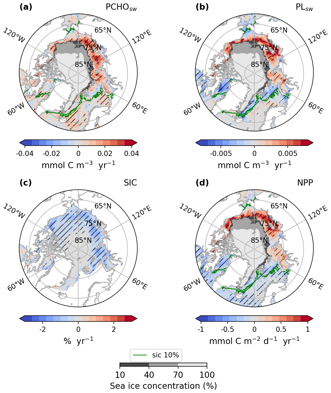
Figure 6 Arctic trends of (a) PCHO_sw and (b) PL_sw ocean concentration, (c) sea ice concentration and (d) net primary production from FESOM-REcoM model for July–August–September of the simulated period 1990–2019. The hatching indicates the areas over which trends are significant (Mann–Kendall test, p-value < 0.05). The green contour line depicts the average season 10 % sea ice concentration. The minimum seasonal SIC for the period occurred in September 2012, and it is also represented in shaded grey.

In summary, the trends show regional differences across biomolecule groups. For PL_sw, the largest density of model grid points with statistically significant trend is found in regions with minor sea ice changes (Baffin Bay, Barents, and Greenland and Norwegian Seas in Fig. 6a and b). Conversely, for PCHO_sw and DCAA_sw, this is more prominent in the inner Arctic seas, with the most relevant positive changes observed in the Russian shelf. PL_sw has decreased in some regions, such as the Canadian Archipelago and Baffin Bay, with pronounced variations. Although the increasing trends, when present, are generally stronger than the negative changes. Note that regions with a strong decline in sea ice generally have a noticeable and statistically significant increase in marine primary production (see Fig. 6c and d). As a result, biomolecule concentrations consistently increase in the eastern Arctic subregions during summer.

On the other hand, the extent of sea ice cover masks the marine biomolecules that potentially contribute to aerosols during spring (Fig. H1). Hence, in the Russian shelf, the trend is absent for all marine organic groups. Nonetheless, a strong increase in ocean carbon concentration occurs in Baffin Bay, the Canadian Archipelago, and the Nordic seas for PCHO_sw and DCAA_sw, largely exceeding summer values (see Fig. H2). Lastly, PL_sw decreasing trend also persists in the Nordic Seas; however, somewhat weaker and stronger than in summer for the Barents and Greenland seas, respectively.

Overall, the geographical distribution of PL_sw trend has similar characteristics to the NPP changes, especially in the inner Arctic and towards the sea ice edges (Figs. 6b, d and H1b, d). This close agreement is expected, as PL_sw is a direct product of phytoplankton carbon exudation. Nevertheless, in the Southern Norwegian and Barents seas during summer, south of the sea ice edge, PL_sw showed a slightly positive or nearly absent trend that could be caused by depleted DIN. Under this condition, the carbon-overflow hypothesis (Engel et al., 2004, 2020) could explain the higher phytoplankton exudation rates. Similarly, for the semi-labile groups, this applies to multiple regions. However, the trend for the majority of the Arctic subregions predominantly increases, in contrast to the negative trend seen in NPP and PL_sw. The discrepancies are explained by the formation of TEP, which shows closer patterns to the NPP, as they rapidly form after PCHO_sw exudation and represent a loss to the biomolecule. Interestingly, this process is more evident in sea ice-free regions.

The FESOM-REcoM modelled NPP trends presented here have similar geographic patterns to the yearly changes discussed by Arrigo and van Dijken (2015) and Lewis et al. (2020) for most Arctic seas. A NPP increase in the inner Arctic waters, and only little variations or a slight decline in the Nordic seas and Arctic outflow regions have been reported in satellite-based analysis for the period 1998–2012 by Arrigo and van Dijken (2015). Moreover, Cherkasheva et al. (2025) confirmed for the Greenland Sea that no significant NPP trend is observed for the 1998–2022 time series, consistent with the minimal changes we find in this region. However, some discrepancies are visible in the Barents and Chukchi Seas when comparing the results in Arrigo and van Dijken (2015) to those presented here. Besides the extended range of years we simulated in our study, another driving difference is the separation of seasons considered in the analysis. For instance, our simulations extend beyond the 2012 and for the late summer months (July–August–September), which is usually the time by which nutrients are at their lowest in Arctic waters (see DIN concentration in (Schourup-Kristensen et al., 2014)), potentially leading to the discrepancies seen in the Barents Sea compared to Arrigo and van Dijken (2015) and Lewis et al. (2020). Lastly, the trends calculated in the Chukchi Sea might not be representative of the region, given the limited area in which the trends are significant.

As stated in Leon-Marcos et al. (2025), note that the computation of the biomolecules does not consider ocean temperature effects on phytoplankton exudation (Zlotnik and Dubinsky, 1989; Guo et al., 2022). Nevertheless, a mesocosms study by Engel et al. (2011) demonstrated that for polar waters, an increase in seawater temperature (from 0 to 6 °C) leads to a faster production and larger accumulation of dissolved combined carbohydrates (analogous to PCHO_sw) with no impact on the dissolved amino acids (proxy for DCAA_sw). This could be relevant in the current Arctic warming conditions with SST anomalies of several degrees Celsius in summer (Steele et al., 2008) that continue to exist in future Arctic projections.

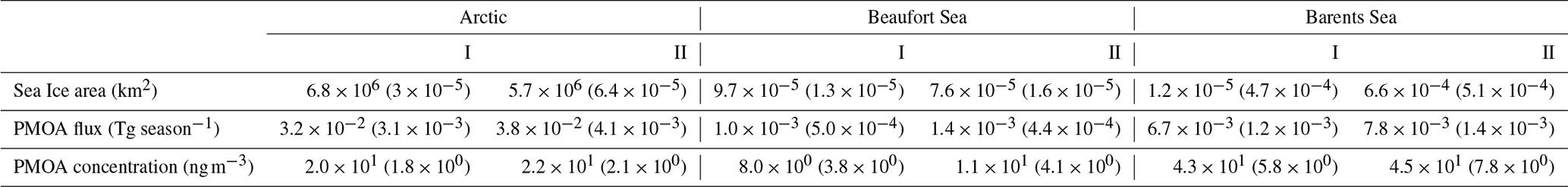
Table 3 Values of sea ice area, total emission mass flux and near-surface average PMOA concentration over the Arctic and Arctic subregions Beaufort Sea and Barents Sea analysed in Fig. 7 for 15 year periods, 1990–2004 (I) and 2005–2019 (II) for July–August–September. Seasonal emission totals are derived by adding daily values throughout the season across all grid cells in the region. The standard deviation of the multi-year average is shown in parentheses.

4.2 Historical and present trends in the PMOA emissions

Here, the pan-Arctic trends in sea ice extent, SST and PMOA emission anomalies are investigated. Figure 7 shows the time series of averaged summer sea ice area and total PMOA emission anomalies with respect to the period mean for 1990–2019 simulated by the ECHAM-HAM model. The yearly mean values for the Arctic Ocean and preferred subregions within the Arctic Circle are considered. SST is included as an additional panel for better representation. Among all subregions, the ones presented here are the only cases for which sea ice area, SST, and PMOA anomalies showed significant trends over the 30 year period. Sen's slope value and intercept are always included. To better illustrate changes in absolute aerosol levels, Table 3 displays the 15 year averages of PMOA flux, concentration, and sea ice area.

Figure 7 Time series of sea ice area in blue, averaged PMOA (PCHO_aer + DCAA_aer + PL_aer) emission mass flux anomalies in red and mean SST as an additional panel in grey for (a) the Arctic, (b) Beaufort Sea and (c) Barents Sea as defined in Fig. 1 for July–August–September of the simulated period 1990–2019 by ECHAM-HAM model. Dashed lines depict the trend line calculated using the slope and intercept values derived from the Theil–Sen slope estimator.

The sea ice area for the Arctic Ocean has suffered a critical decline after 2005 (Fig. 7a). A decreasing trend is visible throughout the period. This behaviour is obvious when comparing the extreme values. The maximum summer sea ice extent occurred in the first half of the period in 1996 with 7.4 × 10⁻⁶ km² in contrast to a minimum of nearly half 4.6 × 10⁻⁶ km² in 2012. Conversely, PMOA flux anomalies show an opposite trend to sea ice changes (Fig. 7a). Note that after 2005, positive anomalies are more frequent and stronger. Values were as low as −5.1 × 10⁻⁶Tg season⁻¹ in 2001 and went up to 5.1 × 10⁻⁶Tg season⁻¹ in 2005. In contrast to the minimum sea ice area, the peak in positive anomalies occurs earlier. Moreover, the changes in both variables between periods are not proportional. While other emission drivers could modulate PMOA emissions, in the Arctic, only sea ice extent and SST showed significant trends over the study period. Like PMOA anomalies, SST have increased since 1990, rising by about 1 °C. While during 2007–2019, SST steadily rose to 2 °C, values generally remained below 1 °C for the first half of the period. Overall, a moderated response of the fluxes to the sea ice retreat and SST increase is evident in Fig. 7a. This was also presented in Table 2 as the correlation between the emission anomalies and variables controlling the emissions.

To illustrate the strong spatial variability and regional heterogeneity in the Arctic Ocean, the time series of the Beaufort and Barents Seas are presented as examples. The decline in sea ice area and the increase in marine emission anomalies are especially pronounced in the last decade of the study period (see Fig. 7b and c). The minimum sea ice extent in the Beaufort Sea was reached in 2012 with 5 × 10⁻⁷ km². In the Barents Sea, values are significantly lower compared to inner Arctic seas and drop to 7.7 × 10⁻⁹ km² between 2018 and 2019. In these subregions, positive marine emission anomalies occur more frequently during the second half of the period than in 1990–2004. Although the decline in Arctic sea ice area is stronger than in individual subregions, trends in marine emission anomalies remain similar across all cases. Figure 7b and c illustrate the link between the fraction of open ocean and marine emissions. In most years, a larger sea ice area corresponds to lower marine aerosol anomalies, whereas a smaller ice cover corresponds to higher fluxes. From the first to the second half of the period, average temperatures rose about 1 and 1.5 °C in the Beaufort Sea and Barents Sea, respectively. Importantly, emissions are largely regulated by sea ice area and SST for the Beaufort Sea, while the correlation is moderate for the Barents Sea (see Table 2). In the latter case, surface winds strongly drive the emissions.

For the Beaufort Sea, the magnitude of the emission anomalies is comparable with the Arctic mean (Fig. 7b). The largest positive and negative anomalies occurred in 2008 (6.1 × 10⁻⁶ Tg yr⁻¹) and 1991 (−5.1 × 10⁻⁶ Tg yr⁻¹). On the other hand, anomalies are stronger for the Barents Sea, given the larger fraction of open ocean (Fig. 7c). A prominent peak is seen in the last year of the study period, with a value of 2.3 × 10⁻⁵ Tg yr⁻¹. For this region, sea ice cover has a weaker effect on marine aerosol occurrence.

To examine the changes in other aerosol quantities, Table 3 summarises the total emission fluxes and near-surface average concentration in addition to sea ice over both halves of the simulated period. With this, we revealed the correlation between sea ice retreat and marine aerosol quantities. An increase of 17.3 % was attributed to the Arctic PMOA emissions from 1990–2004 to 2005–2019, in contrast to a 16.5 % reduction in summer sea ice area. Similarly, PMOA concentration also grew by 7.7 %. The rate of mean sea ice reduction in the Barents Sea from the early to the late fifteen years is the most notable. The decline is twice larger than that in the Beaufort Sea, with about 22 % and 42 % decrease, respectively. The latter presents the most drastic increment in the emissions and aerosol concentration, rising more than 30 % and 40 %, respectively. However, fluxes in the Barents Sea experienced slightly more than half the increase detected in the inner Arctic sea, while aerosol concentration only rose by 4.5 %.

In spring, seasonal mean aerosol emission fluxes and PMOA concentrations across the Arctic are lower than in summer (Table F1), while sea ice cover is clearly broader. Although the decline in spring sea ice area is weaker than in summer, it remains detectable. Consequently, increases in aerosol emission fluxes during spring are less pronounced than in the warm season. PMOA concentration tends to decline in the second half of the modelled period. On the other hand, in the Beaufort Sea, the PMOA concentration increase during spring is less pronounced than that of summer. This might be related to the steep sea ice loss in summer, with over 20 % reduction in the last fifteen years compared to only 3.1 % negative change through April–May–June. Lastly, for the Barents Sea, the variation in aerosol quantities is stronger for the early melting season despite the less variable sea ice area, but a slightly stronger SS emissions change rate.

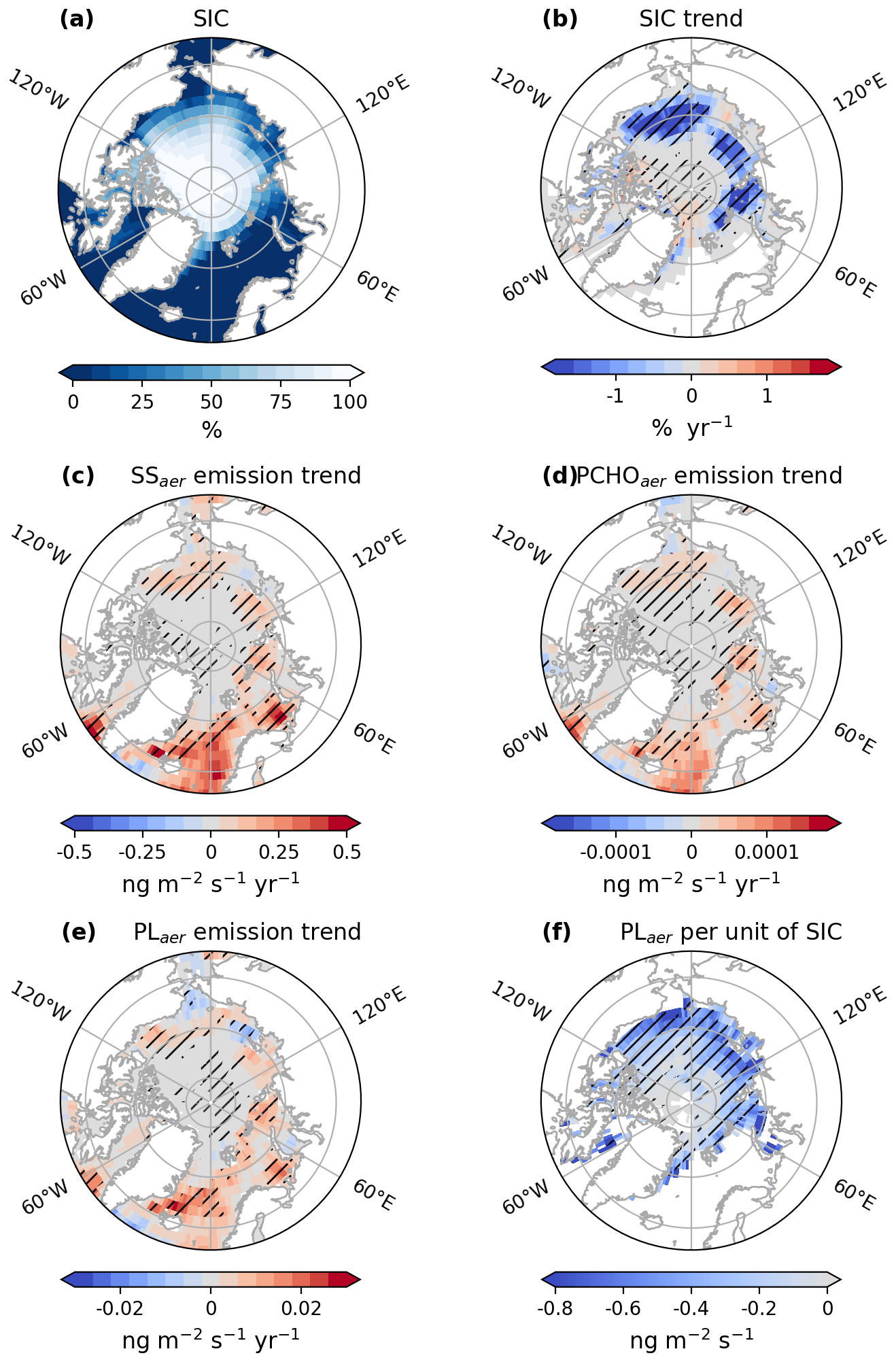
Figure 8 Maps of (a) average sea ice concentration (SIC), (b) trend of SIC, trends of emission fluxes of (c) SS, (d) PCHO_aer, (e) PL_aer and (f) changes of emission fluxes of PL_aer per unit of SIC for SIC > 20 %, for July–August–September of the simulated period 1990–2019 by ECHAM-HAM model. The trend of PL_aer per unit of sea ice was computed based on a linear regression model. The hatching indicates the areas over which trends are significant (Mann–Kendall test or t-test, p-value < 0.05).

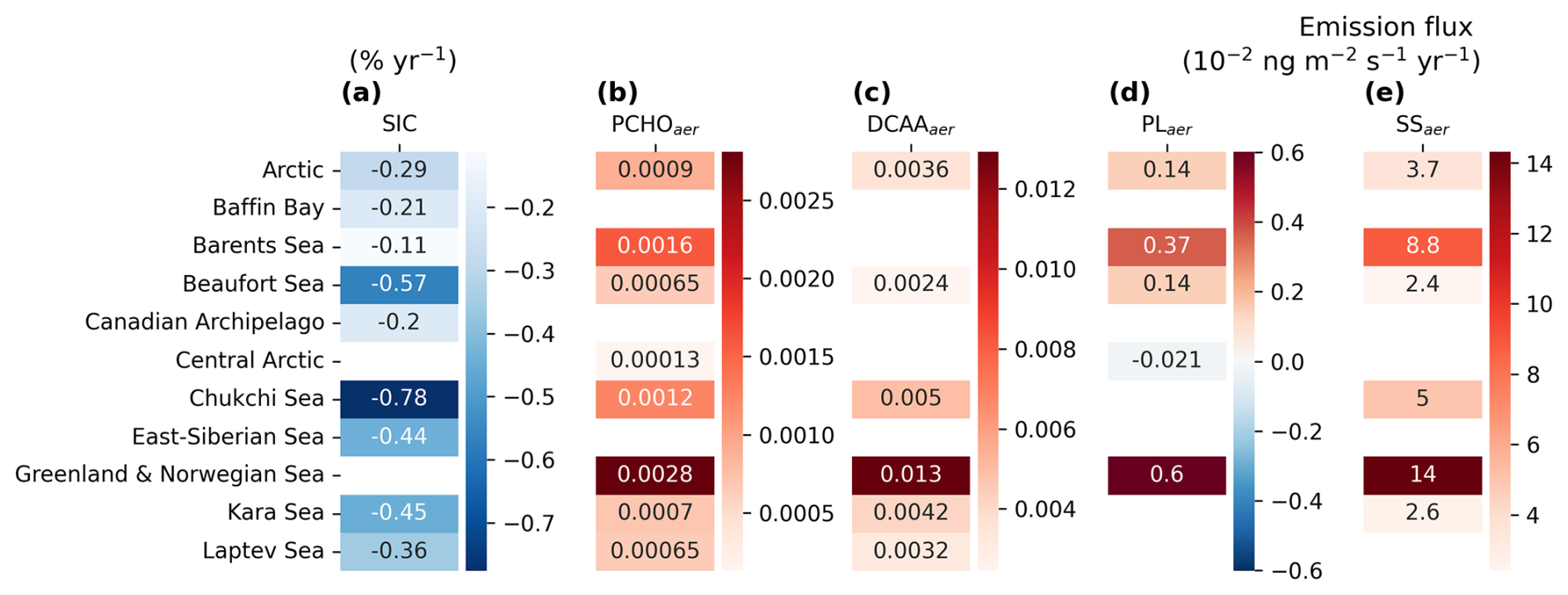
Figure 9 Heatmaps of trends over the Arctic and subregions defined in Fig. 1 for averaged (a) SIC, aerosol emission mass flux of (b) PCHO_aer, (c) DCAA_aer, (d) PL_aer, and (e) SS simulated by ECHAM–HAM model for July–August–September of the period 1990–2019. Only regions where the trend was significant are included (Mann–Kendall test, p-value < 0.05).

4.3 Regional changes in PMOA emissions and budget

As the analysis shows, there is no uniform pan-Arctic trend in the emissions and occurrence of PMOA. Figure 8 illustrates the sea ice concentration in ECHAM-HAM simulations (from AMIP) and the regional trends of SIC and PL_aer, PCHO_aer and SS emission flux across the Arctic as computed with ECHAM-HAM (see also DCAA_aer in Fig. D2). The changes per unit of SIC of PL_aer emission mass fluxes are also presented. Additionally, Fig. 9 shows the trends of marine aerosol fluxes per region within the Arctic circle. Due to the high variability of surface winds, the 10 m Wind velocity trend has overall low significance in the Arctic (see Fig. G1) and therefore is not included in Fig. 9.

The strongest sea ice concentration variations occurred at the outer edges of the ice pack (for SIC < 80 % in Fig. 8a). A significant loss in sea ice is evident for most areas in the Arctic (Fig. 8b). The strongest decrease occurs in the Chukchi and Beaufort Seas (see Fig. 9a). Nonetheless, for all regions, a decline of SIC predominates. Nonetheless, a few regions, such as the northern Canadian Archipelago and the north coast of Greenland, exhibit areas with a slight, statistically significant positive trend.

The increase in aerosol emission fluxes in the Arctic is attributable to larger areas of open ocean water fraction (Fig. 8c–e). The strongest changes in PMOA and SS emission mass fluxes are seen in the Southern Barents Sea and in the Greenland and Norwegian Seas (see Fig. 8c). Surface wind speeds are also determinant, especially in regions with reduced SIC (Fig. G1). Moreover, a decrease in emissions in some areas of the North Atlantic is likely due to weaker wind conditions. In the eastern Arctic, marine aerosol emissions are favoured by the reduction in SIC (Fig. 9a). Similar patterns over these regions are seen for PL_aer and PCHO_aer (see Figs. 8d, e and 9b–d). Overall, the spatial distributions of marine organic species across the Arctic are in close agreement.

Some areas in the Chukchi, Kara and East Siberian Seas show a reduction in the marine emissions, which is more prominent for PMOA species (Fig. 8d and e). For the last two cases, the changes could be associated with the slight increment in SIC (Fig. 8b). Furthermore, 10 m wind variations generally occur in contrast to the SIC distribution (see Fig. G1a), weakening over zones of larger SIC due to a higher surface roughness.

The inverse relationship between emission fluxes and SIC is also illustrated in the changes of emission mass fluxes per unit of SIC (Fig. 8f). Given the proportional dependence of emissions on the open ocean fraction per grid cell, a negative correlation was expected. Over the Arctic, changes of PL_aer with respect to SIC are as low as −0.7 ng m⁻³ per unit of SIC. The strongest negative correlation is found towards the ice edges for the marine biomolecules. For regions with sea ice concentrations under 20 % subject to drastic modifications throughout the season and years, the changes of emission per unit of SIC were strongly negative, and we excluded them from the analysis.

The average estimated increase for marine aerosols is shown in Fig. 9b–e. Note that for some regions and species, the trends of the average regional emissions were not significant (blank spaces in Fig. 9). Among the Arctic subregions, the Greenland, Norwegian, and Beaufort Seas are the only areas in which all sea spray components simultaneously increased. In contrast, for the Canadian Archipelago, Baffin Bay, East Siberian Sea and Kara Sea, no significant trend is detected for the 30 year period. The strongest growth in flux occurred in the Greenland and Norwegian Seas for all marine species, followed by the Barents Sea (Fig. 9b–e). Similarly, for inner Arctic seas, fluxes rise considerably in agreement with the strongest sea ice reduction (Fig. 9a). Note that changes are not statistically significant for PL_aer in the Russian shelf, while modest negative trends are seen in the Central Arctic.

In contrast to the summer months, the occurrence of emissions through April–June is limited to the Barents, Greenland and Norwegian Seas (Fig. H3). Whereas weaker absolute changes are seen for SS in this period, the trend in the emission flux of PMOA species is stronger than in July–August–September. Surface patterns strongly diverge among marine species. PCHO_aer flux (Fig. H3d) notably increases over the North Atlantic basin. For areas where SS (Fig. H3c) indicated a decrease, the organic species' trend is nearly absent, except off the coast of Norway. PL_aer (Fig. H3d), on the other hand, presents a distribution that is different and opposite to PCHO_aer in the Greenland Sea.

Since emission patterns differ among biomolecules, contrasting regional trends are observed. Equally, the diverse abundance of oceanic biomolecules, along with their physicochemical characteristics, explains why the flux trends are not aligned with those of SS in all cases. Some evident patterns could be seen in PL_aer emission trend in the Chukchi Sea, which coincides with the PL_sw ocean concentration changes (Fig. 6b) with decreasing flux but not with SS emission. This emphasises the influence of the ocean's biological activity on marine aerosols and the variability of emissions across regions of the Arctic Ocean.

In summary, SIC changes are especially relevant in the inner Arctic and control the areas where marine emissions can occur, altering SST and wind stress. The comprehensive analysis of marine biomolecule ocean concentrations in comparison with aerosol emission changes indicates that, for most Arctic regions, marine bioactivity also plays a critical role in organic aerosol emissions.

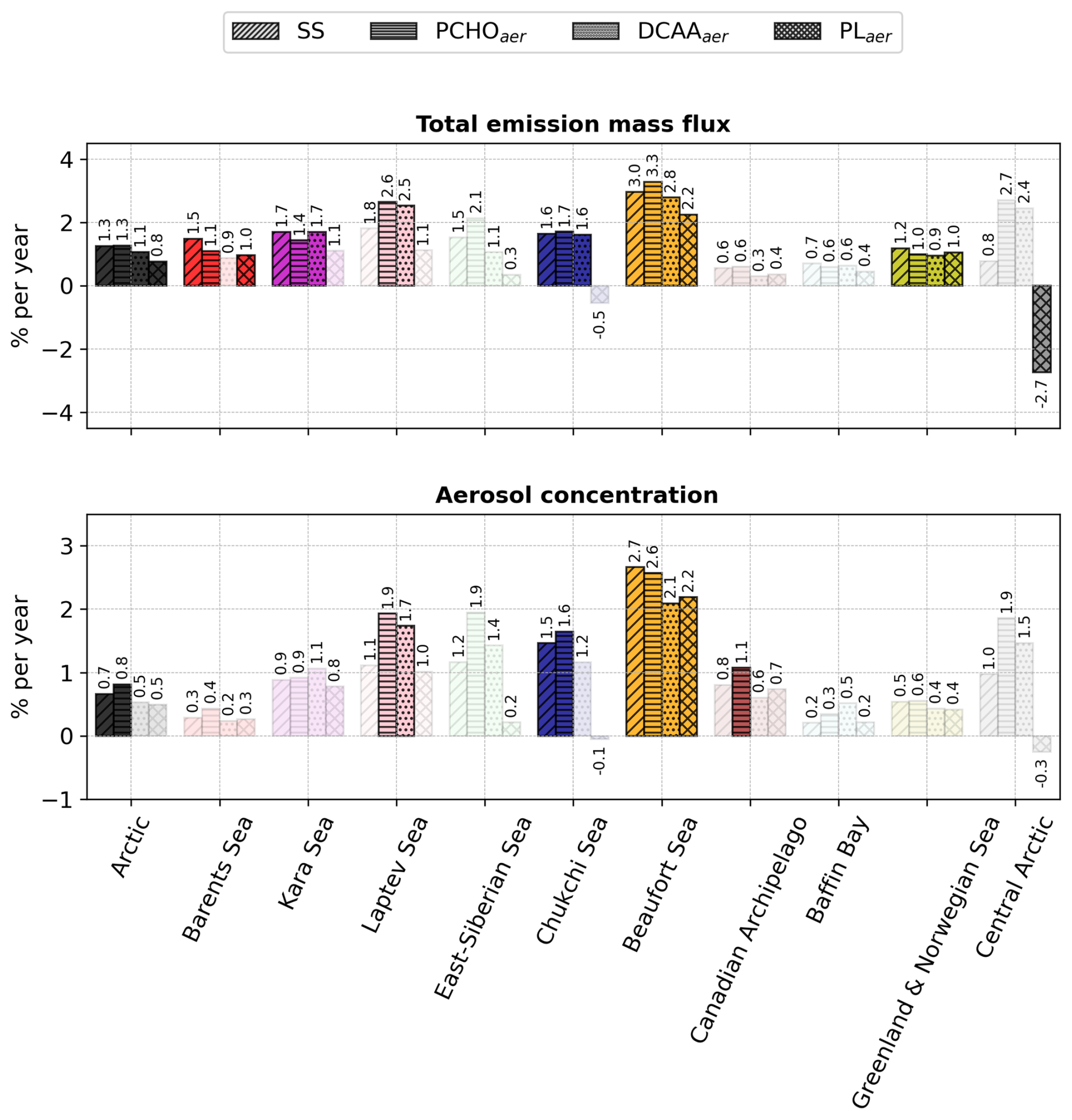
Figure 10 Bar plot of the percentage of change per year of total emission flux and near-surface mean aerosol concentration of marine species for the Arctic and the subregions defined in Fig. 1 for July–August–September of the period 1990–2019. Values were calculated by normalising the slope of the trend analysis by the 30 year average value for every subregion. The values atop the bars are the corresponding percentage per year. The shaded bars represent the cases with no significant trend (Mann–Kendall test, p-value > 0.05).

To analyse the relative changes per year of each marine species over the 30 years across Arctic subregions, Fig. 10 shows the percentage of change per year of total emission flux and aerosol concentration. For the whole Arctic, SS emissions increased by 1.3 % yr⁻¹, which represents 6.8 × 10⁻³ $\mathrm{Tg}{\mathrm{season}}^{-\mathrm{1}}{\mathrm{yr}}^{-\mathrm{1}}$ (see also Fig. I1a). Among PMOA aerosols, PCHO_aer present the strongest relative increase compared to DCAA_aer and PL_aer. For the Arctic subregions, despite the absolute values being the highest for the Barents, Greenland, and Norwegian waters (Fig. 9b–e), the relative increase is stronger for the inner Arctic seas. The Beaufort and Laptev seas have strong positive values, ranging between 2.2 and 3.3 % yr⁻¹. Aerosol concentration trends, on the other hand, are only statistically significant for all species in the Beaufort Sea. Besides this region, SS is only relevant for the whole Arctic and Chukchi Sea, while PCHO_aer trends are also significant in the Canadian Archipelago and Laptev Sea. Note that, given the complex transport and deposition processes that aerosols undergo once emitted, the trends of aerosol concentration do not necessarily reflect those of the emission fluxes. They are smaller in magnitude, spanning from 1.1 to up to 2.7 % yr⁻¹ for the Arctic subregions. For the Arctic, quantities are slightly weaker than for the emissions and only an increase of 0.6 and 0.7 % yr⁻¹ occurs for SS and PCHO_aer, respectively. Note that PCHO_aer is generally the organic group with the most prominent augment across Arctic subregions. Conversely, during the early melting season (April–June), while statistically significant trends were barely apparent in aerosol concentrations, upward emission trends for some species are observed in the Barents, Norwegian, Kara, Laptev, and Chukchi seas. Values tend to decrease for the Canadian Archipelago and Baffin Bay (Fig. H4). Among all biomolecules, PCHO_aer is the only group with a trend for the whole Arctic, with a relative change exceeding that calculated in the summer.

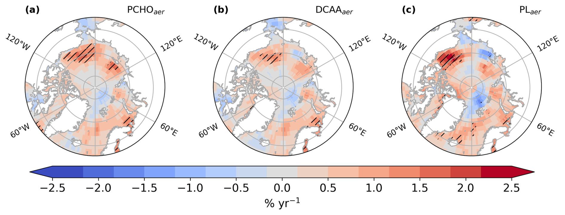
Figure 11 Maps of annual percentage variation in atmospheric burden for (a) PCHO_aer, (b) DCAA_aer and (c) PL_aer during July–August–September, derived from ECHAM6.3–HAM2.3 simulations covering 1990–2019. Hatched regions denote statistically significant trends (Mann–Kendall test, p-value < 0.05).

Finally, we describe the trends in marine organic aerosol burden and compare the relative increases among different species (Fig. 11). Their spatial distribution resembles the emission and aerosol concentration patterns (see Fig. 8d and e). For PCHO_aer, the burden's relative rise reached 1.8 % yr⁻¹ in the Chukchi Sea. In addition to this subregion, statistically significant trends are observed in the Beaufort Sea, parts of the Laptev Sea, and the Southern Barents Sea. Conversely, DCAA_aer shows fewer areas with significant trends, with its maximum increase also in the Chukchi Sea (1.5 % yr⁻¹). PL_aer exhibited stronger fluctuations, reaching up to 2.4 % yr⁻¹ in the Beaufort Sea, and also displayed significant patterns in parts of the Greenland Sea. Unlike other aerosol variables (Fig.10), regional average burdens did not show significant trends. Still, Fig. 11 verifies the presence of positive trends in marine aerosol burdens in regions with critical ice loss (Fig. 8).

5 Challenges of modelling PMOA

Observational records are too brief and geographically scarce to establish robust trends. The limited availability of marine organic seawater samples from Arctic field campaigns and the lack of aerosol-species resolved observations constrain further improvement of methods for computing ocean biomolecules and marine aerosol emissions in the polar region. This data scarcity is particularly evident in the species-resolved model outputs of the present study. What is presented here is therefore the best possible estimate of pan-Arctic and subregional conditions, given current data. Nevertheless, inherent uncertainties must be taken into account when evaluating the results.

The climate-driven sea ice reduction, with the subsequent appearance of wider open ocean areas, contributes to an increase in marine emissions. Aerosol–climate model studies agree on a further increase in the SS aerosol budget in the coming decades, with a relevant impact on cloud formation and cloud-radiative effects in the Arctic (Struthers et al., 2011; Gilgen et al., 2018; Lapere et al., 2023). Yet, large model uncertainties remain in the representation of marine organic aerosol sources and sea salt emission (Lapere et al., 2023). Accounting for all relevant aerosol-related processes represents a major challenge for models in the Arctic (Schmale et al., 2021; Whaley et al., 2022), especially for large-scale models (Ma et al., 2014). Moreover, aerosol source apportion, mixing, and removal mechanisms should be improved in models as they are the origin of significant uncertainties (Wang et al., 2013; Schmale et al., 2021; Whaley et al., 2022). Aerosol–cloud interaction and its impact on Arctic mixed-phase clouds remain highly uncertain, and considering them in models is difficult (Morrison et al., 2012). Furthermore, the representation of other important marine aerosol sources besides the open ocean could represent a limitation in most aerosol models. Recent findings by Lapere et al. (2024) highlight the need for further research on the SS emission from leads, as their contribution could be comparable to the averaged open-ocean SS fluxes. As observations have linked organic aerosols and biological components in seawater samples from leads (May et al., 2016; Kirpes et al., 2019), neglecting this marine source in models could potentially underpredict the actual PMOA concentration over the ice pack.

Importantly, the source functions to account for marine emission are parameterised in various ways, essentially following the correlation between the surface wind speed and the sea spray fluxes (Mårtensson et al., 2003; Gong, 2003). Nevertheless, the performance of SS emission schemes in models varies over a wide range (Neumann et al., 2016; Barthel et al., 2019; Lapere et al., 2023). These differences gain relevance in the PMOA fluxes estimation, since the SS scheme and model configuration determine the emission patterns and PMOA budget (Leon-Marcos et al., 2025).

In the representation of marine biogenic emissions, some challenges arise in terms of PMOA components. Firstly, DOC sources in seawater encompass many other generation mechanisms than phytoplankton carbon exudation alone (Carlson, 2002). Hence, ocean concentration of organic aerosol precursors could slightly diverge from our results, depending on the approach to modelling ocean organic groups (Burrows et al., 2014; Ogunro et al., 2015). Secondly, despite being integrated in the FESOM-REcoM model as a tracer, a parameterization to account for the aerosolisation of TEP or their enrichment in aerosols has not been developed and therefore, not considered here. To our knowledge, the implementation of marine gel-like particles has not been included in aerosol–climate models. Nevertheless, given the observational evidence of their contribution to marine Arctic aerosol and CCN (Leck et al., 2002; Leck and Bigg, 2005a; Orellana et al., 2011; Leck et al., 2013), this topic is worth exploring in future research. Lastly, other components that we neglect are marine microorganisms and bacterial cells, which could also be transferred to aerosols through bubble bursting (Bigg and Leck, 2001a; Fahlgren et al., 2015; Zinke et al., 2024), in addition to the potential atmospheric biochemical activities of these airborne microorganisms (Matulová et al., 2014; Ervens and Amato, 2020; Zeppenfeld et al., 2021, 2023). Despite these shortcomings, the current study's results reflect the major trends based on the current state of knowledge.

6 Summary and conclusions

As Arctic sea ice continues to melt, elucidating the response of marine organic aerosol emission is important, as they are a potentially important climate factor, particularly at high latitudes. In this study, we investigated the distribution patterns and seasonality of three main marine biomolecule groups in the Arctic Ocean: dissolved carboxylic acidic containing polysaccharides (PCHO), dissolved combined amino acids (DCAA), and polar lipids (PL). These components are included within the model ECHAM-HAM as aerosol tracers to account for the emission, transport, and interactions with clouds and radiation.

The geographical distribution of biomolecule groups depends on the production and loss mechanisms considered in their computation. The physicochemical characteristics of organics in seawater determine their transfer to aerosols. PL group is the most relevant to PMOA and the occurrence in seawater concentrates mostly in coastal regions with river mouths, which provide nutrients to the Arctic seas. Seasonal patterns of the marine biomolecules and organic mass fraction in nascent aerosols have a remarkable seasonality. Maximum modelled contributions of the three organic groups typically occur between May and July. The distributions of marine aerosols and their analogous in seawater strongly vary across Arctic subregions. The diversity is determined by riverine nutrient supply, sea ice conditions and ocean vertical mixing.

The PMOA emission fluxes were also analysed and tend to be stronger in the North Atlantic during winter (January–February–March), spreading towards the central Arctic as sea ice melts in summer. Total PMOA emission mass flux and atmospheric burden are 5.7 × 10⁻² Tg yr⁻¹ and 1.6 × 10⁻⁴ Tg, respectively. Overall, aerosol quantities have risen for 2005–2019 with respect to the preceding fifteen years. This increase across the Arctic varies by species group, influenced by regional dependencies, differences in bloom peak timings, and the efficiency of atmospheric aerosol wet removal.

As PMOA is emitted together with SS, its distribution generally matches that of SS fluxes. Nevertheless, the seasonality of Arctic subregions shows the critical influence of marine biological activity, resulting in a bimodal seasonal distribution, in contrast to the unimodal Arctic-average seasonal distribution of SS emissions. PMOA fluxes peak initially in May, driven by the contributions from the Greenland, Norwegian, and Barents Seas, and then decay towards June, reaching a minimum in SS fluxes. This is followed by a slightly higher maximum in September, concurring with the lowest SIC in the inner Arctic seas. The PMOA patterns are influenced by surface winds, open ocean fraction and biomolecule ocean concentrations, and to a lesser degree by SST variations. The relationship between emissions and their drivers displays a marked seasonal dependence, with the strongest associations occurring with surface winds in summer (July–September) and with OMF, used here as a proxy for marine biomolecule levels, in spring (April–June).

The 30 year historical Arctic trends demonstrate that the negative changes in sea ice concentration and changing primary production significantly impact phytoplankton exudation. While a rise in total marine biomolecule mass was detected in most Arctic inner seas, a decreasing or contrasting trend occurs in the outflow regions. In terms of aerosols, summer (July–August–September) emission flux anomalies exhibit large interannual variations, with a general tendency to increase with declining sea ice for the second half of the study period. As for the ocean, PMOA trends have noticeable differences among Arctic subregions, with predominantly positive changes. PMOA groups show a variable response. We found that the Arctic total emission fluxes of PL_aer, DCAA_aer and PCHO_aer have increased by 2.6 × 10⁻⁴, 6.8 × 10⁻⁶ and 1.7 × 10⁻⁶ $\mathrm{Tg}{\mathrm{season}}^{-\mathrm{1}}{\mathrm{yr}}^{-\mathrm{1}}$, respectively, since 2019. This represents a relative change of 0.8, 1.1 and 1.3 % yr⁻¹ for each group.

The results of this modelling study indicate that PMOA emissions are sensitive to the sea ice retreat and changes in marine primary productivity. The heterogeneous evolution of PMOA species from 1990–2019 suggests that the individual components of PMOA could have different influences on cloud and precipitation formation. Our work provides a model setup, which accounts for different marine organic aerosol groups, that will be extended to consider other marine sources and aerosol–cloud interaction processes in upcoming works. Considering the distinct properties of cloud condensation and ice nucleation could have varying impacts on cloud formation and associated climate effects. In this study, we found that PCHO followed by DCAA held the most prominent relative changes in aerosol quantities for the Arctic Circle and most subregions. Due to the enhanced ice-nucleating activity associated with these groups, we can speculate that their contribution to INP will also experience some increase, potentially leading to a positive cloud radiative effect.

Appendix A: List of abbreviations

Table A1 Index of abbreviations for the most significant aerosol and marine compounds studied here.

Appendix B: Phytoplankton and biomolecule carbon concentration

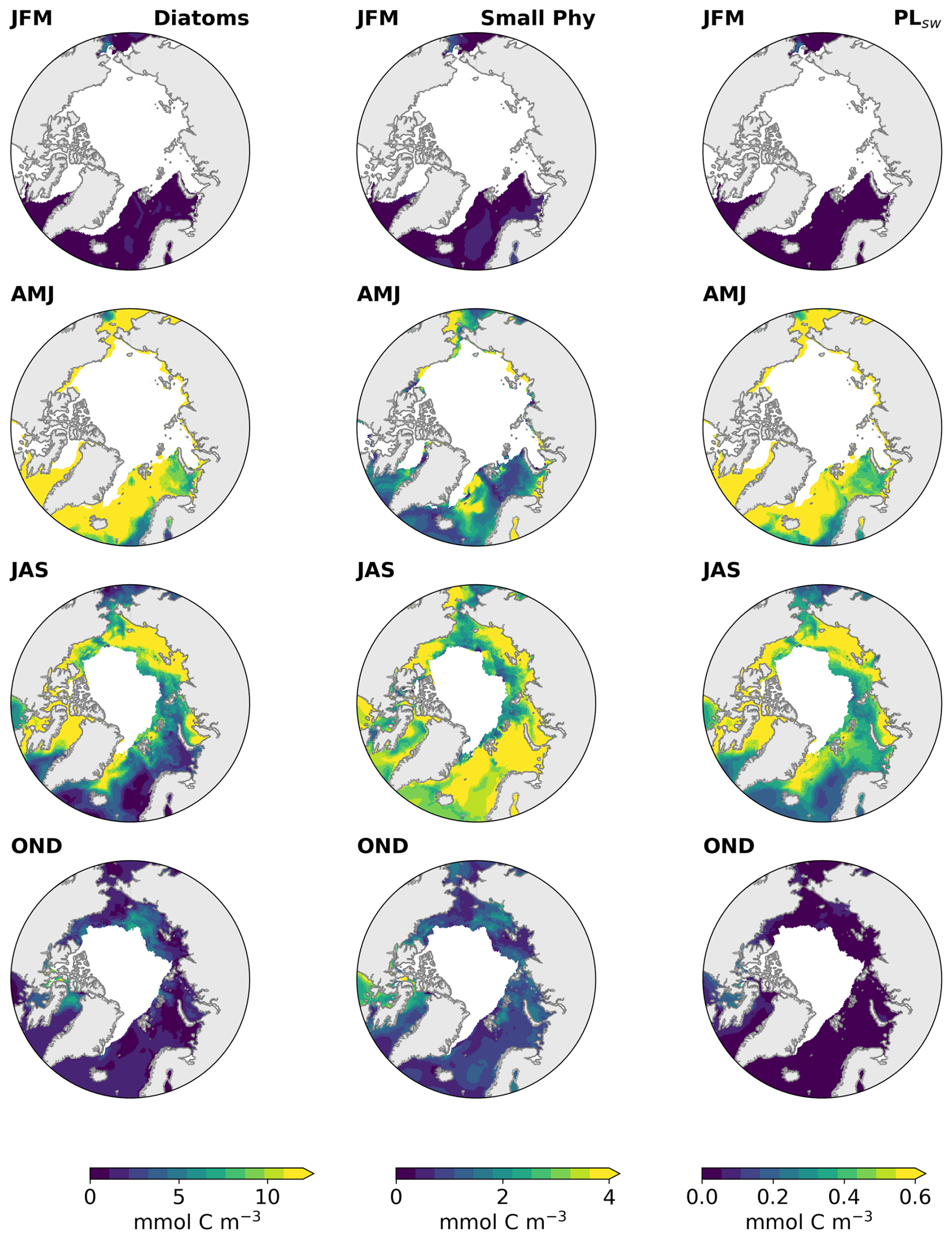
Figure B1 Maps of the carbon concentration of phytoplankton groups simulated by REcoM, Diatoms (left panel), small phytoplankton (middle panel) and PL_sw for January–February–March (JFM), April–May–June (AMJ), July–August–September (JAS) and October–November–December (OND) for the period 1990–2019 and sea ice free ocean conditions (SIC < 10 %).

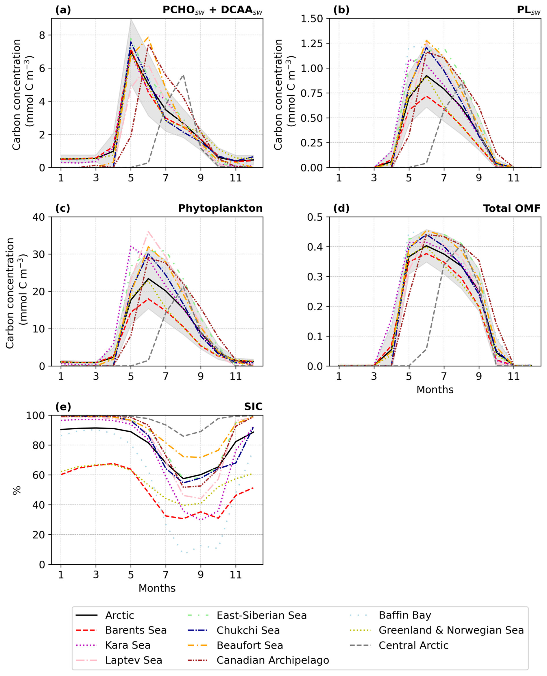
Figure B2 Seasonal climatology of (a) ocean carbon concentration of PCHO_sw + DCAA_sw, (b) PL_sw and (c) phytoplankton, (d) total OMF with sea ice free ocean conditions (SIC < 10 %) and (e) SIC modelled by FESOM for the period 1990–2019 averaged over the Arctic Ocean (66–90° N) and Arctic subregions in Fig.1.

Appendix C: Ocean biomolecule annual seasonality

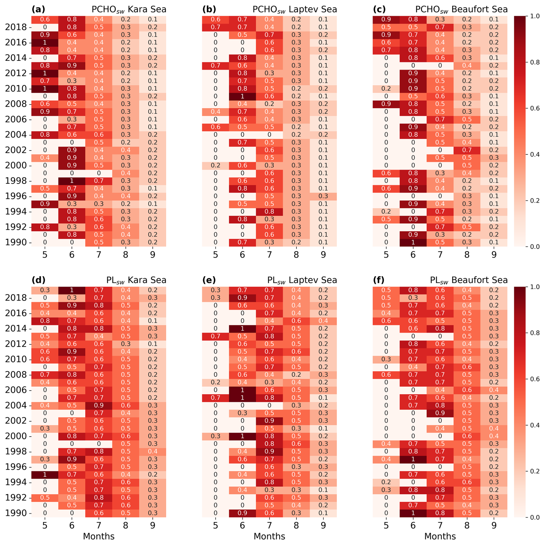
Figure C1 Annual seasonality of normalised averaged ocean biomolecule concentration for (a–c) PCHO_sw and (d–f) PL_sw for the (a, d) Kara, (b, e) Laptev and (c, f) Beaufort seas over the period 1990–2019 considering sea ice free ocean conditions (SIC < 10 %; Arrigo et al., 2008).

Appendix D: Arctic trends of DCAA

Figure D1 Arctic trends of DCAA_sw ocean concentration for April–May–June and July–August–September of the simulated period 1990–2019. The hatching indicates the areas over which trends are significant (Mann–Kendall test, p-value < 0.05). The green contour line depicts the average season 10 % sea ice concentration. The minimum seasonal SIC is also shown in shaded grey, occurring in June for April–May–June 2016 and in September 2012 for July–August–September.

Figure D2 Maps of DCAA_aer emission flux for April–May–June and July–August–September of the simulated period 1990–2019 by ECHAM-HAM model. The hatching indicates the areas over which trends are significant (Mann–Kendall test, p-value < 0.05).

Appendix E: Regional ocean biomolecule trends for July–August–September

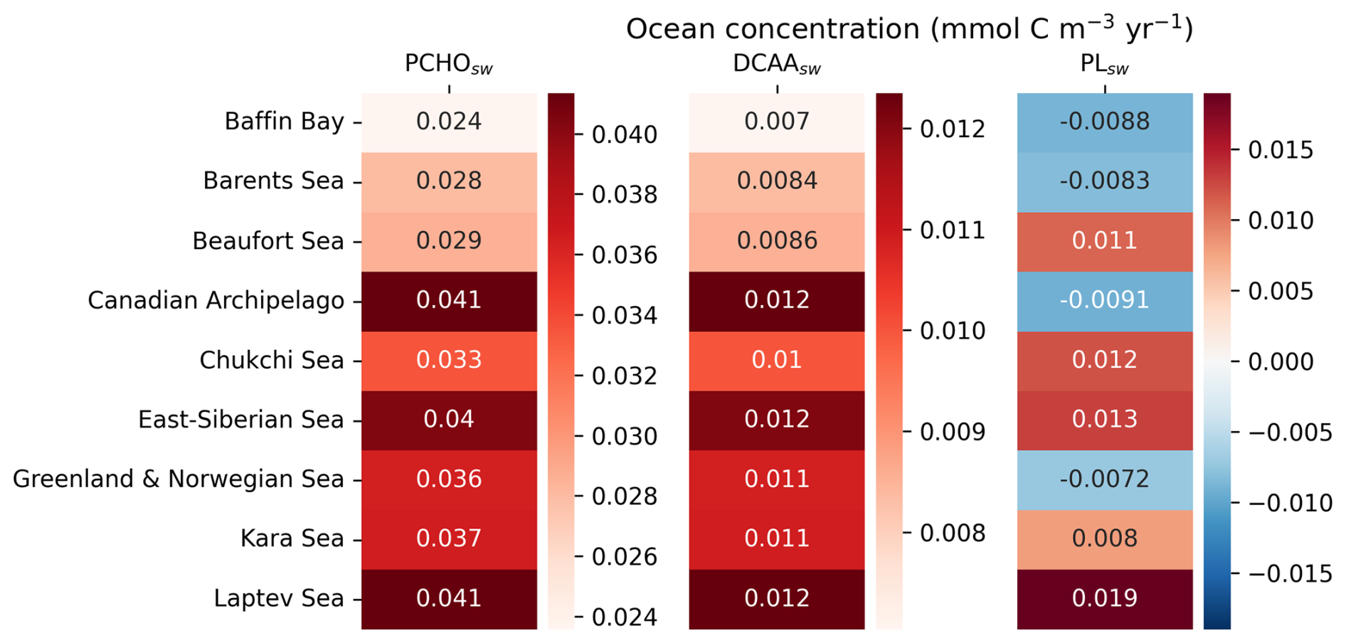
Figure E1 Absolute maximum trends for the Arctic subregions in Fig. 1 of biomolecule ocean concentration for July–August–September of the period 1990–2019. Only cases where the trends are significant (Mann–Kendall test, p-value < 0.05) are considered. Values were obtained after applying a mask with the minimum sea ice concentration shown in Fig. 6.

Appendix F: Differences between 1990–2004 and 2005–2019 for April–May–June

Table F1 Values of sea ice area, average PMOA concentration and total emission mass flux over the Arctic and Arctic subregions Beaufort Sea and Barents Sea analysed in Fig. 7 for 15 year periods, 1990–2004 (I) and 2005–2019 (II) for April–May–June. Seasonal emission totals are derived by adding daily values throughout the season across all grid cells in the region. The standard deviation of the multi-year average is shown in parentheses.

Appendix G: Arctic trends of surface winds and SST

Figure G1 Arctic trends of (a) surface wind speed sea and (b) sea surface temperature (SST) for July–August–September of the simulated period 1990–2019 from ECHAM-HAM model. Only grid cells where the trends are significant (Mann–Kendall test, p-value < 0.05) are considered.

Appendix H: Arctic trends for April–May–June

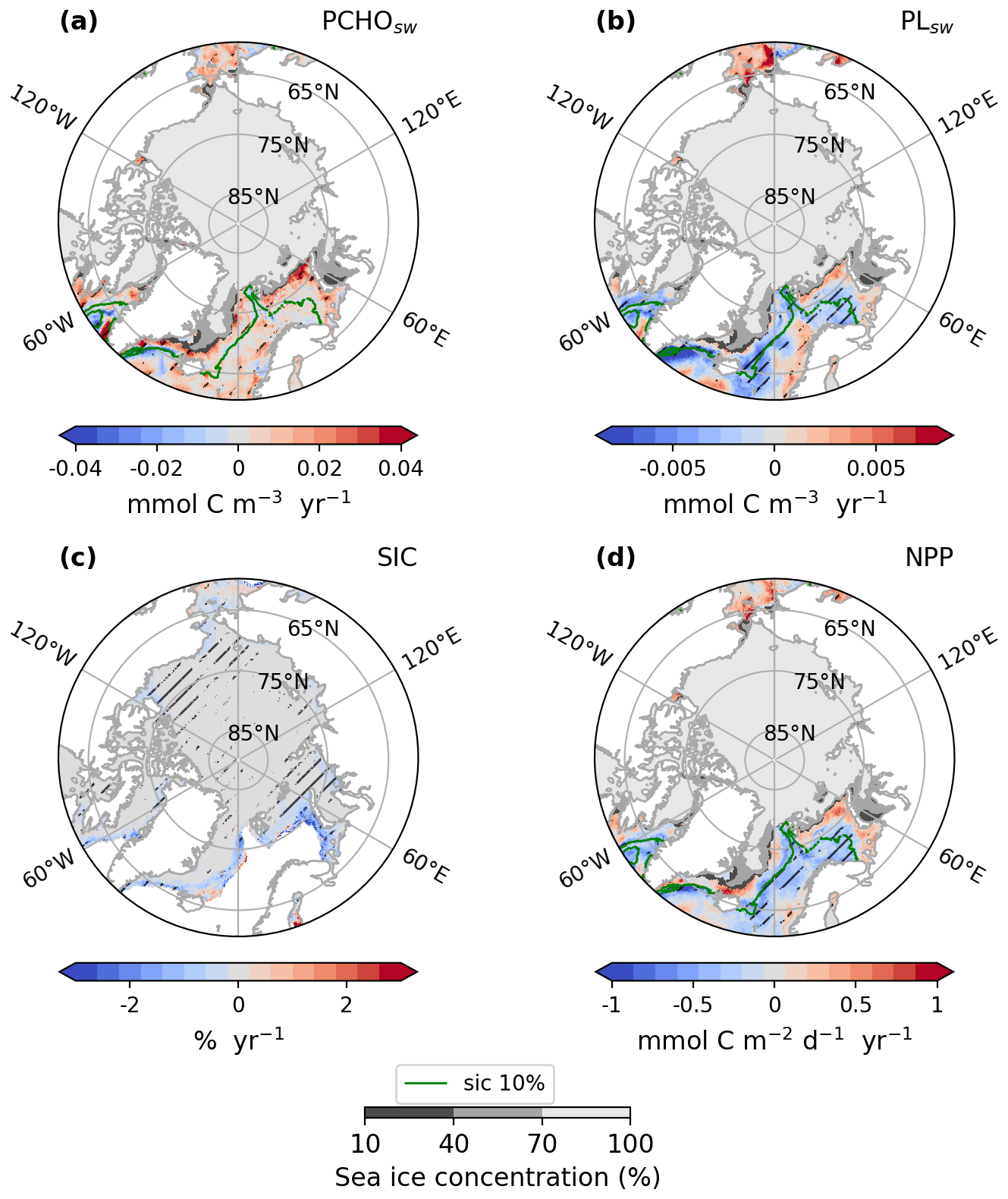
Figure H1 Arctic trends of (a) PCHO_sw and (b) PL_sw ocean concentration, (c) sea ice concentration and (d) net primary production from REcoM model for April–May–June of the simulated period 1990–2019. The hatching indicates the areas over which trends are significant (Mann–Kendall test, p-value < 0.05). The green contour line depicts the average season 10 % sea ice concentration. The minimum seasonal SIC for the period occurred in June 2016, and it is also represented in shaded grey.

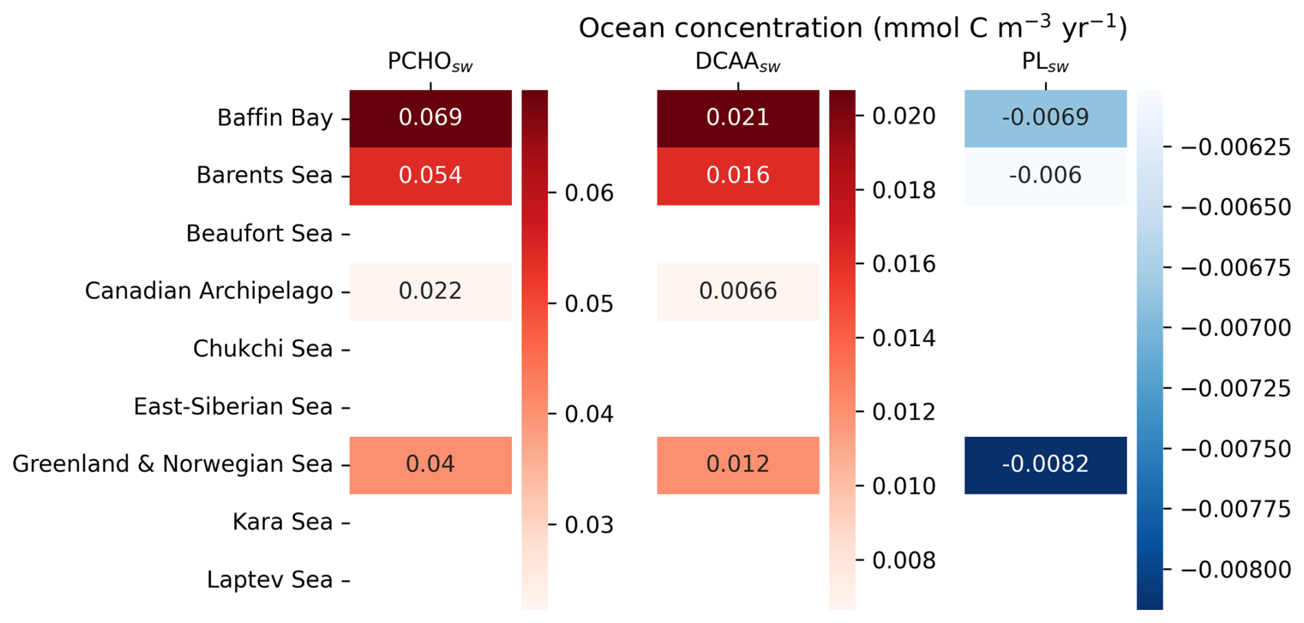
Figure H2 Absolute maximum trends for the Arctic subregions in Fig. 1 of biomolecule ocean concentration for April–May–June of the period 1990–2019. Only cases where the trends are significant (Mann–Kendall test, p-value < 0.05) are considered. Values were obtained after applying a mask with the minimum sea ice concentration shown in Fig. H1.

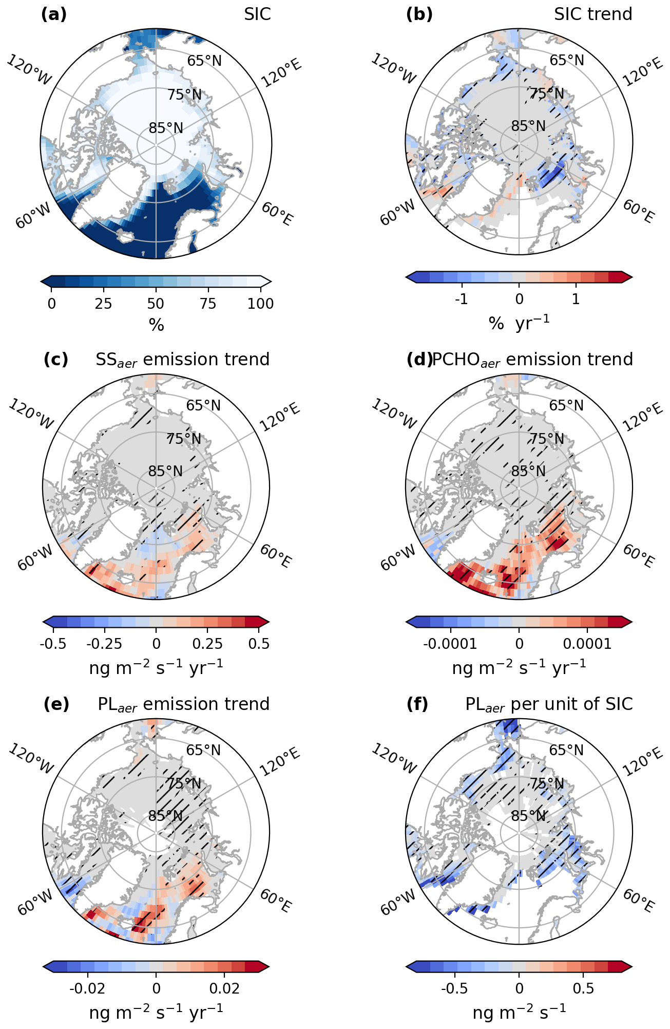
Figure H3 Maps of (a) average sea ice concentration (SIC), (b) trend of SIC, trends of emission fluxes of (c) SS, (d) PCHO_aer, (e) PL_aer and (f) changes of emission fluxes of PL_aer per unit of SIC for SIC > 20 %, for April–May–June of the simulated period 1990–2019 by ECHAM-HAM model. The trend of PL_aer per unit of sea ice was computed based on a linear regression model. The hatching indicates the areas over which trends are significant (Mann–Kendall test or t-test, p-value < 0.05).

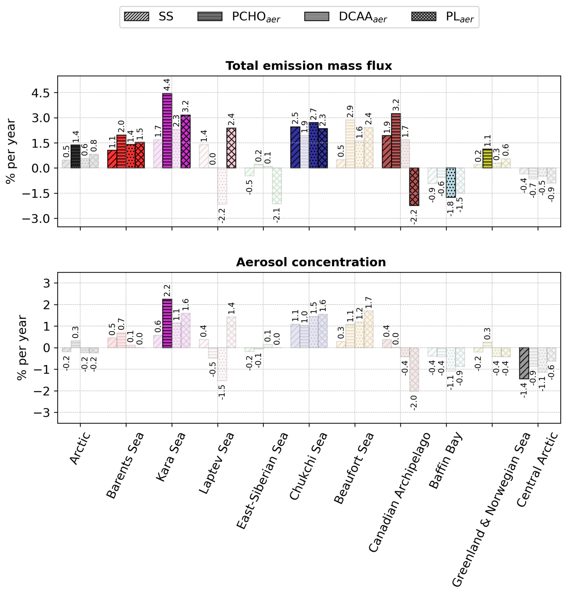
Figure H4 Bar plot of the per cent of change per year of total emission flux and near-surface mean aerosol concentration of marine species for the Arctic and subregions defined in Fig. 1 for April–May–June of the period 1990–2019. Values were calculated by normalising the slope of the trend analysis by the 30 year average value for every subregion. The values atop the bars are the corresponding percentage per year. The shaded bars represent the cases with no significant trend (Mann–Kendall test, p-value > 0.05).

Appendix I: Absolute total emission flux trend for July–August–September

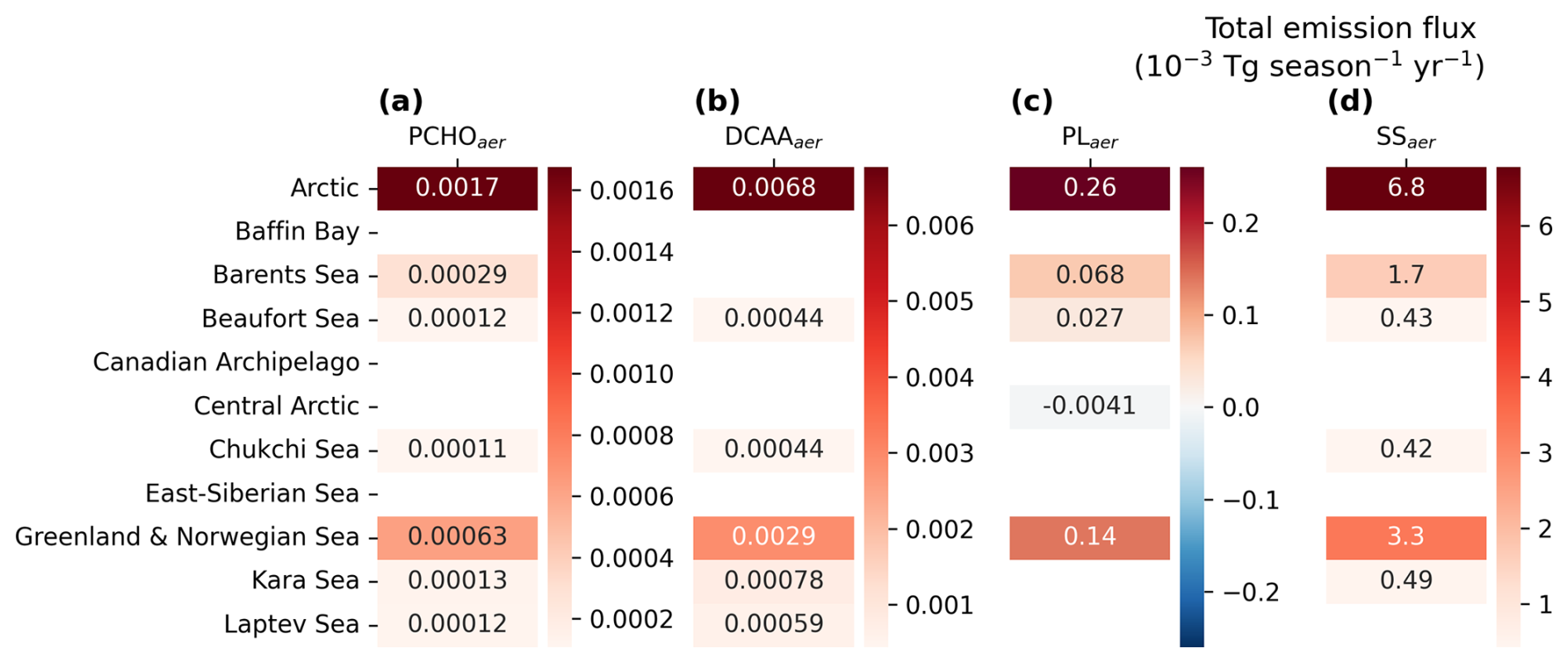
Figure I1 Heatmaps of trends over the Arctic and subregions defined in Fig. 1 for total emission mass flux of (a) PCHO_aer, (b) DCAA_aer, (c) PL_aer, and (d) SS simulated by ECHAM–HAM model for July–August–September of the period 1990–2019. Only regions where the trend was significant are included (Mann–Kendall test, p-value < 0.05).