
the Creative Commons Attribution 4.0 License.
the Creative Commons Attribution 4.0 License.
 | 06 Aug 2026
Assessing the stratospheric temperature response to volcanic sulfate injections by Mt. Pinatubo: insights from the Interactive Stratospheric Aerosol Model Intercomparison Project
Katharina Perny

Timofei Sukhodolov
Ales Kuchar
Pavle Arsenovic
Bernadette Rosati
Christoph Brühl
Sandip S. Dhomse
Andrin Jörimann
Anton Laakso
Graham Mann
Ulrike Niemeier
Giovanni Pitari
Ilaria Quaglia
Takashi Sekiya
Kengo Sudo
Claudia Timmreck
Simone Tilmes
Daniele Visioni
Harald E. Rieder
Some major volcanic eruptions, such as the one of Mt. Pinatubo in 1991, can inject large amounts of sulfur dioxide (SO2) into the stratosphere, leading to a volcanic aerosol cloud. This dense aerosol cloud induces a radiative heating of the stratosphere, causing ozone and water vapour changes, thereby altering middle atmospheric dynamics and chemistry. The scale of these impacts for varying injection amounts and heights on stratospheric temperature anomalies is still highly uncertain. Here we analyse specially designed chemistry-climate model experiments following the Historical Eruptions SO2 Emission Assessment Protocol (HErSEA) under the Interactive Stratospheric Aerosol Model Intercomparison Project (ISA-MIP). The results confirm our general understanding of the stratospheric aerosol forcing due to extra SO2 injection, while simultaneously highlighting structural differences between models. Overall, for the Pinatubo-like experiments the multi-model mean temperature anomalies agree well with meteorological reanalysis data sets, and we find that in most cases, differences between models are larger than differences for individual models across experiments with varying injection amounts and altitudes. Differences in transport, radiative transfer, and microphysics as well as the characterisation of aerosol size distributions, play a crucial role in the emergence of the spread in the modelled temperature response. Our results show further that the sensitivity of the stratospheric temperature response to model selection is also apparent in other MIPs. Hence, we argue for caution in attribution studies and the interpretation of stratospheric aerosol injection experiments relying on individual or few models.
- Article
(10622 KB) - Full-text XML
- BibTeX
- EndNote


Large volcanic eruptions can affect Earth's radiation budget and climate through injection of sulfur dioxide (SO2) and other gases into the stratosphere. Today, it is widely understood that the injected SO2 is converted to sulfate (SO4) aerosol within a few days to weeks, depending on the background chemical conditions, thereby thickening the stratospheric aerosol layer. This enhancement of the stratospheric aerosol layer scatters incoming shortwave (SW) radiation, absorbs solar near-infrared (near-IR) and terrestrial longwave (LW) radiation, and affects the chemical composition of the stratosphere (Robock, 2000). Due to the reduced insolation, Earth's surface is cooled, while the stratosphere is warmed through enhanced absorption by the aerosol particles formed (McCormick et al., 1995; Stenchikov et al., 1998; Lacis et al., 1992). These changes in atmospheric composition and thermal structure can have direct and indirect effects on stratospheric circulation, dynamics, and chemistry (Toohey et al., 2014; Diallo et al., 2017; Barnes et al., 2016; Zanchettin et al., 2022; Driscoll et al., 2012).
In the light of the well-documented cooling following volcanic sulfate emissions, stratospheric aerosol injection (SAI) has been discussed among a group of climate intervention strategies that might help limit global warming (Crutzen, 2006). In recent years substantial efforts have been directed to explore the feasibility of such intervention utilizing experiments with chemistry-climate models (CCMs) and Earth System Models (ESMs) (e.g., Tilmes et al., 2022; Richter et al., 2017) and analysing potential impacts on atmospheric dynamics (Aquila et al., 2014; Wunderlin et al., 2024), the environment and climate (Huynh and McNeill, 2024; Haywood et al., 2025). Although there are important differences between volcanic emissions and continuous SAI (Robock et al., 2013; Laakso et al., 2022), large volcanic eruptions remain the main natural analogue to evaluate how state-of-the-art aerosol microphysical models simulate SAI.
One of the last major volcanic eruptions that significantly affected global climate was the eruption of Mt. Pinatubo, a tropical volcano in the Philippines (15° N, 120° E), on 15 June 1991 (Robock, 2000). It was well observed by satellites (e.g., Long and Stowe, 1994; McCormick, 1987; Randel et al., 1995), airborne (e.g., McCormick et al., 1995; Pueschel et al., 1994; Borrmann et al., 1995; Deshler et al., 2003) and ground-based measurements (e.g., Nagai et al., 2010; Dutton and Christy, 1992; Antuña et al., 2002; Good and Pyle, 2004). The eruption injected SO2, water vapour and ash into the stratosphere. There are, however, substantial uncertainties associated with injection magnitudes and height (see detailed discussion in Quaglia et al., 2023). The global mean surface cooling following the Mt. Pinatubo eruption was estimated as up to −0.5 K, and a duration of the negative temperature anomaly of 18–36 months (e.g McCormick et al., 1995; Parker et al., 1996). Some uncertainties are, however, associated with these estimates, e.g. a recent study reports a weaker cooling of −0.2 K and also a shorter duration (Boretti, 2024). In contrast to surface cooling, pronounced stratospheric warming has been reported in the literature, with reanalyses (e.g., Fujiwara et al., 2015) and observations (e.g., Randel et al., 2016; Robock, 2000) showing the largest warming signals of up to 2–3 K over a year in the tropical lower stratosphere.
Recent research (DallaSanta et al., 2019) has shown that the warming of the tropical stratosphere following a tropical (Pinatubo-like) volcanic eruption leads to a strengthening of the polar vortices and a poleward shift of the jet in both hemispheres during winter. In addition, it was shown that precipitation is indirectly altered, namely through effects of stratospheric warming on atmospheric circulation (McGraw and Polvani, 2024; Simpson et al., 2019). In terms of chemistry in the middle atmosphere, ozone concentrations have been shown to be affected both by heterogeneous chemistry on the sulfate aerosol surfaces and by dynamical effects resulting from additional heating of the stratosphere (Aquila et al., 2013; Muthers et al., 2015; Dhomse et al., 2015). Ozone concentrations can increase or decrease depending on altitude and thermal environment as SO4 load effects heterogeneous reactions involving NOx, HOx, BrOx and ClOx and thereby alter atmospheric SW heating rates (Richter et al., 2017). Furthermore, increases in the stratospheric water vapour mixing ratio can be found due to the heating by volcanic aerosols leading to cold-point tropopause warming (Keeble et al., 2021; Kroll et al., 2021).
Over the last few decades, multi-model intercomparison projects (MIPs) have emerged as a widely used tool within the climate research community. These MIPs usually serve two purposes: (i) to provide outputs for process or trend studies under standardized protocols specifying boundary conditions and forcings, and (ii) to identify and explore biases between models and observations and inter-model differences. The Coupled Model Intercomparison Project (CMIP) supporting the Assessment Report Cycles of the Intergovernmental Panel on Climate Change (IPCC) and the Chemistry-Climate Model Initiative (CCMI and preceding MIPs) supporting the WMO/UNEP Ozone Assessment Reports constitute two of the most prominent MIPs. As these MIPs have not been designed to explicitly study the atmospheric/climatic impacts of volcanic eruptions or SAI, other MIPs such as the Interactive Stratospheric Aerosol Model Intercomparison Project (ISA-MIP; Timmreck et al., 2018), the Model Intercomparison Project on the climatic response to Volcanic forcing (VolMIP; Zanchettin et al., 2016) or the Geoengineering Model Intercomparison Project (GeoMIP; Visioni et al., 2023) have been initiated to address these concerns.
Within the ISA-MIP activity for interactive stratospheric aerosol CCMs (Timmreck et al., 2018), an intercomparison of simulations of the Pinatubo aerosol cloud (Quaglia et al., 2023) was made, to identify any common model-observation biases. Consistent also with findings from the 2006 Assessment of Stratospheric Aerosol Properties (ASAP) report modelling chapter (SPARC, 2022) one common model bias sees models tending to over-predict the optical depth of the Pinatubo cloud, compared to the benchmark Global Space-based Stratospheric Aerosol Climatology (GloSSAC)/Stratospheric Aerosol and Gas Experiment II (SAGE-II) gap-filled dataset. Dhomse et al. (2020) suggest the discrepancy may be due to the models not including volcanic ash, the effect shown to remove 43 % of emitted sulfur in the 2014 Kelud eruption (Zhu et al., 2020). Whilst there were substantial differences among model predictions, another persistent difference between the models and observations was that the simulations removed volcanic aerosol too quickly during the decay phase after peak optical depth. This result is in agreement with the VolMIP Tambora interactive stratospheric aerosol comparison (Marshall et al., 2018; Clyne et al., 2021), which found that key processes are missing in some models, leading to large inter-model spread in predictions. Zanchettin et al. (2022) investigated the surface temperature response in VolMIP and found good agreement among the models regarding the emergent surface cooling but differences in the radiative fluxes.
To date, however, no study has systematically addressed the stratospheric temperature response to volcanic aerosol in MIPs. Here we aim to close this gap by studying the stratospheric temperature response to volcanic aerosol forming after the Mt. Pinatubo eruption in the ISA-MIP models, and illustrating and explaining important model similarities and differences across models and between models and observations.
Our manuscript is structured as follows: The experimental design, information about the participating models in the relevant ISA-MIP experiments, data sources for the additional MIPs considered, as well as reanalyses and observational data sets are provided in Sect. 2. Section 3 shows model results of SO4 mass concentration and the stratospheric temperature response to different injection strategies, which are summarized and discussed in Sect. 4, which also presents ideas for directions of future community research.
In the subsequent subsections, we provide information on the experimental design of the ISA-MIP HErSEA experiments, building the foundation of this study, participating models, reanalysis products and observational data used to evaluate model outputs, data processing and data from further MIPs. For brevity we provide only information of direct relevance for the present study, for further details on the ISA-MIP HErSEA intercomparison we refer the interested reader to Timmreck et al. (2018) and Quaglia et al. (2023).
2.1 Model intercomparison project and experimental design
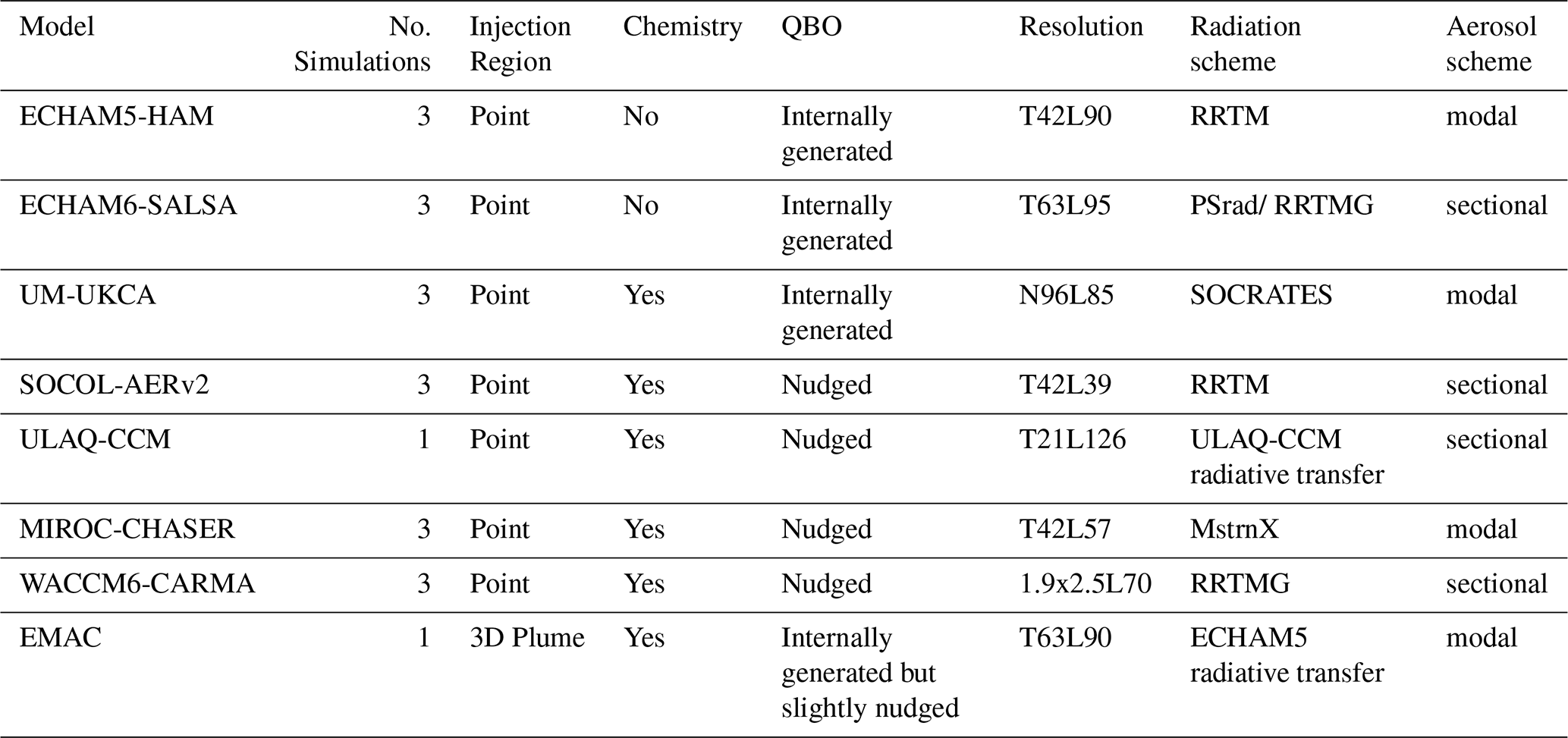
All models participating in the Interactive Stratospheric Aerosol Model Intercomparison Project (ISA-MIP) are using interactive aerosol microphysical modules and some also interactive chemistry (see Table 1). In the framework of the Historical Eruptions SO2 Emission Assessment (HErSEA) experiments, modelling groups performed transient Atmospheric Model Intercomparison Project (AMIP)-type runs of the Mt. Pinatubo eruption in which sea surface temperatures (SSTs) and sea ice extent are prescribed as monthly climatologies between 1991 and 1995 from the Met Office Hadley Center Observational data set (Rayner et al., 2003). Within HErSEA, five different emission scenarios were designed taking different amounts and altitudes of the volcanic SO2 injection into account. Three of these scenarios are described by injections at a medium altitude (between 21–23 km) but different amounts of SO2: low amount of 5 TgS (Low-22km), a medium 7 TgS (Med-22km) and high 10 TgS (High-22km). The medium-amount injection of 5 TgS has two additional scenarios with different injection altitudes: a shallow one at lower altitudes (18–20 km, Med-19km) and one over a deep altitude range (18–25 km, Med-18–25km). For brevity we refer to these experiments and the performing models hereinafter as ISA-MIP. We note in passing that EMAC model outputs are only presented in the analysis when discussing model similarities and differences in SO4 concentrations and transport, as EMAC did not fully adhere to the ISA-MIP experimental protocol (Quaglia et al., 2023).
The ISA-MIP simulation period spans from January 1991 to December 1995 (for UM-UKCA only until December 1993) and the eruption of Mt. Pinatubo is timed on 15 June 1991. SO2 injection is specified via a uniform vertical profile in a single grid cell at the respective altitudes close to the Mt. Pinatubo location (15° N, 120° E). The precision is defined by the specific vertical and horizontal model resolutions. The injection strategy differs only for EMAC (for which reason we flag it as EMAC* in the figures and tables), where volcanic SO2 is injected at a single point in time as 3D mixing ratio perturbations derived from satellite data using an inventory for the period 1990 to 2019 (https://doi.org/10.26050/WDCC/SSIRC_3, Brühl et al., 2021). The eruptions of Cerro Hudson (10 August 1991), Spurr (27 June 1992), and Lascar (18 April 1993) are included in EMAC and WACCM6-CARMA but they are not included in the remaining ISA-MIP simulations.
Following the experimental protocol, all models matched the observed post-Pinatubo QBO transition, either by nudging or from re-initialising from a prior control run. This ensures a consistent QBO state across different models, minimizing the effect of model-specific QBO dynamics on model spread on aerosols. Since the main focus of the HErSEA experiment was to improve our understanding of the long-term evolution of the Pinatubo volcanic cloud (Quaglia et al., 2023; Timmreck et al., 2018), the modelling teams agreed that radiative effects of ash, water vapour and SO2, as mainly relevant in the initial weeks post eruption (Stenchikov et al., 2021; Abdelkader et al., 2023), could be excluded. For completeness, it shall be noted that these effects can be important. For example, fine ash, due to the additional radiative heating below the sulfate cloud, can affect the initial transport direction of the aerosol cloud and inclusion of this feature can help represent modeled transport better (Niemeier et al., 2009, 2021).
For each different injection setting a three-member ensemble was submitted, except for ULAQ-CCM and EMAC, which submitted only one realization. In the respective model description sections the generation of the ensemble members is described. Unless otherwise specified, the ensemble mean of models is shown in the results.
2.2 Participating models
2.2.1 ECHAM5-HAM
MAECHAM5-HAM (further ECHAM5-HAM) is based on the ECHAM5 global climate model (GCM) (Giorgetta et al., 2006) and is used as a high-top model in the middle atmosphere (MA) version. It is also interactively coupled to the aerosol microphysical model HAM (Stier et al., 2005). Simulations were performed with a horizontal resolution of approximately 2.8° in longitude and latitude, a spectral truncation at wave number 42 (T42), and 90 vertical layers up to 0.01 hPa (approximately 80 km). This allows for an interactive QBO simulation. The mass conservation during advection is ensured by the scheme used in ECHAM5 for transport calculations, as outlined in the work by Lin and Rood (1996). Present-day conditions are prescribed with a land-sea mask, SST, and sea ice. These values are set to climatological averages from 1950 to 2000, as described in Hurrell et al. (2008).
The HAM aerosol microphysical model (Stier et al., 2005) calculates sulfur oxidation and sulfate aerosol formation, including nucleation, accumulation, condensation, and coagulation processes. The width of the HAM modes has been adapted to conditions with a high sulfur load after volcanic eruptions. The aerosols are prescribed in three modes, nucleation, Aitken, and accumulation, with a fixed width (Niemeier et al., 2009).
HAM was also adapted to stratospheric conditions by applying simple stratospheric sulfur chemistry above the tropopause (Timmreck, 2001; Hommel et al., 2011). HAM prescribes monthly oxidant fields of nitrogen oxides, hydroxyl radicals (OH), and ozone, as well as photolysis rates of OCS, H2SO4, SO2, SO3, and O3. Sulfate has been coupled with the radiation scheme of ECHAM for SW and LW radiation. Nucleation processes are simulated with a parametrisation after Vehkamäki et al. (2002), further adapted to high stratospheric sulfur loads by including collision processes.
Further details are described in Niemeier et al. (2021). We note, that the ensemble members were produced by increasing stratospheric horizontal diffusion by perturbing the respective parameter between 1.0, 1.0001, and 1.001 and setting it at the beginning of the simulation in January 1991.
2.2.2 ECHAM6-SALSA
The ECHAM6-SALSA refers to the aerosol–climate model ECHAM6.3-HAM2.3-MOZ1.0 (Kokkola et al., 2018) with the sectional aerosol module SALSA. The host component is the ECHAM6.3 general circulation model (Stevens et al., 2013), which is interactively coupled to the HAM aerosol module. A T63L95 resolution was used, corresponding to a horizontal grid of approximately 1.9° × 1.9°. The vertical atmosphere was divided into 95 layers, extending up to 80 km. This resolution enables the model to capture the QBO in the tropical stratosphere, which plays a key role in stratospheric aerosol transport (Laakso et al., 2022). Similarly to ECHAM5, ECHAM6 employs the flux-form semi-Lagrangian transport scheme of Lin and Rood (1996) to simulate tracer advection.
The HAM aerosol microphysical model simulates the emissions, removal processes, and radiative properties of the major aerosol species: sulfate, organic carbon, black carbon, sea salt, and mineral dust. It also includes gas- and liquid-phase sulfur chemistry. Concentrations of OH and ozone are prescribed from a monthly mean climatology. Anthropogenic aerosol emissions follow the Community Emission Data System (CEDS) for the CMIP6 emission inventory, while sea salt and dust emissions are calculated online.
In the ECHAM6-SALSA, aerosol microphysical processes – including nucleation, condensation, coagulation, and hydration are represented by the sectional aerosol model SALSA. Aerosols are resolved into 10 size bins, with the seven largest bins further separated into soluble and insoluble fractions. A comprehensive description of SALSA is provided in Kokkola et al. (2018).
Ensemble members were generated by introducing slight perturbations (0.0001 %) to one of the model tuning parameters, namely the snow formation rate by aggregation, applied only in January 1991 for each ensemble member.
2.2.3 MIROC-CHASER
The global chemistry–climate model MIROC–CHASER (Sudo et al., 2002; Watanabe et al., 2011) consists of the Model for Interdisciplinary Research on Climate (MIROC) version 4.0 and the atmospheric chemistry model CHASER (Sudo et al., 2002) and the Spectral Radiation–Transport Model for Aerosol Species (SPRINTARS) (Watanabe et al., 2011). For this study, the model is set up with a 2.8° × 2.8° horizontal resolution and 57 vertical levels up to 52 km. With this vertical resolution, QBO is not internally generated. The simulated tropical zonal winds in the stratosphere (15° N–15° S, above 90 hPa) were nudged to the observations compiled by Free University of Berlin (Naujokat, 1986) with a relaxation time of 20 d. Tracer advection was simulated using the piecewise parabolic method (Colella and Woodward, 1984) and a flux-form semi-Lagrangian scheme (Lin and Rood, 1996).
The aerosol module SPRINTARS tracks sulfate aerosol with three modes (nucleation, Aitken, and accumulation) and uses the bulk approach for black carbon and organic matter, dust, and sea salt (Sekiya et al., 2016). Nucleation is based on Vehkamäki et al. (2002). Condensation and evaporation processes are calculated with the equilibrium gaseous sulfuric acid as a function of temperature using a model referred from Kulmala and Laaksonen (1990), while the coagulation process follows the same scheme as ECHAM5–HAM (Stier et al., 2005) with van der Waals interaction as formulated by Alam (1987).
The chemical scheme in CHASER includes 93 species, as well as 263 reactions. Sulfur chemistry is included in the form of 12 reactions, as well as 4 of the main sulfur species (SO2, SO4, DMS, OCS) (Sekiya et al., 2016).
The initial conditions for the three ensemble members were taken from a 20 year timeslice simulation.
2.2.4 SOCOL-AERv2
Solar Climate Ozone Links version 3 with the interactively coupled aerosol model AER version 2 (SOCOL-AERv2) is an aerosol-chemistry-climate built with MA-ECHAM5 as the general circulation model. It is run in T42 configuration with a horizontal resolution of roughly 2.8°, 39 height levels going up to ∼ 80 km and a time step of 15 min. With this vertical resolution, the QBO is not internally generated, but nudged instead. The transport scheme, described in detail by Lin and Rood (1996), conserves the mass and preserves the shape of water vapour and chemical species during advection. A comprehensive model description is given in Stenke et al. (2013) and Feinberg et al. (2019). For radiative transfer calculations SOCOL-AERv2 employs the SW parameterization of Fouquart and Bonnel (1980) on 6 wavelength bands and the Rapid Radiative Transfer Model (RRTM) (Mlawer et al., 1997), which uses the correlated-k method, on 16 LW bands. Sulfate aerosol microphysics is treated by the sectional sub-model AER that calculates nucleation, coagulation, condensation, evaporation, and sedimentation of aerosol particles. It utilizes 40-size bins with radii from 0.39 nm to 3.2 µm (Sheng et al., 2015). Chemistry is represented in the module MEZON that calculates the interactions of 89 species (e.g. oxygen, hydrogen, nitrogen, …) using 234 reactions, including the detailed sulfur cycle (Brodowsky et al., 2024) and heterogeneous reactions on sulfuric, as well as polar stratospheric cloud (PSC) aerosol particles.
The time step for aerosol, chemical and radiative processes is 2 h, however, 20 sub-steps are calculated for aerosol microphysics, yielding an effective interval of 6 min. A three-member ensemble has been generated by modifying the carbon dioxide mixing ratio boundary condition by ±0.5 % for 1 month.
2.2.5 ULAQ-CCM
The ULAQ-CCM (University of L'Aquila Chemistry Climate Model) is a global-scale chemistry-climate coupled model with a horizontal lat × lon resolution of 5° × 6° (T21) and 126 log-pressure vertical levels (approximate pressure altitude increment of 568 m), from the surface to the mesosphere (0.04 hPa). The QBO is not internally resolved, but nudged to observed values (Morgenstern et al., 2017). A flux-form Eulerian explicit transport scheme is used in the model, with a minimum vertical and horizontal diffusivity to ensure numerical stability.
The chemistry module includes medium- and short-lived species grouped in families (Ox, NOy, NOx, CHOx, Cly, Bry, SOx) and the major component of stratospheric and tropospheric aerosols (sulfate, nitrate, organic and black carbon, soil dust, sea salt, polar stratospheric clouds). This module includes seven sulfur species (OCS, CS2, DMS, H2S, SO2, MSA, H2SO4), as well as the most important long-lived species relevant for stratospheric chemistry (N2O, CH4, CO, hydrocarbons, CFCs, HCFCs, HFCs, PFCs, halons).
The microphysical code for aerosol formation and growth includes a gas–particle conversion scheme, homogeneous and heterogeneous nucleation, coagulation, condensation, and evaporation (Pitari and Mancini, 2002; Pitari et al., 2016). It also includes heterogeneous chemical reactions on sulfuric acid aerosols and polar stratospheric cloud particles; both heterogeneous and homogeneous upper-tropospheric ice particle formation processes are also included (Visioni et al., 2018). The aerosol module calculates the aerosol extinction, asymmetry factor, and single-scattering albedo, given the calculated size distribution of the particles for different wavelengths, and they are passed daily to the radiative transfer module.
The ULAQ radiative transfer module, operating online in the chemistry-climate coupled model, is a two-stream delta-Eddington approximation model used for chemical species photolysis rate calculation in UV-visible wavelengths and for solar heating rates and radiative forcing in UV-VIS-NIR bands (Toon et al., 1989). In addition, a companion broadband, k-distribution LW radiative module is used to compute radiative transfer and heating rates in the planetary infrared spectrum (Pitari et al., 2015). Absorption/scattering optical depths take into account Rayleigh scattering, absorption from O3, O2, NO2, SO2, H2O, CO2 and scattering/absorption from aerosol particles. Aerosol optical properties derived from the ULAQ-CCM sectional aerosol module are passed daily to the radiative transfer module, with appropriate wavelength-dependent values of Q-ext, g, and single scattering albedo, given the calculated size distribution of the particles.
2.2.6 UM-UKCA
The UM-UKCA simulations are performed using Global Atmosphere 4.0 configuration (Walters et al., 2014) of the UK Met Office Unified Model (UM v8.4) general circulation model, including the UK Chemistry and Aerosol chemistry–aerosol sub-model (UKCA). The GA4 atmosphere model has a horizontal resolution of 1.875° × 1.25° and 85 vertical levels (N96L85) from the surface to 85 km, gravity wave drag parametrization tuned to generate a realistic QBO, generated internally within the simulations. The transport scheme within GA4 is the semi-implicit semi-Lagrangian atmospheric dynamics, used to solve the non-hydrostatic fully compressible deep-atmosphere equations of motion (see Davies et al., 2005). Note that this differs from the ENDGAME dynamics used in the GA7 atmosphere model (Walters et al., 2019), the configuration used for UKESM1.0 (e.g., Sellar et al., 2019, 2020).
The UM-UKCA configuration here is adapted slightly from the basic GA4 described in Walters et al. (2014), with radiative effects from the interactive GLOMAP aerosol microphysics scheme, the GA4 model still based from the mass-based HadGEM2-ES aerosol scheme (e.g., Collins et al., 2011). The stratospheric ozone layer is also radiatively active in the simulations, from the interactive “CheST scheme” (“Chemistry of the Stratosphere and Troposphere”, see Archibald et al., 2020). The configuration of the GLOMAP aerosol microphysics module includes the adaptations for stratospheric aerosol described in Dhomse et al. (2014), with additionally heterogeneous nucleation of sulfate aerosol from meteoric smoke particles, as described in Brooke et al. (2017), and used equivalently in the GA4 UM-UKCA simulations in Marshall et al. (2018, 2019) and Dhomse et al. (2020).
The boundary conditions for the transient GA4 UM-UKCA Pinatubo simulations is described in Dhomse et al. (2020), using Greenhouse gas (GHG) and ozone-depleting substance (ODS) concentrations from Ref-C1 scenario from CCMI-1 (Morgenstern et al., 2017). The simulations were in atmosphere-only mode, specifying time-varying SSTs and sea ice concentrations through the post-Pinatubo period from the AMIP simulations for CMIP6 (obtained from https://esgf-node.llnl.gov/projects/cmip6/, last access: 25 March 2021).
The initialisations for the three ensemble members were selected from 20-year time-slice simulations that gave a QBO transition through 1991, approximately matching that of the ERA-Interim reanalysis (Dee et al., 2011), see Appendix A of Dhomse et al. (2020).
2.2.7 WACCM6-CARMA
In this study, the Community Earth System Model version 2.2 (CESM2.2; Danabasoglu et al., 2020) is configured with the atmospheric component of the Whole Atmosphere Community Climate Model, incorporating Middle-Atmosphere chemistry (WACCM6-MA; Gettelman et al., 2019; Davis et al., 2023), at a horizontal resolution of 1.9° × 2.5°, using the finite volume dynamical core (Lin and Rood, 1997). WACCM6-MA the high-top configuration of CESM, featuring 70 vertical levels and extending up to approximately 150 km. The QBO is not internally generated, but the tropical zonal winds are nudged to idealized observations between 4 and 86 hPa and 10° S to 10° N (Matthes et al., 2010) following Davis et al. (2023). The MA model includes comprehensive chemistry for the stratosphere, mesosphere, and lower thermosphere, while employing a simplified chemical mechanism in the troposphere. The scheme includes 59 chemical species, 217 gas-phase reactions, and 17 heterogeneous reactions.
Aerosols in both the troposphere and stratosphere (including black carbon, primary organic matter, secondary organic aerosols, sea salt, dust, and sulfate) are simulated using the sectional microphysics scheme of the Community Aerosol and Radiation Model for Atmospheres (CARMA; Yu et al., 2015; Tilmes et al., 2023). In this configuration, CARMA includes two aerosol groups: one representing internally mixed particles and another representing pure sulfate particles. Each group is resolved into 20 size bins, ranging from 0.05 to 8.7 µm for the mixed group and from 0.3 nm to 1.3 µm for the pure sulfate group. The model accounts for binary homogeneous nucleation of sulfuric acid and water, applied exclusively to the pure sulfate group using the Zhao scheme (Zhao and Turco, 1995), as well as condensational growth and evaporation of sulfuric acid for both groups. Coagulation processes are included within each group and between groups. Both aerosol groups are also subject to dry deposition, calculated using the Zhang et al. (2001) parameterization, and gravitational settling, with settling velocities determined according to Seinfeld and Pandis (1998), and wet deposition (see Tilmes et al., 2023).
Aerosol optical properties are computed using a core-shell Mie scattering model, which captures the layered structure of internally mixed particles in the mixed aerosol group, following the method of Yu et al. (2015). In this setup, black carbon and dust serve as the core materials, while the shell is composed of water and water-soluble components such as organics, sea salt, and sulfate. For the pure sulfate group, the Mie calculations assume homogeneous particles with no core and use the sulfuric acid weight percentage to determine the refractive index.
The three ensemble members were initialized from a spin-up simulation, using different years (1979, 1980, and 1981) for the initialization of the start date in the year 1980.
2.2.8 EMAC
EMAC consists of the general circulation model ECHAM5 and the Modular Earth Submodel System MESSy V2.52 (Jöckel et al., 2010) including Atmospheric Chemistry. We use a setup in the spectral resolution T63 (1.9°) with 90 layers up to 1 Pa (80 km) where the meteorology of the troposphere up to 100 hPa is nudged to the reanalysis ERA-Interim (now ERA5). SSTs and sea ice cover (SIC) are prescribed by the reanalysis. The QBO is internally generated but slightly nudged to observations compiled by the Free University of Berlin (relaxation time 2 months, based on Giorgetta and Bengtsson (1999). Species are transported with the semi-Lagrangian advection scheme of ECHAM5 (Lin and Rood, 1996). EMAC uses the radiative transfer of ECHAM5 with corrections of Thomas (2008) with 4 solar and 16 terrestrial IR bands. EMAC contains comprehensive gas-phase and heterogeneous chemistry. The applied aerosol module GMXE (Pringle et al., 2010) accounts for seven modes using log-normal size distributions (nucleation, soluble and insoluble Aitken, accumulation, and coarse modes, adjusted for stratospheric applications (Schallock et al., 2023)). Optical properties for the types sulfate, dust, organic carbon, black carbon, sea salt, and aerosol water are calculated using Mie-theory-based lookup tables for each mode consistent with the simulated size distribution of each mode. The resulting total optical depths, single-scattering albedos, and asymmetry factors are used in radiative transfer calculations, which feed back to atmospheric dynamics (especially ascent and descent).
The results from EMAC were taken from an existing 30-year transient simulation for comparison with satellite observations (Schallock et al., 2023). The 3D plume for sulfur injection by Mt. Pinatubo was derived from several weeks of SAGE-II data, leading to a spread over a latitude and altitude belt (ca. 20°, 3 km).
Table 1Main characteristics of models participating in ISA-MIP.
2.3 Observational data and reanalysis
2.3.1 REMAP-GloSSAC-2023
To assess the model-predicted heating of the stratosphere, we first analyse how the models differ in terms of volcanic sulfate, compared to a best-estimate observational dataset (REMAP-GloSSAC-2023, https://doi.org/10.3929/ethz-b-000713396, Jörimann et al., 2025). This was derived from the observational composite GloSSAC version 2.22 (GloSSACv2.22; NASA/LARC/SD/ASDC, 2022), which provides aerosol extinction coefficients on up to four wavelength bands. From these data, a unimodal log-normal aerosol size distribution with three free parameters can be derived. This was done by iteratively checking the error between theoretical and measured extinction coefficients for the entire realistic parameter space and selecting the best-fitting parameters, following the Retrieval Method for Aerosol optical and physical Properties in the stratosphere (REMAPv1; Jörimann et al., 2025). Thus, we produced monthly stratospheric fields of H2SO4 number density. These fields contain useful values up to 80° latitudinally and up to 39.5 km; however, GloSSAC provides only a high-altitude climatology above 27 km, as opposed to transient data, mostly based on the well-established SAGE II and III data. Earlier versions of REMAP were also used to create stratospheric aerosol forcing data for both CMIP6 and CCMI-2022 (Sect. 2.4).
2.3.2 Reanalysis
For evaluating the temperature response in the model simulations we use data from three atmospheric reanalyses, including the European Centre for Medium-Range Weather Forecasts (ECMWF) Fifth Reanalysis of the Atmosphere (ERA5; Hersbach et al., 2020), the Modern-Era Retrospective Analysis for Research and Applications, version 2 (MERRA2; Gelaro et al., 2017), the Japanese Reanalysis for Three Quarters of a Century (JRA55; Kobayashi et al., 2015). We use zonal temperature data on pressure levels (Martineau et al., 2018) from the Atmospheric Processes And their Role in Climate (APARC) Reanalysis Intercomparison Project (A-RIP) (SPARC, 2022) in this study. We are using the common grid version of this dataset, for which all diagnostics were interpolated horizontally onto a regular 2.5° × 2.5° grid for a subset of pressure levels that are common among all included reanalyses (Martineau et al., 2018).
2.3.3 Anomaly calculation
For SO4 concentrations, absolute values can be used instead of anomalies, as the background values are very low. The temperature signal, however, is influenced by various factors, such as the QBO, seasonal fluctuations, as well as large-scale phenomena such as the El Niño–Southern Oscillation (ENSO). Therefore, anomalies are better suited to illustrate the temperature response to the Mt. Pinatubo eruption.
For reanalyses multiple linear regression (MLR) following the approach by Fujiwara et al. (2015) is used, including two QBO indices (30 and 50 hPa monthly mean zonal wind time series around the equator), the observed Niño 3.4 index lagged by 4 months for the ENSO variability, the solar 10.7 cm flux data for the solar variability and linear trend. The effect of MLR compared to anomalies with respect to the mean of the period 1980–2000 (21 years centred around the Mt. Pinatubo eruption) can be seen in Fig. A1. While the median of the individual reanalysis distributions remains unchanged, the spread decreases substantially due to the MLR.
For the models, anomalies are built using their respective Control simulations. Since the ocean is not run interactively and QBO is nudged or re-initialized at the time of the eruption, their effects should be at least partially accounted for. Models with available wind data (ULAQ-CCM, MIROC-CHASER and SOCOL-AERv2) were used to analyse the QBO contribution to the temperature anomaly signal. This was achieved by comparing the anomalies (experiment minus Control) without QBO treatment and with QBO regressed out (model_QBO in Fig. A2). We can see that the effect is much smaller compared to the results for reanalysis using the mean of the period 1980–2000 (see Fig. A1), and therefore we do not apply MLR prior to calculating the anomalies of the models hereinafter.
2.4 Further MIPs
As noted above, the REMAP method which we use to derive mass-related stratospheric aerosol properties from observations is a successor to the algorithms used in CMIP6 and CCMI-2022 forcing preparations. After retrieving stratospheric aerosol size distributions the preparation of the forcing data sets for these MIPs included calculating not only the physical aerosol properties (effective radius, number density, and surface area density) but also the optical properties: aerosol extinction coefficient, single-scattering albedo and asymmetry factor – tailored to each model's spectral resolution. For CMIP6 these data were created with a similar best-fit algorithm – using, however, an earlier version of GloSSAC (v1.1) and selecting three out of four SAGE II wavelength channels. The data set was therefore termed SAGE-3λ and is described in detail in the Supplement to Jörimann et al. (2025). The forcing for CCMI-2022 was then based on a further extended and updated version of GloSSAC (v2.0). A key difference in the REMAP code applied to the different products was a parameterization used for regions, where data was scarce.
2.4.1 CMIP6-AMIP
We use monthly temperature data of 20 Climate Model Intercomparison Project Phase 6 (CMIP6) models (Eyring et al., 2016) within the historical AMIP experiment as listed with respective ensemble sizes in Table A1. The AMIP simulations span the period 1979–2014 and use observed SSTs and SICs, as well as prescribe other external forcings including volcanic aerosols, solar variability, GHG concentrations, and anthropogenic aerosols.
2.4.2 CCMI-2022
We use monthly temperature data from the nine CCMs participating in the historical simulations (REF-D1) of the Chemistry Climate Model Initiative 2022 (CCMI-2022; Plummer et al., 2021), which are listed together with the ensemble size of each model in Table A1. Only ensemble members created through different realisations and not by perturbing initialization, physics or forcing data were selected. The REF-D1 historical hindcast simulations use forcings that follow the observed historical conditions closely and cover the period 1960–2018. The simulations have prescribed monthly mean SSTs and SIC from the HadISST data set (Rayner et al., 2003). Even though the QBO should be nudged in the CCMI-2022 ensemble, Benito-Barca et al. (2025) found that in some models QBO is not nudged but internally generated and thus, differences between observations and models can evolve from non-synchronized QBO phases. Stratospheric aerosol surface area density (SAD) is prescribed from the same REMAP methods used to relate the size distribution to the 3λ aerosol extinctions from the SAGE-II satellite measurements (see Revell et al., 2017; Jörimann et al., 2025).
Given that the experimental design is designed to mimic the eruption of Mt. Pinatubo we start with an analysis of the time evolution of temperature anomalies in the tropics (Sect. 3.1). Thereafter, we expand the analysis to the space-time propagation of the volcanic aerosol plume (Sect. 3.2), the associated temperature response across the middle atmosphere (Sect. 3.3), and discuss the model sensitivity to changes in SO4 concentrations (Sect. 3.4). We progress by contrasting our findings for ISA-MIP with those for other recent MIPs (Sect. 3.5) and conclude with Sect. 4.
3.1 Tropical temperature anomalies
We start by illustrating in Fig. 1a the time evolution of the mean temperature anomaly in the tropical lower stratosphere normalized to June 1991 for the five HErSEA-experiments from the ISA-MIP project along with the multi-reanalysis mean (comprising ERA5, MERRA2 and JRA55). The stratospheric heating due to volcanic aerosols, as widely discussed in the literature (e.g., Robock, 2000; Stenchikov et al., 1998; McCormick et al., 1995), can be clearly seen in the reanalysis mean. After a short ramp-up period the heating peaks in September 1991 and stays relatively constant at approximately 2 K until January 1993. Thereafter, the tropical heating signal quickly diminishes and vanishes during boreal summer (JJA) 1993.
While the overall evolution of the temperature anomaly identified in the reanalyses is broadly reproduced by the multi-model mean across all experiments, the timing and persistence of the temperature anomaly peak differ from the pattern observed. Among the individual models the temperature anomaly signal fades faster than observed (already between June and October 1992) in ECHAM6-SALSA, ULAQ-CCM and MIROC-CHASER in all experiments. Regarding the magnitude of the temperature anomaly, we find a good agreement between reanalysis and the multi-model mean for all the experiments except the High-22km. In this experiment, the injection of 10 Tg of sulfur in the form of SO2 results in an overestimation of the temperature signal in most of the models and thus in the multi-model mean. For the other experiments we find, despite good agreement between the reanalyses and the multi-model mean, large differences between individual models. The envelope in temperature anomalies ranges between ECHAM6-SALSA, which shows the smallest temperature anomaly and the least difference across experiments and SOCOL-AerV2, which shows the strongest temperature signal and pronounced sensitivity to different injection magnitudes and altitudes.
Given the similarities at the 50 hPa level in Low-22km, Med-22km, Med-19km and Med-18-25km we expand in Fig. 1b the analysis to the vertical temperature anomaly in the tropical region for the time period with the strongest signal across models, which corresponds also to the initial peak in the reanalysis mean (September to December 1991). During this period, the reanalysis shows a peak in temperature anomaly of around 2 K between 30 and 40 hPa. While the multi-model mean captures the altitude of the peak and overall vertical distribution of the temperature anomalies well in most experiments, the magnitude is overestimated in all but Low-22km. This overestimation in the multi-model mean is due to the majority of models showing larger anomalies than observed, with several models exceeding the 3σ confidence interval of the reanalysis. With regard to the altitude of the peak temperature anomaly, experiment Med-19km marks an exception. In this experiment the anomaly peaks already around 50 hPa which can be explained by the low injection height. In summary, Fig. 1 shows that the multi-model mean, for most experiments, agrees well with the reanalysis mean in both time evolution and vertical distribution. Additionally, we find that differences between the models are larger than differences of individual models across experiments.
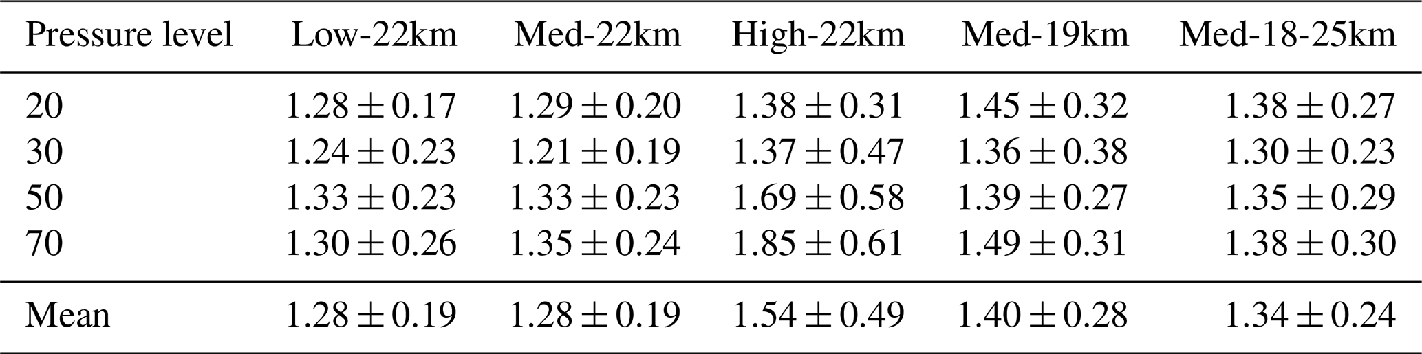
Therefore, to focus our study, we selected one of the five experiments as the core experiment for further analysis hereinafter, and retained the additional experiments for the discussion of important differences if they emerge. To select this experiment we used the Root Mean Square Error (RMSE) between the multi-model mean and reanalysis for the time evolution analysing the pressure levels with the strongest signal (see Table 2). As High-22km is overestimating the observed temperature response and the signal fades too fast in Med-18-25km, both experiments yield high RMSEs. While an overall best-agreeing experiment is not clearly emerging, the lowest mean RMSE is found for Low-22km and Med-22km. Given that Med-22km agrees better with reanalysis for most of the models than Low-22km (see Table A2), we selected Med-22km as our core experiment.
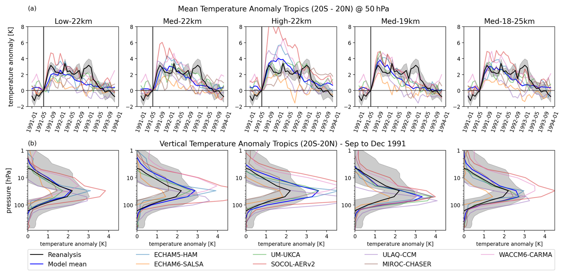
Figure 1Time evolution of the observed (multi-reanalysis mean) and model-derived tropical mean temperature anomaly normalized to June 1991 (a) and tropical vertical temperature anomaly for the period September to December 1991 (b). In all panels, the multi-model mean is provided as a blue bold line, and the grey shading indicates the ±3σ confidence bound for the reanalysis mean (black, bold).
Table 2RMSE for the time evolution of the observed (multi-reanalysis mean) and model-derived tropical mean temperature anomaly normalized to June 1991 for different pressure levels.
3.2 Space-time evolution of SO4 concentrations
Having set the scene by illustrating the large differences in temperature signal of the Mt. Pinatubo eruption across models, we turn to the model representations of the associated forcing. As discussed above, the stratospheric heating results mainly from the absorption of terrestrial LW and solar near-IR radiation. If the absorbing particle is much smaller than the wavelength, the absorption of terrestrial LW radiation and its stratospheric heating is proportional to the mass concentration of the sulfate aerosols (Van de Hulst, 1981; Murphy et al., 2021; Lacis, 2015). In the case of volcanic aerosols, the size distribution is comparable to near-IR wavelengths; thus, differences between modelled heating can originate from both mass concentration and size distribution and need to be considered in the subsequent analysis, even though the latter has less impact on the total absorption (Ramachandran et al., 2000; Stenchikov et al., 1998, 2021). If the aerosol radius is larger than ∼ 0.5 µm the absorption efficiency starts to increase strongly with increasing aerosol size (Laakso et al., 2022).
Quaglia et al. (2023) analysed the evolution of stratospheric aerosol optical depth, stratospheric sulfate burden, and aerosol properties (effective radius and SAD) in the ISA-MIP models. The main reason for disagreement among the models analysed in that study was differences in stratospheric transport. ECHAM6-SALSA, ECHAM5-HAM, and SOCOL-AERv2 showed too fast transport from the tropics to high northern latitudes, while for UM-UKCA, transport was confined to the NH. Transport in ULAQ-CCM was found to be too confined to the tropics, likely affected by a different vertical advection scheme in comparison to the other models based on the same dynamical core, ECHAM5 or ECHAM6. Additional factors influencing the tropical confinement were differences in vertical and horizontal resolutions and the definition of the tropical pipe. Overall, most of the models showed a preference for transport to the NH. Exceptions were EMAC, which has been nudged to reanalysis to represent observed tropospheric meteorological conditions, and UM-UKCA when emissions have been spread between 15° N and the Equator instead of point injection. These models showed a better agreement with observations regarding transport to the SH. For the other models, Quaglia et al. (2023) state as reasons for the lack of aerosol (transport) in the SH, the omission of (i) ash injection, which would be crucial in the early days/months to better reproduce the initial evolution of the aerosol cloud, as well as, (ii) aerosol emissions emerging from the Cerro Hudson eruption in August 1991 in the southern extratropics. Below we build on the findings of Quaglia et al. (2023) and extend their analysis with a focus on the time evolution and vertical propagation of SO4 concentrations and resulting temperature anomalies.
In Fig. 2 we show the time evolution of the zonal mean of SO4 concentrations exceeding 1 µg m−3 across the upper atmosphere. For this comparison, the REMAP-GloSSAC-2023 data serves as an observational reference. REMAP-GloSSAC-2023 shows increasing SO4 concentrations post-eruption in both hemispheres, which peak in the tropics until autumn 1991, and fade over the following year. In the models, zonal mean SO4 concentrations peak earlier (in late summer/early autumn 1991) than observed. Furthermore, the initial distribution differs widely among models. While for ECHAM5-HAM and ULAQ-CCM the SO4 concentrations are – similarly as for REMAP-GloSSAC-2023 – confined within a small and narrow fraction of the upper atmosphere, the SO4 plume in SOCOL-AERv2 and WACCM6-CARMA spreads across large parts of the lower and middle stratosphere. These initial differences across models can be attributed to the combined effect of SO2 conversion rates, transport and model vertical velocity (Niemeier et al., 2020). While some models (EMAC, ECHAM6-SALSA and SOCOL-AERv2) already start transporting SO4 through the shallow branch of the Brewer-Dobson Circulation (BDC) into higher latitudes shortly after the eruption, others, such as ECHAM5-HAM, ULAQ-CCM, and UM-UKCA, have SO4 more confined in the tropical pipe during the first months. By November 1991, all models show transport into higher latitudes; however, there are stark differences in transport pathways. Some models (e.g. EMAC, ECHAM6-SALSA, SOCOL-AERv2) show preferred transport through the shallow branch while others (e.g. UM-UKCA, WACCM6-CARMA, MIROC-CHASER) mainly transport through the deep branch until winter 1991/92. A special case is MIROC-CHASER for which SO4 concentrations are quickly transported into the northern subtropics (20–30° N) and then further towards the pole, with limited sedimentation and no apparent subtropical transport barrier.
Despite these model differences several similarities emerge. As discussed above, a preferred meridional transport to the NH can be identified in all models but EMAC, and UM-UKCA if emissions are spread between 15° N and the Equator (see Fig. A3), in agreement with Quaglia et al. (2023). For all ISA-MIP model realizations a net descent of SO4 concentrations begins in November 1991, likely reflecting the increased effective radius, and downward propagation of the SO4 plume emerges between late winter and early spring 1992. From May 1992 onward, the peak in SO4 concentration can be found over the northern polar region in all models, and only low SO4 values remain in the lower latitudes. While this is in broad agreement with REMAP-GloSSAC-2023 observational composite retrievals, the latter shows stronger transport to the southern hemisphere than the models. Despite the northern hemispheric transport preference of the models, both, low resolution models such as SOCOL-AERv2 and intermediate resolution models such as ECHAM6-SALSA and EMAC, perform well in comparison to REMAP-GloSSAC-2023 observations regarding the magnitude and transport patterns of SO4 concentrations. However, for ECHAM6-SALSA, the aerosol distribution between the hemispheres varies considerably across individual ensemble members, a feature highlighted in previous work (Quaglia et al., 2023; Laakso et al., 2016) pointing to strong sensitivities to the dynamic state at the injection grid point at the time of SO2 release.
Most importantly, Fig. 2 makes large differences in aerosol transport and concentrations across models apparent; thus, we investigate next how these relate to temperature signals and differences therein.
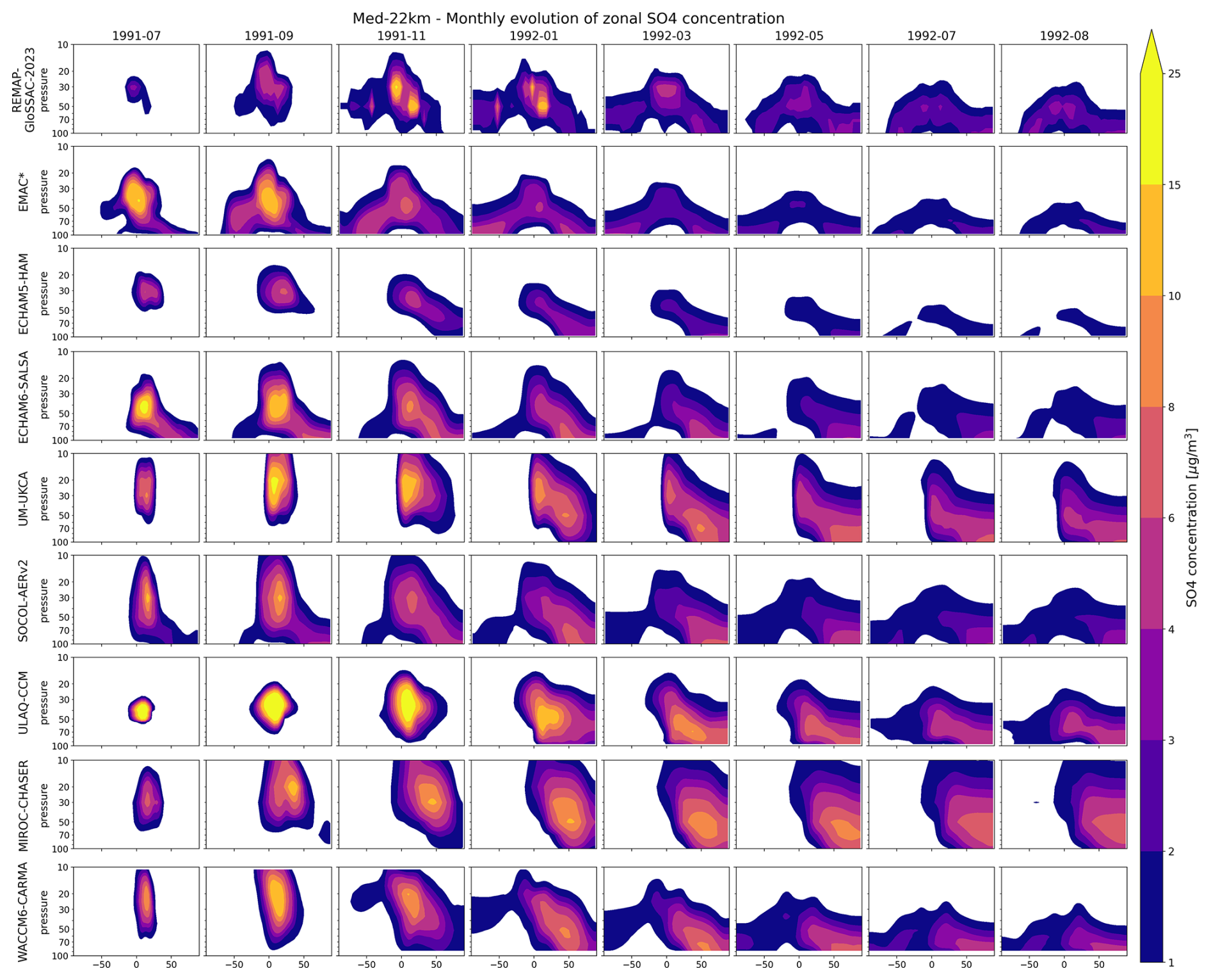
Figure 2Vertical evolution of zonal mean SO4 concentrations in experiment Med-22km for individual models, from July 1991 to August 1992 (bi-monthly; columns) in comparison with REMAP-GloSSAC-2023 observations (first row). Note, EMAC is flagged with * as it did not fully adhere to the ISA-MIP protocol, see Sect. 2.2.8.
3.3 Comparison of SO4 concentrations and temperature anomalies
The largest post-Pinatubo SO4 concentrations occurred in the tropics (e.g., McCormick and Veiga, 1992) and we first assess the progression of each model's volcanic sulfate in the 20° S–20° N region. To allow for a direct comparison of SO4 forcing and temperature anomaly we provide model-specific SO4 concentration contour lines in all panels of Fig. 3. First, we note that for both, the multi-reanalysis mean and REMAP-GloSSAC-2023 observations, a strong relationship between the progression of peak temperature anomaly and SO4 concentration appears in the spatial and temporal analysis. Second, in observations and in all models, the strongest temperature response occurs shortly after the eruption simultaneously with the highest concentrations in SO4. Third, the temperature signal decays over time as the SO4 plume propagates. Fourth, the strong correlation between temperature anomaly and SO4 concentration identified in observations is also present in all models; however, the magnitude, timing, temporal and vertical extent of the signal differ substantially between them.
For one thing, MIROC-CHASER and ECHAM6-SALSA stand apart from the other models and the observations: MIROC-CHASER as it does not show a descending temperature signal, and ECHAM6-SALSA as it does not show any significant temperature anomalies in Med-22km. The absence of a significant anomaly in ECHAM6-SALSA might be explained by a strongly varying aerosol distribution across the individual ensemble members (see discussion above). We note in passing that in experiments resulting in a stronger temperature signal, some significant anomalies emerge (see Fig. A4). Also, ULAQ-CCM differs markedly from the remaining models given the much faster descent and fade out of the temperature anomaly while its SO4 anomaly remains. From the remaining four models, the UM-UKCA ensemble mean appears to resemble the magnitude and pattern of temperature anomaly identified in the reanalysis. ECHAM5-HAM, SOCOL-AERv2 and WACCM6-CARMA agree with the observations regarding pronounced temperature anomalies but show in parts marked differences in magnitude, propagation and vertical extent. We attribute the deficiencies in reproducing observed patterns not solely to model issues in transport. This is exemplified as follows: while ECHAM6-SALSA and SOCOL-AERv2 agree well with reanalysis regarding the transport of the SO4 concentration plume (see Fig. 2), they over- (SOCOL-AERv2) or underestimate (ECHAM6-SALSA) the corresponding temperature anomalies.
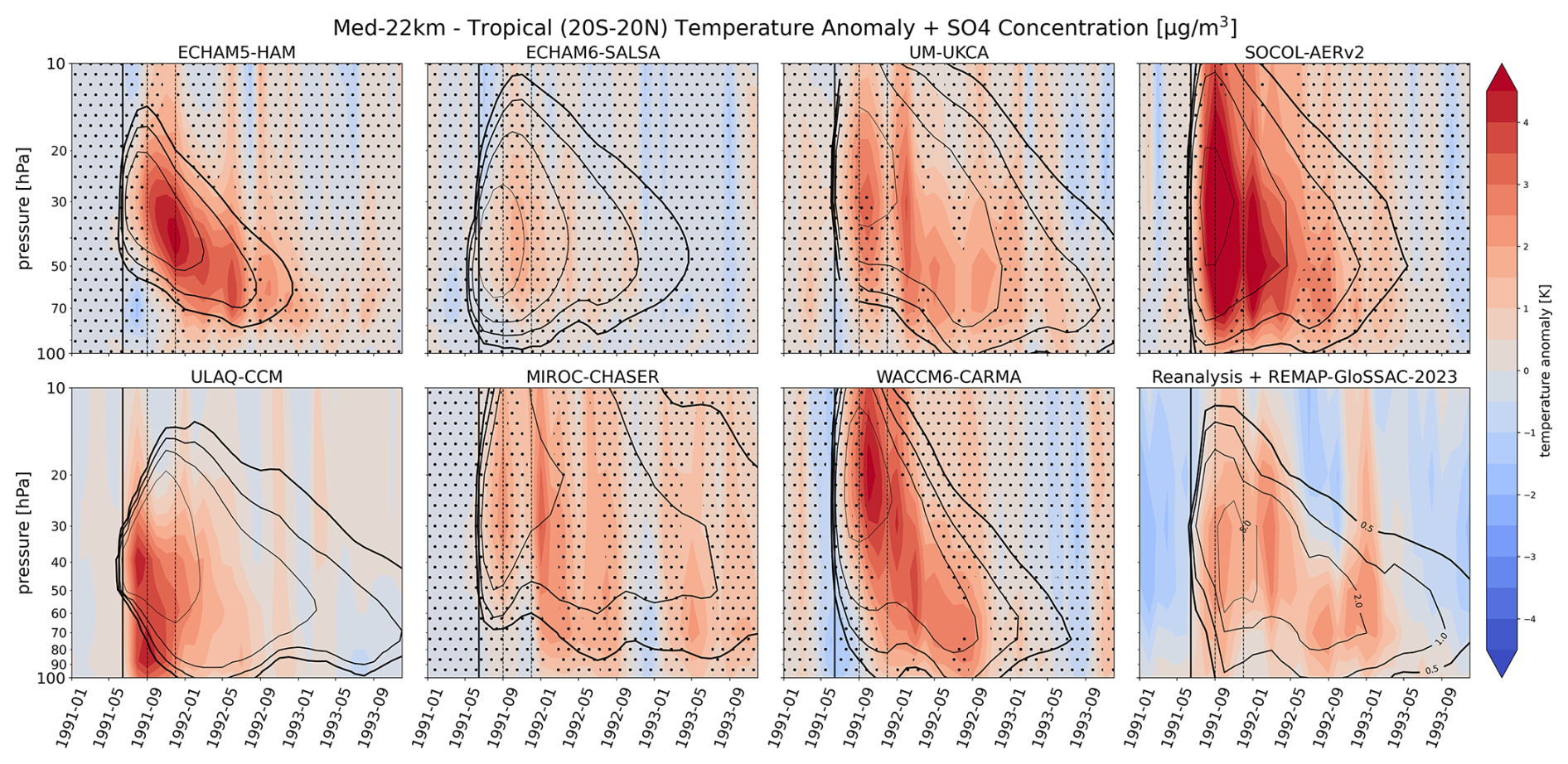
Figure 3Time evolution of the vertical temperature anomalies in the tropics (20° S–20° N) in experiment Med-22km for individual models. In all panels: SO4 concentrations are shown as contours (levels are 0.5, 1, 2, 5 µg m−3), dots indicate non-significant areas (p-value >0.05) for reanalysis and models with the exception of ULAQ-CCM where only one ensemble member is available, the thick black vertical line represents the Mt. Pinatubo eruption time while the thin vertical lines embed the time period September to December 1991. REMAP-GloSSAC-2023 SO4 concentrations are shown as contours in the reanalysis panel.
To investigate inter-model differences in the simulated Pinatubo aerosol vertical profile and associated temperature effects, we focus on the time period of the strongest temperature signal-to-noise ratio across models (September to December 1991) in Fig. 4. Starting with the observations, reanalyses highlight that the peak SO4 concentrations and temperature anomalies reside in the tropics (20° S–20° N) and across the lower and middle stratosphere (70–20 hPa). Further, the propagation of the volcanic signal over time can be clearly seen, i.e. hemispheric transport and descent (compare with Fig. 3).
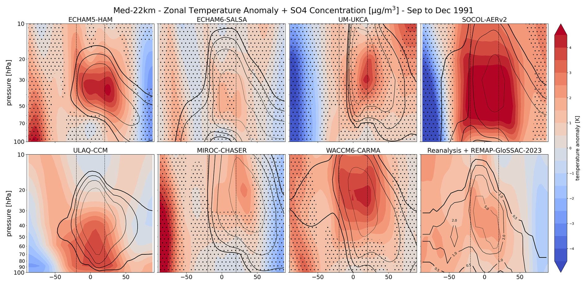
Figure 4Vertical zonal temperature anomaly in experiment Med-22km for the period September to December 1991 for individual models. In all panels: SO4 concentrations are shown as contours (levels are 0.5, 1, 2, 5 µg m−3), dots indicate non-significant areas (p-value >0.05), and the vertical lines show embed the tropical region (20° S–20° N). REMAP-GloSSAC-2023 SO4 concentrations are shown as contours in the reanalysis panel.
When probing the models, the observed relationship of the temperature anomalies and SO4 concentrations is present in all. Somewhat an exception is ULAQ-CCM, for which the location of the largest temperature anomalies can be found below the maximum of the SO4 concentrations. One may attribute this to a larger effective radius (exceeding 0.5 µm in radius in the tropics) in ULAQ-CCM compared to the other models in the lower stratosphere. However, given that WACCM6-CARMA also shows an tropical effective radius exceeding 0.5 µm while still smaller than ULAQ-CCM (see Fig. A6), such interpretation may not hold also pointing to limitations of effective radius in explaining the location of temperature anomalies. Also, MIROC-CHASER differs from the remaining models as its maximum SO4 concentrations and thus peak temperature anomalies emerge due to too strong transport (see Fig. 2) outside of the tropics. For the remaining models, the spatial structure of the SO4 concentrations agrees quite well with the reanalysis data. However, temperature responses across these models are very different in magnitude. Given the similarities in the SO4 concentrations, we do not attribute these differences to transport but rather to model specifics in radiative transfer and on the simulated particle size distributions and thus consequently atmospheric heating rates.
In addition, the vertical structure and altitude of aerosol-driven temperature anomalies differ within the model ensemble. While the majority of the models show the most pronounced tropical warming signal centred around approximately 40 hPa (while expanding between 70 and 20 hPa), the peak anomaly for ULAQ-CCM is located substantially lower. The peak temperature response in WACCM6-CARMA and MIROC-CHASER emerges primarily at higher altitudes (see Fig. 4). In summary, the magnitude of the temperature anomaly corresponds to the spatial structure of SO4 concentration for individual models, but comparison across models shows that the magnitude of the obtained warming differs widely. We note that the magnitude of warming also varies across experiments, with the largest (smallest) signal in High-22km (Low-22km), see Fig. A5. Therefore, we investigate next the model-specific warming per µg m−3 of SO4, taking all the experiments into account.
3.4 Model sensitivity to SO4 forcing
In this section we analyse the model sensitivity to SO4 forcing. This metric enables us to assess potential structural differences among the models in the magnitude of stratospheric heating in response to differences in simulated sulfate aerosol. The normalisation to simulated sulfate enables the assessment solely of differences in the sensitivity of models, avoiding the problem of there also being differing heating effects from spatio-temporal differences in simulated SO4 mass. Specifically, to calculate the post-Pinatubo sensitivity, we regress the temperature anomaly for each grid point over time against SO4 concentration and average the regression coefficients with p-values smaller than 0.05 across the tropical stratosphere (see Fig. 5). Having previously addressed ensemble means, we apply this method to all ensemble members individually. Further, we use all available experiments with varying injection height and amount in this analysis to increase data availability. This allows us to build the relationship between SO4 concentrations and resulting temperature anomalies considering the full range of responses for each model. As an observational benchmark we use REMAP-GloSSAC-2023 SO4 concentrations to regress the temperature signal in the reanalysis data. To be consistent with all previous analyses, we use the pressure range in which the strongest signal in observations and most models is observed (70 to 20 hPa, see Fig. 4). Focusing on the median sensitivity across models, Fig. 5 reveals large differences, from hardly any sensitivity to a response of up to 2 K per µg m−3. It further appears that the spread in individual models broadens with increasing sensitivity to SO4, i.e., models with low sensitivity provide a small temperature response quasi-independent of SO4 concentration, while models with high sensitivity cover a broad range of temperature response dependent on SO4 availability.
For example, ECHAM5-HAM (median: 1.72) and SOCOL-AerV2 (1.02) show a particularly high sensitivity, also larger than estimated from the reanalyses (0.63). This high sensitivity, however, has a different root in each model: for ECHAM5-HAM it emerges from an underestimation of the SO4 concentrations, while in SOCOL-AERv2 a high sensitivity emerges from an overestimation of the temperature response. In contrast, ECHAM6-SALSA (0.11), ULAQ-CCM (0.22) and UM-UKCA (0.28) show lower sensitivity to SO4, but also for different reasons. As discussed above, in ULAQ-CCM the altitudes of the peak temperature signal and peak SO4 concentrations do not align as well as for the other models. This mismatch results in regressing a mixed signal that falls to lower sensitivity. For ECHAM6-SALSA and UM-UKCA the lower sensitivity can be explained by the weak temperature response despite the well-reproduced SO4 concentrations. The sensitivities of MIROC-CHASER (0.88), and WACCM6-CARMA (0.70) complete the analysis and are those that lie closest to the reanalysis estimate. We note that these sensitivities need to be interpreted with caution as they do not characterize the pure temperature response to the SO4 concentration, i.e. the model-specific estimate also includes the contributions from aerosol size distribution and the effective heating emerging from the radiative transfer scheme, and QBO effects.
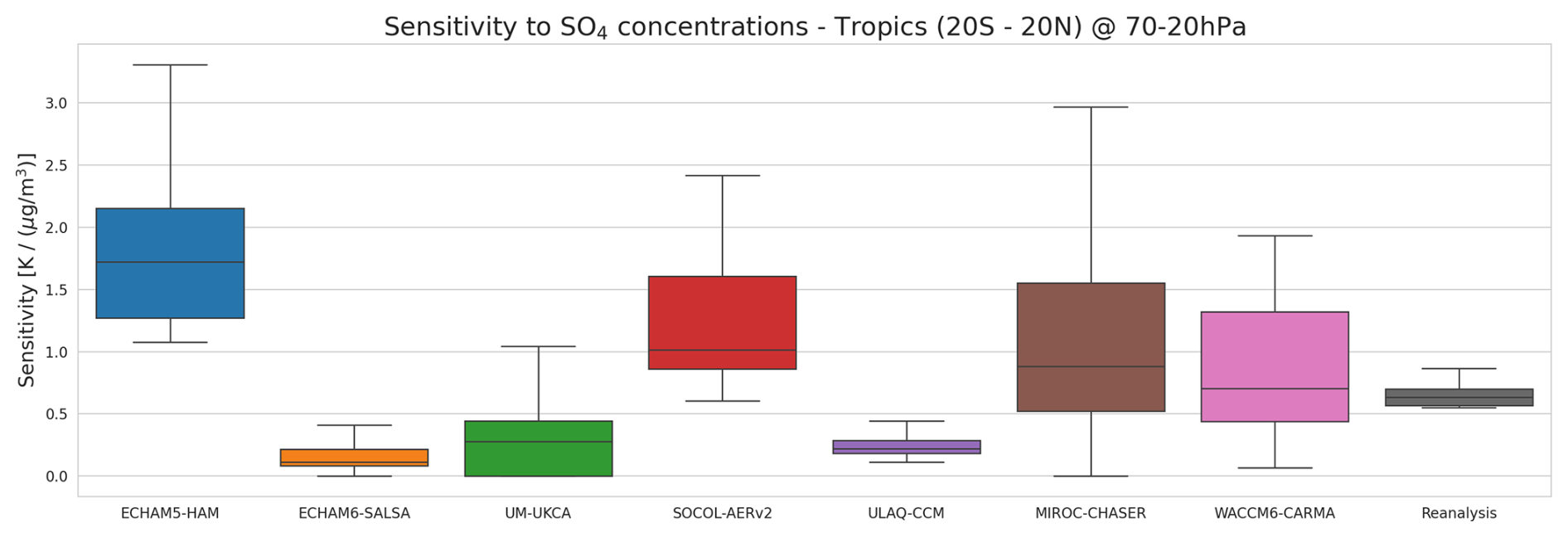
Figure 5Stratospheric temperature sensitivity to SO4 absorptive-heating of the ISA-MIP models and reanalysis in the tropics (20° S–20° N) between 70 and 20 hPa. The boxplots contain data for altitude weighted longitude – latitude pairs, obtained by regressing temperature anomalies against SO4 concentrations over time.
3.5 Comparison to other Multi-model Intercomparison Projects
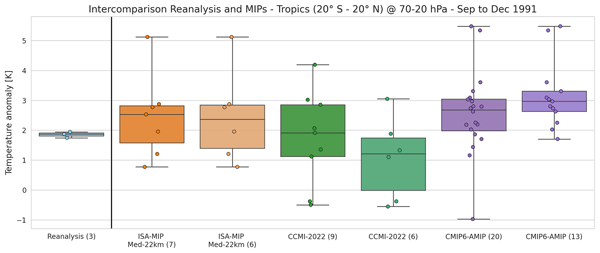
These results show that even when following a strict simulation protocol, as put forward by ISA-MIP HErSEA, model outcomes for aerosol concentration and subsequent temperature change in the middle and lower stratosphere differ widely. Some of these model differences may be attributed to the use of specific aerosol schemes and/or interactive chemistry in some of the models (see Table 1). Thus, we expect that the inter-model spread can be reduced if even stricter protocols are applied. We test this hypothesis through recent MIPs under the auspices of the World Climate Research Programme (WCRP) that use prescribed SADs: CCMI-2022 REF-D1 and CMIP6-AMIP. While for the ISA-MIP models a Control run without the Mt. Pinatubo eruption is available and used for computing forced anomalies, no such Control is available for CCMI-2022 and CMIP6-AMIP. Thus, for these two MIPs, and also for the reanalyses in this comparison, we compute anomalies with respect to the mean of the period 1980–2000 (21 years centred around the Mt. Pinatubo eruption). We note in passing, that such anomaly calculation yields only a slightly broader range of anomalies for the reanalysis than the MLR calculation used above (see Fig. A1), which is, however, still substantially narrower than for the ISA-MIP models, see Fig. 6. We focus on the time period, latitude band and pressure range in which the strongest signal in observations is found (September to December 1991, 20° S–20° N, 70 to 20 hPa).
As in our MLR analysis, we find that the temperature anomalies derived for ERA5, MERRA2, and JRA55 agree well with each other and also show a similar spread for the selected period and vertical range (see Fig. 6). Our analysis also shows that the median/mean of the multi-model temperature anomaly agrees well with reanalyses for all MIPs considered, while the distribution of the temperature anomaly is much wider for MIPs than for reanalyses, indicating that the agreement in the median/mean occurs through error compensation when averaging across models.
For CCMI-2022 we find a slightly lower magnitude of temperature anomaly compared to ISA-MIP, but a median still in close agreement with reanalyses. More interestingly, however, the intra-ensemble spread (evaluated from minimum to maximum values) in CCMI-2022 is even increased (longer whiskers, wider box) compared to ISA-MIP. We interpret this outcome as follows: model complexity (i.e. inclusion/absence of interactive aerosol microphysical schemes) appears to be of secondary importance compared to other factors such as the radiative transfer scheme or model selection. Expansion of this analysis to CMIP6-AMIP further supports this interpretation as for these models the intra-model spread is even larger (longer whiskers, narrower box) while the median is marginally larger than for ISA-MIP models or reanalyses. The hypothesis that there is strong model-dependency of the temperature anomalies obtained is further supported when for the same comparison only models with more than one ensemble member are taken into account (see light orange, light green and light purple boxplots in Fig. 6, respectively). On the one hand, an increase or decrease in the multi-model median is found for individual MIPs when subset, on the other, also the intra-model spread is altered. For convenient reference we indicate individual models with dots per MIP (and subset), which further corroborates the sensitivity to model selection as visual inspection clearly shows that selecting or excluding a model (or subset of models) would strongly affect the overall result.
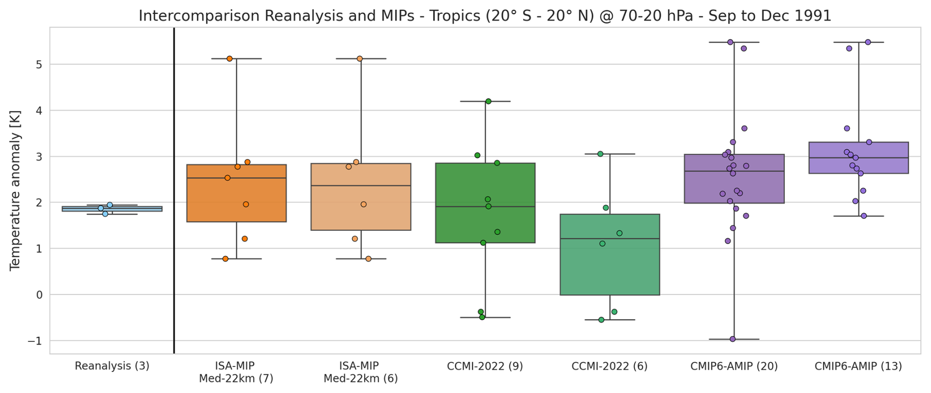
Figure 6Temperature anomaly distributions for reanalyses (left), ISA-MIP and CCMI-2022 (center) and CMIP6-AMIP (right) in the tropics (20° S–20° N) averaged between 70 and 20 hPa in the period September to December 1991. The number in brackets indicates the number of models used. Solid vertical line separates reanalysis from models. Light orange, light green and light purple boxplots represent models with more than one ensemble member. Individual model results are provided as dots in the same colour of the corresponding MIP/sample. For convenient reference we note the order of ISA-MIP models in descending temperature anomaly: SOCOL-AERv2, ECHAM5-HAM, WACCM6-CARMA, ULAQ-CCM, UM-UKCA, ECHAM6-SALSA, MIROC-CHASER.
Here we use the well-defined experimental protocol of the ISA-MIP HErSEA experiments to investigate the stratospheric temperature response to the Mt. Pinatubo eruption of 1991. To this end, we compare outputs of a group of climate models with interactive stratospheric aerosol microphysics to observations and reanalysis. We explicitly focus on the evolution of the temperature response to changes in SO4 concentration to highlight similarities and differences across the models under uniform conditions for volcanic SO2 injection in magnitude and altitude. We find that the multi-model mean of stratospheric temperature anomalies agrees well with the reanalysis mean for these experiments (±1 K in the first four months after the eruption, see Fig. 1). Individual ISA-MIP HErSEA experiments differ in injection amount and altitude. Overall, the model results confirm our understanding of stratospheric aerosol forcing, i.e. that larger injection of SO2 leads to a stronger warming response. Injection at a lower altitude leads to faster removal of the volcanic aerosols from the stratosphere and therefore a shorter duration of the temperature signal compared to reanalysis. While these physical relationships are present in most of the models, substantial spread in magnitude and duration of the temperature response is apparent, a result somewhat surprising given the strict experimental protocol. We find that differences between the models are in most cases larger than differences in the individual models across experiments. Therefore, our results highlight that the representation of transport, radiative transfer and microphysics, as well as the treatment/characterization of aerosol size distributions, plays a crucial role in the emergence of the widespread simulated temperature response. Since these processes interact with one another, it is not trivial to extract the exact reason of the differences among models. Below, we discuss the role of transport, radiation scheme, and the usage of interactive aerosol models and aerosol size distribution.
We first analysed the evolution of the mass concentration of SO4 resulting from the volcanic plume, which acts as a tracer for transport affected only by formation and removal processes, and simultaneously represents the LW forcing for particles of an effective radius smaller than approximately 0.5 µm. All models following the ISA-MIP HErSEA protocol show a transport bias, i.e. preferred transport into the NH, which is in disagreement with REMAP-GloSSAC-2023 observations. This is in agreement with the findings of Quaglia et al. (2023), who relate the transport bias on the one hand to the point-injection strategy (compare also in our manuscript Figs. 2 and A3) and on the other to the absence of the Cerro Hudson eruption of August 1991 in the ISA-MIP HErSEA protocol. Such biases could be at least partially mitigated in future MIPs through application of a regional injection strategy (Tilmes et al., 2023), consideration of volcanic ash emissions alongside sulfur (Niemeier et al., 2009, 2021), and consideration of co-occurring volcanic events.
We also identified marked differences across models in SO4 concentration already in the first months after SO2 injection concerning the vertical spread of the SO4 plume, the rate of confinement in the tropical pipe vs. partial transport through the shallow branch of the BDC. We attribute these early differences to the combined effect of SO2 conversion rates, transport, model vertical velocity and resolution, in broad agreement with model differences identified in Niemeier et al. (2020). In the subsequent months, the models continue to differ in terms of the way of transport. While some models (e.g. EMAC, ECHAM6-SALSA, SOCOL-AERv2) show preferred transport through the shallow branch, others (e.g. UM-UKCA, WACCM6-CARMA, MIROC-CHASER) mainly transport through the deep branch. Similar differences in transport have also been highlighted in multi-model studies with a focus on age of air, in CMIP6 (Abalos et al., 2021) and CCMI-2020 (Eichinger et al., 2019). Furthermore, recent research revealed effects of QBO representation on transport (e.g., Zhuo et al., 2024). Following the experimental protocol, all models matched the observed post-Pinatubo QBO transition, either by nudging or from re-initialising from a prior control run. Given this uniform QBO treatment and the small effect on temperature anomalies in the models analysed (see Sect. 2.3.2 and Fig. A2), we do not consider it a prime contributor to overall model spread.
In addition, some differences in vertical transport/sedimentation are apparent in the models. Here, MIROC-CHASER is an outlier in the model set, with limited sedimentation and a non-apparent subtropical transport barrier. This might be to some extent explained by the models' low horizontal resolution (T42) and model top (∼ 50 km), although other low-resolution models such as SOCOL-AERv2 manage to represent the transport quite well. To analyse if the identified differences in transport dominate the model temperature response, we compared the co-alignment of the peaks in SO4 concentration and temperature anomaly. While at first order we find a good agreement between these peaks in the individual models, significant differences exist among the models in the magnitude of the temperature anomaly and, consequently, in their sensitivity to SO4 concentrations. These might be explained by differences in radiative transfer schemes (see Table 1) and furthermore differences in the particle size distribution (Quaglia et al., 2023).
Since for most of the models the effective radius is smaller or around 0.5µm (shown in Quaglia et al., 2023) in the first year after the eruption, we assume that absorption is not substantially affected by particle size. We note for completeness that ULAQ-CCM and WACCM6-CARMA have substantially larger effective radii at lower altitudes. Temperature anomalies in these layers differ, however, strongly between these two models, and as information on aerosol size distribution is not available beyond the effective radius, further interpretation remains unfeasible. Another exception is ECHAM6-SALSA which shows only a weak warming signal in our analysis. Such a dampened temperature signal for ECHAM6-SALSA was also identified by Laakso et al. (2022) in comparison to simulations performed with ECHAM6-M7. The authors attribute this dampening to the efficient formation of new particles occurring at the expense of gaseous sulfuric acid condensing onto pre-existing particles. Interestingly, however, the effective radius in ECHAM6-SALSA was found to be comparable to observations and the other models (Quaglia et al., 2023). Furthermore, transport and sedimentation also depend on particle size and substantial differences in the deposition of volcanic sulfur from the 1815 eruption of Mt. Tambora have been identified in Marshall et al. (2018). Recently Tilmes et al. (2026) highlighted in a study focusing on SAI sensitivity that the aerosol burden and mass distribution can vary significantly in the same modelling framework depending on the aerosol microphysical module used (sectional or modal), with implications for radiative forcing and impacts. Taken together, this shows that the simulated size distribution is somewhat important for a correct representation of the observed temperature response. Therefore, a detailed analysis of the size distributions of the models and the ability of the effective radius to represent them is suggested for future work. For now we consider this beyond the scope of the presented study given that for the bulk of the models effective radii do not seem to be a main contributor to the differences identified. Another candidate to explain the spread in temperature response in the ISA-MIP models, is the use of interactive aerosol schemes. To test this hypothesis we compared the ISA-MIP multi-model distribution with those obtained from CCMI-2022 and CMIP6-AMIP, which use prescribed SADs. If indeed interactive aerosol treatment would be a key contributor to model spread, one would expect to obtain narrower multi-model distributions from CCMI-2022 and CMIP6-AMIP. Interestingly, this hypothesis has to be rejected, as no reduction in the multi-model spread is found. One important point to note is that all MIPs considered comprise different model families. And, while the individual multi-model temperature anomalies agree quite well with those of reanalyses, our study shows that agreement in the median occurs through error compensation when averaging across models. The analysis and the sensitivity tests for model selection presented here highlight that by far the most important factor driving both magnitude and spread of the multi-model distribution in temperature response to volcanic aerosol forcing is model choice.
The results of our multi-model comparison argue for caution given the large spread in aerosol burden and transport and resulting stratospheric temperature response – even in the case of a strict experimental protocol. Even more so, given our present-day understanding of the role of aerosol-induced stratospheric warming for dynamics and chemistry and subsequently coupling across atmospheric layers and potentially surface climate.
Given the importance of progress in understanding the root cause of differences in model response to stratospheric (volcanic) aerosol forcing, some future directions can be informed from the results presented and limitations identified here: (i) implementation of strict experimental protocols to ensure a robust baseline for comparison, while understanding that this alone does not allow for a full attribution of similarities and differences across participating models. (ii) supplementing the core experimental protocol with process-oriented MIPs to individually address uncertainties in core components, such as radiative transfer, transport and sedimentation. (iii) sensitivity tests to identify the impact of changes in model subroutines affecting core variables for aerosol-climate connections to ensure robustness within model families and generations. (iv) more than one ensemble member per model simulation to quantify intra-model spread. (v) strict MIP protocol ensuring delivery of data variables necessary to support all items listed above.
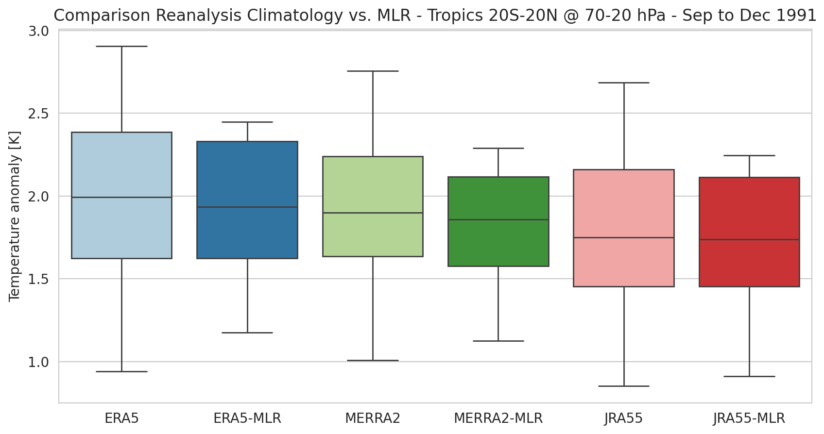
Figure A1Temperature anomaly distribution of reanalysis data before (bright colours) and after MLR (dark colours) in the tropics between 70 and 20 hPa in the period from September to December 1991. All calculations use 1980–2000 as the base period.
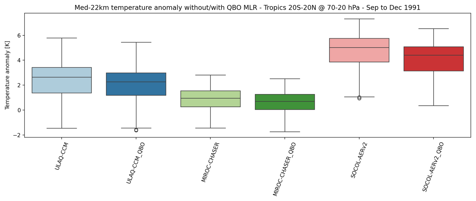
Figure A2Temperature anomalies in the Med-22km experiment for selected ISA-MIP models with QBO effects included or regressed out. For ULAQ-CCM, MIROC-CHASER and SOCOL-AERv2 temperature anomalies are derived by using the Control runs as reference. For ULAQ-CCM_QBO, MIROC-CHASER_QBO and SOCOL-AERv2_QBO the QBO signal was removed in experiment and Control, using the wind field at 30 and 50 hPa before anomalies were derived.
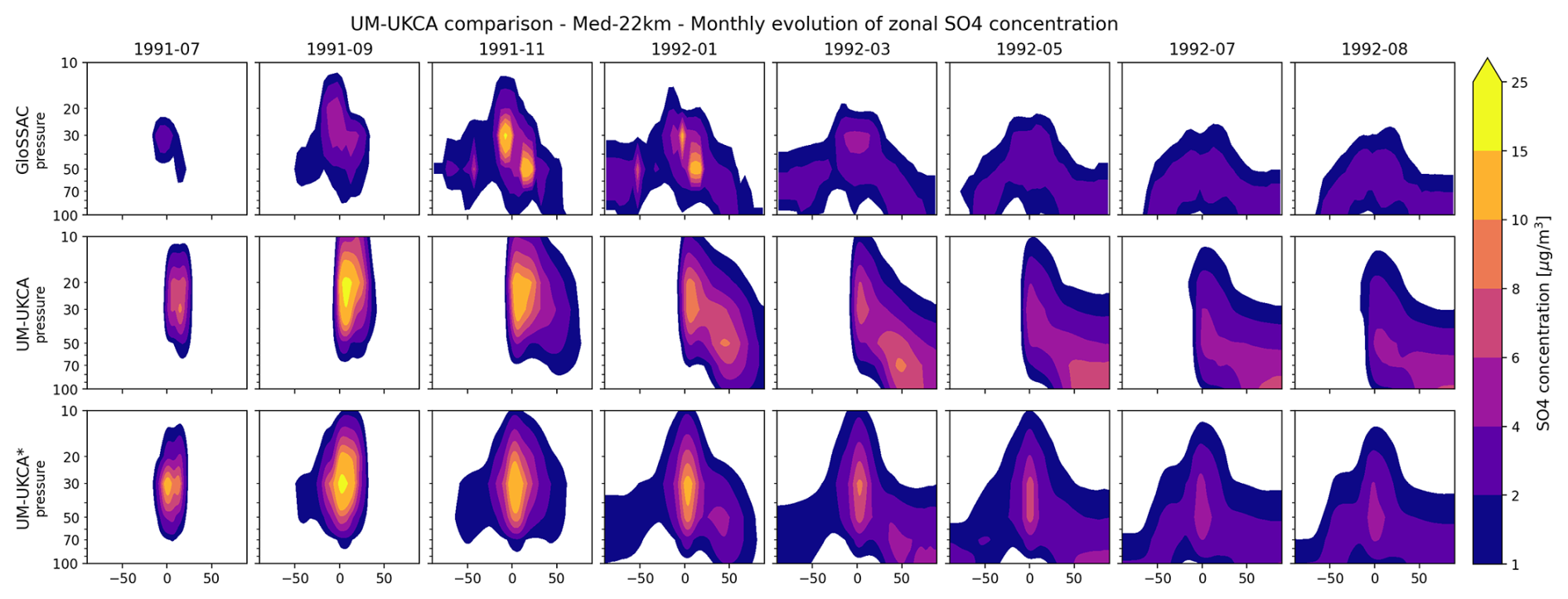
Figure A3Temperature anomalies in experiment Med-22km for UM-UKCA runs with different injection strategies. UM-UKCA uses the injection strategy as defined in the ISA-MIP HErSEA protocols (SO2 injection in a single grid cell close to the Mt. Pinatubo location (15° N, 120° E)) while in UM-UKCA* SO2 is injected at Mt. Pinatubo longitude in a latitude range between 0 and 15° N. REMAP-GloSSAC-2023 observations are provided for convenient reference in the top row.
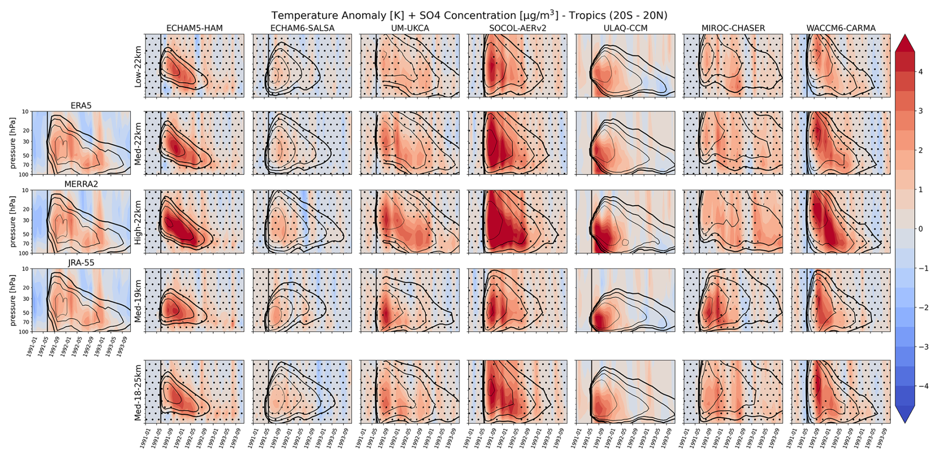
Figure A4Vertical time evolution of the temperature anomalies for all experiments and models in the tropics (20° S–20° N). In all panels: SO4 concentrations are shown as contours (levels are 0.5, 1, 2, 5 µg m−3), dots indicate non-significant areas (p-value > 0.05) for reanalysis and models with the exception of ULAQ-CCM where only one ensemble member is available, and the thick black vertical line represents the Mt. Pinatubo eruption time.
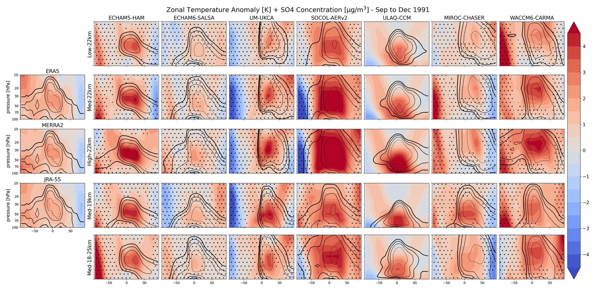
Figure A5Vertical zonal temperature anomaly for all experiments and models for the period September to December 1991. In all panels: SO4 concentrations are shown as contours (levels are 0.5, 1, 2, 5 µg m−3), dots indicate non-significant areas (p-value >0.05) for reanalysis and models with the exception of ULAQ-CCM where only one ensemble member is available, and the vertical lines embed the tropical region (20° S–20° N).
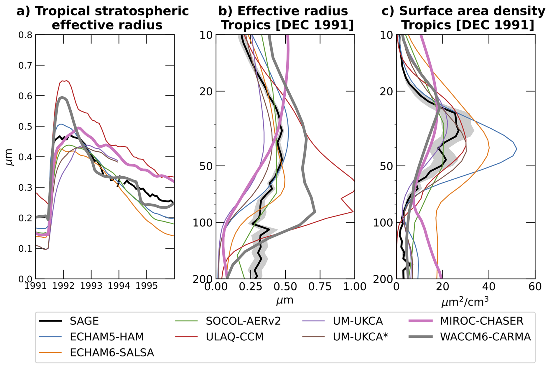
Figure A6Vertical profile of effective radius (a) and time evolution of stratospheric effective radius (µm) (b) in the tropics for Med-22km. Model results are compared to SAGE II following Quaglia et al. (2023).
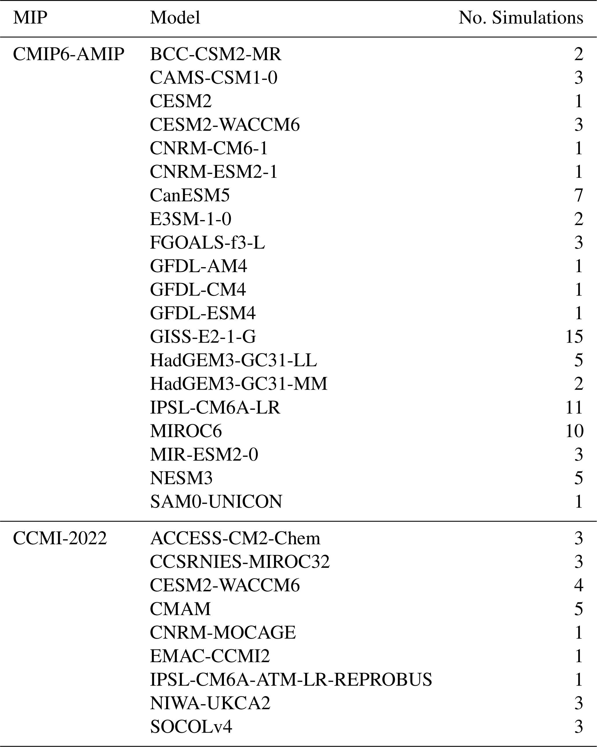
Table A2RMSE for the time evolution of the observed (multi-reanalysis mean) and model-derived tropical mean temperature anomaly normalized to June 1991 for different pressure levels for individual models.
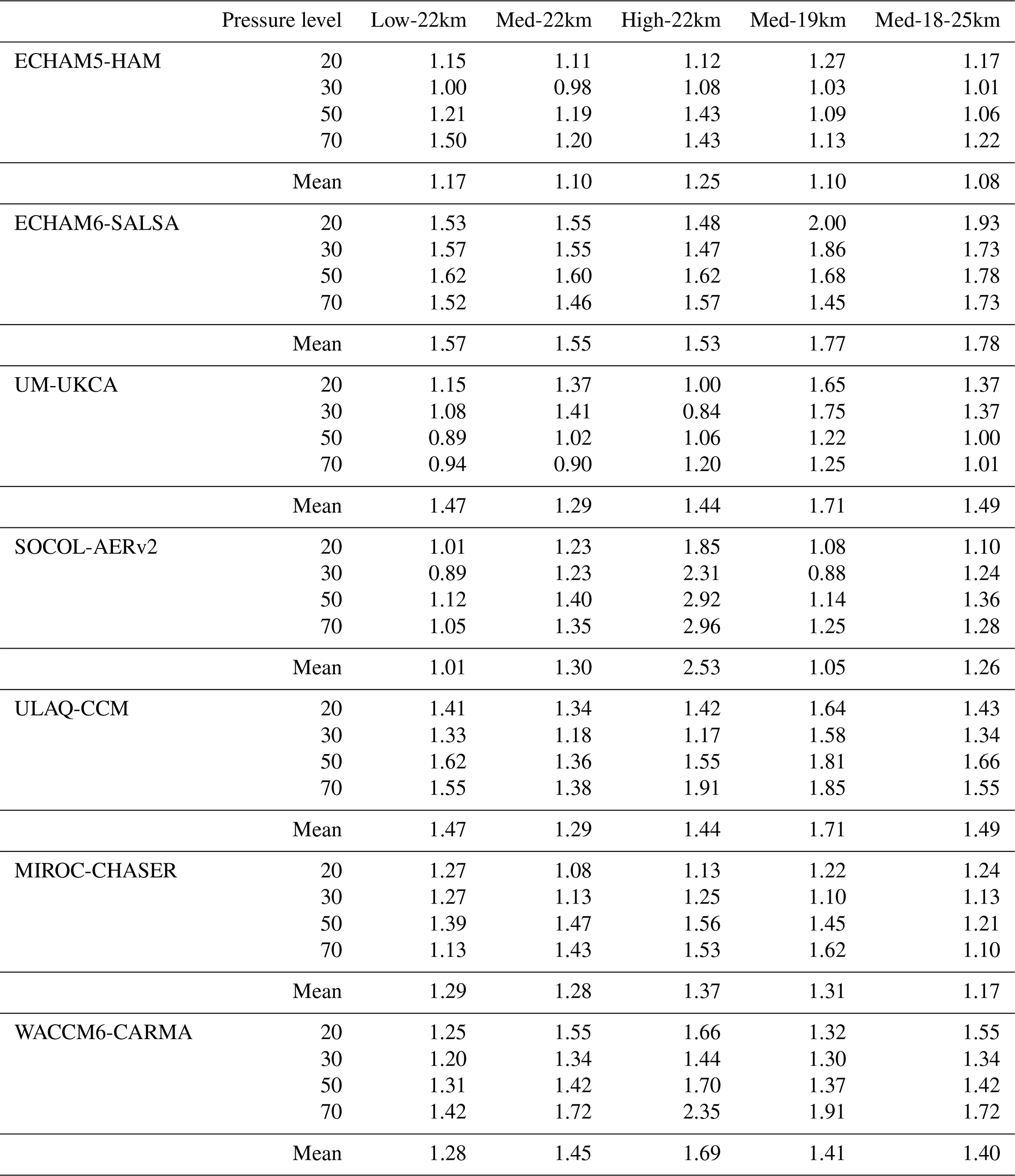
Reanalysis data (MERRA2, ERA5, JRA55) are available from https://doi.org/10.5285/B241A7F536A244749662360BD7839312 (Martineau, 2017). REMAP-GloSSAC-2023 data are available from https://doi.org/10.3929/ethz-b-000713396 (Jörimann, 2025). CCMI-2022 data are available from https://data.ceda.ac.uk/badc/ccmi/data/post-cmip6/ccmi-2022 (last access: 29 August 2025) and CMIP6-AMIP data was accessed on DATE from https://registry.opendata.aws/cmip6 (last access: 3 July 2025). ISA-MIP HErSEA outputs are available from model PIs. Aggregated datasets produced in this study and code to reproduce the figures of this article are available from KP upon request.
KP, TS, AK, PA and HR designed the analysis. AK prepared data from reanalyses and AJ prepared REMAP-GloSSAC-2023. KP lead the study, performed all analyses and visualizations and wrote the initial draft of the paper. All authors contributed to the discussion and finalization of the article. The authors thank Matthew Toohey for his constructive feedback on an earlier version of this manuscript.
At least one of the (co-)authors is a member of the editorial board of Atmospheric Chemistry and Physics. The peer-review process was guided by an independent editor, and the authors also have no other competing interests to declare.
Publisher's note: Copernicus Publications remains neutral with regard to jurisdictional claims made in the text, published maps, institutional affiliations, or any other geographical representation in this paper. The authors bear the ultimate responsibility for providing appropriate place names. Views expressed in the text are those of the authors and do not necessarily reflect the views of the publisher.
The paper is part of the “Interactive Model Intercomparison Project” from the WCRP/SPARC activity “Stratospheric Sulfur and its Role in Climate” (SSiRC). SSD was supported by the UK Natural Environment Research Council (NERC) through the projects UKESM (NE/N017951/1) and TerraFIRMA (NE/W004895/1). UN and CT were supported by the Deutsche Forschungsgemeinschaft (DFG) Research Unit VollImpact (FOR2820, grant no. 398006378) and use resources of the Deutsches Klimarechenzentrum (DKRZ) granted by its Scientific Steering Committee (WLA) under project ID bm855 “ISA-MIP”. AJ acknowledges support from the Swiss National Science Foundation (SNSF) project AEON (grant no. 200020E_219166). KP acknowledges support by BOKU University. TS and KS were supported by MEXT-Program for the advanced studies of climate change projection (SENTAN) Grant Number JPMXD0722681344. IQ and ST acknowledge support from the US Simons Foundation (grant ref. MPS-SRM-00005203) and the National Center for Atmospheric Research, which is a major facility sponsored by the NSF under Cooperative Agreement No. 1852977. ST acknowledges support from the NOAA Climate Program Office Earth's Radiation Budget Awards Number 03-01-07-001 and NA22OAR4310477. This work used resources of the high-performance computing support from the Derecho system (https://doi.org/10.5065/qx9a-pg09, Computational and Information Systems Laboratory, 2023).
This research has been supported by the Natural Environment Research Council (grant nos. NE/N017951/1 and NE/W004895/1), the Deutsche Forschungsgemeinschaft (grant no. 398006378), the Deutsches Klimarechenzentrum (grant no. bm855 “ISA-MIP”), the Ministry of Education, Culture, Sports, Science and Technology (grant no. JPMXD0722681344), the Simons Foundation (grant no. MPS-SRM-00005203), and the Schweizerischer Nationalfonds zur Förderung der Wissenschaftlichen Forschung (grant no. 200020E_219166).
This paper was edited by Kostas Tsigaridis and reviewed by two anonymous referees.
Abalos, M., Calvo, N., Benito-Barca, S., Garny, H., Hardiman, S. C., Lin, P., Andrews, M. B., Butchart, N., Garcia, R., Orbe, C., Saint-Martin, D., Watanabe, S., and Yoshida, K.: The Brewer–Dobson circulation in CMIP6, Atmos. Chem. Phys., 21, 13571–13591, https://doi.org/10.5194/acp-21-13571-2021, 2021. a
Abdelkader, M., Stenchikov, G., Pozzer, A., Tost, H., and Lelieveld, J.: The effect of ash, water vapor, and heterogeneous chemistry on the evolution of a Pinatubo-size volcanic cloud, Atmos. Chem. Phys., 23, 471–500, https://doi.org/10.5194/acp-23-471-2023, 2023. a
Alam, M.: The effect of van der Waals and viscous forces on aerosol coagulation, Aerosol Sci. Technol., 41–52, https://doi.org/10.1080/02786828708959118, 1987. a
Antuña, J. C., Robock, A., Stenchikov, G. L., Thomason, L. W., and Barnes, J. E.: Lidar validation of SAGE II aerosol measurements after the 1991 Mount Pinatubo eruption, J. Geophys. Res.-Atmos., 107, ACL 3–1–ACL 3–11, https://doi.org/10.1029/2001JD001441, 2002. a
Aquila, V., Oman, L. D., Stolarski, R., Douglass, A. R., and Newman, P. A.: The Response of Ozone and Nitrogen Dioxide to the Eruption of Mt. Pinatubo at Southern and Northern Midlatitudes, J. Atmos. Sci., 70, 894–900, https://doi.org/10.1175/JAS-D-12-0143.1, 2013. a
Aquila, V., Garfinkel, C. I., Newman, P., Oman, L., and Waugh, D.: Modifications of the quasi-biennial oscillation by a geoengineering perturbation of the stratospheric aerosol layer, Geophys. Res. Lett., 41, 1738–1744, https://doi.org/10.1002/2013GL058818, 2014. a
Archibald, A. T., O'Connor, F. M., Abraham, N. L., Archer-Nicholls, S., Chipperfield, M. P., Dalvi, M., Folberth, G. A., Dennison, F., Dhomse, S. S., Griffiths, P. T., Hardacre, C., Hewitt, A. J., Hill, R. S., Johnson, C. E., Keeble, J., Köhler, M. O., Morgenstern, O., Mulcahy, J. P., Ordóñez, C., Pope, R. J., Rumbold, S. T., Russo, M. R., Savage, N. H., Sellar, A., Stringer, M., Turnock, S. T., Wild, O., and Zeng, G.: Description and evaluation of the UKCA stratosphere–troposphere chemistry scheme (StratTrop vn 1.0) implemented in UKESM1, Geosci. Model Dev., 13, 1223–1266, https://doi.org/10.5194/gmd-13-1223-2020, 2020. a
Barnes, E. A., Solomon, S., and Polvani, L. M.: Robust Wind and Precipitation Responses to the Mount Pinatubo Eruption, as Simulated in the CMIP5 Models, J. Climate, 29, 4763–4778, https://doi.org/10.1175/JCLI-D-15-0658.1, 2016. a
Benito-Barca, S., Abalos, M., Calvo, N., Garny, H., Birner, T., Abraham, N. L., Akiyoshi, H., Dennison, F., Jöckel, P., Josse, B., Keeble, J., Kinnison, D., Marchand, M., Morgenstern, O., Plummer, D., Rozanov, E., Strode, S., Sukhodolov, T., Watanabe, S., and Yamashita, Y.: Recent Lower Stratospheric Ozone Trends in CCMI-2022 Models: Role of Natural Variability and Transport, J. Geophys. Res.-Atmos., 130, e2024JD042412, https://doi.org/10.1029/2024JD042412, 2025. a
Boretti, A.: Reassessing the cooling that followed the 1991 volcanic eruption of Mt. Pinatubo, J. Atmos. Sol.-Terr. Phys., 256, 106187, https://doi.org/10.1016/j.jastp.2024.106187, 2024. a
Borrmann, S., Dye, J. E., Baumgardner, D., Proffitt, M. H., Margitan, J. J., Wilson, J. C., Jonsson, H. H., Brock, C. A., Loewenstein, M., Podolske, J. R., and Ferry, G. V.: Aerosols as dynamical tracers in the lower stratosphere: Ozone versus aerosol correlation after the Mount Pinatubo eruption, J. Geophys. Res.-Atmos., 100, 11147–11156, https://doi.org/10.1029/95JD00016, 1995. a
Brodowsky, C. V., Sukhodolov, T., Chiodo, G., Aquila, V., Bekki, S., Dhomse, S. S., Höpfner, M., Laakso, A., Mann, G. W., Niemeier, U., Pitari, G., Quaglia, I., Rozanov, E., Schmidt, A., Sekiya, T., Tilmes, S., Timmreck, C., Vattioni, S., Visioni, D., Yu, P., Zhu, Y., and Peter, T.: Analysis of the global atmospheric background sulfur budget in a multi-model framework, Atmos. Chem. Phys., 24, 5513–5548, https://doi.org/10.5194/acp-24-5513-2024, 2024. a
Brooke, J. S. A., Feng, W., Carrillo-Sánchez, J. D., Mann, G. W., James, A. D., Bardeen, C. G., Marshall, L., Dhomse, S. S., and Plane, J. M. C.: Meteoric Smoke Deposition in the Polar Regions: A Comparison of Measurements With Global Atmospheric Models, J. Geophys. Res.-Atmos., 122, 11112–11130, https://doi.org/10.1002/2017JD027143, 2017. a
Brühl, C., Schallock, J., and Diehl, T.: Volcanic SO2 data derived from limb viewing satellites for the lower stratosphere from 1990 to 2019, and from nadir viewing satellites for the troposphere, including the corresponding radiative forcing computed by the CCM EMAC, World Data Center for Climate (WDCC) at DKRZ [data set], https://doi.org/10.26050/WDCC/SSIRC_3, 2021. a
Clyne, M., Lamarque, J.-F., Mills, M. J., Khodri, M., Ball, W., Bekki, S., Dhomse, S. S., Lebas, N., Mann, G., Marshall, L., Niemeier, U., Poulain, V., Robock, A., Rozanov, E., Schmidt, A., Stenke, A., Sukhodolov, T., Timmreck, C., Toohey, M., Tummon, F., Zanchettin, D., Zhu, Y., and Toon, O. B.: Model physics and chemistry causing intermodel disagreement within the VolMIP-Tambora Interactive Stratospheric Aerosol ensemble, Atmos. Chem. Phys., 21, 3317–3343, https://doi.org/10.5194/acp-21-3317-2021, 2021. a
Colella, P. and Woodward, P. R.: The Piecewise Parabolic Method (PPM) for gas-dynamical simulations, J. Comput. Phys., 54, 174–201, https://doi.org/10.1016/0021-9991(84)90143-8, 1984. a
Collins, W. J., Bellouin, N., Doutriaux-Boucher, M., Gedney, N., Halloran, P., Hinton, T., Hughes, J., Jones, C. D., Joshi, M., Liddicoat, S., Martin, G., O'Connor, F., Rae, J., Senior, C., Sitch, S., Totterdell, I., Wiltshire, A., and Woodward, S.: Development and evaluation of an Earth-System model – HadGEM2, Geosci. Model Dev., 4, 1051–1075, https://doi.org/10.5194/gmd-4-1051-2011, 2011. a
Computational and Information Systems Laboratory: Derecho: HPE Cray EX System (NCAR Community Computing), Boulder, CO, National Center for Atmospheric Research, https://doi.org/10.5065/qx9a-pg09, 2023. a
Crutzen, P. J.: Albedo Enhancement by Stratospheric Sulfur Injections: A Contribution to Resolve a Policy Dilemma?, Climatic Change, 77, 211–220, https://doi.org/10.1007/s10584-006-9101-y, 2006. a
DallaSanta, K., Gerber, E. P., and Toohey, M.: The Circulation Response to Volcanic Eruptions: The Key Roles of Stratospheric Warming and Eddy Interactions, J.f Climate, 32, 1101–1120, https://doi.org/10.1175/JCLI-D-18-0099.1, 2019. a
Danabasoglu, G., Lamarque, J.-F., Bacmeister, J., Bailey, D. A., DuVivier, A. K., Edwards, J., Emmons, L. K., Fasullo, J., Garcia, R., Gettelman, A., Hannay, C., Holland, M. M., Large, W. G., Lauritzen, P. H., Lawrence, D. M., Lenaerts, J. T. M., Lindsay, K., Lipscomb, W. H., Mills, M. J., Neale, R., Oleson, K. W., Otto-Bliesner, B., Phillips, A. S., Sacks, W., Tilmes, S., van Kampenhout, L., Vertenstein, M., Bertini, A., Dennis, J., Deser, C., Fischer, C., Fox-Kemper, B., Kay, J. E., Kinnison, D., Kushner, P. J., Larson, V. E., Long, M. C., Mickelson, S., Moore, J. K., Nienhouse, E., Polvani, L., Rasch, P. J., and Strand, W. G.: The Community Earth System Model Version 2 (CESM2), J. Adv. Model. Earth Sy., 12, e2019MS001916, https://doi.org/10.1029/2019MS001916, 2020. a
Davies, T., Cullen, M. J. P., Malcolm, A. J., Mawson, M. H., Staniforth, A., White, A. A., and Wood, N.: A new dynamical core for the Met Office's global and regional modelling of the atmosphere, Q. J. Roy. Meteo. Soc., 131, 1759–1782, https://doi.org/10.1256/qj.04.101, 2005. a
Davis, N. A., Visioni, D., Garcia, R. R., Kinnison, D. E., Marsh, D. R., Mills, M., Richter, J. H., Tilmes, S., Bardeen, C. G., Gettelman, A., Glanville, A. A., MacMartin, D. G., Smith, A. K., and Vitt, F.: Climate, Variability, and Climate Sensitivity of “Middle Atmosphere” Chemistry Configurations of the Community Earth System Model Version 2, Whole Atmosphere Community Climate Model Version 6 (CESM2(WACCM6)), J. Adv. Model. Earth Sy., 15, e2022MS003579, https://doi.org/10.1029/2022MS003579, 2023. a, b
Dee, D. P., Uppala, S. M., Simmons, A. J., Berrisford, P., Poli, P., Kobayashi, S., Andrae, U., Balmaseda, M. A., Balsamo, G., Bauer, P., Bechtold, P., Beljaars, A. C. M., van de Berg, L., Bidlot, J., Bormann, N., Delsol, C., Dragani, R., Fuentes, M., Geer, A. J., Haimberger, L., Healy, S. B., Hersbach, H., Hólm, E. V., Isaksen, L., Kållberg, P., Köhler, M., Matricardi, M., McNally, A. P., Monge-Sanz, B. M., Morcrette, J.-J., Park, B.-K., Peubey, C., de Rosnay, P., Tavolato, C., Thépaut, J.-N., and Vitart, F.: The ERA-Interim reanalysis: configuration and performance of the data assimilation system, Q. J. Roy. Meteor. Soc., 137, 553–597, https://doi.org/10.1002/qj.828, 2011. a
Deshler, T., Hervig, M. E., Hofmann, D. J., Rosen, J. M., and Liley, J. B.: Thirty years of in situ stratospheric aerosol size distribution measurements from Laramie, Wyoming (41°N), using balloon-borne instruments, J. Geophys. Res.-Atmos., 108, https://doi.org/10.1029/2002JD002514, 2003. a
Dhomse, S. S., Emmerson, K. M., Mann, G. W., Bellouin, N., Carslaw, K. S., Chipperfield, M. P., Hommel, R., Abraham, N. L., Telford, P., Braesicke, P., Dalvi, M., Johnson, C. E., O'Connor, F., Morgenstern, O., Pyle, J. A., Deshler, T., Zawodny, J. M., and Thomason, L. W.: Aerosol microphysics simulations of the Mt. Pinatubo eruption with the UM-UKCA composition-climate model, Atmos. Chem. Phys., 14, 11221–11246, https://doi.org/10.5194/acp-14-11221-2014, 2014. a
Dhomse, S. S., Chipperfield, M. P., Feng, W., Hossaini, R., Mann, G. W., and Santee, M. L.: Revisiting the hemispheric asymmetry in midlatitude ozone changes following the Mount Pinatubo eruption: A 3-D model study, Geophys. Res. Lett., 42, 3038–3047, https://doi.org/10.1002/2015GL063052, 2015. a
Dhomse, S. S., Mann, G. W., Antuña Marrero, J. C., Shallcross, S. E., Chipperfield, M. P., Carslaw, K. S., Marshall, L., Abraham, N. L., and Johnson, C. E.: Evaluating the simulated radiative forcings, aerosol properties, and stratospheric warmings from the 1963 Mt Agung, 1982 El Chichón, and 1991 Mt Pinatubo volcanic aerosol clouds, Atmos. Chem. Phys., 20, 13627–13654, https://doi.org/10.5194/acp-20-13627-2020, 2020. a, b, c, d
Diallo, M., Ploeger, F., Konopka, P., Birner, T., Müller, R., Riese, M., Garny, H., Legras, B., Ray, E., Berthet, G., and Jegou, F.: Significant Contributions of Volcanic Aerosols to Decadal Changes in the Stratospheric Circulation, Geophys. Res. Lett., 44, 10780–10791, https://doi.org/10.1002/2017GL074662, 2017. a
Driscoll, S., Bozzo, A., Gray, L. J., Robock, A., and Stenchikov, G.: Coupled Model Intercomparison Project 5 (CMIP5) simulations of climate following volcanic eruptions, J. Geophys. Res.-Atmos., 117, https://doi.org/10.1029/2012JD017607, 2012. a
Dutton, E. G. and Christy, J. R.: Solar radiative forcing at selected locations and evidence for global lower tropospheric cooling following the eruptions of El Chichón and Pinatubo, Geophys. Res. Lett., 19, 2313–2316, https://doi.org/10.1029/92GL02495, 1992. a
Eichinger, R., Dietmüller, S., Garny, H., Šácha, P., Birner, T., Bönisch, H., Pitari, G., Visioni, D., Stenke, A., Rozanov, E., Revell, L., Plummer, D. A., Jöckel, P., Oman, L., Deushi, M., Kinnison, D. E., Garcia, R., Morgenstern, O., Zeng, G., Stone, K. A., and Schofield, R.: The influence of mixing on the stratospheric age of air changes in the 21st century, Atmos. Chem. Phys., 19, 921–940, https://doi.org/10.5194/acp-19-921-2019, 2019. a
Eyring, V., Bony, S., Meehl, G. A., Senior, C. A., Stevens, B., Stouffer, R. J., and Taylor, K. E.: Overview of the Coupled Model Intercomparison Project Phase 6 (CMIP6) experimental design and organization, Geosci. Model Dev., 9, 1937–1958, https://doi.org/10.5194/gmd-9-1937-2016, 2016. a
Feinberg, A., Sukhodolov, T., Luo, B.-P., Rozanov, E., Winkel, L. H. E., Peter, T., and Stenke, A.: Improved tropospheric and stratospheric sulfur cycle in the aerosol–chemistry–climate model SOCOL-AERv2, Geosci. Model Dev., 12, 3863–3887, https://doi.org/10.5194/gmd-12-3863-2019, 2019. a
Fouquart, Y. and Bonnel, B.: Computations of Solar Heating of the Earth’s Atmosphere – A New Parameterization, Beiträge zur Physik der Atmosphäre, 35–62, 1980. a
Fujiwara, M., Hibino, T., Mehta, S. K., Gray, L., Mitchell, D., and Anstey, J.: Global temperature response to the major volcanic eruptions in multiple reanalysis data sets, Atmos. Chem. Phys., 15, 13507–13518, https://doi.org/10.5194/acp-15-13507-2015, 2015. a, b
Gelaro, R., McCarty, W., Suárez, M. J., Todling, R., Molod, A., Takacs, L., Randles, C. A., Darmenov, A., Bosilovich, M. G., Reichle, R., Wargan, K., Coy, L., Cullather, R., Draper, C., Akella, S., Buchard, V., Conaty, A., Silva, A. M. d., Gu, W., Kim, G.-K., Koster, R., Lucchesi, R., Merkova, D., Nielsen, J. E., Partyka, G., Pawson, S., Putman, W., Rienecker, M., Schubert, S. D., Sienkiewicz, M., and Zhao, B.: The Modern-Era Retrospective Analysis for Research and Applications, Version 2 (MERRA-2), J. Climate, 30, 5419–5454, https://doi.org/10.1175/JCLI-D-16-0758.1, 2017. a
Gettelman, A., Mills, M. J., Kinnison, D. E., Garcia, R. R., Smith, A. K., Marsh, D. R., Tilmes, S., Vitt, F., Bardeen, C. G., McInerny, J., Liu, H.-L., Solomon, S. C., Polvani, L. M., Emmons, L. K., Lamarque, J.-F., Richter, J. H., Glanville, A. S., Bacmeister, J. T., Phillips, A. S., Neale, R. B., Simpson, I. R., DuVivier, A. K., Hodzic, A., and Randel, W. J.: The Whole Atmosphere Community Climate Model Version 6 (WACCM6), J. Geophys. Res.-Atmos., 124, 12380–12403, https://doi.org/10.1029/2019JD030943, 2019. a
Giorgetta, M. A. and Bengtsson, L.: Potential role of the quasi-biennial oscillation in the stratosphere-troposphere exchange as found in water vapor in general circulation model experiments, J. Geophys. Res.-Atmos., 104, 6003–6019, https://doi.org/10.1029/1998JD200112, 1999. a
Giorgetta, M. A., Manzini, E., Roeckner, E., Esch, M., and Bengtsson, L.: Climatology and Forcing of the Quasi-Biennial Oscillation in the MAECHAM5 Model, J. Climate, 19, 3882–3901, https://doi.org/10.1175/JCLI3830.1, 2006. a
Good, P. and Pyle, J.: Refinements in the use of equivalent latitude for assimilating sporadic inhomogeneous stratospheric tracer observations, 1: Detecting transport of Pinatubo aerosol across a strong vortex edge, Atmos. Chem. Phys., 4, 1823–1836, https://doi.org/10.5194/acp-4-1823-2004, 2004. a
Haywood, J. M., Boucher, O., Lennard, C., Storelvmo, T., Tilmes, S., and Visioni, D.: World Climate Research Programme lighthouse activity: an assessment of major research gaps in solar radiation modification research, Front. Climate, 7, https://doi.org/10.3389/fclim.2025.1507479, 2025. a
Hersbach, H., Bell, B., Berrisford, P., Hirahara, S., Horányi, A., Muñoz-Sabater, J., Nicolas, J., Peubey, C., Radu, R., Schepers, D., Simmons, A., Soci, C., Abdalla, S., Abellan, X., Balsamo, G., Bechtold, P., Biavati, G., Bidlot, J., Bonavita, M., De Chiara, G., Dahlgren, P., Dee, D., Diamantakis, M., Dragani, R., Flemming, J., Forbes, R., Fuentes, M., Geer, A., Haimberger, L., Healy, S., Hogan, R. J., Hólm, E., Janisková, M., Keeley, S., Laloyaux, P., Lopez, P., Lupu, C., Radnoti, G., de Rosnay, P., Rozum, I., Vamborg, F., Villaume, S., and Thépaut, J.-N.: The ERA5 global reanalysis, Q. J. Roy. Meteor. Soc., 146, 1999–2049, https://doi.org/10.1002/qj.3803, , 2020. a
Hommel, R., Timmreck, C., and Graf, H. F.: The global middle-atmosphere aerosol model MAECHAM5-SAM2: comparison with satellite and in-situ observations, Geosci. Model Dev., 4, 809–834, https://doi.org/10.5194/gmd-4-809-2011, 2011. a
Hurrell, J. W., Hack, J. J., Shea, D., Caron, J. M., and Rosinski, J.: A New Sea Surface Temperature and Sea Ice Boundary Dataset for the Community Atmosphere Model, J. Climate, 21, 5145–5153, https://doi.org/10.1175/2008JCLI2292.1, 2008. a
Huynh, H. N. and McNeill, V. F.: The potential environmental and climate impacts of stratospheric aerosol injection: a review, Environ. Sci. Atmos., 4, 114–143, https://doi.org/10.1039/D3EA00134B, 2024. a
Jöckel, P., Kerkweg, A., Pozzer, A., Sander, R., Tost, H., Riede, H., Baumgaertner, A., Gromov, S., and Kern, B.: Development cycle 2 of the Modular Earth Submodel System (MESSy2), Geosci. Model Dev., 3, 717–752, https://doi.org/10.5194/gmd-3-717-2010, 2010. a
Jörimann, A.: REMAP-GloSSAC-2023, ETH Zurich [data set], https://doi.org/10.3929/ethz-b-000713396, 2025. a
Jörimann, A., Sukhodolov, T., Luo, B., Chiodo, G., Mann, G., and Peter, T.: REtrieval Method for optical and physical Aerosol Properties in the stratosphere (REMAPv1), Geosci. Model Dev., 18, 6023–6041, https://doi.org/10.5194/gmd-18-6023-2025, 2025. a, b, c, d
Keeble, J., Hassler, B., Banerjee, A., Checa-Garcia, R., Chiodo, G., Davis, S., Eyring, V., Griffiths, P. T., Morgenstern, O., Nowack, P., Zeng, G., Zhang, J., Bodeker, G., Burrows, S., Cameron-Smith, P., Cugnet, D., Danek, C., Deushi, M., Horowitz, L. W., Kubin, A., Li, L., Lohmann, G., Michou, M., Mills, M. J., Nabat, P., Olivié, D., Park, S., Seland, Ø., Stoll, J., Wieners, K.-H., and Wu, T.: Evaluating stratospheric ozone and water vapour changes in CMIP6 models from 1850 to 2100, Atmos. Chem. Phys., 21, 5015–5061, https://doi.org/10.5194/acp-21-5015-2021, 2021. a
Kobayashi, S., Ota, Y., Harada, Y., Ebita, A., Moriya, M., Onoda, H., Onogi, K., Kamahori, H., Kobayashi, C., Endo, H., Miyaoka, K., and Takahashi, K.: The JRA-55 Reanalysis: General Specifications and Basic Characteristics, J. Meteor. Soc. Jpn. Ser. II, 93, 5–48, https://doi.org/10.2151/jmsj.2015-001, 2015. a
Kokkola, H., Kühn, T., Laakso, A., Bergman, T., Lehtinen, K. E. J., Mielonen, T., Arola, A., Stadtler, S., Korhonen, H., Ferrachat, S., Lohmann, U., Neubauer, D., Tegen, I., Siegenthaler-Le Drian, C., Schultz, M. G., Bey, I., Stier, P., Daskalakis, N., Heald, C. L., and Romakkaniemi, S.: SALSA2.0: The sectional aerosol module of the aerosol–chemistry–climate model ECHAM6.3.0-HAM2.3-MOZ1.0, Geosci. Model Dev., 11, 3833–3863, https://doi.org/10.5194/gmd-11-3833-2018, 2018. a, b
Kroll, C. A., Dacie, S., Azoulay, A., Schmidt, H., and Timmreck, C.: The impact of volcanic eruptions of different magnitude on stratospheric water vapor in the tropics, Atmos. Chem. Phys., 21, 6565–6591, https://doi.org/10.5194/acp-21-6565-2021, 2021. a
Kulmala, M. and Laaksonen, A.: Binary nucleation of water–sulfuric acid system: Comparison of classical theories with different H2SO4 saturation vapor pressures, J. Chem. Phys., 93, 696–701, https://doi.org/10.1063/1.459519, 1990. a
Laakso, A., Kokkola, H., Partanen, A.-I., Niemeier, U., Timmreck, C., Lehtinen, K. E. J., Hakkarainen, H., and Korhonen, H.: Radiative and climate impacts of a large volcanic eruption during stratospheric sulfur geoengineering, Atmos. Chem. Phys., 16, 305–323, https://doi.org/10.5194/acp-16-305-2016, 2016. a
Laakso, A., Niemeier, U., Visioni, D., Tilmes, S., and Kokkola, H.: Dependency of the impacts of geoengineering on the stratospheric sulfur injection strategy – Part 1: Intercomparison of modal and sectional aerosol modules, Atmos. Chem. Phys., 22, 93–118, https://doi.org/10.5194/acp-22-93-2022, 2022. a, b, c, d
Lacis, A.: Volcanic aerosol radiative properties, Past Global Change Magazine, 23, 50–51, https://doi.org/10.22498/pages.23.2.50, 2015. a
Lacis, A., Hansen, J., and Sato, M.: Climate forcing by stratospheric aerosols, Geophys. Res. Lett., 19, 1607–1610, https://doi.org/10.1029/92GL01620, 1992. a
Lin, S.-J. and Rood, R. B.: Multidimensional Flux-Form Semi-Lagrangian Transport Schemes, Mon. Weather Rev., 124, 2046–2070, https://doi.org/10.1175/1520-0493(1996)124<2046:MFFSLT>2.0.CO;2, 1996. a, b, c, d, e
Lin, S.-J. and Rood, R. B.: An explicit flux-form semi-lagrangian shallow-water model on the sphere, Q. J. Roy. Meteor. Soc., 123, 2477–2498, https://doi.org/10.1002/qj.49712354416, 1997. a
Long, C. S. and Stowe, L. L.: using the NOAA/AVHRR to study stratospheric aerosol optical thicknesses following the Mt. Pinatubo Eruption, Geophys. Res. Lett., 21, 2215–2218, https://doi.org/10.1029/94GL01322, 1994. a
Marshall, L., Schmidt, A., Toohey, M., Carslaw, K. S., Mann, G. W., Sigl, M., Khodri, M., Timmreck, C., Zanchettin, D., Ball, W. T., Bekki, S., Brooke, J. S. A., Dhomse, S., Johnson, C., Lamarque, J.-F., LeGrande, A. N., Mills, M. J., Niemeier, U., Pope, J. O., Poulain, V., Robock, A., Rozanov, E., Stenke, A., Sukhodolov, T., Tilmes, S., Tsigaridis, K., and Tummon, F.: Multi-model comparison of the volcanic sulfate deposition from the 1815 eruption of Mt. Tambora, Atmos. Chem. Phys., 18, 2307–2328, https://doi.org/10.5194/acp-18-2307-2018, 2018. a, b, c
Marshall, L., Johnson, J. S., Mann, G. W., Lee, L., Dhomse, S. S., Regayre, L., Yoshioka, M., Carslaw, K. S., and Schmidt, A.: Exploring How Eruption Source Parameters Affect Volcanic Radiative Forcing Using Statistical Emulation, J. Geophys. Res.-Atmos., 124, 964–985, https://doi.org/10.1029/2018JD028675, 2019. a
Martineau, P.: S-RIP: Zonal-mean dynamical variables of global atmospheric reanalyses on pressure levels, CEDA Archive [data set], https://doi.org/10.5285/B241A7F536A244749662360BD7839312, 2017. a
Martineau, P., Wright, J. S., Zhu, N., and Fujiwara, M.: Zonal-mean data set of global atmospheric reanalyses on pressure levels, Earth Syst. Sci. Data, 10, 1925–1941, https://doi.org/10.5194/essd-10-1925-2018, 2018. a, b
Matthes, K., Marsh, D. R., Garcia, R. R., Kinnison, D. E., Sassi, F., and Walters, S.: Role of the QBO in modulating the influence of the 11 year solar cycle on the atmosphere using constant forcings, J. Geophys. Res.-Atmos., 115, https://doi.org/10.1029/2009JD013020, 2010. a
McCormick, M. P.: Sage II: An overview, Adv. Space Res., 7, 219–226, https://doi.org/10.1016/0273-1177(87)90151-7, 1987. a
McCormick, M. P. and Veiga, R. E.: SAGE II measurements of early Pinatubo aerosols, Geophys. Res. Lett., 19, 155–158, https://doi.org/10.1029/91GL02790, 1992. a
McCormick, M. P., Thomason, L. W., and Trepte, C. R.: Atmospheric effects of the Mt Pinatubo eruption, Nature, 373, 399–404, https://doi.org/10.1038/373399a0, 1995. a, b, c, d
McGraw, Z. and Polvani, L. M.: How Volcanic Aerosols Globally Inhibit Precipitation, Geophys. Res. Lett., 51, e2023GL107930, https://doi.org/10.1029/2023GL107930, 2024. a
Mlawer, E. J., Taubman, S. J., Brown, P. D., Iacono, M. J., and Clough, S. A.: Radiative transfer for inhomogeneous atmospheres: RRTM, a validated correlated-k model for the longwave, J. Geophys. Res.-Atmos., 102, 16663–16682, https://doi.org/10.1029/97JD00237, 1997. a
Morgenstern, O., Hegglin, M. I., Rozanov, E., O'Connor, F. M., Abraham, N. L., Akiyoshi, H., Archibald, A. T., Bekki, S., Butchart, N., Chipperfield, M. P., Deushi, M., Dhomse, S. S., Garcia, R. R., Hardiman, S. C., Horowitz, L. W., Jöckel, P., Josse, B., Kinnison, D., Lin, M., Mancini, E., Manyin, M. E., Marchand, M., Marécal, V., Michou, M., Oman, L. D., Pitari, G., Plummer, D. A., Revell, L. E., Saint-Martin, D., Schofield, R., Stenke, A., Stone, K., Sudo, K., Tanaka, T. Y., Tilmes, S., Yamashita, Y., Yoshida, K., and Zeng, G.: Review of the global models used within phase 1 of the Chemistry–Climate Model Initiative (CCMI), Geosci. Model Dev., 10, 639–671, https://doi.org/10.5194/gmd-10-639-2017, 2017. a, b
Murphy, D. M., Froyd, K. D., Bourgeois, I., Brock, C. A., Kupc, A., Peischl, J., Schill, G. P., Thompson, C. R., Williamson, C. J., and Yu, P.: Radiative and chemical implications of the size and composition of aerosol particles in the existing or modified global stratosphere, Atmos. Chem. Phys., 21, 8915–8932, https://doi.org/10.5194/acp-21-8915-2021, 2021. a
Muthers, S., Arfeuille, F., Raible, C. C., and Rozanov, E.: The impacts of volcanic aerosol on stratospheric ozone and the Northern Hemisphere polar vortex: separating radiative-dynamical changes from direct effects due to enhanced aerosol heterogeneous chemistry, Atmos. Chem. Phys., 15, 11461–11476, https://doi.org/10.5194/acp-15-11461-2015, 2015. a
Nagai, T., Liley, B., Sakai, T., Shibata, T., and Uchino, O.: Post-Pinatubo Evolution and Subsequent Trend of the Stratospheric Aerosol Layer Observed by Mid-Latitude Lidars in Both Hemispheres, Sola, 6, 69–72, https://doi.org/10.2151/sola.2010-018, 2010. a
NASA/LARC/SD/ASDC: Global Space-based Stratospheric Aerosol Climatology Version 2.22., https://doi.org/10.5067/GLOSSAC-L3-V2.2, 2022. a
Naujokat, B.: An Update of the Observed Quasi-Biennial Oscillation of the Stratospheric Winds over the Tropics, J. Atmos. Sci., 43, 1873–1877, https://doi.org/10.1175/1520-0469(1986)043<1873:AUOTOQ>2.0.CO;2, 1986. a
Niemeier, U., Timmreck, C., Graf, H.-F., Kinne, S., Rast, S., and Self, S.: Initial fate of fine ash and sulfur from large volcanic eruptions, Atmos. Chem. Phys., 9, 9043–9057, https://doi.org/10.5194/acp-9-9043-2009, 2009. a, b, c
Niemeier, U., Richter, J. H., and Tilmes, S.: Differing responses of the quasi-biennial oscillation to artificial SO2 injections in two global models, Atmos. Chem. Phys., 20, 8975–8987, https://doi.org/10.5194/acp-20-8975-2020, 2020. a, b
Niemeier, U., Riede, F., and Timmreck, C.: Simulation of ash clouds after a Laacher See-type eruption, Clim. Past, 17, 633–652, https://doi.org/10.5194/cp-17-633-2021, 2021. a, b, c
Parker, D. E., Wilson, H., Jones, P. D., Christy, J. R., and Folland, C. K.: The Impact of Mount Pinatubo on World-Wide Temperatures, Int. J. Climatol., 16, 487–497, https://doi.org/10.1002/(SICI)1097-0088(199605)16:5<487::AID-JOC39>3.0.CO;2-J, 1996. a
Pitari, G. and Mancini, E.: Short-term climatic impact of the 1991 volcanic eruption of Mt. Pinatubo and effects on atmospheric tracers, Nat. Hazards Earth Syst. Sci., 2, 91–108, https://doi.org/10.5194/nhess-2-91-2002, 2002. a
Pitari, G., Di Genova, G., Coppari, E., De Luca, N., Di Carlo, P., Iarlori, M., and Rizi, V.: Desert dust transported over Europe: Lidar observations and model evaluation of the radiative impact, J. Geophys. Res.-Atmos., 120, 2881–2898, https://doi.org/10.1002/2014JD022875, 2015. a
Pitari, G., Di Genova, G., Mancini, E., Visioni, D., Gandolfi, I., and Cionni, I.: Stratospheric Aerosols from Major Volcanic Eruptions: A Composition-Climate Model Study of the Aerosol Cloud Dispersal and e-folding Time, Atmosphere, 7, 75, https://doi.org/10.3390/atmos7060075, 2016. a
Plummer, D., Nagashima, T., Tilmes, S., Archibald, A., Chiodo, G., Fadnavis, S., Garny, H., Josse, B., Kim, J., Lamarque, J.-F., Morgenstern, O., Murray, L., Orbe, C., Tai, A., Chipperfield, M., Funke, B., Juckes, M., Kinnison, D., Kunze, M., Luo, B., Matthes, K., Newman, P. A., Pascoe, C., and Peter, T.: CCMI‐2022: A new set of Chemistry‐Climate Model Initiative (CCMI) community simulations to update the assessment of models and support upcoming ozone assessment activities, SPARC Newsletter, 57, 22–30, 2021. a
Pringle, K. J., Tost, H., Message, S., Steil, B., Giannadaki, D., Nenes, A., Fountoukis, C., Stier, P., Vignati, E., and Lelieveld, J.: Description and evaluation of GMXe: a new aerosol submodel for global simulations (v1), Geosci. Model Dev., 3, 391–412, https://doi.org/10.5194/gmd-3-391-2010, 2010. a
Pueschel, R. F., Russell, P. B., Allen, D. A., Ferry, G. V., Snetsinger, K. G., Livingston, J. M., and Verma, S.: Physical and optical properties of the Pinatubo volcanic aerosol: Aircraft observations with impactors and a Sun-tracking photometer, J. Geophys. Res.-Atmos., 99, 12915–12922, https://doi.org/10.1029/94JD00621, 1994. a
Quaglia, I., Timmreck, C., Niemeier, U., Visioni, D., Pitari, G., Brodowsky, C., Brühl, C., Dhomse, S. S., Franke, H., Laakso, A., Mann, G. W., Rozanov, E., and Sukhodolov, T.: Interactive stratospheric aerosol models' response to different amounts and altitudes of SO2 injection during the 1991 Pinatubo eruption, Atmos. Chem. Phys., 23, 921–948, https://doi.org/10.5194/acp-23-921-2023, 2023. a, b, c, d, e, f, g, h, i, j, k, l, m, n, o
Ramachandran, S., Ramaswamy, V., Stenchikov, G. L., and Robock, A.: Radiative impact of the Mount Pinatubo volcanic eruption: Lower stratospheric response, J. Geophys. Res.-Atmos., 105, 24409–24429, https://doi.org/10.1029/2000JD900355, 2000. a
Randel, W. J., Wu, F., Russell III, J. M., Waters, J. W., and Froidevaux, L.: Ozone and temperature changes in the stratosphere following the eruption of Mount Pinatubo, J. Geophys. Res.-Atmos., 100, 16753–16764, https://doi.org/10.1029/95JD01001, 1995. a
Randel, W. J., Smith, A. K., Wu, F., Zou, C.-Z., and Qian, H.: Stratospheric Temperature Trends over 1979–2015 Derived from Combined SSU, MLS, and SABER Satellite Observations, J. Climate, 29, 4843–4859, https://doi.org/10.1175/JCLI-D-15-0629.1, 2016. a
Rayner, N. A., Parker, D. E., Horton, E. B., Folland, C. K., Alexander, L. V., Rowell, D. P., Kent, E. C., and Kaplan, A.: Global analyses of sea surface temperature, sea ice, and night marine air temperature since the late nineteenth century, J. Geophys. Res.-Atmos., 108, https://doi.org/10.1029/2002JD002670, 2003. a, b
Revell, L. E., Stenke, A., Luo, B., Kremser, S., Rozanov, E., Sukhodolov, T., and Peter, T.: Impacts of Mt Pinatubo volcanic aerosol on the tropical stratosphere in chemistry–climate model simulations using CCMI and CMIP6 stratospheric aerosol data, Atmos. Chem. Phys., 17, 13139–13150, https://doi.org/10.5194/acp-17-13139-2017, 2017. a
Richter, J. H., Tilmes, S., Mills, M. J., Tribbia, J. J., Kravitz, B., MacMartin, D. G., Vitt, F., and Lamarque, J.-F.: Stratospheric Dynamical Response and Ozone Feedbacks in the Presence of SO2 Injections, J. Geophys. Res.-Atmos., 122, 12557–12573, https://doi.org/10.1002/2017JD026912, 2017. a, b
Robock, A.: Volcanic eruptions and climate, Rev. Geophys., 38, 191–219, https://doi.org/10.1029/1998RG000054, 2000. a, b, c, d
Robock, A., MacMartin, D. G., Duren, R., and Christensen, M. W.: Studying geoengineering with natural and anthropogenic analogs, Climatic Change, 121, 445–458, https://doi.org/10.1007/s10584-013-0777-5, 2013. a
Schallock, J., Brühl, C., Bingen, C., Höpfner, M., Rieger, L., and Lelieveld, J.: Reconstructing volcanic radiative forcing since 1990, using a comprehensive emission inventory and spatially resolved sulfur injections from satellite data in a chemistry-climate model, Atmos. Chem. Phys., 23, 1169–1207, https://doi.org/10.5194/acp-23-1169-2023, 2023. a, b
Seinfeld, J. H. and Pandis, S. N.: Atmospheric chemistry and physics: from air pollution to climate change, John Wiley & Sons, Inc., Hoboken, New Jersey, 3rd Edn., ISBN 978-1-118-94740-1, oCLC: 929985301, 1998. a
Sekiya, T., Sudo, K., and Nagai, T.: Evolution of stratospheric sulfate aerosol from the 1991 Pinatubo eruption: Roles of aerosol microphysical processes, J. Geophys. Res.-Atmos., 121, 2911–2938, https://doi.org/10.1002/2015JD024313, 2016. a, b
Sellar, A. A., Jones, C. G., Mulcahy, J. P., Tang, Y., Yool, A., Wiltshire, A., O'Connor, F. M., Stringer, M., Hill, R., Palmieri, J., Woodward, S., de Mora, L., Kuhlbrodt, T., Rumbold, S. T., Kelley, D. I., Ellis, R., Johnson, C. E., Walton, J., Abraham, N. L., Andrews, M. B., Andrews, T., Archibald, A. T., Berthou, S., Burke, E., Blockley, E., Carslaw, K., Dalvi, M., Edwards, J., Folberth, G. A., Gedney, N., Griffiths, P. T., Harper, A. B., Hendry, M. A., Hewitt, A. J., Johnson, B., Jones, A., Jones, C. D., Keeble, J., Liddicoat, S., Morgenstern, O., Parker, R. J., Predoi, V., Robertson, E., Siahaan, A., Smith, R. S., Swaminathan, R., Woodhouse, M. T., Zeng, G., and Zerroukat, M.: UKESM1: Description and Evaluation of the U.K. Earth System Model, J. Adv. Model. Earth Sy., 11, 4513–4558, https://doi.org/10.1029/2019MS001739, 2019. a
Sellar, A. A., Walton, J., Jones, C. G., Wood, R., Abraham, N. L., Andrejczuk, M., Andrews, M. B., Andrews, T., Archibald, A. T., de Mora, L., Dyson, H., Elkington, M., Ellis, R., Florek, P., Good, P., Gohar, L., Haddad, S., Hardiman, S. C., Hogan, E., Iwi, A., Jones, C. D., Johnson, B., Kelley, D. I., Kettleborough, J., Knight, J. R., Köhler, M. O., Kuhlbrodt, T., Liddicoat, S., Linova-Pavlova, I., Mizielinski, M. S., Morgenstern, O., Mulcahy, J., Neininger, E., O'Connor, F. M., Petrie, R., Ridley, J., Rioual, J.-C., Roberts, M., Robertson, E., Rumbold, S., Seddon, J., Shepherd, H., Shim, S., Stephens, A., Teixiera, J. C., Tang, Y., Williams, J., Wiltshire, A., and Griffiths, P. T.: Implementation of U.K. Earth System Models for CMIP6, J. Adv. Model. Earth Sy., 12, e2019MS001946, https://doi.org/10.1029/2019MS001946, 2020. a
Sheng, J.-X., Weisenstein, D. K., Luo, B.-P., Rozanov, E., Stenke, A., Anet, J., Bingemer, H., and Peter, T.: Global atmospheric sulfur budget under volcanically quiescent conditions: Aerosol-chemistry-climate model predictions and validation, J. Geophys. Res.-Atmos., 120, 256–276, https://doi.org/10.1002/2014JD021985, 2015. a
Simpson, I. R., Tilmes, S., Richter, J. H., Kravitz, B., MacMartin, D. G., Mills, M. J., Fasullo, J. T., and Pendergrass, A. G.: The Regional Hydroclimate Response to Stratospheric Sulfate Geoengineering and the Role of Stratospheric Heating, J. Geophys. Res.-Atmos., 124, 12587–12616, https://doi.org/10.1029/2019JD031093, 2019. a
SPARC: SPARC Reanalysis Intercomparison Project (S-RIP) Final Report, edited by:Fujiwara, M., Manney, G. L., Gray, L. J., and Wright, J. S., SPARC Report No. 10, WCRP-6/2021, https://doi.org/10.17874/800dee57d13, 2022. a, b
Stenchikov, G., Ukhov, A., Osipov, S., Ahmadov, R., Grell, G., Cady-Pereira, K., Mlawer, E., and Iacono, M.: How Does a Pinatubo-Size Volcanic Cloud Reach the Middle Stratosphere?, J. Geophys. Res.-Atmos., 126, e2020JD033829, https://doi.org/10.1029/2020JD033829, 2021. a, b
Stenchikov, G. L., Kirchner, I., Robock, A., Graf, H.-F., Antuña, J. C., Grainger, R. G., Lambert, A., and Thomason, L.: Radiative forcing from the 1991 Mount Pinatubo volcanic eruption, J. Geophys. Res.-Atmos., 103, 13837–13857, https://doi.org/10.1029/98JD00693, 1998. a, b, c
Stenke, A., Schraner, M., Rozanov, E., Egorova, T., Luo, B., and Peter, T.: The SOCOL version 3.0 chemistry–climate model: description, evaluation, and implications from an advanced transport algorithm, Geosci. Model Dev., 6, 1407–1427, https://doi.org/10.5194/gmd-6-1407-2013, 2013. a
Stevens, B., Giorgetta, M., Esch, M., Mauritsen, T., Crueger, T., Rast, S., Salzmann, M., Schmidt, H., Bader, J., Block, K., Brokopf, R., Fast, I., Kinne, S., Kornblueh, L., Lohmann, U., Pincus, R., Reichler, T., and Roeckner, E.: Atmospheric component of the MPI-M Earth System Model: ECHAM6, J. Adv. Model. Earth Sy., 5, 146–172, https://doi.org/10.1002/jame.20015, 2013. a
Stier, P., Feichter, J., Kinne, S., Kloster, S., Vignati, E., Wilson, J., Ganzeveld, L., Tegen, I., Werner, M., Balkanski, Y., Schulz, M., Boucher, O., Minikin, A., and Petzold, A.: The aerosol-climate model ECHAM5-HAM, Atmos. Chem. Phys., 5, 1125–1156, https://doi.org/10.5194/acp-5-1125-2005, 2005. a, b, c
Sudo, K., Takahashi, M., Kurokawa, J.-i., and Akimoto, H.: CHASER: A global chemical model of the troposphere 1. Model description, J. Geophys. Res.-Atmos., 107, ACH 7–1–ACH 7–20, https://doi.org/10.1029/2001JD001113, 2002. a, b
Thomas, M. A.: Simulation of the climate impact of Mt. Pinatubo eruption using ECHAM5, Ph.D. thesis, Universität Hamburg, Hamburg, https://pure.mpg.de/rest/items/item_994206_5/component/file_994205/content (last access: 28 November 2025), 2008. a
Tilmes, S., Visioni, D., Jones, A., Haywood, J., Séférian, R., Nabat, P., Boucher, O., Bednarz, E. M., and Niemeier, U.: Stratospheric ozone response to sulfate aerosol and solar dimming climate interventions based on the G6 Geoengineering Model Intercomparison Project (GeoMIP) simulations, Atmos. Chem. Phys., 22, 4557–4579, https://doi.org/10.5194/acp-22-4557-2022, 2022. a
Tilmes, S., Mills, M. J., Zhu, Y., Bardeen, C. G., Vitt, F., Yu, P., Fillmore, D., Liu, X., Toon, B., and Deshler, T.: Description and performance of a sectional aerosol microphysical model in the Community Earth System Model (CESM2), Geosci. Model Dev., 16, 6087–6125, https://doi.org/10.5194/gmd-16-6087-2023, 2023. a, b, c
Tilmes, S., Visioni, D., Quaglia, I., Zhu, Y., Bardeen, C. G., Vitt, F., and Yu, P.: Uncertainties of SAI efficiency and impacts depending on the complexity of the aerosol microphysical model, Atmos. Chem. Phys., 26, 2649–2666, https://doi.org/10.5194/acp-26-2649-2026, 2026. a
Timmreck, C.: Three-dimensional simulation of stratospheric background aerosol: First results of a multiannual general circulation model simulation, J. Geophys. Res.-Atmos., 106, 28313–28332, https://doi.org/10.1029/2001JD000765, 2001. a
Timmreck, C., Mann, G. W., Aquila, V., Hommel, R., Lee, L. A., Schmidt, A., Brühl, C., Carn, S., Chin, M., Dhomse, S. S., Diehl, T., English, J. M., Mills, M. J., Neely, R., Sheng, J., Toohey, M., and Weisenstein, D.: The Interactive Stratospheric Aerosol Model Intercomparison Project (ISA-MIP): motivation and experimental design, Geosci. Model Dev., 11, 2581–2608, https://doi.org/10.5194/gmd-11-2581-2018, 2018. a, b, c, d
Toohey, M., Krüger, K., Bittner, M., Timmreck, C., and Schmidt, H.: The impact of volcanic aerosol on the Northern Hemisphere stratospheric polar vortex: mechanisms and sensitivity to forcing structure, Atmos. Chem. Phys., 14, 13063–13079, https://doi.org/10.5194/acp-14-13063-2014, 2014. a
Toon, O. B., McKay, C. P., Ackerman, T. P., and Santhanam, K.: Rapid calculation of radiative heating rates and photodissociation rates in inhomogeneous multiple scattering atmospheres, J. Geophys. Res.-Atmos., 94, 16287–16301, https://doi.org/10.1029/JD094iD13p16287, 1989. a
Van de Hulst, H. C.: Light Scattering by Small Particles, Courier Corporation, ISBN 978-0-486-64228-4, google-Books-ID: PlHfPMVAFRcC, 1981. a
Vehkamäki, H., Kulmala, M., Napari, I., Lehtinen, K. E. J., Timmreck, C., Noppel, M., and Laaksonen, A.: An improved parameterization for sulfuric acid–water nucleation rates for tropospheric and stratospheric conditions, J. Geophys. Res.-Atmos., 107, AAC 3–1–AAC 3–10, https://doi.org/10.1029/2002JD002184, 2002. a, b
Visioni, D., Pitari, G., di Genova, G., Tilmes, S., and Cionni, I.: Upper tropospheric ice sensitivity to sulfate geoengineering, Atmos. Chem. Phys., 18, 14867–14887, https://doi.org/10.5194/acp-18-14867-2018, 2018. a
Visioni, D., Kravitz, B., Robock, A., Tilmes, S., Haywood, J., Boucher, O., Lawrence, M., Irvine, P., Niemeier, U., Xia, L., Chiodo, G., Lennard, C., Watanabe, S., Moore, J. C., and Muri, H.: Opinion: The scientific and community-building roles of the Geoengineering Model Intercomparison Project (GeoMIP) – past, present, and future, Atmos. Chem. Phys., 23, 5149–5176, https://doi.org/10.5194/acp-23-5149-2023, 2023. a
Walters, D., Baran, A. J., Boutle, I., Brooks, M., Earnshaw, P., Edwards, J., Furtado, K., Hill, P., Lock, A., Manners, J., Morcrette, C., Mulcahy, J., Sanchez, C., Smith, C., Stratton, R., Tennant, W., Tomassini, L., Van Weverberg, K., Vosper, S., Willett, M., Browse, J., Bushell, A., Carslaw, K., Dalvi, M., Essery, R., Gedney, N., Hardiman, S., Johnson, B., Johnson, C., Jones, A., Jones, C., Mann, G., Milton, S., Rumbold, H., Sellar, A., Ujiie, M., Whitall, M., Williams, K., and Zerroukat, M.: The Met Office Unified Model Global Atmosphere 7.0/7.1 and JULES Global Land 7.0 configurations, Geosci. Model Dev., 12, 1909–1963, https://doi.org/10.5194/gmd-12-1909-2019, 2019. a
Walters, D. N., Williams, K. D., Boutle, I. A., Bushell, A. C., Edwards, J. M., Field, P. R., Lock, A. P., Morcrette, C. J., Stratton, R. A., Wilkinson, J. M., Willett, M. R., Bellouin, N., Bodas-Salcedo, A., Brooks, M. E., Copsey, D., Earnshaw, P. D., Hardiman, S. C., Harris, C. M., Levine, R. C., MacLachlan, C., Manners, J. C., Martin, G. M., Milton, S. F., Palmer, M. D., Roberts, M. J., Rodríguez, J. M., Tennant, W. J., and Vidale, P. L.: The Met Office Unified Model Global Atmosphere 4.0 and JULES Global Land 4.0 configurations, Geosci. Model Dev., 7, 361–386, https://doi.org/10.5194/gmd-7-361-2014, 2014. a, b
Watanabe, S., Hajima, T., Sudo, K., Nagashima, T., Takemura, T., Okajima, H., Nozawa, T., Kawase, H., Abe, M., Yokohata, T., Ise, T., Sato, H., Kato, E., Takata, K., Emori, S., and Kawamiya, M.: MIROC-ESM 2010: model description and basic results of CMIP5-20c3m experiments, Geosci. Model Dev., 4, 845–872, https://doi.org/10.5194/gmd-4-845-2011, 2011. a, b
Wunderlin, E., Chiodo, G., Sukhodolov, T., Vattioni, S., Visioni, D., and Tilmes, S.: Side Effects of Sulfur-Based Geoengineering Due To Absorptivity of Sulfate Aerosols, Geophys. Res. Lett., 51, e2023GL107285, https://doi.org/10.1029/2023GL107285, 2024. a
Yu, P., Toon, O. B., Bardeen, C. G., Mills, M. J., Fan, T., English, J. M., and Neely, R. R.: Evaluations of tropospheric aerosol properties simulated by the community earth system model with a sectional aerosol microphysics scheme, J. Adv. Model. Earth Sy., 7, 865–914, https://doi.org/10.1002/2014MS000421, 2015. a, b
Zanchettin, D., Khodri, M., Timmreck, C., Toohey, M., Schmidt, A., Gerber, E. P., Hegerl, G., Robock, A., Pausata, F. S. R., Ball, W. T., Bauer, S. E., Bekki, S., Dhomse, S. S., LeGrande, A. N., Mann, G. W., Marshall, L., Mills, M., Marchand, M., Niemeier, U., Poulain, V., Rozanov, E., Rubino, A., Stenke, A., Tsigaridis, K., and Tummon, F.: The Model Intercomparison Project on the climatic response to Volcanic forcing (VolMIP): experimental design and forcing input data for CMIP6, Geosci. Model Dev., 9, 2701–2719, https://doi.org/10.5194/gmd-9-2701-2016, 2016. a
Zanchettin, D., Timmreck, C., Khodri, M., Schmidt, A., Toohey, M., Abe, M., Bekki, S., Cole, J., Fang, S.-W., Feng, W., Hegerl, G., Johnson, B., Lebas, N., LeGrande, A. N., Mann, G. W., Marshall, L., Rieger, L., Robock, A., Rubinetti, S., Tsigaridis, K., and Weierbach, H.: Effects of forcing differences and initial conditions on inter-model agreement in the VolMIP volc-pinatubo-full experiment, Geosci. Model Dev., 15, 2265–2292, https://doi.org/10.5194/gmd-15-2265-2022, 2022. a, b
Zhang, L., Gong, S., Padro, J., and Barrie, L.: A size-segregated particle dry deposition scheme for an atmospheric aerosol module, Atmos. Environ., 35, 549–560, https://doi.org/10.1016/S1352-2310(00)00326-5, 2001. a
Zhao, J. and Turco, R. P.: Nucleation simulations in the wake of a jet aircraft in stratospheric flight, J. Aerosol Sci., 26, 779–795, https://doi.org/10.1016/0021-8502(95)00010-A, 1995. a
Zhu, Y., Toon, O. B., Jensen, E. J., Bardeen, C. G., Mills, M. J., Tolbert, M. A., Yu, P., and Woods, S.: Persisting volcanic ash particles impact stratospheric SO2 lifetime and aerosol optical properties, Nat. Commun., 11, 4526, https://doi.org/10.1038/s41467-020-18352-5, 2020. a
Zhuo, Z., Fuglestvedt, H. F., Toohey, M., and Krüger, K.: Initial atmospheric conditions control transport of volcanic volatiles, forcing and impacts, Atmos. Chem. Phys., 24, 6233–6249, https://doi.org/10.5194/acp-24-6233-2024, 2024. a