Quantifying national, state, and oil/gas field methane emissions and trends in the US (2019–2024) through high resolution inversion of satellite observations

We quantify trends of US methane emissions at the national, state, and oil/gas field levels for 2019–2024 through high-resolution (up to ∼ 25 km) analytical inversion of TROPOMI satellite observations with the open-source Integrated Methane Inversion (IMI 2.1). We find that total anthropogenic methane emissions (37 Tg a⁻¹) are 34 % higher in magnitude than reported in the U.S. Environmental Protection Agency (EPA) Greenhouse Gas Inventory (GHGI) that provided prior estimates for the inversion. Oil/gas emissions are 64 % higher than the GHGI, consistent with previous studies. National total emissions are flat over the 2019–2024 period (0.0 ± 1.0 % a⁻¹) but this reflects a combination of decreasing emissions from the oil/gas (−1.1 ± 0.9 % a⁻¹), coal (−2.3 ± 1.3 % a⁻¹), and rice (−9.1 ± 2.0 % a⁻¹) sectors, offset by increases in the livestock (1.8 ± 1.3 % a⁻¹) sector. The methane intensity from the oil/gas sector continues its downward trend, from 2.3 % to 1.9 % over the 2019–2024 period, but unlike in previous studies we find that this trend does not simply reflect an increase in production but also a decrease in emissions, demonstrating improved emission management. Over half of total US emissions originate from ten states, most dominated by fuel exploitation. Emission inventories compiled by individual states do not always improve on GHGI state estimates. Methane intensities decrease for all major oil/gas fields except those with declining production.

1 Introduction

Methane is a strong climate forcer and has contributed approximately 0.5 °C of warming since the industrial revolution (Forster et al., 2021). The strong radiative effect of methane and its short atmospheric lifetime (∼ 10 years) make it a top policy target for mitigating near-term global temperature rise. Anthropogenic emissions are from both microbial (agriculture, waste, reservoirs) and fossil sources (oil, gas, and coal operations). The US is the second largest emitter of anthropogenic methane after China (Saunois et al., 2025) with major sources from livestock, oil/gas operations, waste, and coal mining. It is one of the 160 countries that signed the Global Methane Pledge to reduce methane emissions collectively by 30 % by 2030 from 2020 levels. Here, we use the open-source cloud-based Integrated Methane Inversion (IMI 2.1) software tool applied to TROPOMI satellite observations of atmospheric methane to quantify US methane emissions and their trends over the 2019–2024 period at the national, state, and oil/gas field levels. Our goal is to set up a transparent system for monitoring annual emissions in support of climate agreements using publicly available satellite data and an open-source user-friendly inversion platform.

The US has reported methane emission estimates annually by sector to the United Nations Framework Convention on Climate Change (UNFCCC) as part of the Greenhouse Gas Inventory (GHGI) from the U.S. Environmental Protection Agency (EPA, 2024). The GHGI for methane is provided at 0.1° × 0.1° grid resolution (Maasakkers et al., 2023). It uses bottom-up methods based on activity data and emission factors, including additional information on large sources from the Greenhouse Gas Reporting Program (GHGRP) (GHGRP, 2025). Inversions of atmospheric methane observations can evaluate and refine the GHGI, and provide current estimates of emissions not subject to the latency in the collection of national bottom-up information but with the spatial granularity needed for sectoral assessment. As of 2025 the US government has suspended its reporting to the UNFCCC, making inversion of atmospheric observations all the more important to update annual national emissions.

Many studies have previously derived methane emissions in the US from observations of atmospheric concentrations from surface sites and aircraft. Most have used inverse methods in which a best posterior estimate of emissions is obtained by Bayesian optimization combining the observations, an atmospheric transport model to relate the observations to emissions, and a prior bottom-up emission estimate. Early inversion studies consistently found that the EPA and EDGAR (Crippa et al., 2024) bottom-up inventories underestimated US methane emissions (Kort et al., 2008; Miller et al., 2013). Regional analyses highlighted large discrepancies in livestock and oil/gas sources (Zhao et al., 2009; Karion et al., 2013; Alvarez et al., 2018).

Space-based observations from SCIAMACHY (2003–2012), GOSAT (2009–present), and TROPOMI (2018–present) have expanded the spatial coverage and continuity of methane observations, enabling regional and continental inversions worldwide (Jacob et al., 2016; Houweling et al., 2017; Jacob et al., 2022). Kort et al. (2014) showed that the SCIAMACHY instrument could identify methane hotspots and quantify emissions in the U.S. Four Corners region. Buchwitz et al. (2017) estimated emissions in the Four Corners region by combining SCIAMACHY and GOSAT observations. Turner et al. (2015) used GOSAT to infer a 60 % underestimate of US emissions in EDGAR and the GHGI. TROPOMI removed some of the limitations of SCIAMACHY (low resolution) and GOSAT (sparse coverage) with its high spatial resolution (5.5 × 7 km² at nadir) and global daily coverage (Lorente et al., 2021). TROPOMI-based studies of the Permian oil/gas basin found GHGI emissions to be underestimated by a factor of 2–4 (Schneising et al., 2020; Zhang et al., 2020, Liu et al., 2021; Shen et al., 2022; Varon et al., 2023). Nesser et al. (2024) conducted a continental-scale inversion at ∼ 25 km resolution using TROPOMI observations to uncover a 50 % underestimate in GHGI-reported landfill emissions.

Long-term records of surface and satellite observations have also been used to infer trends in US emissions. Schneising et al. (2014) found rising emissions in the Bakken and Eagle Ford oil/gas basins during the late 2000s from analysis of SCIAMACHY observations. Turner et al. (2016) found a 30 % rise in US emissions from 2002 to 2014 using GOSAT and surface data, though Bruhwiler et al. (2017) attributed the trend to meteorological variability and background errors, and Sheng et al. (2018) revised the analysis to infer a sustained rise of 2.5 % a⁻¹ in US emissions for 2010–2016. Lan et al. (2019) also detected a rise at NOAA surface sites during 2006–2015, but with lower magnitude (0.7 % a⁻¹). A 2010–2015 inversion of GOSAT data found a 0.4 % a⁻¹ increase in US emissions driven by the oil/gas sector (Maasakkers et al., 2021), while a 2010–2017 inversion found an emissions peak in 2014 followed by a downturn, suggesting a turning point in US emissions (Lu et al., 2022).

Little work has been done to diagnose trends in US emissions past 2019. The TROPOMI record starting in May 2018 is now sufficiently long to enable trend analyses. A new blended TROPOMI+GOSAT product (Balasus et al., 2023) removes aerosol and surface reflectivity artifacts present in previous retrievals (Barré et al., 2021; Somkuti et al., 2025). IMI analysis with this product detected strong seasonality in the Permian but no long-term trend (Varon et al., 2025). Global inversions covering 2019–2024 found no significant trends in US emissions (He et al., 2026; Pendergrass et al., 2025), but the coarse resolution (2° × 2.5°) of these studies prohibited detailed attribution.

Here, we use the TROPOMI+GOSAT retrieval of Balasus et al. (2023) to quantify annual emissions in the contiguous US (CONUS) and their trends for 6 years (2019–2024) at up to ∼ 25 km (0.25° × 0.3125°) resolution with the IMI version 2.1 (Varon et al., 2022; Estrada et al., 2025) and the gridded EPA GHGI (Maasakkers et al., 2023) as prior estimate. The IMI is an open-source, cloud-based software tool that can provide transparent reporting of emissions. Annual results are visualized on a custom dashboard (https://laestrada.github.io/conus_emissions_viz/, last access: 4 January 2026). The system has been adapted to the U.S. Greenhouse Gas Center (U.S. GHG Center, 2025) to allow emission updates on an annual basis. We compare our results to the mean emissions and trends of the GHGI, further compare to independent state emission inventories, and examine trends in methane intensities from the oil/gas sector nationally and for individual oil/gas production fields.

2 Data and methods

We use TROPOMI satellite observations of atmospheric column concentrations and a chemical transport model (GEOS-Chem) to infer methane emissions at up to ∼ 25 km resolution for CONUS annually for 6 years (2019–2024). This process is achieved with an analytical inversion using the cloud-based, Integrated Methane Inversion (IMI) framework over the domain of Fig. 1, with smoothed TROPOMI observations applied as boundary conditions at the edges of the domain (Estrada et al., 2025). CONUS accounts for 98 % of US emissions (Maasakkers et al., 2016). The prior estimate of anthropogenic emissions is from the GHGI (Maasakkers et al., 2023). An ensemble of 42 inversions with varied hyperparameters is used to produce a best estimate and to bracket uncertainties.

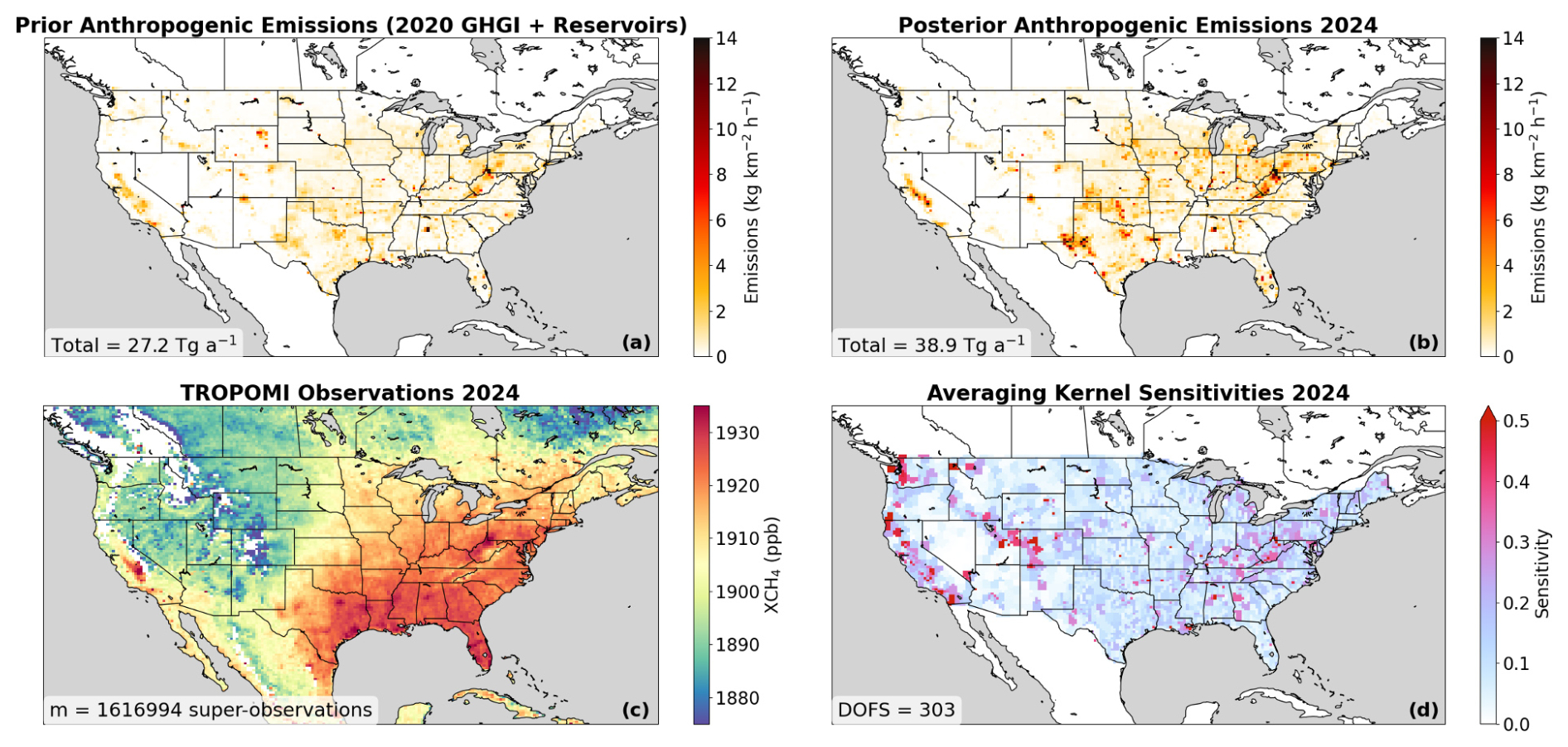
Figure 1 CONUS anthropogenic methane emissions, TROPOMI observations, and inversion averaging kernel sensitivities for 2024. Values are annual means. (a) Prior emissions from the EPA Greenhouse Gas Inventory (GHGI) with added contribution from hydroelectric reservoirs (Delwiche et al., 2022). Total emission is inset. (b) Posterior anthropogenic emissions from the mean of our inversion ensemble. (c) TROPOMI observations of dry column methane mixing ratios (XCH₄), averaged on the 0.25° × 0.3125° GEOS-Chem grid as hourly super-observations (see text). Low values reflect topography. White grid cells have no observations. Total number of super-observations is inset. (d) Averaging kernel sensitivities for the inversion (diagonal elements of the averaging kernel matrix) on the state vector grid. The sum of averaging kernel sensitivities, representing the degrees of freedom for signal (DOFS), is inset.

2.1 Observations and boundary conditions

We use the blended TROPOMI+GOSAT XCH₄ observation product (Balasus et al., 2023) which corrects the operational TROPOMI data of Lorente et al. (2021) with a machine-learning (ML) algorithm trained on collocated GOSAT data. GOSAT is more precise and less subject to surface and aerosol artifacts because it uses a CO₂ proxy retrieval method for the 1.6 µm absorption band (Parker et al., 2020), whereas TROPOMI uses a full-physics retrieval method for the 2.3 µm absorption band. But GOSAT data are ∼ 200 times sparser than TROPOMI, and the blended TROPOMI+GOSAT product thus combines the density of TROPOMI observations with the quality of GOSAT observations. We refer to this blended product as TROPOMI in the text.

TROPOMI observations are limited to land and cloud-free scenes, and are fairly distributed across seasons over the domain of Fig. 1 (Fig. S1 in the Supplement). The number of observations ingested each year varies from 7.6 to 10.4 million. We average observations over the 0.25° × 0.3125° GEOS-Chem grid for each orbit to create super-observations (Eskes et al., 2003), where the reduction in retrieval error from averaging accounts for error correlations as described by Chen et al. (2023).

Smoothed TROPOMI concentrations applied as boundary conditions along the edges of Fig. 1 are produced on a 2.0° × 2.5° grid following Estrada et al. (2025) by sampling XCH₄ and its vertical distributions from a GEOS-Chem simulation with prior emission estimates, and correcting it with 15 d averages of TROPOMI observations over 8° × 10° domains. When such averages are not available, as for oceans, we apply a zonal mean correction for that latitudinal band. Using smoothed TROPOMI concentrations in this manner as boundary conditions ensures consistency with the observations used in the inversion. We estimate a 5–15 ppb error standard deviation on boundary conditions based on comparison with TCCON ground-based XCH₄ observations (Maasakkers et al., 2019).

2.2 Analytical inversion with the IMI

We apply the IMI (version 2.1; https://carboninversion.com, last access: 4 December 2025) to infer emissions by minimizing the Bayesian cost function with normal error statistics (Brasseur and Jacob, 2017):

$$\begin{array}{}\text{(1)}& \begin{array}{rl}J\left(\mathit{x}\right)& ={\left(\mathit{x}-{\mathit{x}}_{\mathit{A}}\right)}^T{{\mathbf{S}}_{\mathbf{A}}}^{-\mathrm{1}}\left(\mathit{x}-{\mathit{x}}_{\mathit{A}}\right)\\ & +\mathit{\gamma }{\left(\mathit{y}-\mathbf{K}\mathit{x}\right)}^T{{\mathbf{S}}_{\mathbf{O}}}^{-\mathrm{1}}\left(\mathit{y}-\mathbf{K}\mathit{x}\right),\end{array}\end{array}$$

where x is the state vector of emissions and boundary conditions, x_A is the prior estimate, y is the vector of observations, K = $\partial \mathit{y}/\partial \mathit{x}$ is the Jacobian matrix relating emissions to concentrations in GEOS-Chem, S_A is the prior error covariance matrix, S_O is the observational error covariance matrix, and γ is a regularization parameter to prevent overfit to the observations. S_A and S_O are taken as diagonals for lack of better information, and γ < 1 is needed to correct for error correlation between super-observations that is not accounted for in S_O.

The optimal estimate, $\widehat{\mathit{x}}$, is derived analytically by solving $\mathrm{d}J/\mathrm{d}\mathit{x}$ = 0 (Rodgers, 2000; Brasseur and Jacob, 2017), yielding:

$$\begin{array}{}\text{(2)}& \widehat{\mathit{x}}={\mathit{x}}_{\mathit{A}}+{\left(\mathit{\gamma }{\mathbf{K}}^{\mathbf{T}}{{\mathbf{S}}_{\mathbf{O}}}^{-\mathrm{1}}\mathbf{K}+{{\mathbf{S}}_{\mathbf{A}}}^{-\mathrm{1}}\right)}^{-\mathrm{1}}\mathit{\gamma }{\mathbf{K}}^{\mathbf{T}}{{\mathbf{S}}_{\mathbf{O}}}^{-\mathrm{1}}\left(\mathit{y}-\mathbf{K}{\mathit{x}}_{\mathit{A}}\right).\end{array}$$

The analytical solution provides explicit error characterization through $\widehat{\mathbf{S}}$, the posterior error covariance matrix:

$$\begin{array}{}\text{(3)}& \widehat{\mathbf{S}}={\left(\mathit{\gamma }{\mathbf{K}}^{\mathbf{T}}{{\mathbf{S}}_{\mathbf{O}}}^{-\mathrm{1}}\mathbf{K}+{{\mathbf{S}}_{\mathbf{A}}}^{-\mathrm{1}}\right)}^{-\mathrm{1}}.\end{array}$$

The averaging kernel matrix A = $\partial \widehat{\mathit{x}}/\partial \mathit{x}$ = $\mathbf{I}-\widehat{\mathbf{S}}{{\mathbf{S}}_{\mathbf{A}}}^{-\mathrm{1}}$ describes the sensitivity of the inversion to the true state. The diagonal elements of A, a_ii, are called averaging kernel sensitivities and measure the ability of the observations to infer emissions on the native state vector grid independently of the prior estimate, ranging from 0 (no ability) to 1 (complete ability). Emissions can still be quantified from the observations when averaging kernel sensitivities are low by spatial aggregation. The sum of averaging kernel sensitivities (trace of A) defines the degrees of freedom for signal (DOFS), estimating the total independent number of pieces of information from the observations.

The posterior error covariance matrix $\widehat{\mathbf{S}}$ does not account for uncertainties in inversion hyperparameters (prior error standard deviation, observational error standard deviation, regularization parameter, error distribution, etc.) which dominate the overall error (Chen et al., 2022b). As a more conservative estimate of uncertainties on our posterior emission estimates, we generate an ensemble of estimates with varied inversion hyperparameters, considering both normal and lognormal probability density functions (pdfs) for the prior emission error estimates (Table 1). Lognormal error pdfs may better characterize the heavy tail of emissions, particularly for the oil/gas sector (Yuan et al., 2015; Cui et al., 2019), and have the advantage of enforcing positivity in the solution. Lognormal error pdfs are accommodated in Eq. (1) by solving for ln x instead of x, which makes the forward model non-linear and requires solving for $\ln \widehat{\mathit{x}}$ iteratively. We solve this problem with the Levenberg–Marquardt algorithm (Chen et al., 2022b). The optimization is then for the median of x rather than the mean, which requires median-mean conversions as described by Hancock et al. (2025). To account for errors in the boundary conditions, we optimize each cardinal domain edge as part of the inversion following Nesser et al. (2024). In practice, we find edge corrections to range in magnitude from 0.5 to −21 ppb for 2024 with the highest corrections on the western edge. From the combinations of inversion hyperparameters in each column of Table 1, we generate an ensemble of 36 normal and 6 lognormal estimates. These combinations were chosen from an original pool of 72 inversion members that used a range of values from previous TROPOMI inversions (Nesser et al., 2024; Varon et al., 2022; Chen et al., 2022b), such that the prior terms of the posterior cost function match the expected normalized chi-square value of 1 to within the range 0.5 to 1.5, indicating a successful fit while avoiding overfit (Lu et al., 2022). We report the mean from the ensemble members (equal weighting for normal and lognormal pdfs) as our best estimate and the range across ensemble members as our uncertainty. We calculate our 2019–2024 emission trends using Ordinary Least Squares (OLS) regression on the mean estimates for each individual year and report the corresponding standard error from the regression. We also calculate trends for individual ensemble members and find that the regression standard error is typically a more conservative estimate of the trend uncertainty (Fig. S2).

Table 1 Hyperparameters of the inversion ensemble.

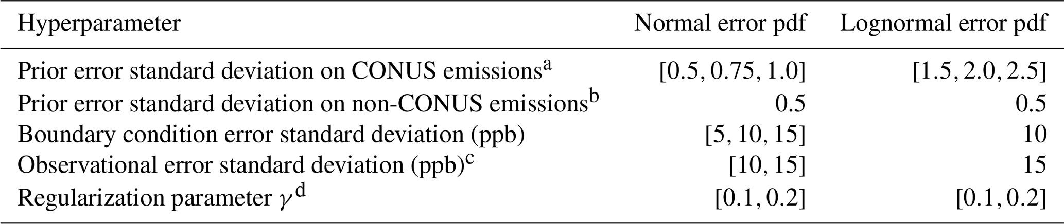
^a For state vector elements in CONUS; fractional error standard deviation for normal error pdf inversions, geometric standard deviation for lognormal error pdf inversions. ^b Fractional error standard deviation for state vector elements outside CONUS. The prior error for these elements follows a normal distribution in all cases. ^c Observational error used to construct S_O and including contributions from instrument, retrieval, and model transport errors. Nesser et al. (2024) found a mean observational error standard deviation of 11.5 ppb for TROPOMI over CONUS by applying the residual error method of Heald et al. (2004). The observational error is dominated by the retrieval error (Chen et al., 2023). ^d The regularization parameter γ ≤ 1 is designed to avoid overfit to the observations due to lack of implemented error correlation between individual observations and as diagnosed by the chi-squared test for the sum of prior estimate terms in the posterior cost function (Lu et al., 2021).

2.3 Forward Model

We apply the GEOS-Chem chemical transport model (version 14.4.1) as the forward model to relate emissions to atmospheric concentrations (Maasakkers et al., 2019) as expressed by the Jacobian matrix K in Eq. (1). The model is driven by NASA GMAO GEOS-FP meteorological fields at 0.25° × 0.3125 resolution (Lucchesi, 2017). We use the nested version of the model (Kim et al., 2015; Zhang et al., 2015) with a simulation domain of 19.25 to 54.75° N and 61.5625 to 130° W (domain of Fig. 1). Simulations are run for the full calendar year for each inversion year 2019–2024. The model includes methane sinks from atmospheric oxidation and soil uptake (Maasakkers et al., 2019). These are not directly optimized in the inversion but indirectly through the optimization of boundary conditions.

2.4 Prior estimates

Prior emission estimates for CONUS are summarized in Table 2. Anthropogenic emission estimates by sector are from the monthly GHGI at 0.1° × 0.1° grid resolution (Maasakkers et al., 2023) produced annually from 2012 to 2020. 2020 GHGI values are used as prior estimates for subsequent years in the inversion. GHGI does not include emissions from hydroelectric reservoirs, which we add from the Reservoir Methane Emissions inventory (ResME; Delwiche et al., 2022) and account for 7 % of anthropogenic emissions. Prior anthropogenic emission estimates for Mexico and Canada are from Scarpelli et al. (2020, 2022), who spatially allocate the UNFCCC reports on a 0.1° × 0.1° grid. Prior anthropogenic emission estimates for other countries in the model domain are IMI defaults (Estrada et al., 2025). For wetlands, we use the 2019 mean monthly estimates generated from the nine high-performance members of WetCHARTs v1.3.1 (Bloom et al., 2021) as prior estimate for all inversion years. Other minor natural sources include daily open fires from the Global Fire Emissions Database (GFED4) (Randerson et al., 2017), geological seeps (Hmiel et al., 2020), and termites (Fung et al., 1991).

Table 2 Methane emissions in the contiguous US (CONUS).

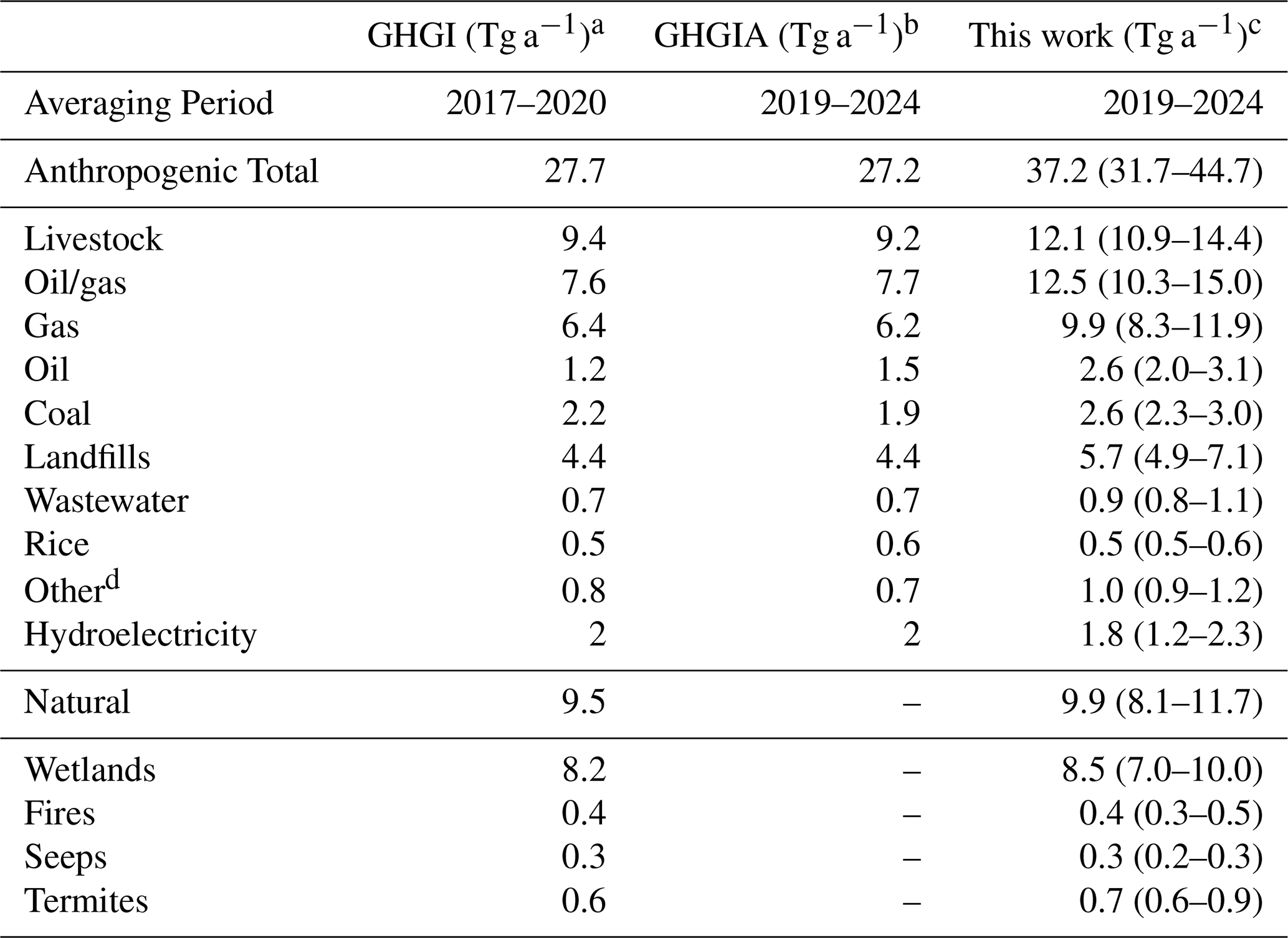
^a Mean of 2017–2020 U.S. EPA Greenhouse Gas Inventory (GHGI) for anthropogenic sources, with hydroelectric reservoir emissions added (Delwiche et al., 2022).
^b Mean of 2019–2024 Greenhouse Gas Inventory and Analysis for the United States (GHGIA) for anthropogenic sources, with hydroelectric reservoir emissions added (Delwiche et al., 2022).
^c Annual mean best posterior estimates over averaging period (2019–2024), with ranges from the inversion ensemble in parentheses.
^d Fossil fuel combustion, industrial processes, and agricultural burning.

Prior estimates for a given year do not include information from posterior results for the previous year, as would be done in a Kalman filter, in order to apply consistent corrections to the bottom-up estimates from year to year. The inversion optimizes annual posterior estimates only, assuming that the relative seasonality in the prior emissions is correct. That seasonality is mainly driven by wetlands. Seasonal variability in the GHGI is small and mainly driven by temperature-dependent emissions from livestock manure.

2.5 State vector clustering and sectoral attribution

We apply the IMI's smart clustering algorithm (Estrada et al., 2025) to generate a multi-resolution state vector that aggregates native grid cells in areas with weak emissions and low observation density, while maintaining native 0.25° × 0.3125° grid resolution in areas with strong emissions and high observation density. The same state vector clustering is used for all annual inversions and is based on the average observation density for 2019–2024 when applying the algorithm. We force clusters to respect state boundaries to avoid aggregation error on the calculation of state total emissions.

The number of state vector elements defining the resolution of the inversion should maximize the DOFS while remaining computationally affordable. We determined the optimal number before running the inversion by estimating the DOFS for varying state vector sizes in the IMI preview as described by Estrada et al. (2025). We choose a state vector dimension of 2600 as this is where the gain in the DOFS plateaus. Additionally, we impose a maximum cluster size of 10 grid cells per element to maintain relatively high resolution across the domain.

The inversion returns posterior annual emissions on the 0.25° × 0.3125° grid. Results are then aggregated nationally, by state, or by sector. Sectoral attribution is done by applying the posterior/prior emission ratio in each grid cell to correct the prior sectoral emissions in that grid cell. Spatially aggregated posterior emissions by sector are obtained by applying the summation matrix W with rows containing the relative contributions from individual sectors to emissions from each state vector element (Nesser et al., 2024). This reliance on the distribution of the prior emissions can lead to errors in sectoral attribution of the posterior/prior correction in regions where there is spatial overlap between sectors not resolved by the inversion. We characterize this error following Hancock et al. (2026) with the reduced averaging kernel matrix A_red:

$$\begin{array}{}\text{(4)}& {\mathbf{A}}_{\mathbf{red}}={\mathbf{WAW}}^{*},\end{array}$$

where W^* is the Moore–Penrose pseudoinverse matrix.

3 Results and discussion

3.1 Evaluation of inversion results

We evaluate our inversion results by comparing the GEOS-Chem simulation with posterior emissions (Fig. 1) to the TROPOMI observations used in the inversion and to independent observations from surface, aircraft, and tower observations in the NOAA CH₄ GLOBALVIEWplus v7.0 data product (Schuldt et al., 2024). Following Lu et al. (2022), NOAA observations are sampled during daytime hours (10:00–16:00 local time) and only include observations within 3 standard deviations from the daily mean, or 2 standard deviations if the standard deviation is greater than 30 ppb. We compare the model to the annual ensemble mean observations for each site for 2019–2023. Figure 2 shows improvements in RMSE and mean bias in the TROPOMI residuals relative to the prior estimate (panels a and b), a shift of the residual distribution toward zero (panel c), and a general whitening of noise across the domain, indicating improved agreement with the observations. Independent observations (panel d) show a 5.6 ppb improvement in mean bias relative to the prior estimate and a 5.3 ppb improvement in RMSE. The coefficient of determination (R²) increases from 0.61 to 0.74. Independent observation sites with the highest remaining bias tend to be close to high emitting regions (e.g. Permian basin, Appalachian basin), where local influences in surface air may be difficult to reproduce at the 25 km model resolution.

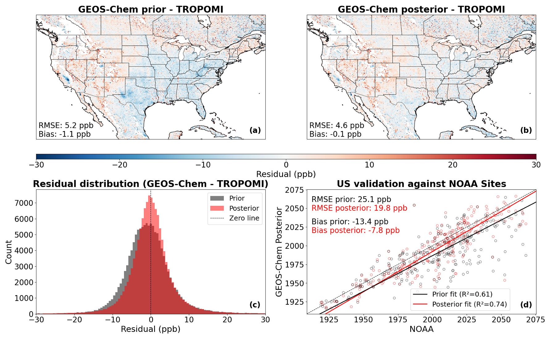
Figure 2 Evaluation of the prior and posterior emission estimates when implemented in the GEOS-Chem simulation. The top panels show the gridded annual mean residuals between GEOS-Chem and the TROPOMI observations for the (a) prior and (b) posterior simulations. Panel (c) shows the tightening of the residual distribution in the posterior estimate (red) versus the prior estimate (grey). Panel (d) shows comparison with independent NOAA site observations, where each point represents an annual afternoon mean. Root-mean-square errors (RMSE), mean biases, and reduced-major-axis regression lines are inset.

The averaging kernel sensitivities in Fig. 1 indicate regions where emissions are most informed by the observations versus the prior estimate (1 = fully, 0 = not at all). They are highest where prior emissions are high (because the prior error standard deviation is then high) and where the observation density is high. The values in Fig. 1 are for 2024 but observation density varies little between years and so do the averaging kernel sensitivities. Emissions for grid cells with low averaging kernel sensitivities cannot be quantified at 25 km resolution but can still be quantified as national, state, and sectoral levels as measured by the reduced averaging kernel matrix (Eq. 4). Statewide reduced averaging kernel sensitivities are listed in Table S1 in the Supplement. The national sectoral averaging kernel matrix is shown in Fig. S3 row by row to evaluate the ability of the inversion quantify emissions from individual sectors independently from the others on the national scale. Observations contribute substantial information for all sectors with averaging kernel sensitivities ranging from 0.3–0.7 (highest for oil/gas and coal) but still allowing for significant contribution from the prior estimate. Off-diagonal terms of the averaging kernel matrix indicate that the posterior for a given sector is influenced by the corrections to other sectors as would be the case for overlap. The mainly urban “other” emissions thus influence the posterior estimates for oil/gas (mainly from downstream distribution sources), livestock, and landfills. The remaining sectors are cleanly separated. Corrections to boundary conditions have averaging kernel sensitivities near unity and do not affect significantly the corrections to emissions.

3.2 National emissions and trends, 2019–2024

Table 2 summarizes sector-resolved methane emissions for CONUS. Our mean posterior estimate of total methane emissions is 47 Tg a⁻¹ with 10 Tg a⁻¹ from natural sources and 37 Tg a⁻¹ from anthropogenic sources for the 2019–2024 period. This estimate is 34 % higher than reported in the GHGI and 64 % higher for oil/gas emissions. Livestock and landfills are adjusted upward by 29 % and 30 %, respectively. Our results are consistent with other GOSAT and TROPOMI inverse studies, which find anthropogenic emissions in the range 30.0–42.7 Tg a⁻¹ (Turner et al., 2015; Maasakkers et al., 2021; Lu et al., 2022; Worden et al., 2022; Lu et al., 2023; Nesser et al., 2024). Results for individual sectors broadly agree with previous studies (Fig. S4) regardless of differences in time period, satellite product, prior inventory, and inversion methodology. There are discrepancies for coal and livestock with Turner et al. (2015), who used much sparser GOSAT observations, and for waste with Worden et al. (2022), who used much coarser resolution. Coal emissions have also decreased considerably since the 2009–2011 inversion years of Turner et al. (2015). Results for hydroelectric reservoirs show little departure from the ResME inventory used as prior estimate. Posterior emission estimates for wetlands and other natural sources also show little departure from the prior estimates.

Additionally, we compare our results in Table 2 to the Greenhouse Gas Inventory and Analysis (GHGIA; Desai et al., 2026), a recently released annual US inventory designed to be comparable with previous EPA GHGI inventories. This dataset does not include gridded information, but the national estimates and trends are broadly consistent with the GHGI. The underestimate identified in the GHGI still exists in the GHGIA. However, the GHGIA covers the period 1990–2024, allowing direct comparison of national trends with our posterior emission estimates.

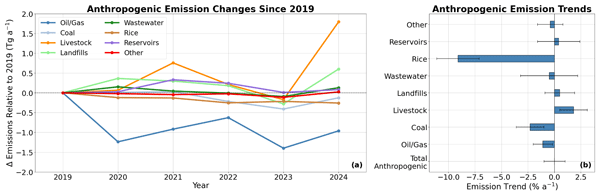
Figure 3 shows the change in posterior emission estimates for each year relative to 2019 and the sector-specific trends for 2019–2024. Trends are derived through Ordinary Least Squares (OLS) regression of the mean sectoral emissions for each year. Uncertainties are the corresponding standard error of estimates from the regression line. Total anthropogenic emissions are flat in our posterior estimate (0.0 ± 1.0 % a⁻¹) in conflict with the GHGIA trend (−1.8 ± 0.3 % a⁻¹), but consistent with global inversions of TROPOMI data (He et al., 2026; Pendergrass et al., 2025). However, this overall flat trend reflects offsetting trends from different sectors. Emissions from fuel exploitation declined over 2019–2024 by −1.1 ± 0.9 % a⁻¹ for oil/gas and −2.3 ± 1.3 % a⁻¹ for coal. The decrease of fossil fuel emissions supports the declining trends found in the GHGIA for oil/gas (−3.5 ± 0.6 % a⁻¹) and coal (−2.7 ± 1.2 % a⁻¹), which reflect lower emission intensities (Desai et al., 2026) and reduced production from underground mines (Penn et al., 2026). Livestock emissions including enteric fermentation and manure increase in our posterior estimate (1.8 ± 1.3 % a⁻¹), despite falling cattle populations (8 % since 2019; USDA NASS, 2025) that drive the GHGIA trend (−1.2 ± 0.2 % a⁻¹). However, the trend in our estimate is driven by a single year (2024). We do not find a significant trend in landfill emissions (0.5 ± 1.4 % a⁻¹), in contrast to a declining trend reported by the GHGI (and GHGIA) that Balasus et al. (2025) show to be an artifact from a switch in landfill emission models. For rice agriculture, we see a large decreasing trend (−9.1 ± 2.0 % a⁻¹), which may be due to increasing adoption of water-saving practices (Hardke et al., 2024) not accounted for in the GHGIA trend (1.6 ± 1.6 % a⁻¹).

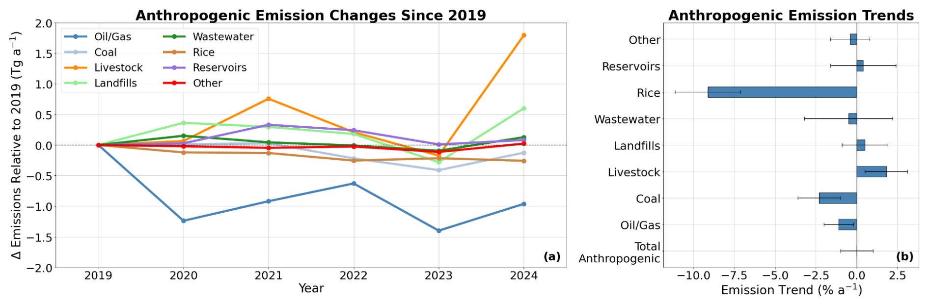
Figure 3 Changes in CONUS anthropogenic methane emissions relative to 2019 and trends by sector, 2019–2024. Values show the change in the annual mean posterior estimates relative to 2019. Trends are derived from ordinary least squares regression of emissions for individual years, and error bars are the standard error.

Methane intensity from the oil/gas sector is commonly defined as the total methane emissions along the oil/gas supply chain per unit of dry production of methane (Alvarez et al., 2018). We compute it using dry gas production data from the U.S. Energy Information Administration (EIA) assuming 85 % methane content (EPA, 1998). We find that the methane intensity decreased from 2.3 % to 1.9 % over the 2019–2024 period (Fig. 4). This continues the decreasing trend identified by Lu et al. (2023) for 2010–2019 and the consistent 2012–2020 trend in the GHGI. Our computed intensities are further consistent with the 2019 values computed using GOSAT and NOAA observations for 2019 (Lu et al., 2023) and for 2019 and 2023 values computed using TROPOMI (Shen et al., 2023; East et al., 2025). Lu et al. (2023) and Varon et al. (2023) found that declining intensities were due to increasing production with stable emissions, implying that emissions were decoupled from production. Here, we further find that actual emissions decrease while production increases, demonstrating recent improvements in emission management. Trends in emissions and intensities for individual oil/gas basins are discussed in Sect. 3.4.

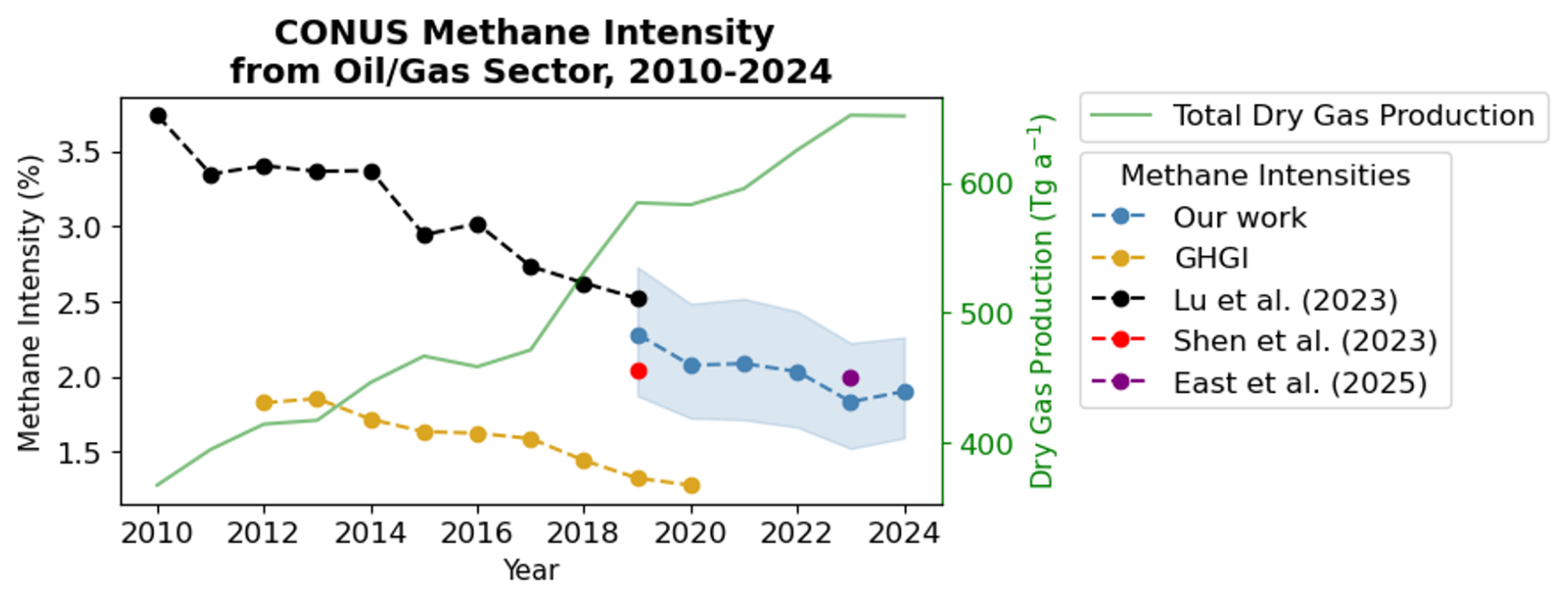
Figure 4 National methane intensity trends for the oil/gas sector in CONUS, 2010–2024. The 2019–2024 trend from this work (best posterior estimate and range from the ensemble) is compared to a 2023 TROPOMI inversion (East et al., 2025), a 2019 inversion of older TROPOMI retrievals (Shen et al., 2023), the 2010–2019 trend from an inversion of GOSAT and NOAA observations (Lu et al., 2023), and the GHGI trend extending to 2020. Total dry gas production of methane is from the U.S. Energy and Information Administration (U.S. EIA, 2025).

3.3 Emissions and trends for individual states

Figure 5 shows anthropogenic emission totals and trends for individual US states and Table 3 summarizes data for the top 10 emitting states, which together account for 55 % of total anthropogenic US emissions. Data for all states are in Table S1. Averaging kernel sensitivities for total emissions from individual states in Table S1 range from 0.07 (Rhode Island) to 0.72 (California), reflecting differences in both state sizes and magnitudes of emissions. Emissions from Rhode Island (the smallest US state) are weak and cannot be effectively separated from those in neighboring states. Averaging kernel sensitivities for the top 10 states in Table 3 are 0.46 for Illinois and 0.58–0.72 for other states, indicating a high level of state-specific observational information from the inversion.

Table 3 Emissions and trends for the top ten emitting US states^a.

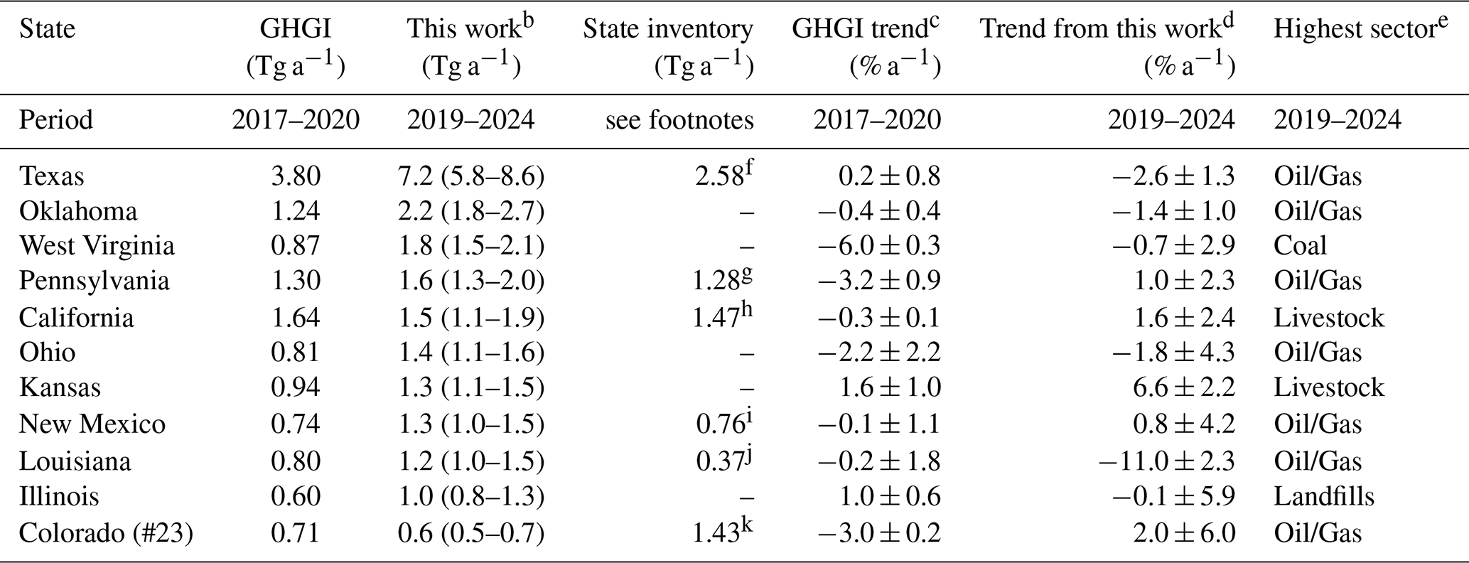
^a Mean emissions and linear regression trends ± standard error for the reported periods, for the top ten emitting states in our posterior estimate plus Colorado (discussed in the text). ^b Mean posterior estimate from our inversion, with uncertainty bounds in parentheses from the range of the inversion ensemble. State-level uncertainties are marginal posterior standard deviations and do not include covariance with neighboring states. ^c From a linear regression of GHGI estimates. ^d From a linear regression of the mean of the inversion ensemble for individual years. ^e As determined by the posterior emissions estimate. ^f 2022 (Allen et al., 2025). ^g 2019–2022 (Pennsylvania DEP, 2025). ^h 2019–2023 (California Air Resources Board (CARB), 2025). ⁱ 2021 (Bharadwaj et al., 2024). ^j 2018 (Dismukes, 2021). ^k 2017–2020 (Twyman et al., 2024).

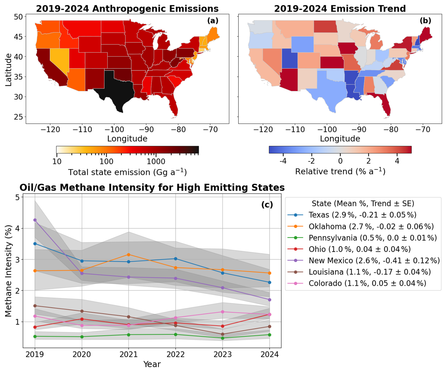
Figure 5 Mean 2019–2024 anthropogenic emissions, trends, and intensities for individual states. Panel (a) shows mean anthropogenic emissions on a log scale. Panel (b) shows the percent change per year from a linear regression of the emissions for each state. Panel (c) shows methane intensities from the oil/gas sector for the six states dominated by oil/gas emissions and Colorado. The trends and standard errors (SE) are from ordinary least squares regression of the mean intensity for each year. EIA data on individual state dry production for 2024 was unavailable at the time of writing, so we estimate dry production from marketed gas using the ratio of dry production to marketed gas in 2023.

Texas is the largest emitting state, responsible for 19 % of national anthropogenic emissions, primarily from oil/gas activity. Six of the top 10 states are dominated by oil/gas emissions, and all six show upward oil/gas adjustments relative to the GHGI: Texas (+121 %), Oklahoma (+100 %), Pennsylvania (+47 %), Ohio (+41 %), New Mexico (+98 %), and Louisiana (+69 %). Texas, Oklahoma, and New Mexico exhibit particularly high oil/gas sector methane intensities (Fig. 5). In general, we find that states with dominant fossil fuel emissions show declining trends and states with dominant livestock emissions show increasing trends. Texas, California, and Nebraska are the largest livestock emitters, reflecting their large animal populations, but national trends are disproportionately influenced by livestock emissions increases in Iowa (8.3 ± 4.8 % a⁻¹), Kansas (7.0 ± 2.1 % a⁻¹), and Missouri (5.4 ± 4.3 % a⁻¹). These increases cannot be explained by herd size, as livestock populations remained stable in Iowa, although with higher hog populations (USDA NASS, 2025), and declined in Kansas and Missouri. Dairy cattle numbers rose in Iowa and Kansas but insufficiently to account for the observed emission trend. Rice emissions are concentrated in Arkansas and Louisiana and drive the decline in Arkansas' methane emissions, possibly driven by changing agricultural practices (Hardke et al., 2024) with methane reduction benefits (Runkle et al., 2019; Karki et al., 2021), though attribution is complicated by declining summer precipitation during 2019–2024 (National Centers for Environmental Information (NCEI), 2025).

Twenty-one states within CONUS produce their own greenhouse gas inventories, independent of the GHGI, using either custom-built frameworks or the EPA State Inventory Tool (SIT) with state-specific inputs (EPA, 2025). Here, we examine the available state inventories for the top ten emitting states, plus Colorado in support of their strong regulatory efforts (Colorado General Assembly, 2019). We find that state-specific data do not always lead to improvements over the GHGI. Texas released its first state inventory in 2025 using a combination of national and state information (Allen et al., 2025). Its estimate is lower than both the GHGI (−32 %) and our estimate (−64 %), driven by an underestimate of oil/gas emissions. Louisiana's inventory (Dismukes, 2021), based on the EPA SIT tool, is considerably lower than both the GHGI and our estimate, largely due to differences in reported oil/gas and landfill emissions. Pennsylvania is one of the highest producers of natural gas and has long shown very low methane intensity in the oil/gas sector, as seen in Fig. 5 and in other studies (Cardoso-Saldaña and Allen, 2021; Lu et al., 2023). The state inventory for Pennsylvania (Pennsylvania DEP, 2025) uses the EPA SIT but applies Appalachian-specific emission factors and incorporates more information on well type and counts from private data. It reports oil/gas emissions 30 % higher than the GHGI, aligning with the range of uncertainty in our estimate. However, despite close agreement with our work for oil/gas, Pennsylvania inventory totals are slightly lower than the GHGI estimate due to very low reported landfill emissions, which are substantially lower than both the GHGI and our estimate. This discrepancy may arise from overestimated landfill gas recovery efficiencies used to calculate total emissions (Balasus et al., 2025; Wang et al., 2025).

California has adopted targets to reduce 75 % of landfill emissions by 2025 relative to 2014 and 40 % of manure management emissions by 2030 relative to 2013 (California Legislature, 2016), alongside comprehensive oil/gas regulations (California Air Resources Board (CARB), 2017). The California Air Resources Board (CARB) generates annual emission estimates using custom methodology and state specific activity data to track state emission goals. California is the only state among the top 10 where our inversion adjusted emissions downward from the GHGI (−7 %) with particularly large decreases for oil/gas (−20 %) and landfills (−30 %). Comparison with the CARB inventory (California Air Resources Board (CARB), 2025) shows closer agreement across all sectors except oil/gas, reflecting the accuracy of non-fossil California data sources and reporting programs (Appuhamy and Kebreab, 2018). Comparisons of our results for individual sectors with the California inventory are shown in Fig. S5.

New Mexico has mandated a < 2 % methane intensity for oil/gas operations by 2026, frequent leak detection and repair (LDAR), and restrictions on flaring and venting beginning in 2021 (New Mexico Oil Conservation Commission, 2021). The state is home to a subset of the Permian basin, where high methane intensities have previously been documented (Zhang et al., 2020; Schneising et al., 2020; Liu et al., 2021; Chen et al., 2022a; Shen et al., 2022; Varon et al., 2023). The state's inventory (Bharadwaj et al., 2024), based on detailed equipment-level data, yields higher emissions than the GHGI (+10 %) but remains below our estimate (26 % higher than GHGI). We find a substantial decline in methane intensity from 4.3 % in 2019 to 1.7 % in 2024, indicating that New Mexico has already achieved its target of < 2 %, though most reductions occurred before the 2021 regulations. This decline in intensity is consistent with studies over the New Mexico portion of the Permian basin. Varon et al. (2025) found a decrease from 4.5 % to 2.1 % during 2019–2023. Aerial surveys over the area show a similar downward trend, with Chen et al. (2022a) reporting intensities of 9.4 % in 2018–2020 and Donahue et al. (2026) reporting 2.1 % in 2024.

Colorado has targeted a 50 % reduction in greenhouse gas emissions by 2030 relative to 2005 (Colorado General Assembly, 2019), supported by oil/gas regulations including quarterly and semiannual LDAR, a ban on routine flaring, and a 2029 phaseout of pneumatic devices (Colorado Department of Public Health and Environment (CDPHE), 2025). Further emission controls on landfills were enacted in late 2024. We find downward adjustments for Colorado relative to the GHGI across all sectors except oil/gas, including livestock (−17 %), landfills (−23 %), and coal (−52 %). The oil/gas sector is 12 % higher than the GHGI estimate and corresponds to a mean oil/gas methane intensity of 1.1 %. We find an 18 % downward adjustment for anthropogenic emissions relative to the most recent Colorado Department of Public Health inventory (Colorado Department of Public Health and Environment (CDPHE), 2026), but both inventories are within the bounds of the inversion ensemble. The updated state inventory substantially improves agreement for oil/gas emissions, which were previously overestimated in earlier CDPHE inventories due to outdated leakage rates (Twyman et al., 2024; Nesser et al., 2024). With the new inventory, our estimate is within 10 % of the CDPHE oil/gas estimate.

3.4 Emissions and trends for oil/gas production fields

Figure 6 summarizes the oil/gas emissions and trends for the top 8 emitting oil/gas fields in CONUS. The annual mean reduced averaging kernel sensitivities for these fields are all 0.60 or above, except for Eagle Ford (0.44). Total methane emissions are dominated by the oil/gas sector, so that there is little error in attribution posterior/prior corrections to that sector. The Permian and Appalachian fields represent, respectively, 21 % and 14 % of CONUS oil/gas sector emissions with mean emissions of 2700 (2100–3400) Gg a⁻¹ and 1700 (1500–2300) Gg a⁻¹. Although the Appalachian's methane intensity is relatively low, its high production volume makes it one of the highest total emitters among US oil/gas fields. The Permian estimate is in the same range as other top-down estimates from Shen et al. (2022), Varon et al. (2023), Lu et al. (2023), and Omara et al. (2024). We find an average underestimate in the GHGI of 83 % across the top 8 oil/gas production fields with the largest adjustment in the Permian (+202 %) and the lowest adjustment to the Uinta Piceance (+28 %). We calculate methane intensities with the integrated emissions from the oil/gas supply chain, but upstream emissions from production are the dominant source in the top 8 oil/gas basins, so that methane intensity changes little if midstream or downstream emissions are excluded (Fig. S6). We find particularly high methane intensities in the Barnett (3.1 %), Permian (2.3 %), and San Juan (2.2 %). Oil-dominant fields, like the Permian, may exhibit high methane intensities due to insufficient gathering, processing, and midstream pipeline equipment for capturing associated gas from oil production (Lu et al., 2023; Omara et al., 2024; Varon et al., 2025). The Barnett and San Juan are gas-dominant fields that share common features: development peaked over a decade ago, production has since declined, and new investment has been limited. In contrast, gas-dominant fields with active development have some of the lowest intensities, including Haynesville (0.7 %), Appalachian (0.8 %), Anadarko (1.6 %), and Uinta-Piceance (1.7 %). The oil-dominant Eagle Ford, which also has low methane intensity (0.9 %), has rising gas production (and declining oil production) during the study period, suggesting increased investment in gas infrastructure.

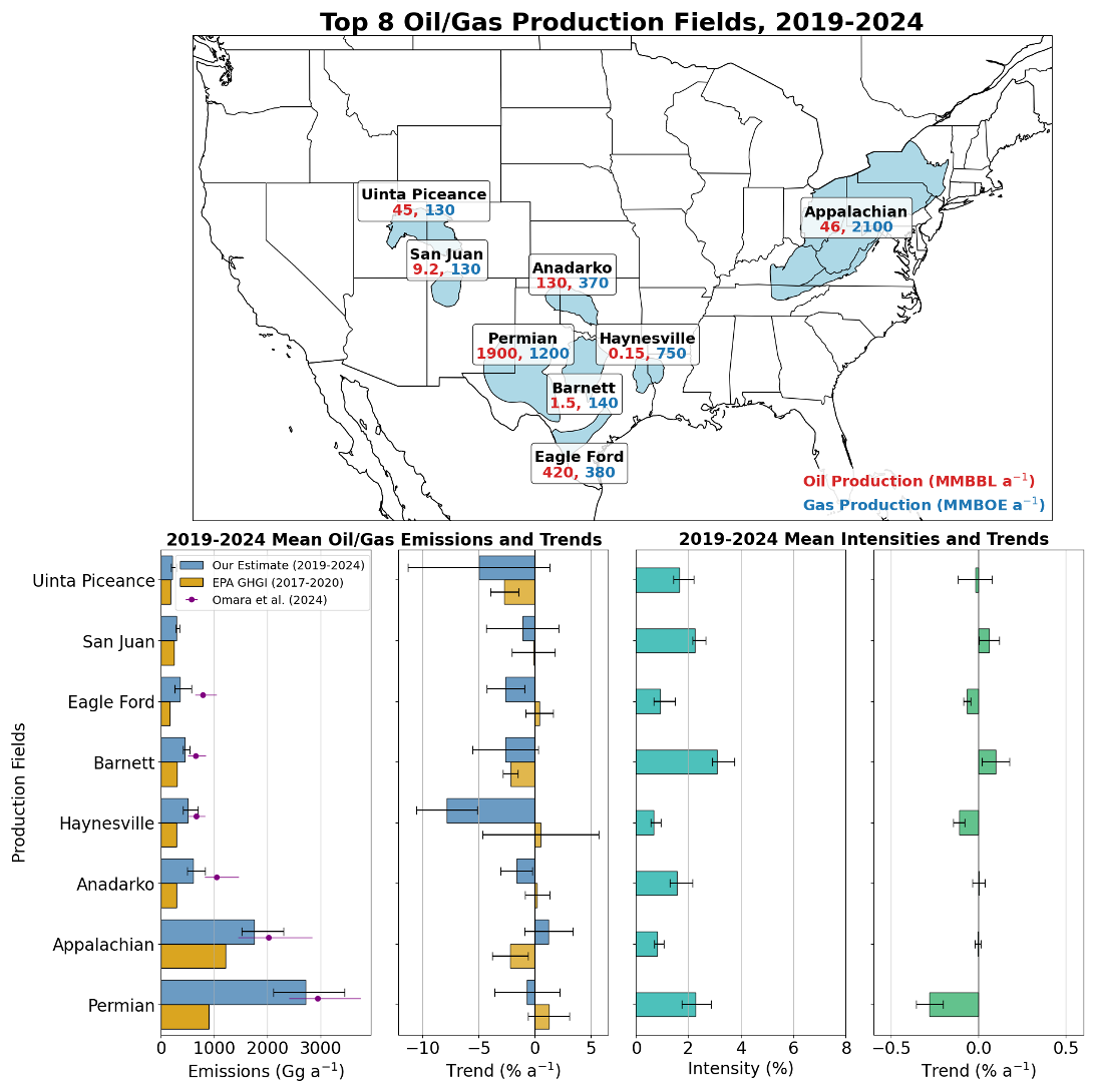
Figure 6 2019–2024 mean oil/gas production, emissions, emission intensities, and trends for the top eight oil/gas production fields in CONUS. Emissions and emission intensities are from the mean of our posterior estimates, with error bars representing the ranges from the inversion ensemble (for the 2019–2024 mean panels) or the standard error on the regression slopes (for the trends). Emission estimates from Omara et al. (2024) are for 2021 emissions. Trends are calculated using OLS regression on results for individual years. Production data were derived from the Enverus prism platform (Enverus, 2025). MMBBL is million barrels of oil and MMBOE is million barrels of oil equivalent. Oil/gas field boundaries are based on definitions in Omara et al. (2024).

All high-emitting production fields experience declining (Anadarko, Haynesville, and Eagle Ford) or flat emissions trends, consistent with findings for Texas oil/gas fields reported by Varon et al. (2025). The Haynesville and Eagle Ford fields increased production while reducing emissions, demonstrating improvements in emissions management. The San Juan and Barnett are the only fields in the top 8 with rising methane intensity. Their trends may reflect fixed emissions from aging infrastructure comprising a growing share of total emissions as gas production decreases.

4 Conclusions

We presented high-resolution annual methane emission estimates for the contiguous US (CONUS) from 2019 to 2024 using the open-source Integrated Methane Inversion (IMI 2.1) with TROPOMI satellite observations. The inversions used the EPA Greenhouse Gas Inventory (GHGI) as prior estimate. Our goal is to support the GHGI going forward with an inversion framework configured for consistent and transparent annual updates of US methane emissions. Annual results are visualized on a custom dashboard (https://laestrada.github.io/conus_emissions_viz/, last access: 4 January 2026.). Leveraging its open-source code, the system has been ported to the NASA Multi-Mission Algorithm and Analysis Platform as part of the U.S. Greenhouse Gas Center (U.S. GHG Center, 2025), demonstrating potential for annual updates and use by government and private stakeholders. It is also available on the Amazon Web Services (AWS) cloud.

We find that mean CONUS anthropogenic emissions for 2019–2024 are 37 Tg a⁻¹, 34 % above the GHGI, with oil/gas emissions 64 % above the GHGI. We find no significant 2019–2024 trend in CONUS emissions, but this result reflects an offset between decreasing trends from oil/gas (−1.1 ± 0.9 % a⁻¹), coal (−2.3 ± 1.3 % a⁻¹), and rice (−9.1 ± 2.0 % a⁻¹) emissions, and increasing trends from livestock (+1.8 ± 1.3 % a⁻¹) emissions. The signs of sectoral trends broadly agree with the latest GHGI trends reported for 2017–2020 (except rice). National oil/gas methane intensity declined from 2.3 % to 1.9 % over the 2019–2024 period, continuing a previously reported declining trend for 2010–2019 and consistent with the GHGI. Unlike the 2010–2019 trend, however, we find that emissions themselves have declined, demonstrating improved management to reduce emissions.

We find that over half of US anthropogenic methane is emitted from just ten states. Texas alone contributes 19 %. Texas and other oil/gas-dominated states (Oklahoma, New Mexico, Ohio, Louisiana) show declining or flat trends over 2019–2024. New Mexico's oil/gas intensity fell from 4.3 % in 2019 to 1.7 % in 2024, effectively meeting the state's < 2 % target for methane intensity from the oil/gas sector. Kansas and Iowa show significant 2019–2024 increases in emissions driven by livestock. Arkansas shows decreasing emissions driven by rice agriculture. Emission inventories constructed by individual states using state-specific data do not always improve upon GHGI estimates.

Most major US oil/gas production fields show stable or declining emissions. The Haynesville and Eagle Ford show rising production with falling emissions, indicating improved gas capture rates. Rising methane intensities are found in just two fields and are driven by declining production, suggesting a dominance of aging or abandoned infrastructure. Gas-dominant fields generally exhibit lower intensities than oil-dominant fields, though the low-intensity Appalachian basin now ranks as a top-emitting field due to its high level of gas production.

This work highlights how sustained satellite-based inversions can identify trends and discrepancies in methane emissions across regions and sectors, and play an increasingly important role in monitoring US methane emissions going forward. Integrating this top-down information into the GHGI to improve the bottom-up representation of processes would provide a powerful platform for emission reporting and for supporting action to reduce emissions.