Surface PM_2.5 air pollution in 2022 India: emission updates, WRF-Chem model evaluation, and source attribution

India experiences some of the highest fine particulate matter (PM_2.5) concentrations globally. Understanding the spatiotemporal variations of PM_2.5 and its source attribution requires robust air quality modeling supported by up-to-date emission inventories. Here we present the first WRF-Chem model evaluation and source attribution analysis for India for 2022, supported by updates in sectoral emission inventories and model parameterizations. We have incorporated an updated residential emission inventory reflecting recent transitions to cleaner fuels in Indian households and develop a plant-level inventory for Indian coal-fired power plants. Further major improvements include model updates to the secondary organic aerosol scheme and an improved representation of near-surface pollutant mixing. Collectively our improvements result in a simulation with annual PM_2.5 bias of only 0.2±16.9 µg m⁻³ (0±31 %) across 288 surface monitoring sites in South Asia. We simulate an annual population-weighted (PW) mean PM_2.5 concentration of 47.4 µg m⁻³. Compared to earlier studies, in 2022 India's residential sector remained the dominant source of PM_2.5 in the Indo-Gangetic Plain, but ranked second nationally in PW mean PM_2.5 concentrations (15 %, 7.3 µg m⁻³). Industrial emissions emerged as the largest domestic contributor to national PW mean PM_2.5 (18 %, 8.6 µg m⁻³), with urban hotspots including Delhi and Mumbai. Power sector contributions ranked third nationally (13 %, 6.1 µg m⁻³) and were particularly influential in central India. Transboundary transport contributed more than any individual domestic source nationally (27 %, 12.8 µg m⁻³) with largest impacts in western India. These findings highlight the benefits of India's partial residential sector transition toward cleaner fuels, while underscoring the future benefits of controlling industrial and power sector air pollutant emissions.

1 Introduction

Long-term exposure to elevated ambient fine particulate matter (PM_2.5) is a major risk factor for human health and premature mortality globally (Institute for Health Metrics and Evaluation, 2024). India has among the highest surface PM_2.5 concentrations worldwide, leading to an estimated 1.0 to 2.1 million premature deaths annually (Lelieveld et al., 2015; Health Effects Institute, 2024). To address the severe air pollution challenges, the Indian government has proposed and implemented measures aimed at reducing emissions of PM_2.5 and its precursors, including the National Clean Air Program (NCAP) launched in January 2019 (Ganguly et al., 2020). Despite an observed reduction in surface PM_2.5 levels across India during 2018 to 2022, aided by favorable meteorology, annual PM_2.5 pollution in ∼80 % of non-attainment cities with continuous monitors still exceeded the country's annual standard of 40 µg m⁻³ in 2022 (Xie et al., 2024). In addition, future PM_2.5 pollution in north India is projected to worsen under global warming (Zhou et al., 2024), highlighting the need for strengthened mitigation measures. Effective regulation design and implementation depend on understanding spatiotemporal distributions of PM_2.5 across India and the contribution of various emission sources. Given the complex interactions of atmospheric physical and chemical processes across India, robust emissions and air quality modeling are essential to address these questions.

Previous modeling studies have quantified the source contributions to India's annual ambient PM_2.5 pollution levels during 2015 to 2019 (Conibear et al., 2018; Guo et al., 2018; Reddington et al., 2019; Singh et al., 2021; Pai et al., 2022; Chatterjee et al., 2023; Kumar et al., 2025; Venkataraman et al., 2018). Across these studies, the residential sector consistently emerged as the leading contributor to PM_2.5 exposure nationwide, accounting for 21 % to 52 % of the national annual population-weighted (PW) mean PM_2.5 concentrations, with the range reflecting whether transboundary transport of residential emissions from adjacent countries were attributed to the residential sector. This dominance stems from inefficient and incomplete small-scale combustion of solid fuels in households, which produces substantial primary PM_2.5 emissions. In the literature, the power and industrial sectors were often among the largest national PM_2.5 sources after the residential sector, but their relative importance varied across studies, depending on the anthropogenic emission inventory applied. The power sector has been the dominant source of sulfur dioxide (SO₂, a key precursor of secondary inorganic PM_2.5) emissions since 2015 (Venkataraman et al., 2018), primarily due to India's fast-growing electricity demand and heavy dependence on coal, with only about 3 % of coal-based power plants equipped with flue gas desulfurization (FGD) systems in 2022 (National Environmental Engineering Research Institute, 2024). The industry sector was a major source of primary PM_2.5 and SO₂ emissions in 2015, and its emissions were projected to continuously increase from 2015 to 2050 (Venkataraman et al., 2018). In addition to these anthropogenic sources within India, studies identified a 20 %–28 % contribution from background (transboundary plus natural) sources to national mean PM_2.5 in India in 2016 (Singh et al., 2021; Pai et al., 2022).

Amid India's fast development, surging energy demand, and ongoing air quality regulations, more recent source contributions to PM_2.5 concentrations across the country remains unclear. Specifically, the promotion of cleaner fuels in the residential sector and the continued growth of coal-based electricity generation in the power sector have not been incorporated into existing PM_2.5 attribution studies. In addition, previous PM_2.5 modeling studies for India primarily focused on years before the NCAP baseline year of 2017, when relatively few surface PM_2.5 measurement sites existed and thorough model evaluation was thus not possible (Schnell et al., 2018; Guo et al., 2018; Singh et al., 2021; Pai et al., 2022; Agarwal et al., 2024). Given the need for up-to-date source attribution studies to guide India's future air quality interventions (e.g., the next phase of the NCAP), more rigorous modeling studies with updated emissions and robust model evaluation that disentangle the source contributions to India's surface PM_2.5 pollution in recent years are needed.

Here we present the first air quality modeling analysis for India using updated emissions for 2022, supported by key improvements in sectoral emission inventories and model parameterizations. We incorporate revised residential emissions that capture household transitions from solid fuels to liquefied petroleum gas (LPG), develop a refined plant-level inventory for coal-fired power generation, and update model treatments of secondary organic aerosol (SOA) formation and pollutant near-surface mixing. Using this enhanced inventory and model schemes, we conduct a rigorous evaluation of simulated PM_2.5 concentrations against observations from 288 surface monitoring sites and satellite-derived aerosol optical depth (AOD) retrievals across India and adjacent regions. We then quantify the contributions of nine emission sources to surface PM_2.5 pollution across India in 2022: eight domestic sources (six anthropogenic and two natural) and a transboundary source (all sources combined as one), providing critical insights for targeted air quality policy interventions.

2 Methods

2.1 WRF-Chem model

We use a recent version of the Weather Research and Forecasting model coupled with Chemistry (WRF-Chem, version 4.6.1) primarily developed by the National Center for Atmospheric Research (NCAR) (Grell et al., 2005). WRF-Chem is a mesoscale air quality model that online couples atmospheric chemistry (including aerosols) and meteorology (Fast et al., 2006; Chapman et al., 2009), allowing the simulation of the aerosol feedback on regional meteorology that are particularly critical in regions with high aerosol loadings (Zhou et al., 2019; Sharma et al., 2023; Huang et al., 2023). WRF-Chem is thus widely used to simulate surface PM_2.5 pollution over India (Govardhan et al., 2019; Agarwal et al., 2024; Venkataraman et al., 2024; Xie et al., 2024).

2.1.1 Model Configuration

We conduct simulations for 2022, the most recent year with available emission inventories for India (Sect. 2.2), using one month to represent each season: January for winter, April for pre-monsoon, July for monsoon, and October for post-monsoon (Sect. S1.1 in the Supplement). This four-season structure is widely adopted in recent literature to represent the distinct pollution and meteorological characteristics of each season (Lan et al., 2022; Venkataraman et al., 2024; Zhou et al., 2024; Xie et al., 2024; Kumar et al., 2025). We use a single domain covering India and adjacent regions (57–103° E, 4–39° N) with a horizontal resolution of 27 km (Fig. 1). There are 37 vertical layers extending from the surface to 50 hPa, with 10 to 15 layers below 1000 m above ground level, depending on local terrain heights. For meteorological initial and lateral boundary conditions, we use the hourly ERA5 climate reanalysis dataset at 0.25° × 0.25° resolution. To prevent drifting effects in simulated meteorological fields, we reinitialize WRF-Chem meteorology with ERA5 every 48 h, following our previous studies (Zhou et al., 2022; Xie et al., 2024). The chemical initial and boundary conditions are provided by the 6-h output from the Whole Atmosphere Community Climate Model (WACCM) (Gettelman et al., 2019; Emmons et al., 2020).

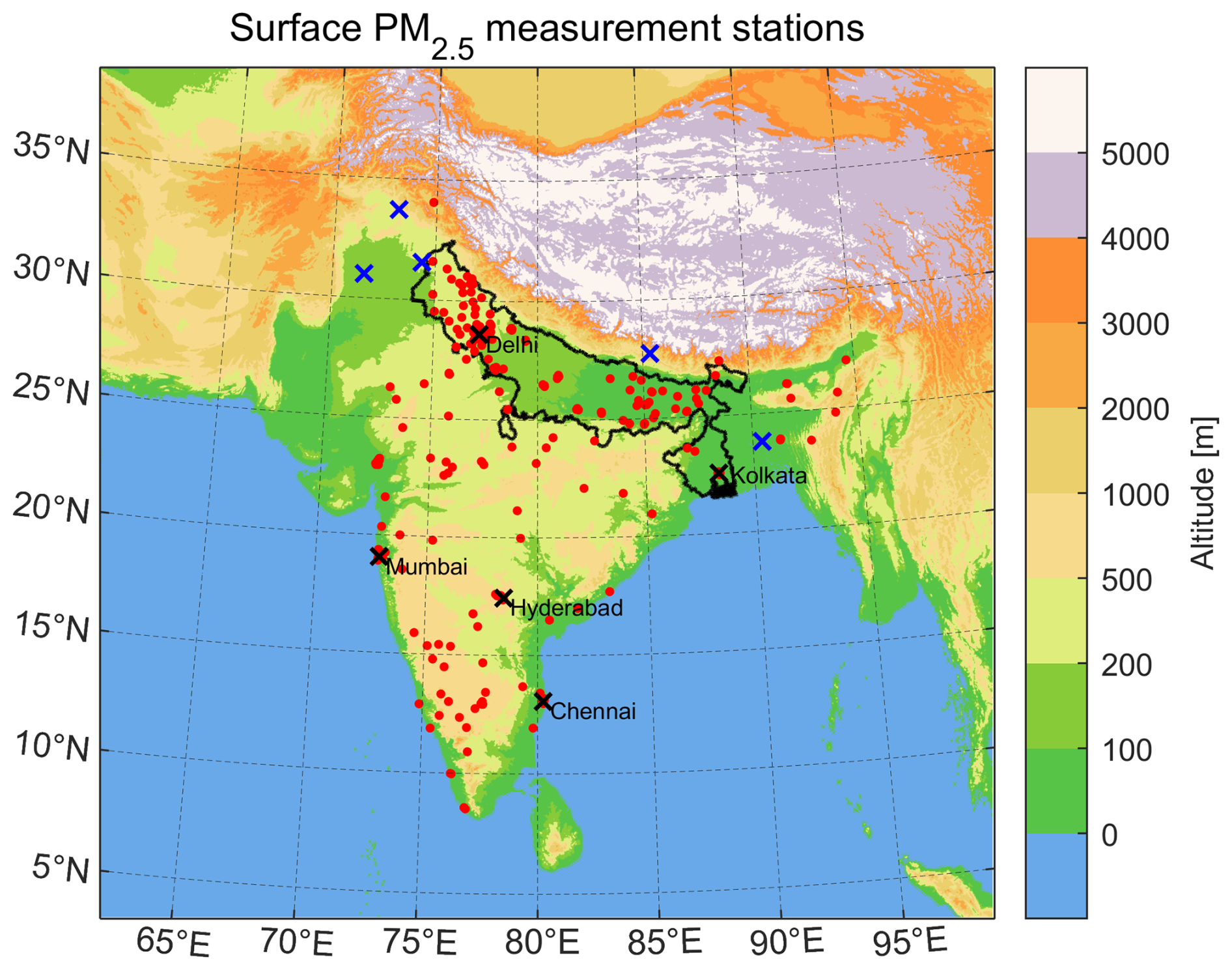
Figure 1 WRF-Chem modeling domain and surface PM_2.5 measurement stations utilized in this study. The base map shows the WRF-Chem modeling domain, with colors representing the terrain height in the model. The 288 surface PM_2.5 measurement sites used in this study are marked as follows: Red dots represent the continuous monitoring stations from the Indian Central Pollution Control Board (CPCB) network; the black and blue crosses represent the stations from U.S. Air Now network in India and adjacent countries, respectively. Thick black lines represent the boundary of the Indo-Gangetic Plain (IGP), which includes Delhi, Punjab, Haryana, Uttar Pradesh, Bihar, and West Bengal. We also label the five major cities of Delhi, Mumbai, Kolkata, Hyderabad, and Chennai, where U.S. Air Now PM_2.5 measurements were available in India.

We configure WRF-Chem with the following chemical schemes: the Carbon Bond Mechanism Z (CBMZ) gas-phase chemistry scheme (Zaveri and Peters, 1999), and the 4-bin version of the MOdel for Simulating Aerosol Interactions and Chemistry (MOSAIC) aerosol scheme with aqueous chemistry (Zaveri et al., 2008). The selected MOSAIC scheme simulates major aerosol species, including primary organic aerosols (POA), black carbon (BC), sulfate (${\mathrm{SO}}_{\mathrm{4}}^{\mathrm{2}-}$), nitrate (${\mathrm{NO}}_{\mathrm{3}}^{-}$), ammonium (${\mathrm{NH}}_{\mathrm{4}}^{+}$), sodium (Na⁺), chloride (Cl⁻), and other inorganic aerosols (OIN, including both natural dust and anthropogenic combustion and non-combustion dust). Each aerosol species is distributed across four size bins, with the first three bins (diameters ≤2.5 µm) contributing to PM_2.5 dry mass. Aerosols are assumed to be internally mixed inside each bin for optical property calculations. Under this configuration, the water uptake and hygroscopic growth properties of aerosols are calculated based on the bulk composition of the internally mixed particles (Zaveri et al., 2008). Major configurations for physical schemes are provided in Sect. S1.2 in the Supplement.

Natural emissions of dust and biogenic non-methane volatile organic compounds (NMVOCs) are calculated online within WRF-Chem. For dust emissions, we use the Goddard Chemistry Aerosol Radiation and Transport (GOCART) dust module (Ginoux et al., 2001). The GOCART dust emission scheme is widely used in aerosol modeling due to its relatively simple input requirements. Specifically, the GOCART scheme calculates dust emission fluxes using surface erodibility, 10-m wind speed, threshold soil moisture, and threshold wind speed, distributing dust aerosols into five size bins that partially overlap with the MOSAIC aerosol scheme's PM_2.5 bins. For biogenic NMVOCs, we use the Model of Emissions of Gases and Aerosols from Nature (MEGAN, version 2.06) (Guenther et al., 2006). MEGAN uses leaf area index (LAI), plant functional types (PFTs), and WRF-Chem-simulated meteorology to calculate emissions for 134 chemical species, which are subsequently mapped into the CBMZ gas-phase mechanism. Anthropogenic emissions, including emissions of open burning are described in Sect. 2.2.

Based on the model configuration, PM_2.5 dry mass in WRF-Chem is calculated using Eq. (1):

$$\begin{array}{}\text{(1)}& \begin{array}{rl}{\mathrm{PM}}_{\mathrm{2.5}}& ={\sum }_{i=\mathrm{1}}^{i=\mathrm{3}}\left({\mathrm{POA}}_i+{\mathrm{BC}}_i+{\mathrm{OIN}}_i+{\mathrm{SO}}_{{\mathrm{4}}_i}^{\mathrm{2}-}\right.\\ & \left.+{\mathrm{NO}}_{{\mathrm{3}}_i}^{-}+{\mathrm{NH}}_{{\mathrm{4}}_i}^{+}+{\mathrm{Na}}_i+{\mathrm{Cl}}_i\right)\end{array}\end{array}$$

Here, i indicates the aerosol bin used in WRF-Chem.

2.1.2 Model Updates

We implement the simple SOA scheme from the GEOS-Chem global chemistry transport model into WRF-Chem 4.6.1, as the selected WRF-Chem chemical option treats POA as non-volatile and does not include SOA. The simple SOA scheme uses a fixed-yield approach to estimate SOA and SOA precursor (SOAP) emissions from biogenic and combustion sources. For biogenic sources, SOA (SOAP) mass yields are assumed to be 1.5 % (1.5 %) from isoprene and 5 % (5 %) from both monoterpenes and sesquiterpenes. For combustion sources, no SOA is directly emitted. However, SOAP mass yields are assumed to be 1.3 % (6.9 %) from biomass (fossil fuel) combustion carbon monoxide (CO). SOAP is converted to SOA with a fixed lifetime of 24 h (Pai et al., 2020; Miao et al., 2020). Designed as a computationally efficient alternative, the simple SOA scheme approximates SOA concentrations without mechanistically modeling the formation and fate of individual aerosol species or explicit thermodynamic partitioning (Pai et al., 2020). The simple SOA scheme has demonstrated performance comparable to more complex, process-based SOA schemes (Pai et al., 2020; Miao et al., 2021). For simplicity, the predicted SOA mass from the simple SOA scheme is added to the POA variable to represent total organic aerosols in the model, as shown in Eq. (1). A discussion on the application of the simple SOA scheme in our simulation is provided in Sect. S1.3 in the Supplement.

We improve near-surface mixing of chemical species by setting a minimum exchange coefficient for air pollutants in the selected boundary layer scheme, following a previous study that found WRF-Chem's weak nighttime mixing led to overestimated diurnal variations of PM_2.5 (Du et al., 2020).

2.2 Anthropogenic emissions

2.2.1 Adoption of existing 2022 emission inventories

We use recent release of two global emission inventories for our 2022 WRF-Chem simulation: the Community Emissions Data System (CEDS, version 2024-07-08) and the Emissions Database for Global Atmospheric Research (EDGAR, version 8.1). Both inventories provide gridded emissions for years until 2022 and are widely used for air quality research. We adopt monthly gaseous emissions of SO₂, nitrogen oxides (NO_x), ammonia (NH₃), carbon monoxide (CO), and NMVOCs in 2022 from CEDS at 0.5° × 0.5° resolution (Hoesly et al., 2018). In addition, we obtain monthly particulate matter emissions of primary organic carbon (POC), BC, primary PM_2.5, and PM₁₀ emissions in 2022 from EDGAR at 0.1° × 0.1° resolution (Crippa et al., 2018), as CEDS does not provide primary PM_2.5 and PM₁₀ emissions. We spatially interpolate CEDS and EDGAR inventories to the 27-km resolution WRF-Chem grid using a mass-conservative method. We use the satellite-derived daily Fire INventory from NCAR (FINN, version 2.5.1) to represent open burning emissions of agricultural and municipal waste, as well as smoke emissions from wildfires (Wiedinmyer et al., 2023). To avoid double counting, we exclude open burning emissions from the global inventories described above when they already include this source.

To better capture India's recent increasing displacement of solid fuels by LPG for clean residential energy use (Ganguly et al., 2020), we adopt a 2022 emission inventory developed at the Indian Institute of Technology Delhi. This new residential inventory applies regression analysis to evaluate residential fuel usage, considering recent changes in consumption patterns and updated data on cleaner fuels (Velamuri et al., 2024). Thus, reductions in emissions from the residential sector are better represented than in the flat residential emission trends provided in EDGAR and CEDS from 2015–2022 (Fig. 2). Specifically, we adjust India's residential PM_2.5, SO₂, and NO_x emissions to align with state-level totals from this new residential inventory. In addition, we scale residential emissions of OC, BC, and CO in each Indian state using the factor calculated as the ratio of residential PM_2.5 emissions from the new inventory to those from EDGAR. We retain the original spatial patterns for all these scaled species. We provide a detailed comparison between residential emissions from the current global inventories and our updated inventory in Sect. 3.1.

Then, we replace the PM_2.5, SO₂, and NO_x emissions from coal-fired power plants in the updated inventory with a new national emission inventory for coal-fired power plants in India for 2022, which is detailed in Sect. 2.2.2.

In addition to these major updates to the emissions from India's residential and power sectors, we scale India's transportation-related PM_2.5 and coarse PM (PM_coarse, defined as particles with diameters >2.5 and ≤10 µm) emissions to match the state-level totals from a 2022 road dust emission inventory (Katiyar et al., 2024). This adjustment is motivated by our finding that transportation PM_2.5 emissions in EDGAR (i.e., 0.11 Tg across India in 2022) are underestimated compared with this locally-developed inventory in India (i.e., 0.33 Tg). Similarly, transportation PM_coarse emissions in EDGAR were only 0.01 Tg across India in 2022, significantly lower than the 1.04 Tg estimated by the recent Indian inventory. The discrepancy likely reflects EDGAR's omission of fugitive road dust PM emissions.

We provide details on aerosol mapping from EDGAR to WRF-Chem and on vertical allocation of emissions in Sect. S1.4–S1.5 in the Supplement.

2.2.2 Development of new 2022 coal-fired power plant emission inventory for India

We construct a new national emission inventory for coal-fired power plants in India in 2022, focusing on major air pollutants of SO₂, NO_x, and PM_2.5. The development of this inventory involves three major steps: (1) compiling and cross-checking unit-level information from multiple databases; (2) estimating plant-level emission factors based on a fuel linkage database linking coal used at specific plants to coal source regions, coal composition information, and a document estimating emissions factors from coal composition (U.S. Environmental Protection Agency, 1998); and (3) utilizing plant-level electricity generation and coal consumption data from the Central Electricity Authority (CEA) of India. Each of these steps is detailed in the following paragraphs.

We collect unit-level information from the Global Energy Monitor's (GEM)'s coal power plant database for July 2022. To align with India's central government data, as reflected in the Vasudha Foundation's datasets, we include all operating units from the GEM database. For captive units, we only include those documented by Vasudha. This results in a total of 210.6 GW in generation capacity, which matches the coal and lignite capacity reported by the CEA in July 2022. We retrieve the unit location from the GEM database. For units listed with “approximate” location coordinates in the GEM database, we update their coordinates using Google Earth.

We collect coal (including both coal and lignite, and hereafter) composition data for twelve domestic states and three international regions (Australia, South Africa, and Indonesia) through a literature review. We then convert the sulfur and ash content of coal into uncontrolled emission factors for SO₂ and PM_2.5 under various firing configurations for both bituminous and subbituminous coal based on a report (U.S. Environmental Protection Agency, 1998). In addition, the report provides NO_x emission factors that are independent of nitrogen content in the coal. Based on this information, we establish region-specific uncontrolled emission factors for both domestic coal and imported coal used in India's power plants (Table S1). We average the calculated emission factor for a given region if multiple coal composition datasets are found, and present one standard deviation from these calculated values as the uncertainty bounds. We assume no variation in coal composition within a given coal source region. Finally, we estimate plant-level emission factors for air pollutants, using Eq. (2).

$$\begin{array}{}\text{(2)}& {\mathrm{EF}}_{i,s}={\sum }_{r=\mathrm{1}}^n{\mathrm{EF}}_{r,s}\cdot F_{i,r}\end{array}$$

Where EF_i,s is the emission factor (g pollutant per kg coal) for power plant i and species s; EF_r,s is the emission factor of coal for source region r and species s; F_i,r is the fraction of coal supplied at plant i that is sourced from region r.

We retrieve daily plant-level coal consumption reports from the CEA for the calendar year 2022 and aggregate data by month. In addition, we retrieve monthly plant-level electricity generation reports from the CEA for the same year. While generation data is available for all plants throughout the year, the coal consumption data is missing for some plants. For plants with missing monthly coal consumption data, we estimate the missing values by applying the plant's generation-to-coal consumption ratio, averaged from months where both generation and coal consumption data are available. For plants with no coal consumption data for the entire year, we estimate the coal consumption using the reported generation, coal heating value, and heating rate using Eq. (3):

$$\begin{array}{}\text{(3)}& C_{i,j}=G_{i,j}\cdot {\mathrm{HR}}_i/{\mathrm{TV}}_i\end{array}$$

Where C_i,j is the monthly coal consumption (tons) for power plant i and month j; G_i,j is the monthly electricity generation (MWh) for power plant i and month j; HR_i is the heating rate (MJ kWh⁻¹) for plant i, which represents the plant thermal efficiency; TV_i is the thermal value (MJ per kg coal) of coal used in plant i.

Finally, we estimate the monthly total emissions for air pollutants for each plant, using Eq. (4).

$$\begin{array}{}\text{(4)}& E_{i,j,s}=C_{i,j}\cdot {\mathrm{EF}}_{i,s}\cdot \left(\mathrm{1}-{\mathit{\eta }}_s\right)\end{array}$$

Where $E_i{,}_{i,s,}$ is the monthly total emissions (kg) for power plant i, month j, and species s; C_i,j is the monthly coal consumption (tons) for power plant i and month j; E_i,s is the emission factor (kg pollutant per t coal) of coal for plant i and species s; η_s is the removal efficiency for air pollutant species s, and we assume a 90 % removal rate (η=0.9) for PM_2.5 and no end-of-pipe controls for SO₂ and NO_x (η=0) following previous studies (Sengupta et al., 2022; Singh et al., 2024).

We do not account for NO_x emission from gas plant operation in 2022. According to the Indian Petroleum and Natural Gas Statistics 2022–2023, gas consumption for this fiscal year was ∼8 billion m³. Using the gas plant NO_x emission factors from the U.S. Environmental Protection Agency (USEPA) report, we estimate the total NO_x emissions from gas plant to range from 0.01 to 0.04 Tg yr⁻¹, which is far lower than those from coal-fired power plants (i.e., 4.56 Tg yr⁻¹).

Table 1 Emission scenarios for WRF-Chem simulations conducted in this study.

^a This includes emissions from six source sectors within India: power, industry, residential, transportation, agriculture (excluding open burning), and open burning.
^b We modify WRF-Chem to enable grid-level customization to turn dust and biogenic emission modules on and off.
^c This includes both anthropogenic and natural emissions (i.e., dust and biogenic) originating outside of India but within the WRF-Chem modeling domain, as well as the long-range transport of pollutants from regions beyond the WRF-Chem domain (i.e., the chemical boundary conditions for the model derived from the Whole Atmosphere Community Climate Model).
^d All other sectors' emissions are kept unchanged as the baseline scenario. Off indicates that the specified emission source is removed in that simulation.

2.3 Measurement data for model evaluation

2.3.1 Surface PM_2.5 measurements

To evaluate the model performance, we compare simulated PM_2.5 dry mass concentrations with surface observations from the India Central Pollution Control Board (CPCB) continuous monitoring network and the US AirNow network in South Asia (Fig. 1). We initially retrieve hourly data from 510 measurement stations within the WRF-Chem modeling domain and apply rigorous quality control procedures to filter out outliers and identical consecutive values, as documented in our previous publication (Zhou et al., 2024). Measurement stations with at least 80 % valid hourly data in a given model evaluation period (e.g., January 2022) after quality control are used to evaluate the WRF-Chem model. This criterion excludes 222 stations and retains 288 stations for analysis. Multiple measurements within a single WRF-Chem grid cell are averaged before comparison with model output.

2.3.2 Satellite AOD measurements

We obtain Aerosol Optical Depth (AOD) from the Multi-Angle Implementation of Atmospheric Correction (MAIAC) algorithm, which provides AOD at a 1-km spatial resolution globally over land and coastal regions (Lyapustin et al., 2018). The radiances used in the retrieval are measured by the twin Moderate Resolution Imaging Spectroradiometer (MODIS) instruments onboard the Terra and Aqua satellites. Terra follows a descending orbit with an equatorial crossing at 10:30 Local Time (LT), while Aqua follows an ascending orbit with an equatorial crossing at 13:30 LT. For model evaluation, we interpolate the satellite AOD to the WRF-Chem resolution of 27 km, and compare it with the model results averaged from 10:00 to 14:00 LT each day for each grid box. In addition, WRF-Chem calculates AOD at 300, 400, 600, and 1000 nm wavelengths, and the model interpolates AOD to 550 nm for diagnostic output using the Ångström power law, making it consistent with the MAIAC product.

2.3.3 Population dataset and Population-Weighted (PW) mean PM_2.5 concentration

We obtain gridded 2015 population from the Global Population for the World dataset (version 4) and scale those values to reported total population in India in 2022. PW mean PM_2.5 concentrations in a given region is calculated using Eq. (5).

$$\begin{array}{}\text{(5)}& {\mathrm{PWPM}}_{\mathrm{2.5}}={\sum }_{i=\mathrm{1}}^{i=n}({\mathrm{PM}}_{\mathrm{2.5},i}\cdot {\mathrm{POP}}_i)/{\sum }_{i=\mathrm{1}}^{i=n}\left({\mathrm{POP}}_i\right)\end{array}$$

Where PM_2.5,i and POP_i are the annual mean PM_2.5 concentration (from the WRF-Chem baseline simulation) and total population in grid i, respectively; n is the number of model grids in a given region.

2.4 WRF-Chem Simulation

We conduct a baseline simulation using the model configurations described in Sect. 2.1 and the updated anthropogenic emission inventory described in Sect. 2.2. We perform a thorough model evaluation against PM_2.5 and AOD observations in Sect. 2.3 that establishes the robustness of model results.

To attribute surface PM_2.5 concentrations to specific sources, we next conduct a series of additional WRF-Chem simulations in which emissions from individual sources inside and outside India are sequentially zeroed out. For the main analysis, we individually remove six domestic anthropogenic sectors within India (i.e., power, industry, residential, transportation, open burning, and agriculture emissions), two natural sources within India (i.e., dust and biogenic emissions), and transboundary emission sources from outside India (i.e., natural and anthropogenic emissions). We also conduct additional simulations to further separate transboundary anthropogenic emissions and transboundary non-anthropogenic emissions, and to evaluate the nonlinearities associated with partial versus complete emission reduction. We provide a summary of emission scenarios for all WRF-Chem simulations in Table 1.

For the main analysis, the contribution of each source is first estimated by subtracting the results of the source-zeroed simulation from those of the baseline simulation, using Eq. (6). However, due to non-linearities in the relationship between partial emission reductions (i.e., less than 100 %) and resulting decreases in PM_2.5 concentrations, which are primarily driven by secondary PM_2.5 formation (Liu et al., 2021) and aerosol-meteorology feedbacks (Zhou et al., 2019), the sum of individual source contributions does not equal the total concentration in the baseline simulation. To address this disparity, we apply a scaling factor to each source's contribution, based on the ratio of baseline concentration to the summed contributions at each WRF-Chem grid cell for PM_2.5 and its components, using Eq. (7). This ensures that the sum of individual source contributions equals the total concentration in the baseline simulation for each WRF-Chem grid.

$$\begin{array}{}\text{(6)}& {\displaystyle }{\mathrm{Contrib}}_{\mathrm{chem},i}=C_{\mathrm{chem},\mathrm{baseline}}-C_{\mathrm{chem},i-\mathrm{off}}\text{(7)}& {\displaystyle }{\mathrm{Contrib}}_{\mathrm{scaled},\mathrm{var},i}={\mathrm{Cont}}_{\mathrm{var},i}\cdot {\displaystyle \frac{C_{\mathrm{var},\mathrm{baseline}}}{{\sum }_{i=\mathrm{1}}^{\mathrm{9}}{\mathrm{Cont}}_{\mathrm{var},i}}}\end{array}$$

Here, Contrib_chem,i represents the source attribution (in concentration units) of chemical species chem to the ith emission source; C_{chem,baseline} and $C_{\mathrm{chem},\mathrm{i}-\mathrm{off}}$ are the WRF-Chem simulated concentrations of chemical species chem in the baseline simulation and in the simulation where the ith emission source is turned off, respectively; Contrib${}_{\mathrm{scaled},\mathrm{chem},i}$ is the scaled source attribution (in concentration units) of variable chem to the ith emission source. See Sect. S2.1 in the Supplement for the comparison of source-attributed concentrations before and after scaling.

3 Results

In this section, we first compare annual national and sectoral anthropogenic emissions of PM_2.5 and key precursors in India from 2015 to 2022, comparing multiple global and regional inventories, as well as our updated merged 2022 inventory (Sect. 3.1). We then evaluate the performance of the WRF-Chem model using ground-based PM_2.5 measurements and satellite-derived aerosol optical depth (AOD) (Sect. 3.2). Last, we use the model to assess the spatial distribution of PM_2.5 pollution in 2022 and quantify contributions from major emission sources to both total PM_2.5 and PM_2.5 components (Sect. 3.3–3.4).

3.1 Comparison of annual anthropogenic emissions of PM_2.5 and key precursors in India

We present annual national total and sectoral emissions for SO₂, NO_x (as NO₂), and PM_2.5 in India from 2015 to 2022 (Fig. 2), showing results from five inventories: our updated 2022 inventory, the Speciated MultipOllutant Generator (SMoG) inventory developed in Indian Institute of Technology (IIT) Bombay (Venkataraman et al., 2018, 2024), and three widely used global inventories (recent releases): CEDS (released on 8 July 2024), EDGAR (version 8.1, released in 2024), and Hemispheric Transport of Air Pollution (HTAP, version 3.1, released in 2025) (Hoesly et al., 2018; Crippa et al., 2018; Guizzardi et al., 2025). For global inventories, while CEDS and EDGAR provide emissions up to 2022, HTAP extends only through 2020. For India, HTAP adopts the Regional Emission inventory in ASia (REAS, version 3.2.1 (Kurokawa and Ohara, 2020)) for 2015 and applies country-sector-pollutant-specific emission trends derived from EDGAR to estimate emissions from 2016 to 2020.

Annual primary PM_2.5 emissions in India, reported only by EDGAR (2015–2022), HTAP (2015–2020), and SMoG (2015 and 2019), exhibit interannual variations, with emissions increasing from 2015 to 2018, declining to 2020, and rising again thereafter. Specifically, EDGAR reports a total PM_2.5 emission of 4.3 Tg in 2022, while HTAP reports 5.0 Tg for 2020, its latest available year. The residential and industrial sectors were two leading contributors to total PM_2.5 emissions in India, accounting for 42±2 % and 41±5 % of total emissions, respectively (Table S2). Residential PM_2.5 emissions from the SMoG inventory are substantially higher than other inventories, likely resulting from fundamental differences in the source data used to estimate fuel consumption (Sect. S3 in the Supplement).

Figure 2 Comparison of annual anthropogenic sectoral total emissions over India among three global inventories, one regional inventory, and our updated 2022 inventory. For each country and species, CEDS_v2024-07-08, EDGAR_v8.1, and HTAP_v3.1 report sectoral total emission across 59, 32, and 16 detailed sectors, respectively. Those detailed sectors are aggregated into five widely used sectors: power, industry, residential, transportation, and agriculture. In this figure, because CEDS_v2024-07-08 does not include open burning of agricultural waste and wildfire, we exclude it from the agricultural sector emissions in EDGAR_v8.1 and HTAP_v3.1 to enable direct comparison among the inventories. Note that CEDS_v2024-07-08 does not provide primary PM_2.5 emissions, HTAP_v3.1 extends only until 2020, and SMoG is only available for 2015 and 2019. Details on the updated inventory are provided in Sect. 2.2.

For annual total SO₂ emissions, all three global inventories indicate a similar emission trend from 2015 to 2020, showing an increase from 10.6±0.9 Tg in 2015 to a peak of 11.8±1.2 Tg in 2018, followed by a reduction to 10.3±0.8 Tg in 2020 due to COVID lockdown. After 2020, the CEDS and EDGAR inventories report increases in annual total SO₂ emissions from 9.4 and 10.7 Tg in 2020 to 10.9 and 12.5 Tg in 2022, respectively. The cross-inventory uncertainty for annual SO₂ emissions is 15±3 % from 2015 to 2022. The power sector consistently dominates SO₂ emissions in India from 2015 to 2022, accounting for 61±2 % of total emissions across inventories. This dominance is driven by India's growing electricity consumption (e.g., an increase of 86 % from 2010 to 2022) and continued heavy reliance on coal-fired power generation (e.g., 72 % in 2022), along with limited implementation of end-of-pipe pollution controls (Kumar and Dahiya, 2023). The industry and residential sectors contribute 32±2 % and 6±0 %, respectively, to total SO₂ emissions in India over the same period.

Similarly, annual total NO_x emissions in India increased from 9.5 ± 1.0 Tg in 2015 to 10.2 ± 1.1 Tg in 2018, then declined to 9.1 ± 1.0 Tg by 2020 according to all three global inventories. Post-2020, the CEDS and EDGAR inventories show increases in annual total NO_x emissions from 8.5 and 8.6 Tg in 2020 to 9.3 and 9.8 Tg in 2022, respectively. The power sector remains the largest contributor to NO_x emissions over the period of 2015 to 2022 in all inventories, accounting for 39 ± 0 % of the total, followed by the transportation (29 ± 1 %), industry (19 ± 1 %), and residential (8 ± 0 %) sectors. The cross-inventory uncertainty for annual NO_x emissions is 16 ± 8 % from 2015 to 2022.

Solid fuel had been historically widely used in India's residential sector, such as biomass for residential cooking and kerosene for lighting, which leads to high PM_2.5 emission due to their inefficient and incomplete combustion (Chowdhury et al., 2019). The residential sector has recently benefited from mitigation efforts under the NCAP which has promoted the use of liquified petroleum gas (LPG) as a cleaner fuel replacing solid fuels (Bhaskar, 2019). This clean energy transition in the residential sector is not captured by any of the global inventories, in which residential emissions remain largely unchanged after 2017 (Fig. 2). Therefore, we adopted a recently developed residential emission inventory that accounts for recent consumption pattern changes and cleaner fuel adoption in 2022 (Velamuri et al., 2024). As a result of incorporating the updated residential inventory, annual total residential emissions are reduced by 0.5 Tg for primary PM_2.5 (33 % relative to EDGAR), reduced by 0.4 Tg for SO₂ (82 % relative to CEDS), and reduced by 0.7 Tg for NO_x (80 % relative to CEDS).

In addition to update the residential emissions, we replace power sector emissions with our coal-fired power plant emission inventory described in Sect. 2.2.2. Our coal-fired plant emission inventory covers all operating units regulated by India's CEA, using detailed plant-level generation reports archived by the CEA to improve the accuracy of activity data. We estimate annual total emissions from coal-fired power generation across India in 2022 to be 6.2 ± 1.5 Tg for SO₂, 4.6 ± 0.3 Tg for NO_x, and 0.8 ± 0.1 Tg for primary PM_2.5, with the range reflecting uncertainties in emission factors without mitigation as reflected in the literature (Table S1). These total emissions, along with the estimated emission factors per unit of electricity generated, are comparable to those reported in four earlier studies focused on India's coal-fired power plant emissions (Guttikunda and Jawahar, 2014; Cropper et al., 2021; Singh et al., 2024; Velamuri et al., 2024) (Table S3). In addition, the spatial distributions of gridded power plant emissions among CEDS, EDGAR, and our inventory are similar (Fig. S1). As a result of incorporating our coal plant inventory, annual total emissions for the power sector are increased by 0.4 Tg for PM_2.5 (90 % relative to EDGAR), reduced by 0.6 Tg for SO₂ (9 % relative to CEDS), and increased by 0.4 Tg for NO_x (10 % relative to CEDS). The adoption of India-specific emission factors (Table S1), informed by a literature review of India's high-ash coal, may explain why our estimates of primary PM_2.5 emissions are substantially higher than those from EDGAR. The SMoG 2019 emission inventory developed by multiple Indian institutions reported an even higher annual primary PM_2.5 emission of 1.7 Tg from the power sector (Venkataraman et al., 2024).

In 2022, our updated emission inventory reports India total emissions at 9.5 Tg for SO₂, 10.1 Tg for NO_x, and 4.3 Tg for primary PM_2.5. Compared with existing global inventories in 2022, our total SO₂ emissions are 1.4 Tg (13 % relative to CEDS) lower, while total PM_2.5 and NO_x emissions are 0.04 Tg (1 % relative to EDGAR) and 0.8 Tg (9 % relative to CEDS) higher, respectively. These differences result from the updates in emissions from the residential, power, and transportation (i.e., road dust) sectors in 2022.

3.2 Model evaluation for surface PM_2.5 and aerosol optical depth (AOD)

The improved WRF-Chem simulations capture the spatial distribution of annual mean surface PM_2.5 concentrations across India and adjacent regions well, achieving a Pearson correlation coefficient (R) of ∼0.7 between modeled and observed concentrations (Fig. 3; daily comparison in Fig. S2). Annual model bias across the entire domain (116 model grids and 288 measurement sites) is 0.2 ± 16.9 µg m⁻³ (0 ± 31 %). Model biases in annual mean surface PM_2.5 are within ± 10 µg m⁻³ in 57 % of the WRF-Chem grids which have measurement sites, whereas biases exceed ± 30 µg m⁻³ in 9 % of these grids. Across the Indo-Gangetic Plain (IGP), the region with the most severe PM_2.5 pollution in India, simulated annual mean surface PM_2.5 concentrations differ from observed concentrations by −1.9 ± 21.2 µg m⁻³ (3 ± 31 %). Specifically, in Delhi, the modeled annual mean surface PM_2.5 concentration (100.2 µg m⁻³) is virtually the same as the observed mean (100.7 µg m⁻³). These results indicate the models' ability to reproduce the spatial pattern of annual mean surface PM_2.5 levels across India and nearby regions in 2022, providing large improvements over previous air quality modeling studies for India (Conibear et al., 2018; Reddington et al., 2019; Singh et al., 2021; Pai et al., 2022). Model simulations using the global emission inventories without improvements for Indian sectoral emissions and without improved near-surface mixing of pollutants show a significant overestimation of annual PM_2.5 by 23.0 ± 29.0 µg m⁻³ (42 ± 53 %) across the domain and by 92.5 ± 40.9 µg m⁻³ (92 ± 41 %) in Delhi (The “Default” Simulation in Fig. 4).

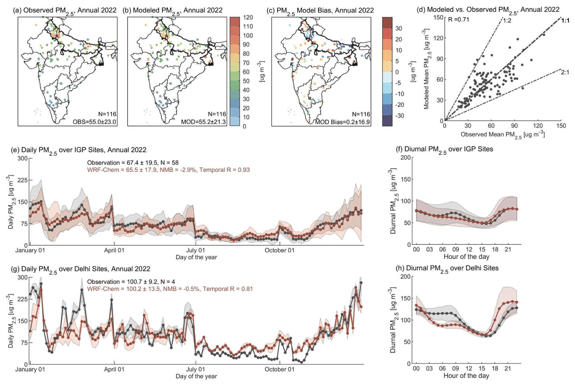
Figure 3 Comparison of observed and modeled surface PM_2.5 concentrations in 2022. Measurement stations with at least 80 % valid hourly data during the four-month period (January, April, July, and October) are selected. Multiple measurements within a single WRF-Chem grid cell are averaged before comparison with WRF-Chem. (a)–(d), comparison of annual mean surface PM_2.5 concentrations between observations (OBS) and model simulations (MOD). Annual value is estimated by averaging PM_2.5 concentrations during the four-month period. In (a)–(c), N denotes the number of grid cells used for evaluation, and the other numbers represent the mean ± one standard deviation across all grid cells. The thick black line denotes the boundary of the Indo-Gangetic Plain (IGP). In (d), R is the Pearson correlation coefficient between observed and modeled annual mean concentrations across all grid cells. (e) and (g), comparison of daily mean surface PM_2.5 concentrations between observations and WRF-Chem simulations in the IGP (e) and Delhi (g). (f) and (h) are the same as (e) and (g), but for annual mean PM_2.5 diurnal variations. In (e)–(h), red and black lines represent PM_2.5 concentrations for observations and simulations, respectively, averaged across available grid cells in each region noted in the panel, with shaded areas indicating one standard deviation. Temporal R is the Pearson correlation coefficient between the red and black lines in each panel. See Table S4 for PM_2.5 model performance at state level. See Fig. S2 for a scatter plot of daily modeled versus observed PM_2.5 for all valid grid-day pairs and a map of grid-level temporal Pearson correlation coefficients (R) for daily PM_2.5.

Beyond annual averages, WRF-Chem also effectively captures daily PM_2.5 variations throughout the four-month period (Fig. 3e–h). In the IGP and Delhi, the Pearson correlation coefficients between modeled and observed regional mean daily PM_2.5 concentrations are 0.93 and 0.81, respectively. In addition, the twin-peak pattern in diurnal PM_2.5 concentrations are well reproduced by WRF-Chem, though the morning peak in Delhi is underestimated. In contrast, model simulations without the emission and near-surface mixing updates show much stronger diurnal variability in hourly PM_2.5 concentrations than the observation, resulting from overestimated local emission fluxes and insufficient nighttime near-surface mixing (Fig. 4).

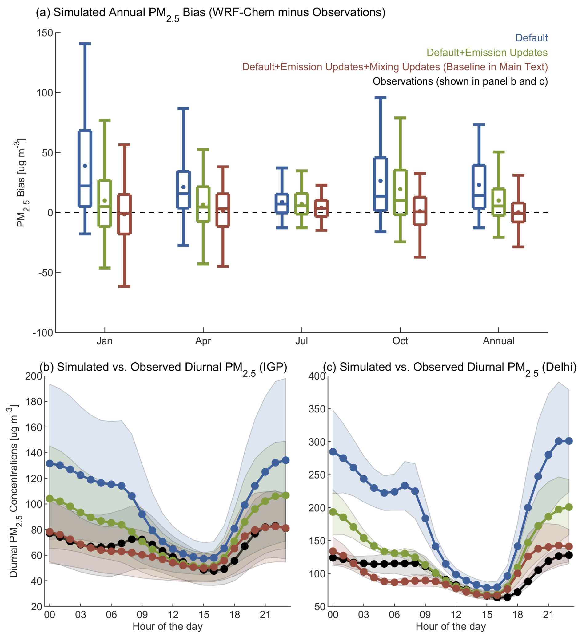
Figure 4 Comparison of PM_2.5 performances among three emission and model configurations in 2022. The configurations are: (1) Default (in blue) – official WRF-Chem v4.6.1 with the GEOS-Chem simple SOA scheme, driven by the standard CEDS and EDGAR inventories as described in Sect. 2.2.1; (2) Default + Emission Updates (in green) – configuration (1) plus sectoral updates for the residential and power sectors, as well as road dust, as described in Sect. 2.2.1 and 2.2.2; (3) Default + Emission Updates + Mixing Updates (in red) – configuration (2) plus improved near-surface mixing of chemical species, this configuration is adopted in the Baseline simulation as mentioned in Table 1 and Figs. 3 and 5. Model performance is evaluated using (a) monthly and annual mean bias across the entire domain, and (b–c) annual mean PM_2.5 diurnal patterns for the Indo-Gangetic Plain (IGP) and Delhi, respectively. In (a), box-whisker plots demonstrate the distribution of PM_2.5 model bias across the entire domain simulated by three configurations. The boxes denote the 25th, 50th, and 75th percentiles, and the whiskers denote the 5th and 95th percentiles of PM_2.5 bias. In (b)–(c), shaded areas indicate one standard deviation across available grid cells in each region noted in the panel.

Despite the good model performance of the baseline simulation discussed above, notable biases remain in several regions (Fig. 3b). Specifically, modeled annual mean surface PM_2.5 concentrations exceed observations by more than 30 µg m⁻³ in West Bengal (e.g., Kolkata) and a few stations in Gujarat, Punjab, and Rajasthan, while modeled concentrations underestimate observations by more than 30 µg m⁻³ in a few stations in Bihar and Uttar Pradesh. We summarize the state-level model performance in Table S4. We find the largest negative model bias in annual mean surface PM_2.5 concentrations in Bihar ($-\mathrm{19}\pm \mathrm{12}$ µg m⁻³, $-\mathrm{23}\pm \mathrm{17}$ %). In contrast, the largest positive model bias occurs in West Bengal, where modeled annual mean surface PM_2.5 concentrations exceed observations by 32±19 µg m⁻³ (61±47 %). Model biases in January play a dominant role in these annual biases, contributing, on average, 51 % (10 µg m⁻³) of the annual negative bias in Bihar and 57 % (18 µg m⁻³) of the annual positive bias in West Bengal. PM_2.5 concentrations observed at CPCB stations in Kolkata (West Bengal) are systematically lower compared to those recorded at the nearby US Air Now station, by 60 µg m⁻³ (39 %) in January and 30 µg m⁻³ (44 %) annually. A model evaluation at Kolkata using only the US Air Now station data, instead of averaging across all available measurement stations, significantly reduces the positive model bias from 145 % to 49 % in January, and from 147 % to 45 % annually.

We then utilize satellite-derived AOD data to evaluate the model's performance in simulating the spatial distribution of aerosol column loadings across India. Satellite data provides greater spatial coverage than the surface PM_2.5 measurement network. WRF-Chem reproduces the spatial pattern of AOD, with a Pearson correlation coefficient of 0.84 between annual modeled and observed AOD across India, and monthly correlations ranging from 0.72 to 0.82 (except for July when too much data is missing) (Fig. S3). However, WRF-Chem exhibits a consistent negative bias in AOD across India, with an annual mean bias (normalized mean bias) of $-\mathrm{0.12}\pm \mathrm{0.06}$ ($-\mathrm{29}\pm \mathrm{14}$ %) compared to satellite observations. AOD underestimation persists even in regions where surface PM_2.5 concentrations are significantly overestimated (e.g., West Bengal). Evaluation of daily AOD model values demonstrates that while the model performs well in capturing general AOD trends throughout the year, it fails to reproduce the magnitude of extreme AOD events over Delhi and the IGP. Previous modeling studies have attributed similar AOD underestimation over India primarily to the underrepresentation of large particles (diameter >2.5 µm) (David et al., 2018; Singh et al., 2021). Consistent with this, our baseline simulation underestimates annual mean surface coarse particulate matter (PM_coarse) by 37.3±25.7 µg m⁻³ (59±41 %) compared to CPCB measurements (Fig. S4). Additional discussion regarding missing PM_2.5 emissions and other factors contributing to the AOD bias is provided in Sect. S2.2 in the Supplement.

3.3 Total surface PM_2.5 concentrations and their source attribution across India in 2022

We analyze the national and regional surface PM_2.5 concentrations (both total and attributed to specific sources) using the PW mean metric (see Sect. 2.2.3 for PW mean calculation). PW mean concentrations reflect population exposure and is indicative of associated health risks. In addition, we investigate the spatial distribution of PM_2.5 concentrations originating from various sources in order to identify local hotspots associated with specific emission sources.

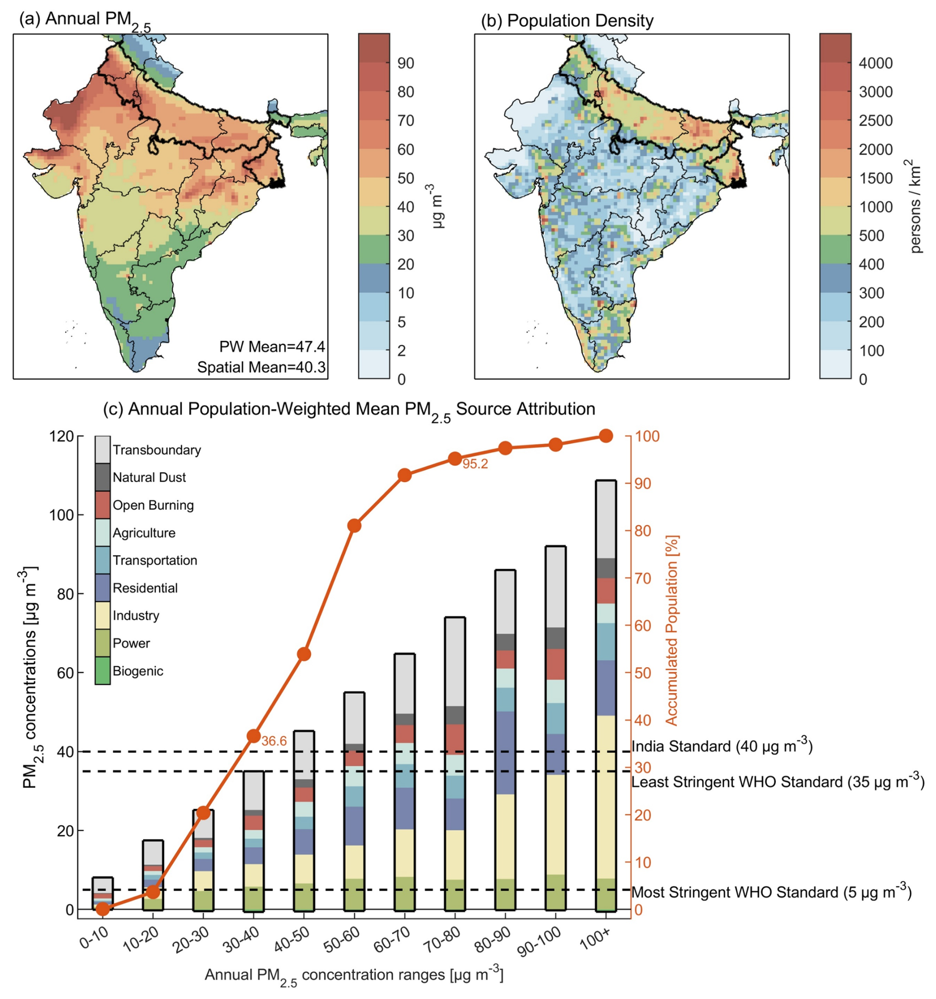
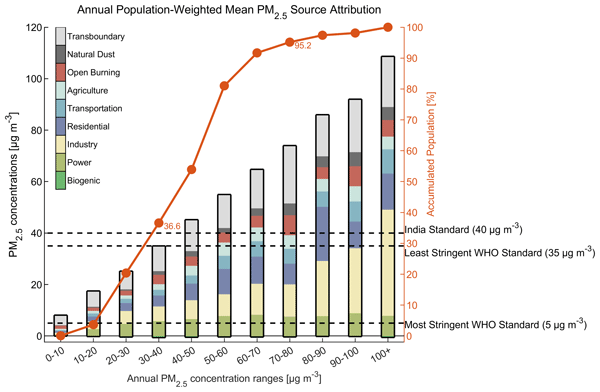
Figure 5 Baseline annual PM_2.5 concentrations in 2022 across India and their source attribution. In (a), Annual results are calculated as the average of January, April, July, and October simulations. Spatial distribution of annual average PM_2.5 concentrations across India are shown in color. National averages for Population-Weighted (PW) and spatial mean PM_2.5 concentrations are given as inset values in the figure. Panel b shows gridded population density across India. In (a) and (b), the thick black line denotes the boundary of the Indo-Gangetic Plain (IGP). In (c), WRF-Chem grids are aggregated by ranges of annual mean PM_2.5 concentrations, with colored bars indicating source attribution (left y axis). The red line and dots indicate the cumulative percentage of the population (right y axis) living in areas where the annual mean PM_2.5 concentration falls within or below a given concentration range. For example, 36.6 % (95.2 %) of the Indian population was exposed to annual PM_2.5 concentrations <40 (80) µg m⁻³ in 2022. See monthly versions of panel (c) in Fig. S5.

Our WRF-Chem simulation estimates a 2022 national PW mean annual surface PM_2.5 concentration of 47.4 µg m⁻³ (Fig. 5a), similar to the 51.6 µg m⁻³ reported in a recent satellite-based machine learning study (Kawano et al., 2025). In 2022, 37 % of India's population lived in areas where annual PM_2.5 concentrations met the national air quality standard of 40 µg m⁻³ (Fig. 5c), representing an increase from 17 % in 2016 (Apte and Pant, 2019). This change indicates an improvement in India's PM_2.5 air quality from 2016 to 2022 under the NCAP, aided by favorable meteorological conditions that enhanced pollutant dispersion and removal (Xie et al., 2024). However, in 2022, only 29 % of the national population was exposed to PM_2.5 levels below the least stringent annual World Health Organization (WHO) standard (35 µg m⁻³), and less than 0.1 % met the most stringent annual WHO standard (5 µg m⁻³). Regionally, the IGP experienced the highest annual PW mean PM_2.5 concentration in 2022 at 58.9 µg m⁻³, followed by Northwest India (58.3 µg m⁻³) and Central India (46.3 µg m⁻³). In contrast, Northeast India (28.1 µg m⁻³), South India (27.3 µg m⁻³) and the Himalayan states (25.3 µg m⁻³) had lower annual PW mean PM_2.5 concentrations.

At the national level, emissions originating within India accounted for 73 % (34.5 µg m⁻³) of the annual PW mean PM_2.5 concentration in 2022, while transboundary emission sources contributed the remaining 27 % (12.8 µg m⁻³) (Fig. 6). We summarize the national and state-level PW mean PM_2.5 concentrations attributed by source in Table S5.

Among domestic sources, the industrial sector was the leading contributor to the national annual PW mean PM_2.5 concentration in 2022, accounting for 18 % (8.6 µg m⁻³). Spatially, its contribution was particularly dominant in heavily polluted areas where annual PM_2.5 levels exceeding 80 µg m⁻³ (twice the national standard) (Fig. 5c). In some local hotspots within these areas, including major urban centers such as those of Delhi and Mumbai, industrial emissions alone contributed more than 40 µg m⁻³ to simulated annual surface PM_2.5 concentrations (Fig. 6), suggesting that to achieve national air quality standards in these hotspots it will be necessary to regulate industrial emissions.

India's residential sector, which has been undergoing a clean energy transition toward LPG since 2016, was the second-largest domestic contributor (15 %; 7.3 µg m⁻³) to the national PW mean PM_2.5 concentration in 2022. Spatially, however, the residential sector remained the dominant PM_2.5 source across large areas of the IGP, especially during winter (Fig. 7). Consequently, ∼500 million people in India lived in areas where residential emissions were the dominant source of annual PM_2.5 pollution in 2022, the highest among all emission sectors within India. This highlights the continued substantial health burden associated with residential emissions, and the need to augment recent progress in adoption of cleaner cooking fuels.

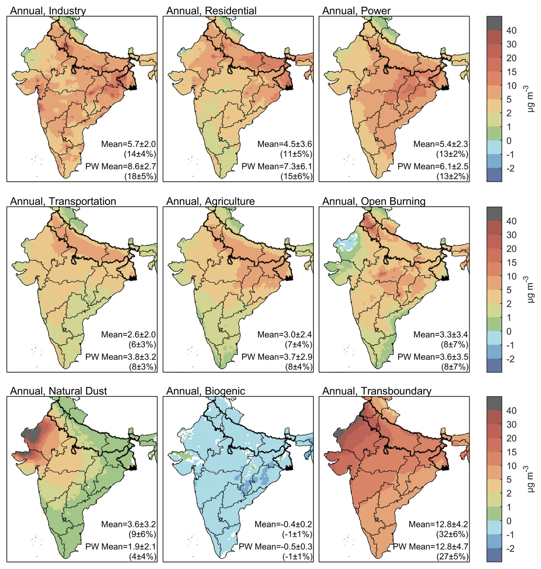
Figure 6 Spatial pattern of annual surface PM_2.5 concentrations across India in 2022 attributed to a given source. Annual results are calculated as the average of January, April, July, and October simulations. In each panel, numbers outside parentheses indicate the annual Population-Weighted (PW) mean PM_2.5 concentrations and spatial mean (Mean) PM_2.5 concentrations across India. Numbers inside parentheses represent the source's percentage contribution across India to total PM_2.5. Uncertainty bounds represent one standard deviation across monthly values, and provide an indication of the seasonal variation of a given sector's impact on surface PM_2.5. See Table S5 for source contribution to annual PW mean PM_2.5 at each state. The thick black line denotes the boundary of the Indo-Gangetic Plain (IGP).

India's power sector, based on our updated emission inventory, was the third-largest domestic contributor to the national PW mean PM_2.5 concentration in 2022 (13 %; 6.1 µg m⁻³). Spatially, the power sector primarily influenced PM_2.5 air quality in Central India, particularly in Chhattisgarh and Jharkhand (Figs. 6 and 7). This is due to central India generating 52 % of India's annual coal-based electricity in 2022 and power plants typically having emission controls only on primary particulates and not on SO₂ or NO_x which contribute to the formation of secondary inorganic aerosols.

India's transportation sector made a smaller contribution to the national annual PW mean PM_2.5 concentration in 2022 (8 %; 3.8 µg m⁻³), compared with the industry, residential, and power sectors. Spatially, its impact was most notable across much of the IGP and eastern Rajasthan, where it contributed moderately (∼5 to 10 µg m⁻³) to annual PM_2.5 (Fig. 5). In Delhi, the transportation sector recorded its highest state-level contribution to annual PM_2.5, reaching 11.6 µg m⁻³ (11 %, Table S5). However, transportation was not the dominant domestic source of annual PM_2.5 in any of India's populous regions in 2022 (Fig. 7).

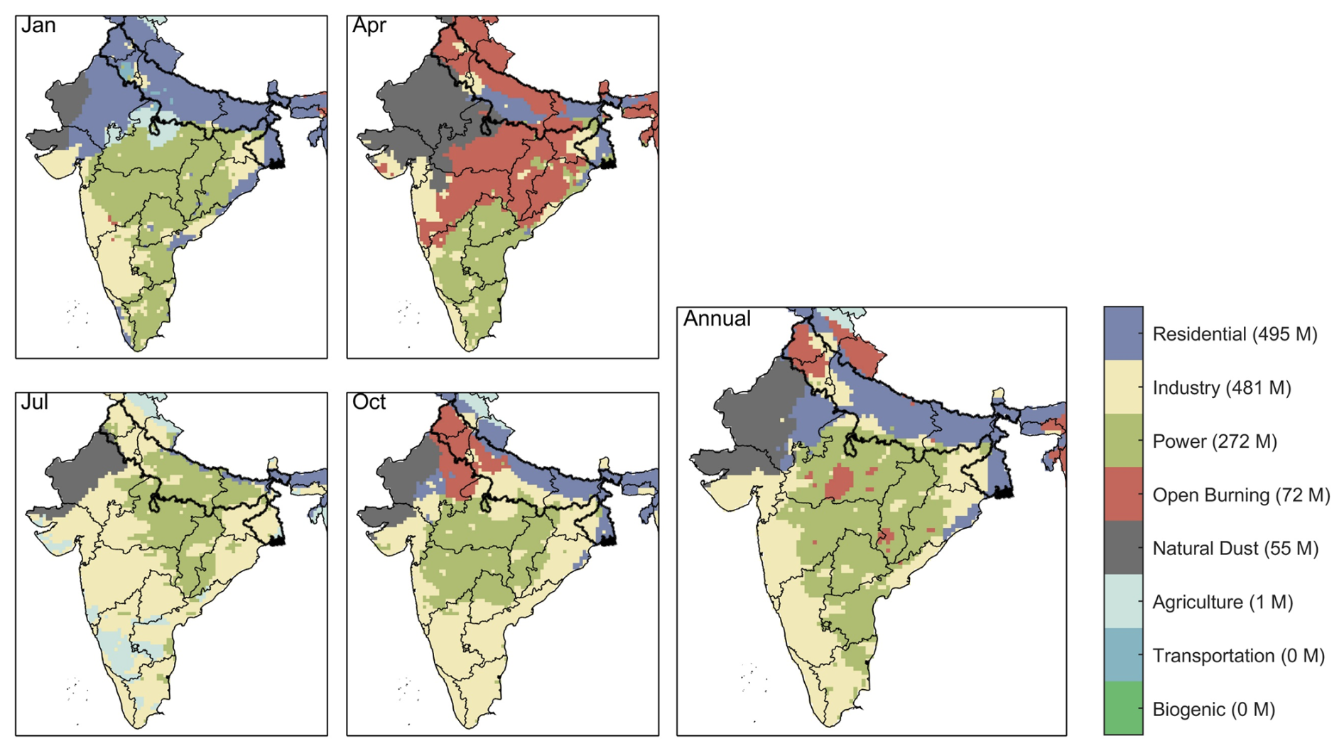
Figure 7 Dominant domestic PM_2.5 sources at monthly and annual timescales. Transboundary emission sources are excluded. Numbers in parentheses in the legend indicate the population (in millions) across India living in areas where a specific domestic emission source dominated in 2022. The thick black line denotes the boundary of the Indo-Gangetic Plain (IGP).

India's agricultural sources contributed 8 % (3.7 µg m⁻³) to the national annual PW mean PM_2.5 concentration. This PM_2.5 was primarily derived from secondary inorganic aerosols formed from NH₃ emitted from fertilizer use and livestock as well as a minor source from NO_x emitted from agricultural fields.

India's open burning emissions, derived from the FINN inventory and representing satellite-detectable burning of crop residues, municipal waste and wildfires, contributed 8 % (3.6 µg m⁻³) to the annual PW mean PM_2.5 concentrations across India in 2022. Their impacts were strongly seasonal, with elevated contributions of 15 % (8.3 µg m⁻³) and 10 % (4.3 µg m⁻³) to the national PW mean PM_2.5 in April and October, respectively. Spatially, the regional hotspots switched between months. In April, open burning is most influential in Central India and Northeast India (Fig. 7). In October, open burning became the dominant source of PM_2.5 in northeastern IGP, including Delhi, with significant monthly contributions by ∼27 µg m⁻³ (Fig. S6). Previous studies have shown that groundwater conservation policies in the northeastern IGP (one of India's major crop harvesting and residue burning regions) have shortened the turnover period between crop seasons and delayed agricultural burning. As a result, burning has shifted later in the year, often extending into late fall, when meteorological conditions are less favorable for pollutant dispersion, thereby amplifying the impact of open burning on surface PM_2.5 concentrations (Liu et al., 2022). These earlier findings underscore the complexity of effectively controlling open burning emissions.

India's natural dust emissions, derived from desert dust simulated by WRF-Chem, contributed 4 % (1.9 µg m⁻³) to the national annual PW mean PM_2.5 concentration in 2022. Spatially, it had a substantial impact on PM_2.5 levels in Northwest India, where grid-level annual contributions exceed 40 µg m⁻³ in its western part. However, due to the low population density in Northwest India and the limited impact of natural dust on surface PM_2.5 outside this region (Figs. 5b and 6), natural dust was not a major factor for PM_2.5 exposure at the national level. Despite limited exposure among the population, the natural dust zones overlap substantially with India's solar energy generation centers. This spatial coincidence may lower solar power generation efficiency due to aerosol-induced dimming and soiling, though the soiling impact can be mitigated if panels are cleaned on a regular basis (Li et al., 2020).

India's biogenic emissions had a small but net negative contribution to annual PW mean PM_2.5 concentrations across the country (−1 %; −0.5 µg m⁻³). Biogenic emissions contribute to OA formation, but in our simulations, the OA concentration increase (<0.1 µg m⁻³) is outweighed by secondary inorganic PM_2.5 concentration decrease (−0.5 µg m⁻³) when biogenic emissions are included. We find a reduction in all secondary inorganic PM_2.5 components (i.e., sulfate, nitrate, and ammonium), as well as in the sulfate oxidation ratio and nitrate oxidation ratio, following the inclusion of India's biogenic emissions (Fig. S7). Biogenic VOCs reduced the oxidation capacity of the atmosphere by consuming OH and HO₂ radicals, thereby decreasing the conversion of SO₂ to sulfate and NO₂ to nitrate, which also reduced ammonium formation and led to reductions in secondary inorganic PM_2.5. Consequently, biogenic emissions from within India resulted in a slight net reduction in total PM_2.5 concentrations in 2022. However, they significantly enhanced annual mean O₃ concentrations (by up to 20 µg m⁻³, Fig. S7), deteriorating O₃ air quality across India.

Transboundary sources (emissions from outside of India) accounted for 27 % (12.8 µg m⁻³) of annual national PW mean PM_2.5 in India in 2022, exceeding the contribution of any individual domestic emission source (Fig. 6). These transboundary sources include emissions from six anthropogenic sectors (i.e., power, industry, residential, transportation, agriculture, and open burning) and two natural sources (i.e., dust and biogenic) from outside India, representing emissions beyond the jurisdiction of the Indian government. Spatially, the influence of transboundary sources exhibits a northwest-to-southeast gradient. In 2022, transboundary sources contributed more than 20 % to grid-level annual PM_2.5 concentrations across most of India, with contributions exceeding 40 % in western states such as Punjab, Haryana, Rajasthan, and Gujarat (Fig. S8). In Delhi, transboundary sources contributed 20 % (21 µg m⁻³) to the annual PM_2.5 concentration in 2022. Further decomposition reveals that anthropogenic emissions originating from neighboring countries within our modeling domain accounted for 11 % (5.2 µg m⁻³) of the 2022 annual national PW mean PM_2.5 in India. Meanwhile, other transboundary components, comprising regional natural sources (dust and biogenic) and long-range transport of pollutants entering via model lateral boundary conditions, contributed the remaining 16 % (7.7 µg m⁻³) (Fig. S9).

3.4 Chemical components of total surface PM_2.5 and their source attribution across India for 2022

We analyze the contributions of individual PM_2.5 components simulated by WRF-Chem to total PM_2.5 concentrations across India in 2022, along with their respective source attributions. Figure 8 shows the spatial distribution of annual concentrations of all components. Figure 9 and Table S6 present the source contributions to national PW mean concentrations of PM_2.5 components.

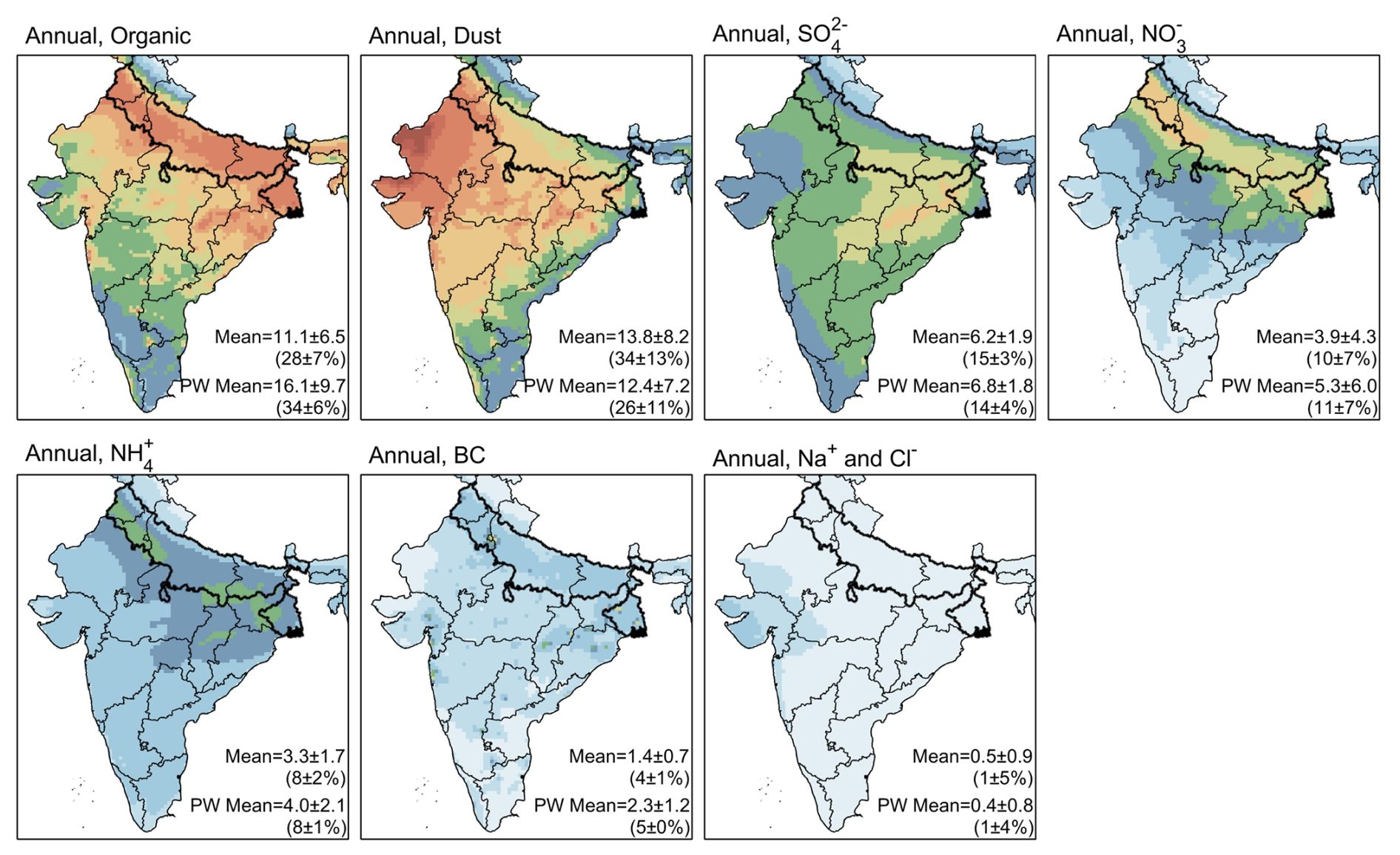
Figure 8 Spatial pattern of annual concentrations of PM_2.5 components across India in 2022. Annual results are calculated as the average of January, April, July, and October simulations. In each panel, numbers outside parentheses indicate the Population-Weighted (PW) mean concentrations and spatial mean (Mean) concentrations across India. Numbers inside parentheses represent the component's percentage contribution to total PM_2.5. Uncertainty bounds represent one standard deviation across four monthly values representing each season. The thick black line denotes the boundary of the Indo-Gangetic Plain (IGP).

Among components resolved by WRF-Chem, organic aerosols (including both primary and secondary) had the largest contribution to the national PW mean total PM_2.5 concentrations in 2022, at 34 % (16.1 µg m⁻³) (Fig. 8). Residential emissions from within India were the dominant source of population exposure to organic PM_2.5, accounting for 6.6 µg m⁻³ of its annual national PW mean concentration (Fig. 9). Transboundary (3.1 µg m⁻³) and industrial (2.6 µg m⁻³) sources were also significant contributors to organic PM_2.5 levels across the country. Spatially, organic PM_2.5 had a north-to-south gradient, with its dominance closely overlapping with regions where residential emissions were also dominant, particularly the IGP.

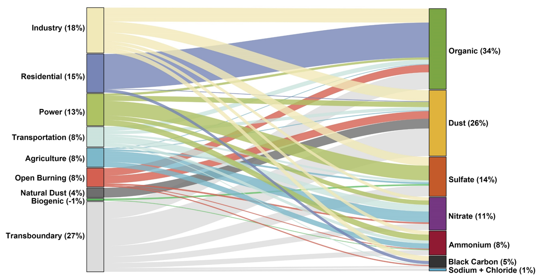
Figure 9 Source contributions to population-weighted mean concentrations of PM_2.5 components across India in 2022. Contributions are attributed to six domestic anthropogenic sectors (industry, residential, power, transportation, open burning, and agriculture), two domestic natural sources (dust and biogenic emissions), as well as sources from outside of India (transboundary emissions). Note that contributions below 0.1 µg m⁻³ for a given source–component pair are omitted from the figure. All contributions presented are positive, except those from biogenic sources, which are negative. Numbers in parentheses indicate the percentage share (rounded to the nearest integer) of each source or component in the total PM_2.5 concentration. See Table S6 for detailed values for each pair in this figure.

The dust component, including both anthropogenic and natural sources, was the second-largest contributor to the national PW mean total PM_2.5 concentration in 2022, at 26 % (12.4 µg m⁻³) (Fig. 8). Transboundary emissions dominated dust PM_2.5 at the national level, contributing 5.0 µg m⁻³ to its annual PW mean concentration (Fig. 9). In addition, industrial (2.0 µg m⁻³) and natural dust (1.8 µg m⁻³) emissions from within India were the other major contributors to dust PM_2.5 across India. Spatially, dust PM_2.5 exhibited a west-to-east gradient, with annual concentrations exceeding 40 µg m⁻³ across most of Rajasthan and Gujarat (Fig. 8).

Sulfate PM_2.5 was the third-largest contributor to the national PW mean total PM_2.5 level in 2022, at 14 % (6.8 µg m⁻³), and was the dominant component of secondary inorganic PM_2.5 (including sulfate, nitrate, and ammonium) (Fig. 8). India's power sector, the largest domestic SO₂ emitter, was the dominant source for sulfate, accounting for 2.8 µg m⁻³ of its annual PW mean concentration, followed by transboundary pollution and the industrial sector (Fig. 9). Spatially, sulfate concentrations exhibited a relatively small gradient compared to organic and dust PM_2.5, though highest concentrations were found in Central India around Chhattisgarh and Jharkhand.

Nitrate PM_2.5 contributed 5.3 µg m⁻³ (11 %) to national PW mean total PM_2.5 concentration in 2022, smaller than that of sulfate PM_2.5 (Fig. 8). However, spatially nitrate PM_2.5 was the dominant component among secondary inorganic PM_2.5 across the IGP, especially in Bihar, Haryana, and Delhi. Unlike organic, dust, and sulfate PM_2.5, nitrate PM_2.5 exhibited highly nonlinear relationships between precursor (i.e., NO_x) emissions and resulting concentrations. Specifically, the agriculture sector, which contributed only 2 % of national NO_x but 80 % of national NH₃ emissions in 2022, were identified as the largest contributor (2.0 µg m⁻³) to nitrate PM_2.5 in 2022 (Fig. 9). In the atmosphere, nitric acid (HNO₃, from NO_x oxidation) reacts with NH₃ remaining after neutralizing sulfuric acid to form ammonium nitrate. Removing agricultural emissions reduced NH₃ availability across India by 77 %, cutting the national average NO${}_{\mathrm{3}}^{-}$ fraction of total NO${}_{\mathrm{3}}^{-}+$ HNO₃ from 51 % (baseline) to 25 % and leading to the largest nitrate reduction among all simulations that removed individual sources (Fig. 10).

Ammonium PM_2.5 contributed 4.0 µg m⁻³ (8 %) to national PW mean total PM_2.5 concentration in 2022, with spatial hotspots overlapping those of sulfate and nitrate (Fig. 8). Like nitrate, ammonium's response to precursor (NH₃) emissions was highly nonlinear. Notably, we identified India's power sector as the largest contributor (1.1 µg m⁻³) to ammonium PM_2.5 using the zero-out emission method (Fig. 9). While the power sector did not emit NH₃ directly, its dominance in SO₂ and NO_x emissions within India increased the availability of sulfuric and nitric acids, which react with NH₃ to form ammonium aerosols. Removing power sector emissions therefore left a larger fraction of total reduced nitrogen (NH_x= NH₃+ NH${}_{\mathrm{4}}^{+}$) as NH₃, leading to greater reductions in ammonium PM_2.5 than any other single-source removal scenarios (Fig. 10). In contrast, when removing agricultural emissions (dominant NH₃ source domestically), transport of NH₃ from outside India partially offset the decrease in NH₃ supply, sustaining some ammonium formation and leading to smaller reductions in ammonium than the simulation in which power-sector emissions were removed. These findings illustrate how non-linear chemistry, when source emissions are entirely removed, can yield results that deviate from those of attributional methods (e.g., tagging precursor emissions) (Koo et al., 2009).

Black Carbon, primarily from the incomplete combustion of solid fuels, contributed 2.3 µg m⁻³ (5 %) to national PW mean total PM_2.5 concentration in 2022, with India's industrial sector the dominant source.

Sodium and chloride together contributed only 0.4 µg m⁻³ (1 %) to national PW mean total PM_2.5 concentration in 2022, primarily from transboundary sources. Previous observational studies reported relatively high chloride concentrations in particulate matter in Delhi (e.g., 15-month average of 8.6 µg m⁻³ during 2017–2018), Kanpur (e.g., monthly average of 19.3 µg m⁻³ in January 2016), and Chennai (episodically), suggesting possible local emissions of hydrochloric acid from plastic-contained waste burning and industry (Gani et al., 2019; Thamban et al., 2019; Gunthe et al., 2021). However, because the emission inventories used in this study (i.e., CEDS, EDGAR, and FINN) do not include anthropogenic emissions of chloride-containing species, such elevated chloride levels observed in these cities were not reproduced in our model simulations. A recent modeling study that incorporated anthropogenic chlorine emissions reported a spatial average increase of 3–4 µg m⁻³ in PM_2.5 concentrations in the IGP during January–March 2018 (Patel et al., 2024). By comparison, our model simulated a spatial average of 88 µg m⁻³ for January 2022 and 56 µg m⁻³ for the annual mean in 2022 across the IGP, which suggests a relatively small impact of incorporating chlorine emissions into our source attribution studies.

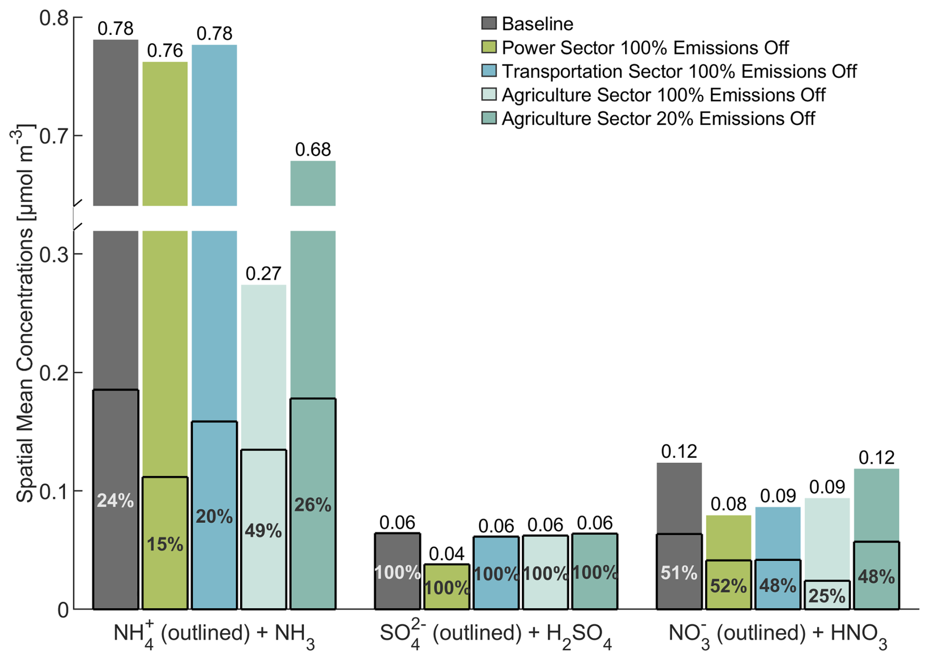
Figure 10 Partitioning between secondary PM_2.5 components (NH${}_{\mathrm{4}}^{+}$, SO${}_{\mathrm{4}}^{\mathrm{2}-}$, and NO${}_{\mathrm{3}}^{-}$) and their relevant precursors (NH₃, H₂SO₄ and HNO₃) for the baseline simulation and following the removal of individual sectoral emissions. Annual spatial mean concentrations (in µmol m⁻³) across India in 2022 are shown for the baseline simulation (grey bars) and for scenarios where individual sector emissions (power, transportation, and agriculture) are removed completely or reduced by 20 %. Solid-line-outlined boxes indicate the concentrations of NH${}_{\mathrm{4}}^{+}$, SO${}_{\mathrm{4}}^{\mathrm{2}-}$, and NO${}_{\mathrm{3}}^{-}$ aerosol particles, while the upper portions of each bar (above the outlined boxes) represent the concentrations of NH₃, H₂SO₄, and HNO₃. Numbers above each bar show the total concentration of the species group on the x-axis for the respective scenario. Percentages inside each outlined box indicate the share of NH${}_{\mathrm{4}}^{+}$, SO${}_{\mathrm{4}}^{\mathrm{2}-}$, and NO${}_{\mathrm{3}}^{-}$ in the total concentration of NH${}_{\mathrm{4}}^{+}+$NH₃, SO${}_{\mathrm{4}}^{\mathrm{2}-}+$H₂SO₄, and NO${}_{\mathrm{3}}^{-}+$HNO₃, respectively.

4 Discussion

India's residential sector has undergone an energy transition with part of the sector moving from inefficient solid fuels to cleaner LPG, resulting in substantial reductions in primary PM_2.5 emissions that would otherwise arise from biomass burning. The Pradhan Mantri Ujjwala Yojana (PMUY) program, launched in 2016, has played a central role by providing income support for LPG connections to rural and low-income households, and by December 2024 had reached over 103 million beneficiaries. Incorporating an updated residential inventory that captured this trend is key to our finding that the absolute and relative contributions of residential emissions to national population-weighted mean PM_2.5 concentration are smaller than in two earlier studies for 2016 (Singh et al., 2021; Pai et al., 2022) (Table 2), though it remained the leading domestic PM_2.5 source in the IGP (Fig. 11). In addition, our explicit separation of emissions from within and outside India further explains why our estimated residential contribution is smaller than in previous studies, which included transboundary residential sources when accounting for this sector (Conibear et al., 2018; Guo et al., 2018; Reddington et al., 2019; Chatterjee et al., 2023). However, recent research highlights challenges in sustaining LPG usage under PMUY, including high refill costs and subsidy delays (Asharaf and Tol, 2024; Gaikwad et al., 2025), which may result in backsliding to a continued reliance on solid fuels which may not be fully captured in the updated inventory.

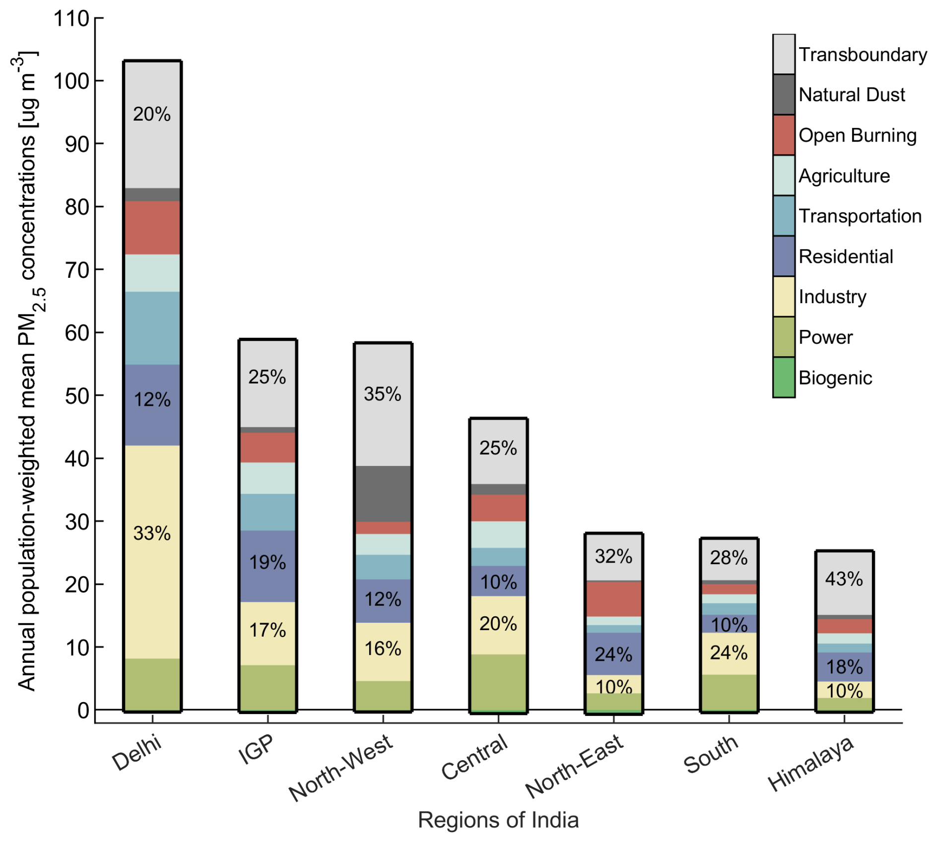
Figure 11 Source attribution of regional population-weighted mean annual PM_2.5 concentrations in 2022 across Delhi and six regions of India. Inset numbers illustrate the percentage contribution from the largest three sources (including the transboundary source) in each region.

India's industrial sector emerged as the largest domestic contributor to India's PM_2.5 pollution in 2022, resulting from rapid growth in activity and limited pollution controls. Specifically, its energy consumption nearly doubled from 7.8 EJ in 2010 to 13.6 EJ in 2022 with coal, biofuels, and waste being the dominant sources of energy (International Energy Agency, 2024), while emission regulations in this sector have primarily focused on improved energy efficiency with few new regulations focused on certain small-scale informal industries such as brick kilns (Ganguly et al., 2020; Tibrewal and Venkataraman, 2021). Consistent with these trends, the EDGAR global inventory reports an increase in primary PM_2.5 emissions from the industrial sector from 1.4 Tg yr⁻¹ in 2010 to 2.1 Tg yr⁻¹ in 2022. Our adoption of the EDGAR 2022 inventory for the industrial sector therefore results in higher estimated absolute and relative industrial contributions to national population-weighted mean PM_2.5 concentrations compared with earlier studies that focused on 2016 (Table 2). Notably, industrial sources contributed 33 % of Delhi's annual PM_2.5 in our analysis (Fig. 11), a sharp increase from 14 % in 2016 (Singh et al., 2021), underscoring the growing dominance of this sector in urban and national pollution burdens.

Table 2 A comparison of source attribution to national population-weighted mean PM_2.5 concentration in India across studies^a.

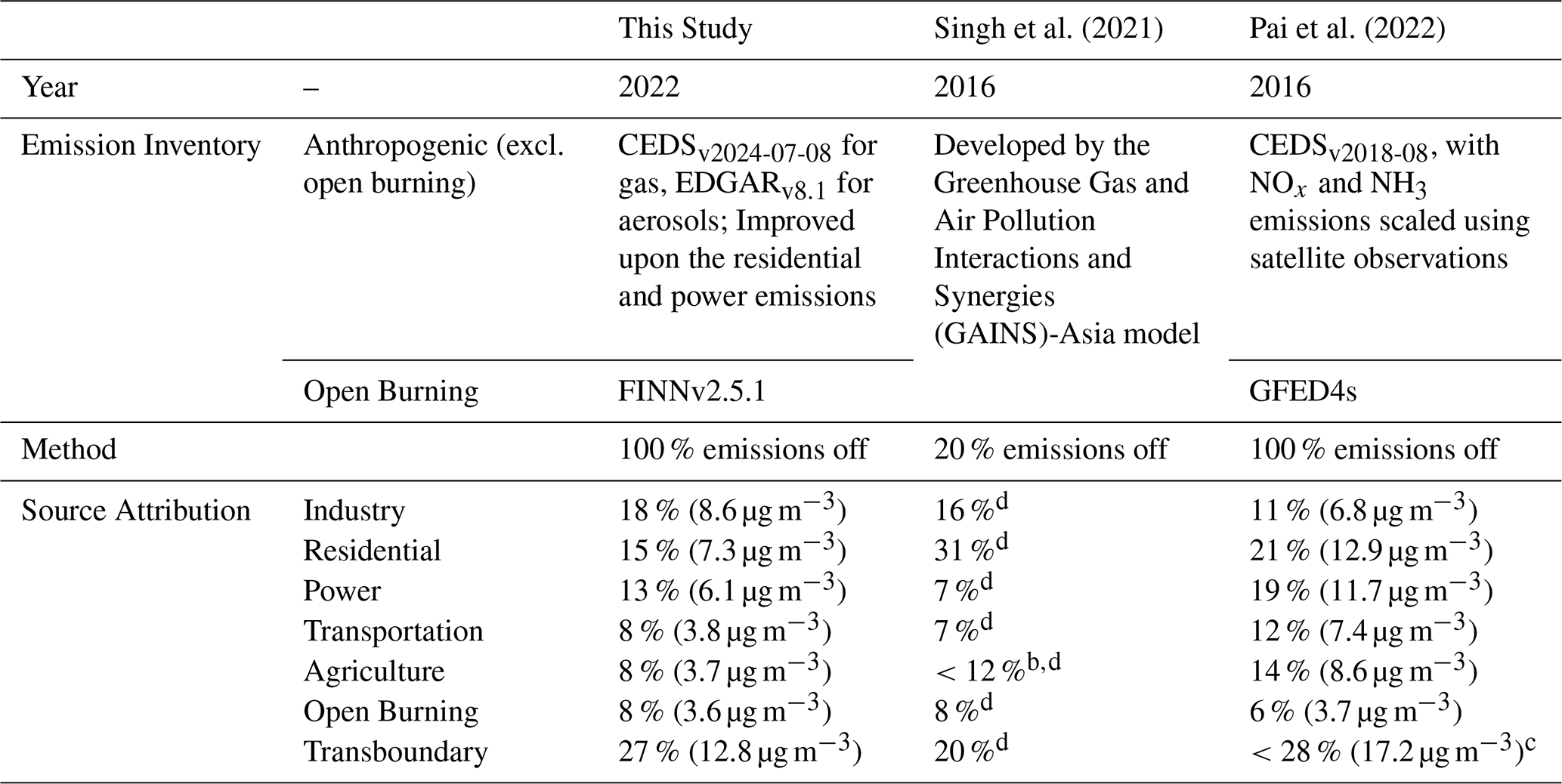
^a In this table, we only include studies that investigated emissions from within India for a direct comparison with our results. ^b Agricultural NH₃ emissions were aggregated with other emission source as “Others Source” in this study. ^c Transboundary sources were aggregated with natural emissions as “Background Source” in this study. ^d This study did not report national population-weighted mean PM_2.5 concentration attributed to a given source.

India's power sector has been heavily and increasingly relied on coal generation, with the challenges of implementing emission controls for SO₂ and NO_x. Coal-based electricity generation substantially increased from 658 TWh in 2010 to 1307 TWh in 2022 (International Energy Agency, 2024). Although the Indian government introduced stringent emission standards for thermal power plants in 2015, compliance has been weak, with only about 3 % of coal-based plants having installed FGD systems by 2022 (National Environmental Engineering Research Institute, 2024). As a result, SO₂ emissions from the power sector increased substantially between 2010 and 2022, with CEDS reporting a 34 % rise and EDGAR a 71 % rise, consistent with satellite-derived SO₂ total column concentration trends across India during this period (Xie et al., 2024). In addition, the adoption of NO_x control technologies in India's coal-fired plants are being tested but are not yet commercially deployed as India's high-ash coals can adversely impact NO_x control systems (Wiatros-Motyka, 2019). Projections further suggest that with only limited adoption and operation of pollution-control technologies continuing, SO₂ emissions from the power sector could rise by nearly 500 % between 2020 and 2050 (Venkataraman et al., 2018). These trends, combined with the recent suggested relaxation of FGD requirements for coal plants (Koshy, 2025), will likely increase secondary inorganic aerosol formation and will threaten to undermine national efforts to reduce PM_2.5 pollution and protect public health. The plant-level database and emission inventory developed in this study provide a foundation to further evaluate the air quality and health benefits of a clean power transition for future studies.

Import of pollution across national borders (transboundary sources) continued to be responsible on average for over 20 % of surface PM_2.5 pollution in 2022, similar to findings from 2016 (Table 2). These results underscore the persistent influence of transported pollution on India's air quality.

5 Uncertainty and limitation

Our annual source attribution results are subject to input uncertainty from emission inventories. Focusing on the sectors with India-specific updates, we estimate annual national population-weighted mean PM_2.5 contributions of 6.1±1.1 µg m⁻³ for the power sector and 7.3±3.7 µg m⁻³ for the residential sector. These estimates account for uncertainties in activity data, emission factors, and residential fuel use (see Sect. S4 in the Supplement and Table S7 for detailed quantification). We do not quantify uncertainties for sectors relying on global inventories (CEDS, EDGAR, FINN) due to the lack of India-specific uncertainty estimates for air pollutants in these datasets. However, we note that the upper uncertainty bound of the residential sector contribution (11 µg m⁻³) exceeds the baseline estimate for the industrial sector (8.6 µg m⁻³). Consequently, while our central estimates identify India's industrial sector as the largest domestic PM_2.5 source in 2022, the definitive ranking of these top two sectors is sensitive to the unquantified uncertainties in the industrial emission inventory.

Our baseline emission inventory has limitations in capturing temporal variations of real-world emission patterns. While annual mean PM_2.5 concentrations at the regional scale are reasonably represented (Fig. 3a–b), the model cannot fully reproduce extreme daily episodes (Fig. 3e and g). The substantial spread in the density scatter plot of observed and simulated daily PM_2.5 concentrations at observed PM_2.5 values above 100 µg m⁻³ indicates larger model uncertainty during moderate-to-extreme pollution episodes, with a tendency to underestimate the magnitude of some high-pollution events, although both under- and overestimation occur (Fig. S2). This limitation partly stems from how temporal allocations of emissions are handled in our model: for anthropogenic sources, including industry, residential combustion, power generation, transport and agriculture, monthly totals are distributed evenly across days with prescribed sectoral diurnal profiles, smoothing episodic spikes (e.g., holidays and weather-driven activity changes). For biomass burning, we use the satellite-based FINN inventory at daily resolution, which better captures day-to-day variability; however, satellite-derived fire inventories can still underestimate emissions from small-scale fires or be degraded by cloud cover and thick haze during intense pollution episodes. Natural dust and biogenic emissions are calculated online within WRF-Chem using real-time meteorology, but carry uncertainties from static input parameters (e.g., land use type, surface erodibility, leaf area index) and biases in simulated meteorological fields (e.g., wind speed).

Using single months (January, April, July and October) to represent entire seasons may underrepresent the air quality impacts of episodic emission sources with strong intra-seasonal variability, such as open biomass burning and its transboundary transport. For example, post-monsoon crop-residue burning in northwestern India has shifted later in the season, with peak burning delayed into November (Sembhi et al., 2020; Liu et al., 2022). In addition, open biomass burning in Northeast India and adjacent regions, particularly Myanmar, is most active during the dry pre-monsoon period, with strong fire activity and emissions in March–April (Singh et al., 2020). Our seasonal sampling does not fully capture these episodic peaks (e.g., missing March and November), and the source attribution for open burning and its transboundary transport, particularly at the regional level, should therefore be considered conservative lower bounds.

Our source attribution approach has inherent limitations due to the nonlinear chemistry of secondary aerosol formation and aerosol–meteorology feedbacks, similar to previous studies that employed the complete source removal method (Conibear et al., 2018; Pai et al., 2022; Chatterjee et al., 2023). For example, we identify the power sector as the largest contributors to ammonium PM_2.5 in 2022, despite the fact that it did not emit NH₃. This result is primarily driven by secondary inorganic aerosol chemistry (discussed in Sect. 3.4) and are consistent with findings from a previous study for 2016 (Pai et al., 2022). We also find a small but non-negligible contribution of agricultural emissions to national PW mean dust concentrations (0.15 µg m⁻³). This counterintuitive result reflects the impact of aerosol–meteorology feedbacks: when agricultural emissions are removed, reductions in secondary PM_2.5 improve ventilation conditions by weakening aerosol–radiation interactions (Zhou et al., 2019), thereby lowering primary PM_2.5 concentrations, even though their emissions themselves are unaffected. These examples illustrate the interpretive challenges inherent to source attributional results via complete emission removal.

Nonlinear secondary aerosol chemistry limits the direct application of our results to real-world emission regulations, particularly for sources dominated by PM_2.5 precursor emissions whose reductions have a nonlinear effect on resulting PM_2.5 concentrations, since emission control policies typically require partial rather than complete reductions. To address this limitation, we conduct three additional simulations where we individually reduce emissions from industrial, residential, and agricultural sectors by 20 % (Table 1). For sources dominated by primary PM_2.5 components, such as the industrial and residential sectors, the differences between complete removal and scaled partial reductions are small at the national level: national spatial mean and population-weighted mean PM_2.5 concentration reductions differ by less than 7 % and 3 %, respectively, between a 100 % emission reduction and a fivefold scaling of 20 % reductions (Fig. S10). However, for the agricultural sector, a 20 % emission reduction results in a 25 % smaller reduction in national PM_2.5 concentrations (after a fivefold scaling) than a 100 % emission reduction. This nonlinearity is primarily due to India's overall NH₃-rich environment (Fig. 10), where nitrate availability limits secondary inorganic aerosol formation. This suggests that partial removal of NH₃ is less effective, defined as concentration decrease per unit emission reduction, in mitigating PM_2.5 than substantial NH₃ emission reductions, especially in northern India.

Finally, the qualitative attribution of AOD underestimation to missing coarse PM mass in the Sect. S2.2 in the Supplement should be interpreted as a diagnostic discussion of likely bias sources, not as a quantitative source apportionment of AOD. Given the non-linear relationship between surface aerosol mass and column-integrated AOD resulting from variations in aerosol composition and vertical profiles (Wang et al., 2021; Zhu et al., 2024), the mass-based surface PM_2.5 source attribution results presented in this study should not be directly extrapolated to infer source contributions to AOD or AOD bias.

6 Conclusion and Implications

We conduct the first WRF-Chem model evaluation and source attribution analysis for India for the year 2022, leveraging recent advances in India-specific residential and power sector emission inventories and the expansion of ground-based PM_2.5 monitoring networks. Our simulations incorporate the 2022 CEDS and EDGAR global emission inventories (released in 2024), a 2022 coal-fired power plant emission inventory developed in this work, and a revised 2022 residential emission inventory (Velamuri et al., 2024). We also incorporate the GEOS-Chem simple SOA scheme into WRF-Chem and improve model treatment of near-surface mixing of pollutants. We evaluate the baseline WRF-Chem simulation against observed PM_2.5 concentrations from 288 surface monitoring sites across India and neighboring countries, demonstrating very good model performance across India that captures spatial and temporal variations of PM_2.5 concentrations in 2022. Our findings, compared with earlier source attribution studies, highlight that residential emissions from within India are no longer the largest source of national population-weighted mean PM_2.5 pollution, although they remained the second-largest domestic contributor nationally (Figs. 6 and 9) and the leading contributor regionally in the Indo-Gangetic Plain (Fig. 11). Instead, industrial emissions from within India emerged as the largest domestic contributor at the national scale, while the power sector within India ranks third, with 77 % of its contribution arising from secondary inorganic PM_2.5 formed from gaseous precursor emissions. Importantly, transboundary sources contributed more than any individual domestic source to surface PM_2.5 concentrations in 2022 across India.

Tracking India's evolving air pollution and the shifting contributions of various sources is needed to inform regulatory mitigation strategies. This requires robust air quality modeling based on up-to-date emission inventories that incorporate real-world changes in activity, emission factors, technology adoption, and regulations. By combining information from both global and regional inventories, our study provides an improved understanding of PM_2.5 pollution and its source attribution for 2022, with several implications. First, efforts to reduce primary PM_2.5 emissions from the residential sector have been beneficial and should continue through initiatives such as the NCAP and the residential PMUY programs. In addition, electrification of the residential sector coupled with decarbonization of the grid can further help reduce air pollution emissions (Zhou et al., 2022). Second, enforcement of new stringent emission regulations targeting both primary PM_2.5 and SO₂ are needed for the fast-growing industrial sector, especially in densely populated urban areas. Continuing to improve energy efficiency for large and energy-intensive industries such as steel production under the Perform, Achieve, and Trade (PAT) scheme will also be beneficial for mitigating primary PM_2.5 and SO₂ emissions from the industrial sector (Ministry of Power, 2022). Third, SO₂ controls in the coal dominated power sector should be enforced to prevent further deterioration of air quality particularly as new coal power comes on-line. Finally, more stringent regulations of local emissions are needed in areas heavily influenced by transboundary pollution in order to meet air quality standards. Collaborative efforts, including data sharing and cross-border source identification between India and its neighboring countries would be beneficial in identifying opportunities to improve air quality within South Asia. Future Indian PM_2.5 pollution and its source attribution research will benefit from the development of a multiyear, India-specific emission inventory covering recent years to better support long-term air quality management.