Diurnal cycle of stratocumulus mesoscale convective cells in the South-East Pacific

Stratocumulus (StCu)-topped boundary layers exhibit complex mesoscale cellular convection that remains a primary source of climate radiative forcing uncertainty and a persistent challenge for models. While daytime snapshots have established a characteristic aspect ratio (AR) – the ratio of cell size λ to boundary-layer depth – of 30–40, its evolution over the full diurnal cycle remains poorly constrained. Here we use high-resolution infrared observations from GOES-East (2020–2025) over the South-East Pacific during August–September to provide a continuous day-to-night characterization of StCu spatial metrics. Using a brightness temperature difference framework ($\mathrm{\Delta }\text{Tb}={\text{Tb}}_{\mathrm{12.3}\mathrm{\mu }\mathrm{m}}-{\text{Tb}}_{\mathrm{10.3}\mathrm{\mu }\mathrm{m}}$), we reveal a robust, universal four-phase diurnal cycle: morning growth, early-afternoon plateau, rapid late-afternoon downscaling, and a stable nocturnal regime. We demonstrate a striking decoupling between metrics: while λ varies significantly across years, the AR curves collapse into a nearly identical diurnal signal across 2020–2025, filtering out interannual variability. However, this invariance is modulated by cloud-fraction regimes, controlling the cycle's amplitude and the timing of its growth and decay phases. This allows us to establish a nocturnal AR of about 25, with a transient daytime maximum of about 31. These typical values can be slightly sensitive to methodological choices, but in any case, the diurnal tendency remains the same. These results suggest a fundamental compensation between horizontal and vertical scales, with AR acting as a dynamical attractor of stratocumulus organization. Its persistence raises a key question: why is the mesoscale organization of stratocumulus so constrained?

1 Introduction

Marine boundary-layer (MBL) stratocumulus clouds exert a strong cooling effect on Earth's climate due to their high albedo and extensive spatial coverage (Wood, 2012; Muhlbauer et al., 2014). In a warming climate driven by increasing greenhouse gas concentrations, he global cloud cooling will likely decrease partly due to predicted decrease of low cloud fraction (Myers et al., 2021; IPCC, 2023). The physical mechanisms controlling the formation, maintenance, and dissipation of these stratocumulus (StCu) clouds remain yet imperfectly understood, leading to persistent biases in their representation in climate models (Nam et al., 2012; Hourdin et al., 2019; Heim et al., 2021) and substantial uncertainties in global low-level cloud feedback estimates (Zelinka et al., 2017; Schneider et al., 2019; McCoy et al., 2023; Tan et al., 2024). Observational analyses further suggest that reduction in low-level cloud fraction (especially StCu cover) and optical thickness may amplify global warming through positive cloud–climate feedbacks (Cesana and Del Genio, 2021; Myers et al., 2021). Reducing these uncertainties requires to understand the physical processes driving how stratocumulus organization emerges, evolves, and breaks down.

Stratocumulus decks predominantly occur over the eastern subtropical ocean basins, where large-scale subsidence associated with the Hadley–Walker circulation and cold ocean upwelling favor the development of strong temperature inversions. These conditions support extensive stratocumulus cloud decks that frequently organize into mesoscale cellular convection patterns with characteristic horizontal scales of 𝒪(100 km) (Agee, 1987; Atkinson and Wu Zhang, 1996). The South-East Pacific is the region of the globe where StCu and these mesoscale patterns are the most occurent (60 %–70 % of annual coverage).
Because their horizontal extent largely exceeds the MBL depth, it suggests the spatial organization of these clouds is intrinsically linked to boundary-layer dynamics, cloud top radiative cooling, and turbulent mixing, and mirrors the underlying mesoscale circulation within this MBL. Therefore, characterizing their horizontal structure would provide direct insights into the physics of the MBL (Wood, 2012; Bony et al., 2020; Mohrmann et al., 2021; Eastman et al., 2022; McCoy et al., 2025) .

Satellite observations have long shown that stratocumulus cloud fields are not spatially homogeneous but instead exhibit a diversity of organization patterns characterized by varying proportions of cloudy and clear-sky regions and of liquid water content (Wood and Hartmann, 2006; Mohrmann et al., 2021). Rather than relying on categorical definitions of regimes, stratocumulus organization can be investigated through its measurable horizontal signature. In particular, spectral analyses of Liquid Water Path (LWP) fields have identified valuable spatial metrics such as the characteristic cell size λ and the aspect ratio AR, defined as the ratio between the horizontal scale of the cell and the MBL depth. These studies have majorly used Moderate-Resolution Imaging Spectroradiometer (MODIS) instrument data onboard Terra and Aqua polar-orbiting satellites. One striking result is the robustness of the AR, typically ranging between 30 and 40 across regions and cloud patterns (Wood and Hartmann, 2006; Wood and Bretherton, 2006).

However, this apparent robustness has been inferred almost exclusively from limited temporal sampling, generally to one or two observations per day. As a consequence, current knowledge of mesoscale convective cell (MCC) organization of StCu clouds is essentially based on quasi-instantaneous snapshots. This restriction prevents a direct assessment of the temporal continuity of these structures and does not give information on the timescales governing their formation and dissipation. This leaves remaining questions on whether the reported invariance of the AR reflects a fundamental dynamical constraint or only a consequence of undersampling (Feingold et al., 2025). In particular, the diurnal modulation of turbulence, radiative cooling, and boundary-layer depth could imply an evolution of the horizontal organization of stratocumulus over the day. Yet, the diurnal behavior of cell size λ and AR, and their potential regime-dependent variability, remain largely undocumented.

Numerous studies have nevertheless documented the diurnal cycle of marine low-cloud properties, including cloud fraction, liquid water path, cloud occurrence, and radiative effects, highlighting the key role of radiative cooling and boundary-layer processes in modulating cloud fields over the course of the day (Wood et al., 2002; Eastman and Warren, 2014; Burleyson and Yuter, 2015). These studies consistently report pronounced diurnal variations, with enhanced cloudiness and liquid water content during nighttime and early morning, and reduced cloud cover during daytime. However, they do not address how the spatial organization of stratocumulus, and in particular the geometry of mesoscale convective cells, evolves over the diurnal cycle. This raises the question of whether the consistently observed diurnal variability of cloud properties is also reflected in their mesoscale spatial organization, or whether distinct processes govern the temporal evolution of these spatial metrics λ and AR.

The new generation of geostationary satellites, such as GOES-16 and GOES-19, provides high temporal resolution infrared observations that enable continuous monitoring of stratocumulus cloud fields through both day and night. This capability allows a systematic investigation of the temporal dynamics of mesoscale cloud organization over multi-year periods.

In this study, we use a spectral framework applied to LWP polar-orbiting satellite data and adapt it to geostationary observations to investigate the diurnal dynamics of stratocumulus mesoscale convective cells. We analyze the temporal evolution of cell size and aspect ratio, quantify their diurnal amplitude and phase, and assess their interannual variability and regime-dependent behavior within a robust statistical framework, in the South-East Pacific.

We address the following central question: is the reported robustness of the aspect ratio a real dynamical constraint of stratocumulus convection, or does it hide a pronounced and previously unresolved diurnal variability? More broadly, what do the temporal fluctuations of spatial organization reveal about the physical mechanisms governing the formation, maintenance, and decay of mesoscale stratocumulus cloud structures?

This paper is organized as follows. Section 2 describes the methodology, building on previous spectral approaches and adapting them to a geostationary framework suitable for both daytime and nighttime observations. Section 3 first presents a comparison between the MODIS and Advanced Baseline Imager (ABI) datasets to ensure the consistency of the spatial metrics derived from the different sensors. Section 4 then examines the daytime evolution of stratocumulus structures using metrics derived from LWP fields (λ_LWP and AR_LWP). Section 5 extends the analysis to the full diurnal cycle using infrared-based metrics (λ_ΔTb and AR_ΔTb), enabling a continuous day–night characterization of mesoscale organization. Section 6 finally investigates the variability of these spatial metrics across cloud fraction regimes. A summary and perspectives are provided as a conclusion.

2 Methodology

2.1 Satellite data

In this study, we focus on the South-East Pacific (SEP) region (100–70° W, 30–10° S), the main oceanic basin for the occurrence of marine stratocumulus (StCu). Statistics are computed for the months of August and September, when StCu coverage reaches its seasonal maximum occurence over the SEP (Wood, 2012; Muhlbauer et al., 2014). The analysis periods depend on satellite data availability: 2003–2025 for MODIS (Terra and Aqua satellites) and 2020–2025 for ABI observations (GOES16 for the 2020–2024 period and GOES19 for the year 2025). The combination of these long-term datasets and the focus on the major StCu season provide a statistically robust framework for characterizing mesoscale cloud organization.

To investigate the mesoscale organization of StCu, we rely on three complementary satellite datasets covering the same SEP domain. Readers may refer to the “Data Availability” part for references of the data sources:

• MODIS Liquid Water Path (LWP).

  We use the Level-2 (L2) Liquid Water Path (LWP) product from MODIS instrument onboard the Terra and Aqua satellites. The native spatial resolution of LWP is 1 km. For consistency with GOES observations, MODIS LWP fields are interpolated onto a 2 km grid. MODIS provides two snapshots per day over the SEP, at approximately 10:30 and 13:30 Local Solar Time (LST) (respectively Terra and Aqua overpass times). The MODIS dataset (2003–2025) serves as the reference for characterizing mesoscale convective cell regimes.

• ABI Liquid Water Path (LWP) – GOES-East.

  To extend this framework to the whole daytime period, we use the Level-2 LWP product from the ABI onboard GOES-East. This dataset is available at 2 km spatial resolution and 10 min temporal resolution, but only during daytime. The ABI LWP product allows direct comparison with the MODIS-based framework, for the same period 2020–2025, while significantly improving temporal sampling.

• ABI Infrared Brightness Temperature Difference (ΔTb) – GOES-East.

  To analyze both daytime and nighttime conditions, we use the Level-1 infrared brightness temperatures from ABI and compute the brightness temperature difference:

  $$\mathrm{\Delta }\text{Tb}={\text{Tb}}_{\mathrm{12.3}\mathrm{\mu }\mathrm{m}}-{\text{Tb}}_{\mathrm{10.3}\mathrm{\mu }\mathrm{m}}.$$

  The 10.3 µm is useful to detect clouds but of all types, the 12.3 µm has more absorption of water vapor at the lower levels. The difference between the two channels emphasizes low-level clouds and their spatial heterogeneities. Thus making it effective for stratocumulus detection (Lang et al., 2022; Segal Rozenhaimer et al., 2023). It shares the same 2 km spatial grid and 10 min temporal resolution as ABI LWP and is available continuously over the 2020–2025 period. The methodology applied to LWP is similarly applied to ΔTb to ensure methodological consistency and to justify the agreement between LWP-based and ΔTb-based diagnostics.

While MODIS provides a long-term climatological perspective with two daily overpasses, the use of geostationary observations from GOES-East allows us to go beyond this snapshot-based framework. By exploiting the high-frequency sampling and infrared measurements, we investigate the full diurnal variability of stratocumulus mesoscale organization, including nighttime conditions that are not accessible from passive daytime LWP products. Table 1 summarizes general information related to the four satellite datasets used in our study.

Table 1 Summary of the datasets used in the study. Only August and September are considered for the indicated years.

Figure 1 shows a SEP situation through LWP and ΔTb data. A weaker spatial contrast is observed in the ΔTb field compared to LWP. In particular, the cellular convective systems are more clearly perceived in the LWP product, where variations in liquid water content enhance the visibility of mesoscale structures. In the south-western corner of the scene, cirrus clouds can be identified. These high-altitude clouds are only weakly perceived in ΔTb, likely because of their really small optical thickness contrasting with the underlying stratocumulus. In the LWP product, however, regions of cirrus clouds, as well as their surrounding environment and optically thin clouds appear as missing values in the dataset. Their values will need to be carefully handled in the subsequent calculations, as detailed in the methodology Sect. 2.2.3.

Figure 1 Representation of the studied South-East Pacific (SEP) region from the ABI instrument onboard the GOES-East satellite, showing (a) the Liquid Water Path (LWP) field and (b) the Brightness Temperature difference (ΔTb) field, for the 1st of October 2024 at 18:00 UTC (13:00 local time in Lima, Peru). For LWP, missing values are in white.

2.2 Scene selection and exclusion criteria

This full region (both for MODIS and ABI data) is divided into sub-domains measuring about 300 km×300 km, with a 150 km overlap between two adjacent sub-domains, in order to maximise the use of the data. Hereinafter, these sub-domains will be referred to as “cloud scenes”. As a result of our choice to divide the scenes in pixels rather than in lon-lat grid, the 300 km×300 km cloud scenes may not appear perfectly square in a geographic projection (examples in Fig. 3). However, we have verified this slight geometrical bias has a negligible impact on our computations and analysis we describe in the following.

The full IR GOES-East (Table 1 last row) analysis represents a total of 15 389 772 cloud scenes from 366 d analysed (August and September between 2020 and 2025). However, to ensure that the analysis focuses exclusively on marine stratocumulus cloud scenes, a set of exclusion criteria was applied to remove scenes featuring continental lands or dominated by high-level clouds. All selection criteria were applied at the pixel level within each 300 km×300 km subdomain.

2.2.1 Exclusion of continental scenes

For MODIS observations, oceanic pixels were identified directly using the native Land/Sea Mask. Each pixel was classified according to its land–sea index, and pixels with index values 0, 6, or 7 were considered oceanic. A scene was retained only if at least 90 % of its pixels corresponded to these oceanic categories.

For GOES-East ABI observations, no dedicated Land/Sea Mask was available. Oceanic pixels were therefore identified using the validity of sea surface temperature (SST). Because the geographical coverage of GOES-East is fixed from one file to another, land pixels systematically correspond to locations with missing or invalid SST values. For each scene, the fraction of pixels with valid SST was computed, and only scenes with at least 90 % valid SST pixels were retained, ensuring an ocean-dominated domain.

2.2.2 Exclusion of high-cloud scenes

In both MODIS- and ABI-based analyses, the presence of high-level clouds was determined using the cloud top height (CTH) field. Scenes were retained only if at least 75 % of the cloudy pixels corresponded to low-level clouds (CTH<4000 m). This threshold-based criterion was chosen following several sensitivity tests and appear to filter out non-representative scenes i.e. dominated by cirrus or deep cloud layers.

Figure 2 shows the same SEP situation as Fig. 1b with the labels corresponding to our scene selection described here. The remaining subdomains are considered as low-clouds scene (L label). Overall, our selection and exclusion criteria account for an analyze of 74 % scenes in total for GOES-East and ≈60 % for Terra/Aqua (Table 2).

Figure 2 Same as Fig. 1b but with labels indicating the classification used for StCu scenes selection. Black X markers stand for scenes not fully in the defined SEP region. Green C for continental scenes. Light blue H for high clouds scenes. Dark blue L for low clouds scenes with an identified cell size using ΔTb data (λ_ΔTb). Red L for low clouds scenes without any cells detected.

Table 2 Proportions of scenes with respect to their label. Numbers are computed from the full August–September 2003–2025 MODIS dataset (Terra and Aqua) and from August–September 2020–2025 ABI dataset (GOES-East). Numbers for the restricted MODIS dataset (2020–2025) are comparable with the climatological one (2003–2025).

2.2.3 Pre-processing of LWP and ΔTb fields for the remaining low-level clouds scenes

After the scene selection and prior to the analysis of the cloud structure, the LWP and ΔTb scalar fields are pre-processed to handle missing values, with the goal to minimize a modification of the spatial structure of the low-level cloud field. In the studied region, missing values in the LWP field predominantly occur under clear-sky, cirrus or optically thin clouds conditions, for which LWP is expected to be close to zero. Consequently, clear-sky pixels are explicitly retained in the analysis domain by assigning LWP=0, allowing to capture the contrast between cloudy and cloud-free areas.

Scenes for which the total fraction of missing pixels exceeds 45 % (after the clear-sky filling) are excluded from the analysis, as such cases lack sufficient data for a spatial coherence thus a meaningful characterization. For remaining scenes, remaining missing pixels are filled using a local mean interpolation within a 3×3 pixels window. This procedure corresponds to a nearest-neighborhood local averaging interpolation constrained to small spatial scales. Each undefined pixel is replaced by the mean of the valid neighboring pixels within a moving square window of size 3×3 pixels. The local averaging is computed using a generic filter with mirrored boundary conditions to avoid edge artefacts. If no valid neighboring pixels were available inside the 3×3 window, the pixel is set to 0. Scenes without missing values are kept unchanged. The interpolation is confined to small-scale gaps and affect only marginally the large-scale organization of the cloud field. To be noted, the results are not sensitive to the 45 % threshold, since the major part of the scenes only contains 5 % of missing values

This three steps pre-processing of LWP and ΔTb fields enables a complete scalar field, essential for the spectral computation and characterization we detail just after (Sect. 2.3).

2.3 Spectral analysis of mesoscale cloud organization

As we mention before, our work is based on previous MODIS-based studies, that used LWP data and a spectral approach to determine the characteristic spatial scale of the convective systems (Wood and Hartmann, 2006; Brilouet et al., 2017; Janssens et al., 2021). Using these former results as a reference, we use the same methodology and apply the spectral computation to the products referenced in Table 1.

We use a spectral approach to perform a scale decomposition of the variance of a scalar field X (where X=LWP or ΔTb), in order to characterize the typical horizontal scales of stratocumulus mesoscale cellular organization. This method allows us to retrieve the dominant wavelength λ associated with the maximum contribution to the variance, which is interpreted as the characteristic size of the mesoscale cloud cells (Wood and Hartmann, 2006).

The spatial variance of the scalar field X of a scene is expressed as:

$$\begin{array}{}\text{(1)}& {\mathit{\sigma }}_X^{\mathrm{2}}=\underset{k_{min}}{\overset{k_{max}}{\int }}{P}_X\left(k\right)\mathrm{d}k,\end{array}$$

where P_X(k) represents the distribution of variance across spatial wavenumbers k, between $k_{\text{min}}=\mathrm{2}\mathit{\pi }/L$ with L=300 km and $k_{\text{max}}=\mathrm{2}\mathit{\pi }/\mathrm{\Delta }x$, Δx=2 km.

We therefore analyze the power spectral density (PSD) from this spectral decomposition, referred as P_X(k) in the following.

To compute these spectra, we use the cloudmetrics toolbox (Janssens et al., 2021), which gather various metrics to quantify cloud spatial organization. This spectrum computation performs a two-dimensional Fourier transform of the scalar field and reduces it to a one-dimensional radial spectrum by averaging over the azimuthal component. The justification of this reduction to 1D is that most of the variability in cloud field can be retrieved from this radial component.

To reduce small-scale spectral noise and to facilitate the identification of dominant modes, the radial spectrum is averaged into discrete logarithmically spaced wavenumber bins, uniformly distributed in log ₁₀(k) between k_min and k_max from Eq. (1). Characteristics of horizontal scales of the convective system are associated to the dominant peaks or local maxima of this binned spectrum. For each detected local maximum, a wavenumber interval bounded by the two neighboring bins is defined. A second-order polynomial is fitted to the native PSD values within these three binned spectral values, and the wavenumber corresponding to the maximum of the fitted polynomial is retained as the refined spectral peak. The associated wavelength is finally computed as ${\mathit{\lambda }}_{\text{peak}}=\mathrm{2}\mathit{\pi }/k_{\text{peak}}$ and is associated to the cell scale λ_cell, called λ hereafter. If several local maxima are detected, only the one corresponding to the highest wavenumber k (smaller wavelength) is kept for this study.

This two-step approach combines the robustness of bin-based peak detection with the precision of a continuous fit applied to the original spectrum, and reduces the dependence of the detected λ on the arbitrary choice of binning. Given the finite domain size, the minimum resolved wavenumber is $k_{min}=\mathrm{2}\mathit{\pi }/L$, and a limited number of structures can be represented at large wavelengths. For wavelengths approaching the size of L, the number of detectable cells decreases rapidly (fewer than four cells for $\mathit{\lambda }\ge L/\mathrm{4}$ for instance), leading to increasingly discrete spectral modes and reduced statistical robustness. To avoid domain-size artefacts and sampling limitations at large scales, we therefore restrict the analysis to cell wavelengths smaller than 80 km.

Figure 3 depicts four contrasted cloud regimes taken from the situation of Fig. 2, together with their associated power spectral densities computed from the LWP and ΔTb fields. For clarity, the spectra shown correspond to normalized PSDs: each spectrum is divided by the variance of the corresponding scalar field (${\widehat{P}}_X=P_X/{{\mathit{\sigma }}_X}^{\mathrm{2}}$), which allows a direct comparison of the dominant spatial scales λ_LWP and λ_ΔTb.

Figure 3 Examples of four distinct cloud regimes selected from Fig. 2. The left column shows the LWP field, the middle column the corresponding ΔTb field, and the right column the associated spectra computed from each field. Red lines indicate the characteristic scales λ_LWP and λ_ΔTb inferred from the spectra. Spectral binning is omitted for clarity.

For all four regimes, a well-defined spectral peak emerges in both LWP and ΔTb, from which the characteristic cell scale λ_LWP and λ_ΔTb are retrieved. The consistency between the two estimates across such contrasted scenes highlights the robustness of our spectral approach in capturing the spatial scale of the cloud cells, regardless of their organization mode.

Nevertheless, we notice λ_ΔTb tends to be slightly larger than λ_LWP. We attribute this systematic overestimation to the weaker cloud–scene contrast in the ΔTb field compared to LWP. We believe reduced contrast likely misses small-scale variability and limit the detection of the smallest organized structures, thereby shifting spectral energy toward slightly larger wavelengths.

To be noted, the first two scenes are assigned a blue L label in Fig. 2, as they correspond to low clouds with a detected λ below 80 km. The third scene is labeled with a red L because, although a λ is detected, it exceeds 80 km. The fourth scene is also assigned a red L, as no λ is detected.

Beyond the illustrative examples shown in Fig. 3, the robustness of our method and our choice to use $\mathrm{\Delta }\text{Tb}={\text{Tb}}_{\mathrm{12.3}\mathrm{\mu }\mathrm{m}}-{\text{Tb}}_{\mathrm{10.3}\mathrm{\mu }\mathrm{m}}$, is moreover supported by the comparison performed over the full dataset (Fig. 4). When considering all scenes for which both LWP and ΔTb are available and both λ under 80 km (representing a total of 1 762 287 scenes ≈11.45 % of the dataset), the two variables exhibit a satisfying and statistically robust linear relationship.

To account for variability of both variables, we perform an orthogonal distance regression fit, that yields a slope of 1.24 and an intercept of 6.95 km. The slope larger than unity and the positive intercept indicate an overestimation of the characteristic scales when derived from the ΔTb field. This behavior is consistent with the reduced small-scale contrast in ΔTb (observed in Fig. 3), which likely smooths fine-scale structures and redistributes spectral energy toward larger spatial scales.

Although the best-fit line departs from the 1:1 relationship, the overall dispersion remains structured along a well-defined linear trend, indicating that both computations consistently capture similar variability in cloud organization across regimes. Thus we consider λ by ΔTb as reliable proxy for characterizing the mesoscale organization of marine cloud cells when LWP retrievals are unavailable.

Figure 4 Correlation between λ_LWP and λ_ΔTb computed for all StCu scenes where both LWP and ΔTb fields were available. Computations were performed for each scene individually.

2.4 From the characteristic cell scale to the aspect ratio

When it comes to stratocumulus organization, another key metric to investigate is the aspect ratio (AR) associated to the cell scale. AR is a dimensionless variable, defined as the ratio of λ to the mean depth of the marine boundary layer H_MBL:

$$\begin{array}{}\text{(2)}& \text{AR}={\displaystyle \frac{\mathit{\lambda }}{H_{\text{MBL}}}}.\end{array}$$

Over the Southeast Pacific stratocumulus region, low cloud tops are assumed to be representative of the MBL depth, as the cloud layer is mainly contained in the boundary layer and overshooting above the inversion is negligible (Wood and Bretherton, 2004). Therefore, we define H_MBL from the CTH field with a low-level mask and averaged over each scene ($\mathrm{0}<\text{CTH}\le \mathrm{3000}\mathrm{m}$).

This definition implies that our estimate of H_MBL – and consequently of AR – directly depends on the characteristics of the cloud top retrieval. MODIS and ABI instruments rely on different retrieval schemes and have different spatial resolutions, that can lead to differences in the CTH field and thus in the estimated MBL depth. Since AR scales linearly with $\mathrm{1}/H_{\text{MBL}}$, any bias or variability in the cloud top product propagates directly into the AR values.

In ABI, the estimation of the MBL depth is primarily based on the CTH of low-level clouds. For MODIS observations, such retrieval based on CTH can be biased in partially cloudy scenes, as thin clouds and cloud edges tend to artificially lower the average CTH. To account for this, we follow the approach of Eastman et al. (2016), which adjusts the cloud top temperature (CTT) sampling based on the scene's cloud fraction to retrieve a more representative CTH, using the parameterization described in Wood and Bretherton (2004) and Zuidema et al. (2009). In the following, this method is used for MODIS as it improves how MBL is estimated in broken cloud regimes. More discussion on this in the Appendix A.

Table 3 gives the number of retained scenes and confirms the robustness of the statistical framework. These wavelengths and their associated aspect ratios (AR_LWP and AR_ΔTb) constitute the key variables used in the subsequent analyses

Table 3 Proportions, regarding the number of Low clouds scenes (74.13 % of scenes total, – Table 2), of cell scale λ successfully computed and retained for further analyses (λ≤80 km). λ_LWP is computed for the 2003–2025 MODIS and 2020–2025 ABI daytime datasets, whereas λ_ΔTb is computed only for the 2020–2025 ABI diurnal dataset. As in Table 2, the 2003–2025 and 2020–2025 MODIS datasets provide comparable statistics. For GOES-East datasets, the LWP percentages are lower because λ_LWP is only available during the day, whereas the total number of low cloud scenes includes both day and night conditions.

3 Year-to-year comparison between the datasets

The objective of this study is to investigate the temporal variability of StCu convective systems through their spatial metrics. As a first step, we assess the consistency between MODIS and ABI datasets through their year-to-year variability. We compare their respective estimates at the two MODIS overpass times (Terra at 10:30 LST and Aqua at 13:30 LST). This provides a first evaluation of the ability of geostationary observations to reproduce the variability captured by the more precise polar-orbiting MODIS instrument.

Figure 5 presents the comparison between ABI (GOES-East) and MODIS (Terra and Aqua) for three key metrics: (a) the characteristic cell size λ_LWP, (b) the MBL depth, and (c) the aspect ratio AR_LWP.

For λ_LWP (Fig. 5a), a clear linear relationship is observed between ABI and MODIS at both overpass times, with comparable correlations for Terra (R²=0.65) and Aqua (R²=0.67), indicating both instruments reproduce similar year-to-year fluctuations in mesoscale organization.

Despite this overall consistency, we still notice small differences in the absolute values retrieved by the two instruments: at the Terra overpass, ABI tends to slightly underestimate λ_LWP compared to MODIS, as indicated by a regression slope smaller than unity ($y=\mathrm{0.65}x+\mathrm{12.18}$). In contrast, the agreement is much closer with Aqua, where the regression slope is close to unity ($y=\mathrm{1.10}x-\mathrm{4.53}$), suggesting a good agreement in the early afternoon.

This agreement supports the ability of the geostationary platform to reliably capture relative changes in cloud-field organization detected with more precise polar-orbiting satellites, even if small discrepancies in absolute values remain.

For the MBL depth (Fig. 5b), the agreement between ABI and MODIS is remarkably strong, especially at the Terra overpass (R²=0.98), and remains robust at Aqua (R²=0.70). This level of correlation is somewhat unexpected given that MBL depth is derived using slightly different methodologies from the two datasets (see end of Sect. 2.3). We still find disparities in absolute values with systematic smaller MBL depth values when derived from MODIS data. The slopes greater than unity suggest that ABI tends to amplify the variability compared to MODIS, particularly at 10:30 LST. While these results are encouraging and indicate a satisfying consistency, it is important to keep in mind the methodological differences, which may introduce biases. These aspects are discussed in more detail in the Appendix.

For the aspect ratio (Fig. 5c), the agreement is more contrasted. The correlation is weak at the Terra overpass (R²=0.24), indicating substantial differences between ABI and MODIS in the late morning. In contrast, the relationship improves with Aqua (R²=0.59), suggesting a better consistency in the early afternoon. One striking thing is the very little inter-annual variability of AR_LWP pointing to the robustness of this metric, evoked in previous studies and introduction. Also, the strong difference in slopes between the two times of day hints to the diurnal evolution of cloud organization.

Although the level of agreement varies across the different metrics, ABI consistently captures the interannual variability observed by MODIS. Moreover, given the substantial number of scenes used to compute these annual means (Table 3), the consistency between the two independent observing systems reinforces confidence in the physical significance of the signal. Overall, this supports its use for investigating temporal variability and provides confidence for extending the analysis to the full diurnal cycle, which cannot be resolved using MODIS observations alone.

Figure 5 Interannual means of (a) λ_LWP, (b) estimated MBL depth, and (c) AR_LWP, derived from ABI onboard GOES-East and from MODIS onboard Terra and Aqua. Green and blue lines indicate ABI–MODIS relationships at Terra (10:30 LST) and Aqua (13:30 LST) overpass times, respectively.

4 Daytime evolution of cell scales from geostationary LWP observations

As a first step, we assess whether the reference results obtained from MODIS LWP observations are consistent with those derived from the ABI sensor. Unlike MODIS, which provides only two daytime snapshots (10:30 and 13:30 LST), geostationary observations allow us to document the continuous diurnal evolution of the mesoscale cellular organization of stratocumulus.

4.1 Mean daytime evolution

Figure 6 presents the mean daytime evolution (2020–2025) of the characteristic cell scale λ_LWP and the aspect ratio, AR_LWP.

Figure 6 Daytime evolution of (a) λ_LWP and (b) AR_LWP in SEP region with the ABI/GOES-East dataset. Blue envelops represent the standard error. The blue diamond markers represent the mean and standard error obtained with MODIS/Terra and MODIS/Aqua for the same 2020–2025 period. Uncertainties on diamond markers may not be visible due to marker size.

The mean daytime evolution of λ_LWP exhibits a clear three-phase structure. During the morning, cell size increases steadily with rising solar radiation, with an upscale growth rate of approximately 1.17 km h⁻¹ with ABI and 1.07 km h⁻¹ with MODIS. The characteristic scale grows from about 30 km at 08:00 LST to nearly 37 km around 13:00–14:00 LST. This coarsening phase is followed by a quasi-stationary plateau in early afternoon that seems to be followed by a slight decrease later in the day. The transition between the upscale and downscale phases occurs around 14:00 LST, slightly after the maximum in incoming shortwave radiation, indicating some inertia in the cloud-field response.

AR_LWP is underestimated when derived from ABI than from MODIS. This offset is more pronounced for Aqua overpass time, suggesting that the cloud top height field, used for MBL depth estimation, is more sensitive to retrieval differences and sensor characteristics than the cell scale spectral computation. Despite this difference in magnitude, the temporal evolution remains highly coherent between the two datasets.

The aspect ratio displays a remarkably similar temporal structure. AR_LWP increases from values near 20 in the early morning to about 27 around midday. The observed growth rates are 0.98 h⁻¹ with ABI and 2.09 h⁻¹ with MODIS. Both λ_LWP and AR_LWP consistently capture the same sequence: morning increase, early-afternoon stabilization, and weak late-day reduction. This indicates that the upscale dynamics coherently modulate both the horizontal scale and the geometric organization of the cloud field. This is further supported by their similar relative changes (+23 % for λ, +29 % for AR), while the relative change in MBL depth remains negligible (−2 %). Together, these results point to a diurnal evolution of the AR more linked to the cloud dynamism itself rather than the MBL variability.

Before further analyses, particular caution is required near sunrise and sunset, when it comes to LWP-based results. λ_LWP and AR_LWP are derived from cloud properties retrieved in the UV–visible spectral range. At low solar zenith angles, rapid changes in illumination conditions, enhanced three-dimensional radiative effects, and increased sensitivity to shadowing introduce substantial retrieval biases. These effects can lead to artificial variability or systematic underestimation/overestimation of cloud properties during dawn and dusk transitions. Consequently, we consider these large uncertainties at the edges of the daytime window as radiative artifacts rather than real dynamical evolution of the cloud field.

4.2 Interannual variability

We next examine the interannual variability of these daytime evolutions, shown in Fig. 7. For λ_LWP, all years display the same daytime phasing: a steady morning growth, a mid-afternoon maximum with a short plateau phase, followed by a small decrease. The timing of these phases is nearly invariant across years. Interannual differences mainly affect the mean value of the cycle. The afternoon maximum varies by about 3–5 km between years, with 2024 exhibiting slightly smaller values and 2021–2023 lying at the upper end of the range. This spread remains weaker than the total diurnal amplitude (about 10 km), demonstrating that daily solar forcing dominates over year-to-year variation.

This daytime pattern robustness is also reflected in the inferred upscale growth rates (Table 4). ABI-based yearly rates range from 1.07–1.27 km h⁻¹, whereas MODIS-based estimates are less clustered, between 0.88 and 1.65 km h⁻¹. Although the magnitude of the growth slightly varies from year to year, the growth phase consistently occurs within the same local solar time window, confirming the stability of the diurnal phasing.

Figure 7 Daytime evolution of (a) λ_LWP and (b) AR_LWP in SEP region with the ABI/GOES-East accross the years from 2020–2025. Each color represents data for a year. Line is the annual mean from ABI with its standard error envelop. The color matching diamond markers represent the mean and standard error obtained with MODIS/Terra and MODIS/Aqua for the same year. Uncertainties on diamond markers may not be visible due to marker size.

Table 4 Interannual upscaling rates Δ_tλ_LWP [km h⁻¹] and Δ_tAR_LWP [h⁻¹] during the morning organization phase (August–September, 2020–2025). MODIS rates are computed between 10:30 and 13:30 LST, and ABI between 08:00 and 14:00 LST. The last column indicates the interannual mean ± one standard deviation.

The 2020–2025 period encompasses contrasted climatic variability modes, including a prolonged La Niña, from 2020–2022, followed by a strong El Niño event in 2023–2024, together with a transition of the Pacific Decadal Oscillation (PDO) toward its positive phase around 2023. In the South-East Pacific stratocumulus region, these modes strongly modulate sea-surface temperature, lower-tropospheric stability, and the MBL depth. We might expect these thermodynamical adjustments to modulate the characteristic horizontal scale of the cellular pattern (λ_LWP) and its organization, as the stratocumulus cover mirrors the circulation and physics within the boundary-layer depth. La Niña conditions typically enhance coastal upwelling and inversion strength, favoring a shallower and more stable MBL, thus supporting smaller and more compact structures. Conversely, traditional El Niño and PDO-positive conditions promote warmer SSTs, reduced stability, and a deeper/decoupled boundary layer and are expected to favor larger and potentially less organized cells (Rahn and Garreaud, 2010; Mechoso et al., 2014).

However, such a clear monotonic relationship is not evident in our dataset. The ordering of λ_LWP amplitudes across years does not follow standard El Niño–Southern Oscillation (ENSO) phases, and years characterized by different large-scale states display comparable cell sizes (Fig. 7). Importantly, as shown in Fig. 8, the 2020–2025 period reveals a very small interannual variability, except for the two EL Niño years 2023 and 2024, where the MBL depth reaches a notably low altitude in 2023 and decreases even further during the peak of the event in 2024. Moreover, despite ABI and MODIS estimation offsets–driven by differences in CTH field retrieval (see Appendix for details) – the diamond markers show consistent interannual variability and minimal daytime evolution between Terra and Aqua overpasses.

These observations go along with the smallest λ_LWP values of the series, contrasting with the larger, fractionated structures typically expected under El Niño conditions. This apparent paradox can be explained by specificity of El Niño 2023–2024 event, that is characterized by an the atypical large-scale thermodynamic change. Recent studies have demonstrated that this anomaly was majorly driven by internal ocean dynamics rather than traditional local trade wind-SST coupling (Peng et al., 2025). These dynamics led to enhanced convective activity in the equatorial Pacific, intensifying the large-scale subsidence over the SEP subtropical gyre. This mechanical and thermal compression from above significantly strengthened the Estimated Inversion Strength (EIS), acting as a powerful atmospheric “cap” that prevailed over the buoyant forcing from the warm local SST anomalies observed (Qu et al., 2014; Myers et al., 2021). Consequently, this persistent upper-level warming and enhanced subsidence forced the MBL to remain exceptionally shallow and compressed for the 2023–2024 period. This atypical thermodynamic regime provides a physical explanation for the 2023 and 2024 outliers, with decreased values in MBL depth observed in Fig. 8 and smaller cellular scales captured in Fig. 7. This seems to indicate the particular nature of an ENSO event can prevail over traditional large-scale expectations.

Figure 8 Diurnal evolution of the MBL depth in SEP region with the ABI/GOES-East accross the years from 2020–2025. Each color represents data for a year. Line is the annual mean from ABI with its standard error envelop. The color matching diamond markers represent the mean and standard error obtained with MODIS/Terra and MODIS/Aqua for the same year. Uncertainties on diamond markers may not be visible due to marker size.

Interestingly, this interannual gap almost vanishes when considering the aspect ratio. The AR_LWP curves are nearly superimposed throughout the day, with differences generally within about one unit. Hence, while λ_LWP retains a measurable interannual amplitude change, AR_LWP exhibits a strong year-to-year stability. This dispersion of λ_LWP remains small compared to the total diurnal increase (approximately 6–8 units) (Fig. 7a). Both the morning growth and the early-afternoon plateau occur at nearly identical local solar times across all years. While MODIS exhibits larger fluctuations in diagnosed growth rates than ABI, the overall temporal structure remains unchanged (Table 4).

As AR_LWP remains remarkably stable from year to year, this indicates that while the horizontal scale of organization λ_LWP may undergo disparities linked to interannual thermodynamical variability, the proportional relationship between horizontal scale and vertical MBL depth remains largely invariant, highlighting the robustness of the AR regarding internannual variability.

5 Diurnal cycle of cell scales from brightness temperature ΔTb

5.1 Mean diurnal evolution

The daytime evolution of λ_ΔTb and AR_ΔTb closely mirrors that inferred from λ_LWP and AR_LWP. Both mean cycles (2020–2025) exhibit a robust three-phase structure: a steady morning upscale growth, a short early-afternoon quasi-plateau, and a rapid late-afternoon downscale transition (Fig. 9). As expected, the artefacts we could observe near sunrise and sunset are not seen anymore, when using this infrared-based index. Both upscale rate of λ_ΔTb and AR_ΔTb are followed by a substantially faster downscale rate (twice faster for both metrics): λ_ΔTb upscale and downscale of respectively 1.28 km h⁻¹, of 2.31 km h⁻¹ and AR_ΔTb speeds reaches 1.08 and 1.79 h⁻¹ respectively (Table 5). This confirms a systematic asymmetry between growth and decay phases, with a faster evening dynamics. As for LWP, λ and AR evolve coherently in time, indicating that both horizontal scale and geometric structure are sensitive to the same dynamical forcing.

5.2 Nighttime regime

After sunset, λ_ΔTb rapidly stabilizes around 36 km and remains nearly constant until sunrise, while AR_ΔTb settles around 25 with minimal variability. The strong daytime dynamics followed by a quasi-steady nocturnal regime further emphasizes the dominant role of solar forcing in driving mesoscale cloud organization. This remarkably stable nighttime observation thus add a fourth phase to the common shape diurnal evolution of the metrics. Overall, ABI/GOES-East observations enable continuous day–night monitoring of mesoscale cloud organization and confirm that ΔTb provides a robust proxy for capturing both the dynamical transitions. The likeness of LWP- and ΔTb-based daytime evolution make the nighttime observation trustworthy.

Figure 9 Diurnal cycle of (a) λ_ΔTb and (b) AR_ΔTb in SEP region with the ABI/GOES-East dataset. Blue envelops represent the standard error.

This day–night contrast of AR_ΔTb dynamics is also perceived from a spatial point of view. The climatological maps in Fig. 10 show that the large-scale structure of AR_ΔTb over the South-East Pacific is remarkably similar between nighttime (00:00–06:00 LST) and afternoon (13:00–17:00 LST). We observe a general value in the center of the bassin (25 at night and 30–35 in the afternoon) with an intensification of the gradient near the coast, where persistent StCu overcast decks show higher values of AR_ΔTb up to 45. These organization patterns and spatial gradients are preserved, indicating that the geometric structure of the field is robust to the diurnal cycle. However, a clear amplitude increase is observed during the afternoon, consistent with the temporal evolution described above: the afternoon-minus-night difference highlights a general amplification of AR_ΔTb at the bassin-scale rather than a spatial change in organization, with a stronger enhancement near the coast.

These results indicate that the diurnal cycle primarily modulates the intensity of AR_ΔTb while leaving its large-scale spatial organization mainly unchanged, supporting the idea of AR_ΔTb as a dynamically constrained field responding to radiative forcing (Zhou and Bretherton, 2019; Chen et al., 2024).

Figure 10 Climatological AR_ΔTb over the South-East Pacific (August–September 2020–2025), averaged on a 2°×2° grid. (a) Nighttime (00:00–06:00 LST). (b) Afternoon (13:00–17:00 LST), corresponding to the diurnal plateau. (c) Afternoon minus nighttime difference.

5.3 Interannual variability

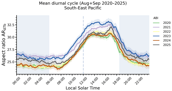
All years show the same temporal patterns, with nearly identical timing of the morning growth onset (around 08:00 LST) and the late-afternoon transition (around 17:00 LST) (Fig. 11). As previously found for λ_LWP, interannual variability primarily affects the amplitude rather than the phase of the cycle. Upscale rates for λ_ΔTb range from 1.08–1.40 km h⁻¹, while downscale rates vary between 2.03 and 2.44 km h⁻¹ (see Table 5). Although slightly larger than in the LWP-derived metric, this dispersion remains small compared to the total diurnal amplitude (of order 10 km), confirming that solar forcing dominates over year-to-year variation.

Here again, a clear contrast emerges between the cell size and the aspect ratio. While λ_ΔTb testifies of a moderate interannual spread in magnitude, this dispersion largely cancels out when considering the normalization by the MBL depth. AR_ΔTb upscale rates vary only between 0.92 and 1.21 h⁻¹ and downscale rates between 1.61 and 1.93 h⁻¹. The diurnal curves from all years almost overlap (Fig. 11b). This mirrors our LWP-based results: interannual variability is primarily expressed in the absolute horizontal scale, whereas the aspect ratio remains tightly constrained over the years.

Finally, as observed in Sect. 4, although ENSO-related changes in sea surface temperature and inversion strength are expected to modulate MBL depth and thus the horizontal scale of organization, the observed year-to-year variability in λ_ΔTb remains difficult to link with a clear, traditional ENSO-phase dependence. However, consistent with our findings for λ_LWP, the cell sizes λ_ΔTb for 2024 stand out as a clear outlier with distinctly lower values. This anomaly aligns with the atypical nature of the 2023–2024 El Niño event discussed previously; the intensified large-scale subsidence and enhanced inversion strength (EIS) effectively compressed the MBL from above, preventing the spatial expansion of cells traditionally expected during warm ENSO phases. Interestingly, this structural distinction becomes minimal when considering the aspect ratio AR_ΔTb consistent with our results for AR_LWP. This suggests that while the structures of the cellular patterns were vertically and horizontally constrained by the enhanced capping inversion, their proportionality remained largely conserved.

Figure 11 Diurnal cycle of (a) λ_ΔTb and (b) AR_ΔTb in SEP region with the ABI/GOES-East accross the years from 2020–2025. Each color represents data for a year. Line is the annual mean from ABI with its standard error envelop.

Table 5 Interannual upscaling and downscaling rates Δ_tλ_ΔTb [km h⁻¹] and Δ_tAR_ΔTb [h⁻¹] derived from ABI observations (August–September, 2020–2025). Upscaling rates are computed between 08:00–14:00 LST and downscaling rates between 17:30–20:00 LST. The last column indicates the interannual mean ± one standard deviation.

6 Sensitivity of spatial metrics to Cloud Fraction

Stratocumulus cellular regimes primarily differ by their cloud fraction (CF) and the relative distribution of cloudy and clear-sky areas (Fig. 3) (Wood and Hartmann, 2006; Wood, 2012; Muhlbauer et al., 2014; McCoy et al., 2017; Mohrmann et al., 2021; McCoy et al., 2023). To capture this variability, we use CF quartiles as a proxy for distinct MBL dynamical regimes, ranging from broken cumulus-like conditions (Q1) to nearly overcast stratocumulus decks (Q4), with intermediate regimes (Q2–Q3) corresponding to transitional states between decoupled and well-mixed boundary layers. The diurnal evolution of these CF quartiles is depicted in Fig. 12, where all four regimes exhibit a progressive decrease in cloud fraction after sunrise followed by a increase in late afternoon. Surprisingly sunrise and sunset times show a local increase in CF, indicating a sensitivity to rapid change in illumination for this cloud property. This evolution is more pronounced for lower CF regimes and remains consistent between ABI and MODIS quartiles.

Figure 12 Diurnal cycle of Cloud Fraction (CF) over the SEP region from ABI/GOES-East, according to CF quartiles. For each quartile, diurnal cycles are averaged over August–September for each year and then over the 2020–2025 period. Lines denote the mean, and shaded envelops the standard error. Shading may be indistinguishable from the lines where the standard error is small. Diamond markers indicate MODIS/Terra and Aqua mean CF and associated standard error for the corresponding MODIS-based quartiles. Uncertainties on diamond markers may not be visible due to marker size.

Both MODIS and ABI LWP-based analyses indicate that the highest CF regime is associated with lower mean cell sizes λ_LWP, and a stronger diurnal growth rates Δ_tλ_LWP (Fig. 13a and Table 6). AR_LWP exhibits likewise a consistent increase in growth rate across CF regimes for both instruments (Table 6). However, the separation in mean AR_LWP across CF quartiles differs between MODIS and ABI, showing opposite tendencies (Fig. 13b). We attribute this discrepancy primarily to differences in the estimation of MBL depth, which is highly sensitive to scene cloud cover, particularly in MODIS retrievals (see Appendix).

For ΔTb, a similar daytime pattern is observed: the mean cell size, λ_ΔTb, decreases, while the diurnal growth rate, Δ_tλ_ΔTb, increases from Q1 to Q4 (Fig. 14a and Table 7). The AR_ΔTb metric further supports these differences in both mean and temporal evolution across cloud regimes, although the separation in daily-averaged values is weaker.

A particularly noteworthy feature concerns the early-morning evolution: around 08:00 LST, all CF regimes display a very similar initial tendency, suggesting a common dynamical response to the rise of Sun (Fig. 14b). However, as the morning growth develops, the four curves progressively diverge. Regimes with larger cloud fraction (Q3–Q4) experience stronger amplification, leading to increasingly separated maxima and more distinct early-afternoon plateaus. This behavior indicates that while the triggering mechanism of mesoscale organization may be shared across regimes, its distinct amplification strongly depends on the cloud fraction state and the MBL regime. The apparent midday plateau, observed in mean diurnal cycles (Figs. 6 and 9), can be reinterpreted here, in light of these CF regimes. It can be understood as a superposition of distinct CF-related behaviors: intermediate regimes (Q2–Q3) undergo a well-defined plateau in early afternoon, whereas this feature is less pronounced in Q1 and tends to disappear in Q4, where a more direct transition from growth to decay is observed. This highlights that the plateau is not a general feature of the diurnal cycle but rather reflects the relative contribution of different cloud regimes and their different dynamics. Low-CF regimes (Q1) show weaker and less coherent diurnal variations, and are more affected by radiative biases at sunrise and sunset, particularly seen with ΔTb derived metrics (Fig. 14). This behavior suggests an enhanced sensitivity of low-CF regimes to the day–night transition, probably linked to more heterogeneous and less stratified cloud fields, to a reduced coupling between cloud organization and the diurnal evolution of the MBL, or to stronger three-dimensional radiative effects at cloud edges (Hogan and Shonk, 2013; Villefranque and Hogan, 2021).

Remarkably enough, the very stable nighttime situation we observed in Figs. 9 and 11 is verified, across CF regimes. Both λ_ΔTb and AR_ΔTb show a steady value for their nocturnal state, with increasing value from Q4–Q1. This result points to the robustness of the nighttime situation: its steadiness is found in any cases, across the year and the cloud organization regimes.

Overall, the shared temporal behavior of all metrics – including those based on LWP and ΔTb – confirms that the mean and interannual daytime evolution and diurnal cycle analyzed earlier are not driven by variations in cloud fraction itself. Instead, CF acts as a modulator of this intrinsic dynamical cycle, primarily controlling its amplitude and intensity. While λ reflects a robust and regime-independent dynamical framework modulated in amplitude by CF, AR provides a more sensitive indicator of regime-dependent morphological adjustments, yet also reveals an underlying compensation mechanism linking mesoscale organization to MBL structure.

These findings raise several important questions regarding the physical mechanisms linking CF, cell growth and MBL structure. For instance, it would be worth investigating why high-CF scenes are systematically associated with smaller cellular structures, why these cells undergo a faster daytime expansion, and to what extend low-CF regimes still experience a morning cell growth despite a reduction in cloud cover through the day.

Figure 13 Diurnal cycle of (a) λ_LWP and (b) AR_LWP over the SEP region from ABI/GOES-East, stratified by CF quartiles. For each quartile, diurnal cycles are averaged over August–September for each year and then over the 2020–2025 period. Lines denote the mean, and shaded areas the standard error. Diamond markers indicate MODIS/Terra and Aqua mean values and associated standard error for the corresponding MODIS-based CF quartiles. Uncertainties on diamond markers may not be visible due to marker size.

Table 6 Upscaling rates Δ_tλ_LWP [km h⁻¹] and Δ_tAR_LWP [h⁻¹] derived from MODIS and ABI observations (August–September, 2020–2025) across CF quartiles. MODIS rates are computed between 10:30–13:30 LST and ABI rates between 08:00–14:00 LST. The last column represents the mean across quartiles.

Figure 14 Same as Fig. 13 but for (a) λ_ΔTb and (b) AR_ΔTb.

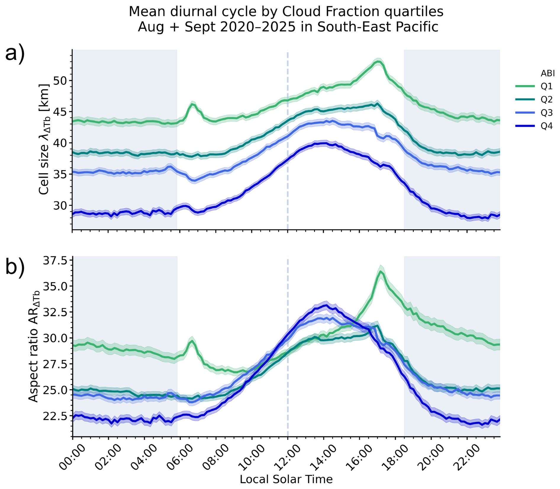
Table 7 Upscaling and downscaling rates (Δ_tλ_ΔTb [km h⁻¹] and Δ_tAR_ΔTb [h⁻¹]) derived from ABI observations (August–September, 2020–2025) across CF quartiles. Upscaling rates are computed between 08:00–14:00 LST and downscaling rates between 17:30–20:00 LST. The last column represents the mean across quartiles.

7 Summarize and Perspectives

Stratocumulus clouds are known to organize into mesoscale cellular convection patterns characterized by varying proportions of cloudy and clear-sky areas. These morphologies have been extensively documented using MODIS observations onboard Terra and Aqua satellites, notably through the derivation of spatial metrics such as cell size λ and aspect ratio AR, obtained from the spectral decomposition of Liquid Water Path (LWP) variance. However, their temporal evolution has remained much less explored. In this study, we extend this framework by addressing, firstly the daytime evolution of λ and AR, with the use of LWP geostationnary observations, secondly its diurnal dynamics with infrared (IR) data. By applying the same spectral decomposition methodology to both LWP and IR geostationary observations, we demonstrate that the brightness temperature difference $\mathrm{\Delta }\text{Tb}={\text{Tb}}_{\mathrm{12.3}\mathrm{\mu }\mathrm{m}}-{\text{Tb}}_{\mathrm{10.3}\mathrm{\mu }\mathrm{m}}$ provides a robust proxy for characterizing mesoscale cellular patterns consistently during both daytime and nighttime. Our work has been focused on the South-East Pacific region, for the two months of August and September 2020–2025, thus providing a robust statistical results.

Our results reveal a pronounced diurnal cycle of stratocumulus mesoscale organization, captured coherently by both LWP- and ΔTb-based diagnostics. An upscale growth phase develops from sunrise reaching a quasi-plateau in early afternoon, that is observed when looking both a the LWP-based daytime evolution and the full ΔTb-based diurnal evolution. This is followed by faster afternoon downscale, while nighttime conditions remain strikingly stable. This temporal structure is invariant across years, and the interannual spread remains small compared to the full diurnal amplitude, demonstrating that solar radiative forcing exerts the primary control on the daily evolution of cloud mesoscale organization.

Beyond this robust diurnal behavior, a central result of this study lies in the contrasted sensitivities of cell size and aspect ratio. While λ exhibits substantial interannual variability in absolute value, AR remains nearly invariant. This contrast holds whether organization is diagnosed from LWP or from ΔTb, confirming that the robustness of AR does not depend on the observational proxy.

A similar distinction emerges across cloud fraction quartiles, which aim to mimic the different low-level cloud regimes, from strongly coupled StCu decks, transitioning to decoupled states, to Cumulus-like regimes. Increasing CF is associated with stronger amplitudes and steeper growth and decay rates of λ, suggesting a tight interdependence between mesoscale organization and the MBL. In contrast, AR displays only minimal differences between CF regimes, with a quasi-overlap of all four diurnal cycles. These results suggest that λ is strongly modulated by MBL variability – which could mirrors both interannual fluctuations and regime dependence – whereas AR reflects a more intrinsic geometric constraint of mesoscale convection.

Altogether, this work highlights the added value of adopting a dynamical perspective on stratocumulus structure. By comparing cell size and aspect ratio, we show that AR provides a unifying metric: it preserves the robust diurnal signal imposed by solar forcing while minimizing interannual and regime-dependent variability linked to MBL. Investigating aspect ratio rather than cell size alone therefore reveals a more intrinsic geometric constraint governing stratocumulus mesoscale organization over the South-East Pacific. Previous studies, notably Wood and Hartmann (2006), reported a robust AR value on the order of 30–40 using Terra observations, with this paper we intend to extend this view by quantifying its full diurnal evolution. We have shown despite substantial variations in years and cloud fraction, AR displays a consistent daytime increase and nighttime recovery.

Understanding the processes controlling the remarkably robust diurnal evolution of AR now emerges as a key scientific challenge. What mechanisms govern this evolution? Is it an emergent property of radiatively driven convection within the MBL? Does it reflect a dynamical balance between horizontal mesoscale circulations and vertical boundary-layer growth? Or is it constrained by larger-scale environmental forcing?

More fundamentally, the persistence of a common AR evolution across years, CF regimes, and throughout the diurnal cycle suggests that stratocumulus mesoscale organization follows a reproducible horizontal-to-vertical scale adjustment. Identifying the processes that govern this behaviour, and understanding how they interact with cloud cover, cellular growth, and MBL structure, remain important open questions for a process-oriented description of stratocumulus dynamics. Another important question is whether this robust AR evolution still hold across the different mesoscale cloud regimes, illustrated in Fig. 3 in the beginning of this paper. In particular, determining if these contrasted structures exhibit similar aspect-ratio dynamics would help reinforce the universality of the dynamical framework proposed here.

Addressing these questions requires moving beyond the Eulerian framework used here. Future work will investigate the diurnal evolution over consecutive days in a Lagrangian perspective (Eastman and Wood, 2016; Eastman et al., 2016, 2022; Smalley et al., 2022; Lewis et al., 2023; Lewis and Bellon, 2025), tracking air masses to assess whether the observed AR invariance is locally set by daily radiative forcing or controlled by the history and origin of the boundary-layer air masses. Such an approach would help determine whether the geometric constraint is dynamically maintained along trajectories or periodically reset by large-scale forcing through several days.

Further exploration of the energetic budget, for instance with the use of Large Eddy Simulations, would allow us to better identify the mechanisms that govern this geometric constraint – particularly mesoscale circulations and entrainment processes within the MBL that likely monitor the horizontal-to-vertical scale coupling (McMichael et al., 2019; Zhou and Bretherton, 2019; Brient et al., 2024).

Finally, extending this analysis to other stratocumulus regions will allow to test the universality of this AR invariance. If similar geometric stability is observed over the North-East Pacific (using GOES-West geostationnary satellite), Namibia (MSG and MTG satellites), or West Australia (Himawari satellite) despite differences in aerosol loading, continental influence, or synoptic forcing, it would strongly support the hypothesis that AR represents a fundamental dynamical attractor of stratocumulus mesoscale organization.

Appendix A: MBL estimation and discrepancies between MODIS and ABI

We first applied the same methodology to estimate the marine boundary layer (MBL) depth from both MODIS and ABI datasets. However, the resulting diurnal cycles of MBL depth as a function of cloud fraction (CF) quartiles (Fig. A1a) reveal substantial inconsistencies between the two instruments when using a cloud top height (CTH)-based approach.

Fragmented cloud scenes (Quartile 1) are generally associated with a deeper MBL, while overcast conditions (Quartile 4) correspond to a shallower MBL (Wood, 2012). This expected behavior is captured by ABI but not reproduced in the MODIS-derived estimates.

This discrepancy seems to arise from limitations in the MODIS retrievals. Due to its higher sensitivity, MODIS tends to produce artificial low cloud top temperature (CTT) and cloud top height (CTH) values in prevalence of thin clouds and at cloud edges Eastman et al. (2016). As a result, the simple method directly based on CTH lead to a systematic underestimation of MBL depth in MODIS data, thereby yielding physically inconsistent diurnal variations, in particular for low-CF regime (Quartile 1).

This highlights the need to account for cloud fraction when deriving a representative MBL depth at the scene scale. To address this issue, we adopt the method of Eastman et al. (2016), in which a representative CTT is determined using an adaptive threshold based on the mean CF. Looking at a cloud scene, a 5 K bins histogram of CTT is firstly computed. Then, the authors assume that in overcast conditions, the largest peak in CTT histograms represents the temperature at the top of the MBL. However, in more broken cloud scenes, they postulate the top of the MBL is colder than the most populous CTT bin in the histogram, owing to the increased prevalence of thin clouds and cloud edges in the sample. Therefore, for cloud scenes with less than overcast cloud cover (under 90 %) they “tune” the histogram sampling by decreasing the sampling threshold on the cold side of the peak along with the smaller cloud fraction. The threshold value is decided in order to match the active Lidar CALIPSO data. Values and illustrated examples of thresholds are given in Eastman et al. (2016) Fig. 2 and Table 1. Finally, the corresponding CTH (and thus MBL depth) is then inferred from this adapted CTT, the sea surface temperature (SST), and the Lapse rate (Γ) parameterization of Wood and Bretherton (2004) and Zuidema et al. (2009).

$$\begin{array}{}\text{(A1)}& \text{CTH}={\displaystyle \frac{\text{SST}-\text{CTT}}{\mathrm{\Gamma }}}.\end{array}$$

This approach improves the consistency between datasets. In particular, it reduces the underestimation of MODIS-derived MBL depth relative to ABI and restores a quite physically consistent dependence of MBL depth on CF quartiles (Fig. A1b). We therefore retain this method for MBL estimation from MODIS.

Figure A1 Diurnal cycle of MBL depth in SEP region with the ABI/GOES-East dataset, according to CF quartiles. Values computed with the same method as ABI (a) and with method from Eastman et al. (2016) (b). The color matching diamond markers represent the mean and standard error obtained with MODIS/Terra and Aqua for the MODIS-based CF quartiles.