Synthesis of surface snowfall rates and radar-observed storm structures in 10+ years of northeastern US winter storms

Winter storms can cause disruptions in the densely populated regions of the northeastern United States. Mesoscale snow bands embedded within winter storms are often the main focus of snowfall forecasts and analyses. While primary bands are associated with frontogenesis, multi-bands are found in environments with both frontogenesis and frontolysis. This study investigates the relationship between observed surface snowfall rates and local enhancements in radar reflectivity (i.e., mesoscale snow bands) using data from 264 storm days over 11 winter seasons (2012–2023). We compare hourly surface snowfall rates obtained by National Weather Service (NWS) Automated Surface Observing Systems (ASOS) weather stations with the area × time fractions of locally enhanced reflectivity features and of all echoes passing over the 25 km radius of the surface observation. Our analysis focuses on non-orographic snowstorms with surface winds < 5 m s⁻¹.

Our findings show that most of the time snow rates are low (75 % of hours had liquid-equivalent snow rates less than 1 mm h⁻¹). Heavy snow rates (>2.5 mm h⁻¹ liquid equivalent) are rare (<4 % of observations). When enhanced reflectivity features pass over a location, only 1 out of 4 h have heavy surface snow rates. High-spatial-resolution vertical cross-sections from airborne radar obtained during the NASA Microphysics and Precipitation for Atlantic Coast-Threatening Snowstorms (IMPACTS) field campaign and rapid-update range-height indicators (RHIs) from ground-based radar demonstrate that enhanced reflectivity features in snow aloft are tilted and smeared on their way to the surface as their constituent snow particles are dispersed laterally by the horizontal winds within the storm. The duration of all snow echo over a location is useful in determining where higher snowfall accumulations may occur.

1 Introduction

The intersection of high population density and winter weather in the northeastern United States yields more frequent disruptive societal impacts compared to winter weather in other US regions (Kocin and Uccellini, 2004; Novak et al., 2023; Guarino and Firestine, 2010). This geographic region encompasses the states of Pennsylvania, New Jersey, New York, Connecticut, Rhode Island, Massachusetts, Vermont, New Hampshire, and Maine and includes the urban corridor spanning the cities of Philadelphia, New York, and Boston. The geography includes portions of the Appalachian Highlands and Atlantic Coastal Plain (Fenneman, 1928). In general, storms in the region have negligible to weak orographic forcing, except a few areas with higher peaks.

US National Weather Service (NWS) forecasters use a variety of methods to predict snowfall accumulations. From numerical models, they use ice water context (IWC) as well as the presence of banded features in simulated reflectivity to estimate quantitative precipitation (Radford et al., 2023). For nowcasting, NWS forecasts use observed radar reflectivity to determine locations of heavy snow (David Novak, personal communication).

Much previous work on diagnosing heavy snow rates in northeastern US winter storms has focused on mesoscale snow bands, elongated features of enhanced radar reflectivity observed by operational scanning radars. Snow bands that are longer than 200 km are called primary bands and are associated with strong frontogenesis at low levels and mid-levels in the storm (Novak et al., 2004, 2010; Ganetis et al., 2018; Kenyon et al., 2020; Baxter and Schumacher, 2017). Bands that are shorter than 200 km and typically occur in groups are known as multi-bands. Previous work related to winter storms in the northeastern US has often focused on primary bands and understanding their associated physical mechanisms (e.g., Novak et al., 2004, 2008, 2009, 2010; Novak and Colle, 2012; Kenyon et al., 2020; Stark et al., 2013). The relationship between multi-bands and frontogenesis is not clear as multi-bands are found in a wide range of frontogenesis environments including negative values (frontolysis) (Ganetis et al., 2018; Nicosia and Grumm, 1999; Connelly and Colle, 2019). Han et al. (2007) examined the precipitation structure of two winter storms and found that couplets of frontogenesis and frontolysis were present in the vicinity of both the occluded front and the warm front. The physical mechanisms and relative importance of different types of instabilities (potential, conditional, shear, conditional symmetric) to multi-band production is a topic of active research (e.g., Shields et al., 1991; Ganetis et al., 2018; Leonardo and Colle, 2024; Varcie et al., 2022; Zaremba et al., 2024).

Case studies of northeast winter storms have usually focused on extreme events with high snowfall accumulations and strong frontogenesis (e.g., Picca et al., 2014; Varcie et al., 2022; Ganetis and Colle, 2015; Novak et al., 2008; Han et al., 2007; Colle et al., 2014; Clark et al., 2002; Lackmann and Thompson, 2019). But the relative prominence of different physical processes in an extreme event may not be analogous to that for a more typical, weaker winter storm. The practice of generalizing extreme events as representative of typical events implies that extreme events are a clearer, more “pure” representation of the key physical processes rather than a low-probability juxtaposition of circumstances that amplify snowfall. The assumption of representativeness of extreme events for more typical winter storms needs to be evaluated with evidence from a large sample size.

While most of the snow band literature has focused on the northeastern US, non-orographic snow bands have been documented in winter storms across the world. Lake/sea-effect snow banding has been investigated in Europe and Japan (Mazon et al., 2015; Norris et al., 2013; Fujiyoshi et al., 1998; Murakami, 2019; Sato et al., 2022). Winter storms in eastern Asia (China, Russia, Korea) also exhibit banded features (Zhao et al., 2020).

We use NWS Next-Generation Radar (NEXRAD) and National Weather Service (NWS) Automated Surface Observing Systems (ASOS) data from 264 snowstorm days in the northeastern US to determine if the relationships illustrated in outlier case studies between radar-observed snow bands and heavy surface snowfall withstand scrutiny with a large dataset. We also examine recent field campaign observations of the detailed vertical structures within winter storms from airborne radars deployed during the recent NASA Investigation of Microphysics and Precipitation for Atlantic Coast-Threatening Snowstorms (IMPACTS) field campaign (McMurdie et al., 2022) and from ground-based radars at Stony Brook University (KASPR; Oue et al., 2017).

There are several complicating factors in the analysis of winter storms using weather radar observations. Increases in radar reflectivity in snow do not necessarily equate to increases in mass per unit volume (Table 1). Aggregation and partial melting increase the radar reflectivity but do not change the mass per unit volume. Additionally, there are important differences between the 3D structures of enhanced reflectivities in rain versus snow. In warm-season precipitation systems the 0 °C level is 3 km altitude or more above the surface, and it is reasonable to deduce that stronger locally enhanced radar reflectivity features a few kilometers above the surface are associated with higher rain rates at the surface. The typical fall speeds of raindrops (∼2–8 m s⁻¹, depending on raindrop size) often yield nearly vertical columns of enhanced reflectivity features in rain layers. In contrast, the slower fall speed of snow (∼1 m s⁻¹, equivalent to 33 min to fall 2 km) yields sufficient time for the advection of the snow by horizontal winds, which are typically ≥10 m s⁻¹, to form curved ice streamers (Wexler, 1955; Wexler and Atlas, 1959). Falling snow particles can be blown sideways more than 50 km horizontally from the locations where they first achieve precipitation size near the top of the storm.

Table 1 Table of microphysical processes and their associated change to mass per unit volume (IWC and LWC), as well as radar reflectivity. Radar reflectivity is a function of diameter and dielectric constant. The dielectric constant is larger for liquid water than for ice particles. Italics are used for emphasis.

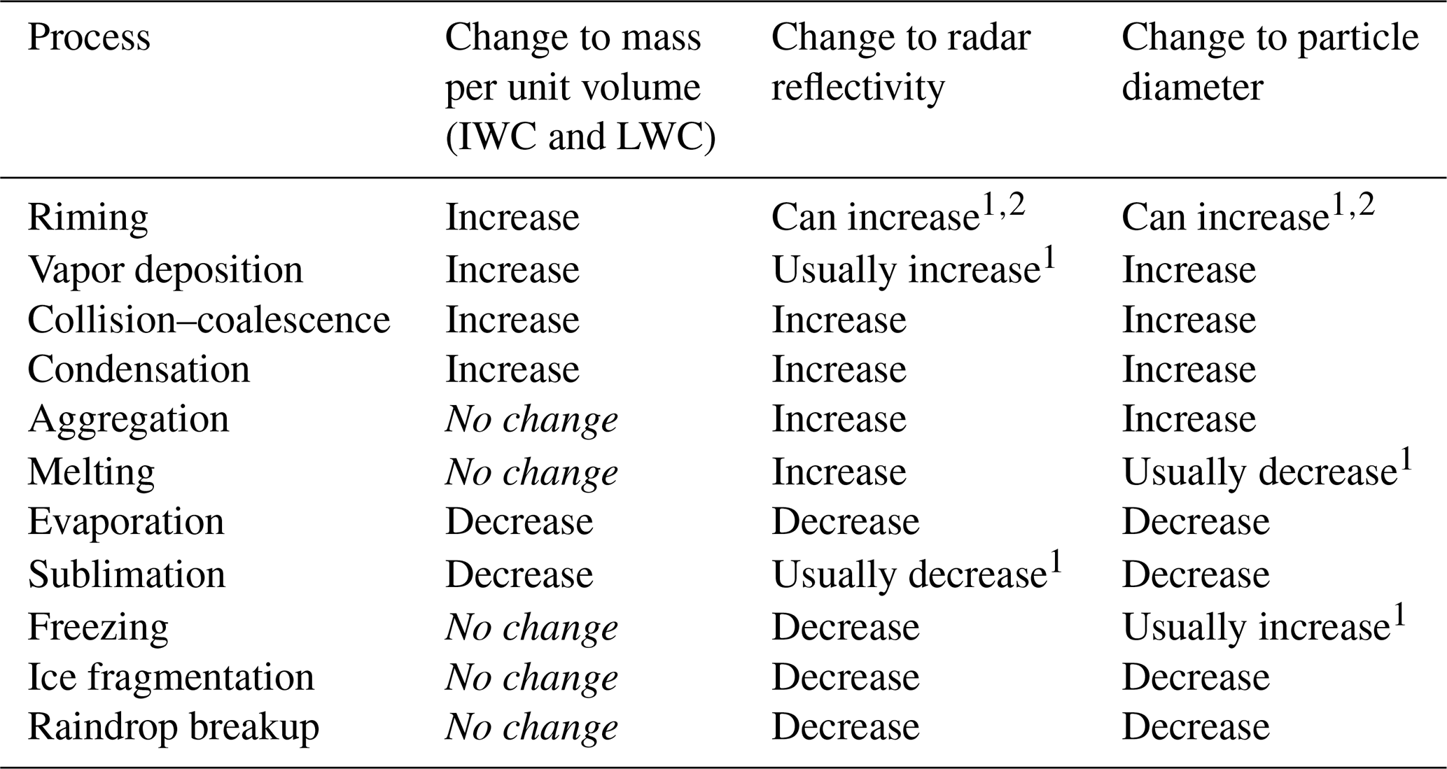
¹ Depends on ice crystal shapes and densities of preexisting precipitation particles. ² Depends on the degree of riming. For example, light riming will not change reflectivity or diameter much if at all.

Further, there is a large variation between observed ice water content (IWC) and reflectivity in ice clouds and light snow (Zaremba et al., 2023). Coincident observations of IWC and radar reflectivity collected during research aircraft flights as part of the Seeded and Natural Orographic Wintertime Clouds: the Idaho Experiment (SNOWIE) field campaign in the mountains of Idaho (Tessendorf et al., 2019) illustrate the joint frequency distribution of this relationship (Fig. 1). These IWC and Z data for surface-snow-producing clouds over the mountains of Idaho do not include any partially melted particles but may include aggregates. For reflectivities > 0 dBZ, which usually contain some precipitation-sized falling ice particles, IWC generally increases as Z increases. But given the spread of the observed values, there is at least a factor of 2 uncertainty in the volumetric ice mass as a function of radar reflectivity (Fig. 1; Zaremba et al., 2023).

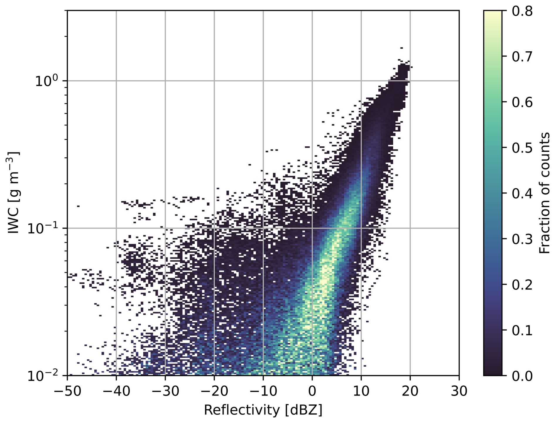
Figure 1 Joint distribution based on over 100 000 coincident aircraft observations of 1 Hz Nevzorov probe ice water content samples and Wyoming Cloud Radar reflectivities obtained in light snow by the University of Wyoming King Air during the SNOWIE project in the mountains of western Idaho. Reflectivity values at the aircraft flight level were calculated by linear interpolation between the first valid range gates above and below the aircraft. Adapted from Fig. 6 in Zaremba et al. (2023).

The overarching goal of this study is to explore and understand the relationships between surface snow rates and locally enhanced reflectivity features (i.e., snow bands) in winter storms. The key finding is that locally enhanced linear features (i.e., mesoscale snow bands) in operational scanning radar reflectivity within northeastern US snowstorms (which exclude orographic and lake-effect snowstorms) are usually not associated with heavy hourly liquid-equivalent surface snow rates.

2 Data and methods

2.1 10+-year winter storm dataset

We use observations from 264 storm days in the northeastern US from over 10 years (2012–2023) to ensure we are studying the relationships over a large representative sample. Following the methodologies of Hoban (2016) and Ganetis et al. (2018), we define a winter storm as any date within the months of October to March for the years 2012–2023 where at least 25.4 mm (1 inch) of snow depth was reported over a 24 h period for at least two out of 14 stations shown in Fig. 2b. We used a threshold of 25.4 mm to include a wide range of storms in our analysis and not only those that produce a large snow accumulation. The daily snow depth data at each station were gathered from the Global Historical Climatology Network daily (GHCNd) database (Menne et al., 2012). We selected the subset of 14 stations to focus on storms that impacted the more densely populated regions of the northeastern US and to minimize the inclusion of storms that were predominantly lake-effect snow events. While the majority of the stations we use to define winter storm events are close to the coast, it is possible by using the Albany, NY, and Binghamton, NY, stations that some lake-effect events are included in our dataset. Lake-effect snow bands passing overhead have a documented relationship to heavier snow rates (Kristovich et al., 2017; Kosiba et al., 2019; Mulholland et al., 2017) so their inclusion in the dataset could slightly bias the results toward a stronger relationship between snow bands and heavier surface snow than is true for stations further from the Great Lake shores.

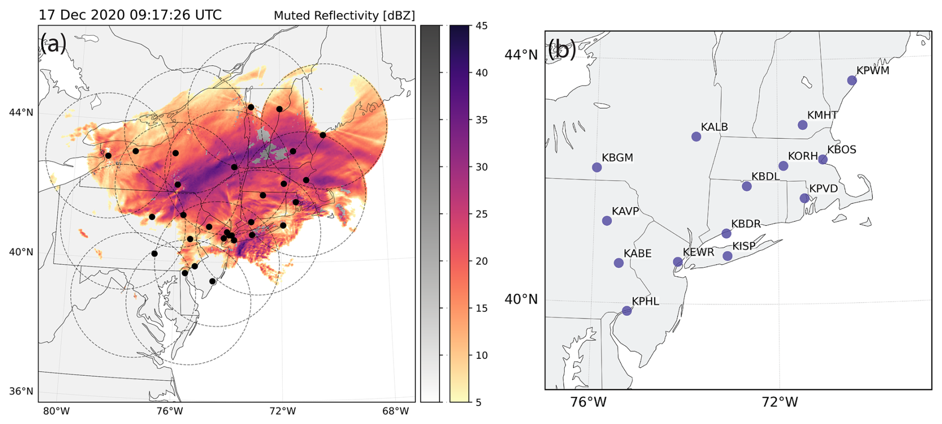
Figure 2 (a) An example of the reflectivity mosaic from 27 December 2020 at 09:17 UTC. Black dashed circles indicate the 200 km extent from each radar used in the mosaics. Black dots indicate ASOS stations where the hourly snow rate is used in the analysis. (b) Map of ASOS stations where daily snowfall accumulation is used to define a winter storm in this analysis.

The years 2012–2023 were chosen since 2012 is the start of the period when dual-polarization radar data are available from US NWS radars. Use of dual-polarization products allows us to remove melting and mixed precipitation observations, often confused for heavy snow, from our analysis (discussed in Sect. 2.1.3). The full list of storms is tabulated in Table S1 in the Supplement.

2.1.1 Hourly surface station observations

Hourly observations from 29 ASOS stations in the northeastern US are used to quantify the liquid-equivalent snowfall rates during each winter storm day (Fig. 2). The hourly snowfall rates represent hourly liquid-equivalent accumulation and are not instantaneous snow rates. ASOS data are obtained from the online MADIS database (https://madis-data.ncep.noaa.gov/index.shtml, last access: 1 September 2024). Measuring snow with precipitation gauges can be challenging as snow is easily blown sideways by the wind and does not always make it into the gauge (Bruce and Clark, 1966; Groisman and Legates, 1994; Rasmussen et al., 2012; Kochendorfer et al., 2022). To ensure we are getting the best measurements, we only use ASOS stations equipped with all-weather precipitation accumulation gauges (AWPAGs) as these gauges are more skilled at measuring liquid-equivalent snow accumulation than other types of gauges (Martinaitis et al., 2015). The AWPAG sensors are equipped with Tretyakov or double Alter-style shields, which are more accurate at measuring frozen precipitation than gauges with no shields (Rasmussen et al., 2012). AWPAG sensors do not have a heated rim and are thus subject to capping, although it is difficult to estimate how often this occurs in our dataset (Martinaitis et al., 2015). If capping does occur, no snow would be reported for 1 h, resulting in an underestimation of the snow accumulation for that hour. Partial capping can also occur and would result in an underestimation of snow for a period of time followed by an overestimate once the cap releases (Baker Perry, personal communication). To further ensure that we are using reliable observations, only quality-controlled observations when the wind speed is <5 m s⁻¹ are used in our analysis (Rasmussen et al., 2012). The collection efficiency of frozen precipitation is 1.0 at a wind speed of 0 m s⁻¹ and drops to 0.25 at a wind speed of 6 m s⁻¹ for double Alter-shielded gauges, which is why we chose a threshold of 5 m s⁻¹ (Rasmussen et al., 2012). The wind speed threshold removes ∼45 % of hourly snow observations. The distribution of removed measurements is relatively uniform over the entire range of precipitation rate observations (see Fig. 2.6 in Tomkins, 2024a). Observations are only used in the analysis if the station has reported snow for at least 4 h to ensure we are using observations from consistent snow observations and not any short-lived, low-impact events.

Following the guidelines of the Society of Automotive Engineers International Ground Deicing Committee and NCAR, we use a liquid-equivalent precipitation rate threshold of 2.5 mm h⁻¹ to distinguish heavy snow from light (<1 mm h⁻¹) and moderate (1–2.5 mm h⁻¹) snow (Rasmussen et al., 2001). We will use the term heavy to describe snow rates > 2.5 mm h⁻¹ liquid equivalent.

An example time series of liquid-equivalent precipitation rates from Boston, MA, on 7 February 2021 is shown in Fig. 3. Hourly observations that are used in the analysis are represented by a blue bar spanning the hour that the precipitation accumulates. Trace values (0 mm h⁻¹) are considered in the analysis (17:00 UTC), while observations when no precipitation fell are not (06:00–16:00 UTC). The example also shows observations not used in the analysis where the wind speed threshold is exceeded (22:00–00:00 UTC) (plus sign in Fig. 3).

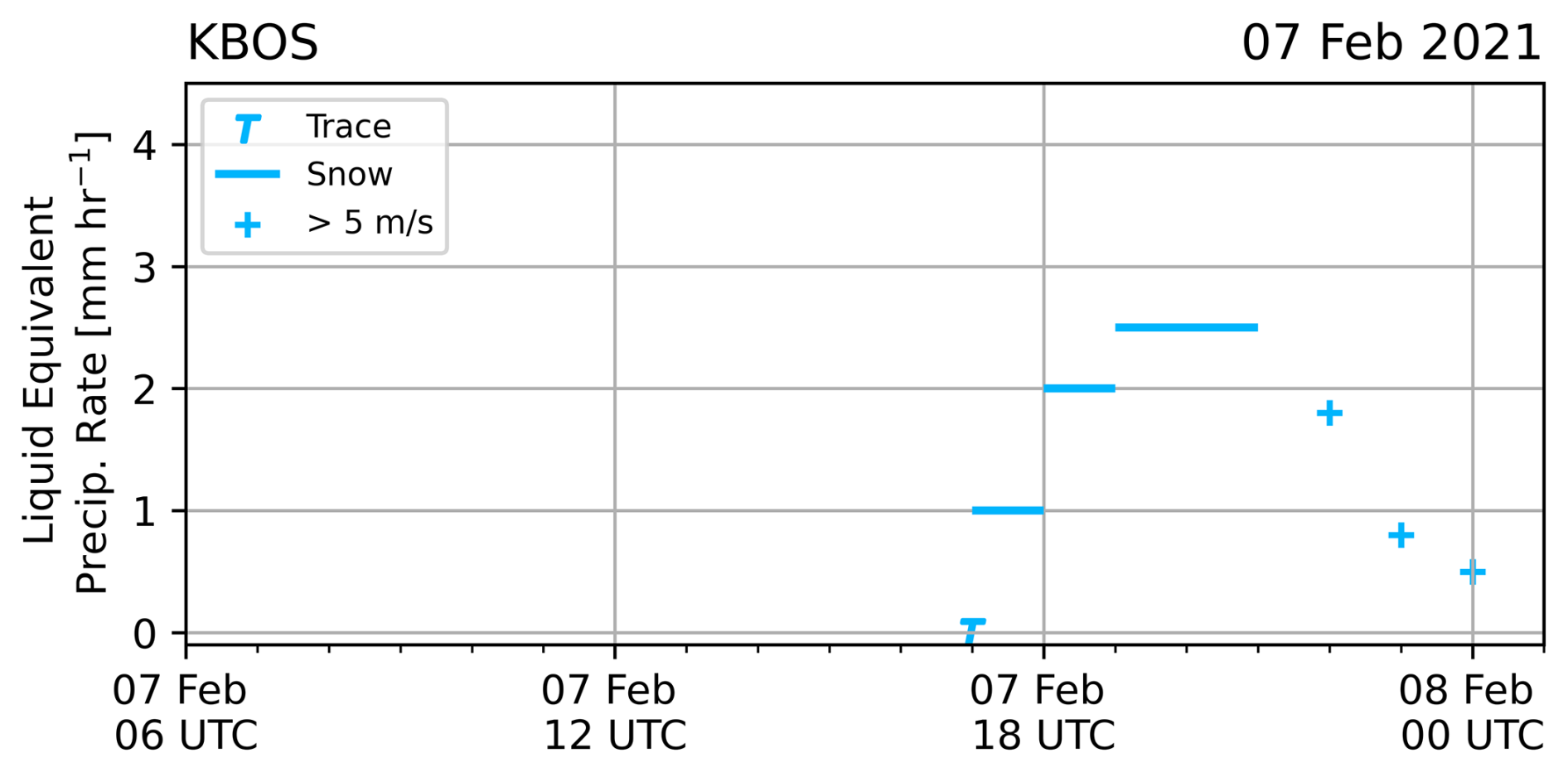
Figure 3 Example time series of the liquid-equivalent precipitation rate [mm h⁻¹] from the Boston, MA, ASOS station (KBOS) from 7 February at 06:00 UTC to 8 February 2021 at 01:00 UTC. Precipitation rates are represented as a bar spanning the hour they were accumulated. Plus signs indicate times when the wind speed is >5 m s⁻¹, and T indicates times when trace amounts of precipitation where observed.

2.1.2 Regional radar mosaics

We use radar observations from the NWS NEXRAD network in the northeastern US to analyze features of the radar reflectivity field in winter storms. All NEXRAD data were obtained from the NOAA archive on Amazon Web Services (Ansari et al., 2018). The NEXRAD instruments scan 360° in azimuth over sets of elevation angles that vary with the selected volume coverage pattern. In this analysis we use the elevation angle at 0.5° above the horizon as 0.5° is the lowest angle common to the different volume coverage patterns. We interpolate the single elevation to yield a 2D grid using Cressman weighting (Cressman, 1959, for full details see Tomkins et al., 2022). We found that interpolation among elevation angles, as is done in the NWS 3D interpolated radar reflectivity product (Smith et al., 2016), often smoothed out gradients bounding locally enhanced reflectivity features of interest.

Our radar data processing utilizes the open-source Python Atmospheric Radiation Measurement (ARM) Radar Toolkit (Py-ART) developed by the Department of Energy ARM Climate Research Facility (Helmus and Collis, 2016). We combine data from multiple radars in the northeastern US into a mosaic on a Cartesian grid over an area of 1202 km × 1202 km with 2 km horizontal grid spacing. The radars used to create the mosaics and an example mosaic are shown in Fig. 2. Regional mosaics are generated for 5–10 min time steps during each storm. Tomkins et al. (2022) detail the quality control, interpolation, and other data processing steps to produce the mosaics.

2.1.3 Objective detection of snow bands

Identifying and locating regions of locally enhanced reflectivity can often be subjective and inconsistent from observer to observer. To mitigate this, we developed a technique that objectively identifies local enhancements in radar observations (Tomkins et al., 2024a). Previous methods to detect enhancements in enhanced reflectivity features in the rain layers of storms, such as convective precipitation cells, did not work well for detecting snow bands. Locally enhanced reflectivity features in snow have more diffuse edges and smaller relative differences compared to the background values than convective cells in rain layers. The technique we employ uses two adaptive thresholds to identify objects based on their distinctness (faint or strong) from the background average. We identify objects in a snow rate field that has been rescaled from reflectivity in order to define local enhancements based on spatial gradients that are roughly linear in snow rate. To rescale the reflectivity, we use the wet snow Z–S relationship from Rasmussen et al. (2003): Z_e=57.3S^1.67, where Z_e is equivalent radar reflectivity with units of mm⁶ m⁻³ and S is liquid-equivalent snow rate with units of mm h⁻¹. Note that the snow rate obtained from this relationship represents an instantaneous liquid-equivalent snow rate from a single radar scan and is hence not expected to match the hourly accumulation liquid-equivalent reported from the ASOS stations. The algorithm outputs a feature detection field which classifies each grid point with radar echo as either part of a “faint feature”, a “strong feature”, or “background”. Details on the feature detection algorithm including multiple examples of reflectivity fields, snow rate fields, and the identified features are provided in Tomkins et al. (2024a). Example reflectivity, snow rate, and feature classification fields are shown in Fig. 4.

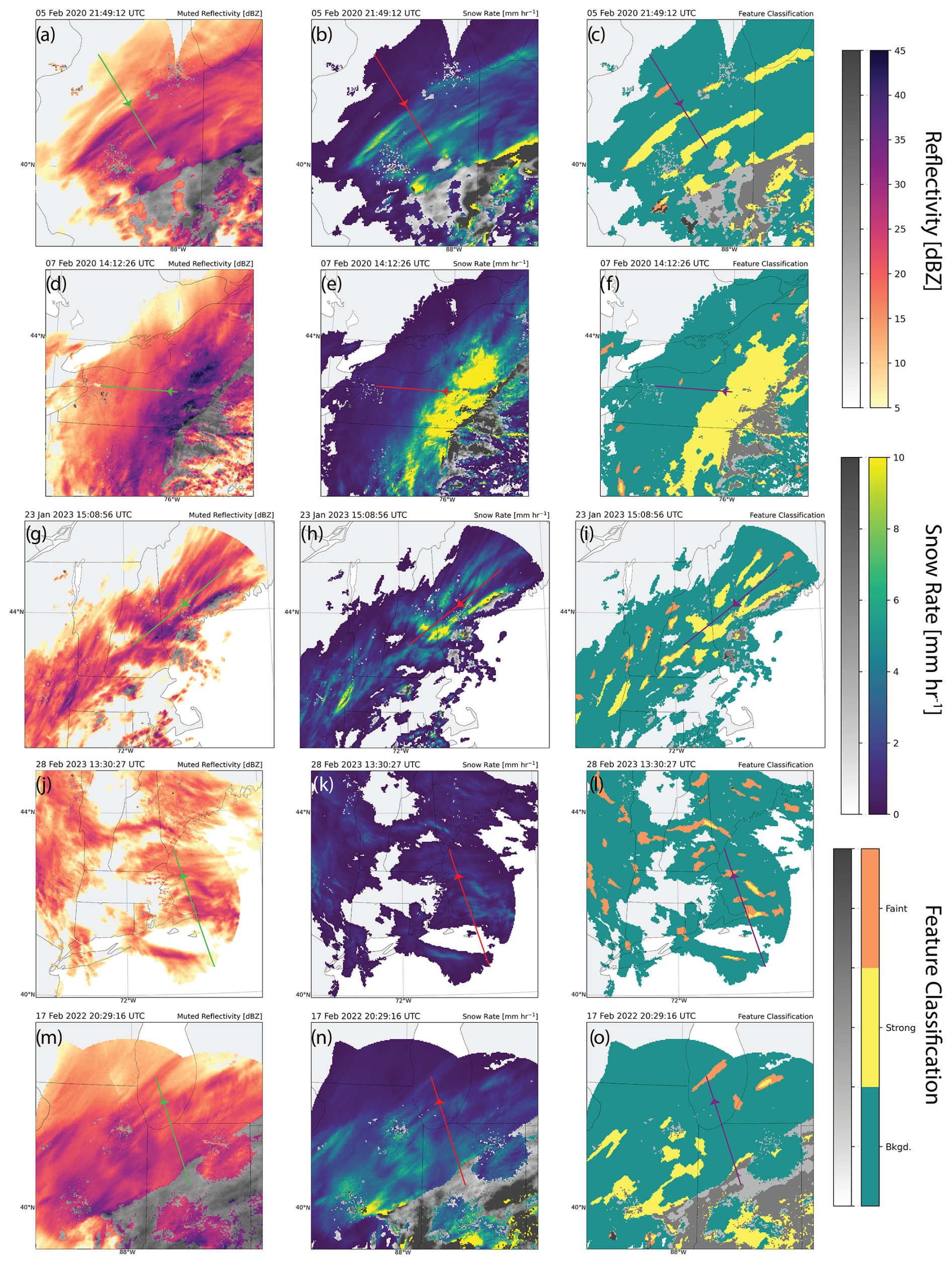
Figure 4 Locally enhanced reflectivity feature classification for the examples presented in Sect. 3.2.2 (Figs. 13–17). Each row shows a different example. (a–c) 5 February 2020 at 21:49:12 UTC, (d–f) 7 February 2020 at 14:12:26 UTC, (g–i) 23 January 2023 at 15:08:56 UTC, (j–l) 28 February 2023 at 13:30:27 UTC, (m–o) 17 February 2022 at 20:29:16 UTC. The left column shows step 1, the input radar reflectivity (dBZ). The middle column shows step 2, the reflectivity field rescaled to the estimated liquid-equivalent snow rate [mm h⁻¹]. Panels (c), (f), (i), (j), and (o) show step 3, the feature classification into faint and strong local features and background values. Each field is image-muted to reduce the visual prominence of melting and mixed precipitation (grayscale) following Tomkins et al. (2022). Green, red, and purple lines indicate NASA ER-2 flight paths, and arrowheads indicate the location of the aircraft at the time of each plot. The feature classification method is detailed in Tomkins et al. (2024a).

The relationship between reflectivity and liquid-equivalent snow rate has large uncertainty as it depends on the ice particle shape, density, degree of riming, aggregation, and terminal velocities of the snow particles present. It would not be suitable to use the quantitative values from a single Z–S relationship (e.g., Fujiyoshi et al., 1990; Mitchell et al., 1990; Rasmussen et al., 2003; Matrosov et al., 2008; von Lerber et al., 2017; Wen et al., 2017). We developed our technique based on the method of Krajewski et al. (1992), who used an area–threshold method to estimate mean areal rainfall using radar reflectivity observations. Krajewski et al. (1992) found that when there is high uncertainty in the Z–R relationship, the rainfall estimates from the area–threshold method perform significantly better than the estimates from the Z–R relationship. Our area × time fraction method estimates space–time integrals from quantities derived from radar reflectivity spatial patterns, thereby avoiding issues that would result from using a highly uncertain transformation from reflectivity to snow rate. Yeh and Colle (2025) compared several different identification methods for identifying snow bands in winter storms and found that object-based methods performed better than methods using absolute or variable reflectivity thresholds.

Transitions between snow, rain, and partially melted snow are common in northeastern US winter storms, which complicates the interpretation of reflectivity since melting and mixed precipitation have higher reflectivities than volumes of only ice or only liquid particles of the same mass. We identify regions of mixed or melting precipitation by combining information from the radar reflectivity and correlation coefficient dual-polarization fields (Tomkins et al., 2022). We remove regions identified as mixed and melting precipitation from our analysis and reduce the visual prominence of these regions in our visualizations using “image muting” (Tomkins et al., 2022). The image-muted regions are depicted in grayscale in regional maps shown as part of subsequent figures.

2.2 Area × time fraction

A main goal of this project is to understand the impact of locally enhanced reflectivity features on the hourly surface snow rates. To accomplish this, we focus on the echo classified as features (from the methods discussed in Sect. 2.1.3) within 25 km of the ASOS station. The regional radar mosaics occur every 5–10 min, so in order to distill the echo area over the hour, we computed an integrated metric called the area × time fraction. Figure 5 illustrates the echo area data that go into calculating the area × time fraction. We separately examine the feature area × time fraction calculated for the echo classified as features (both strong and faint) and the all-echo area × time fraction (strong and faint features plus background echo).

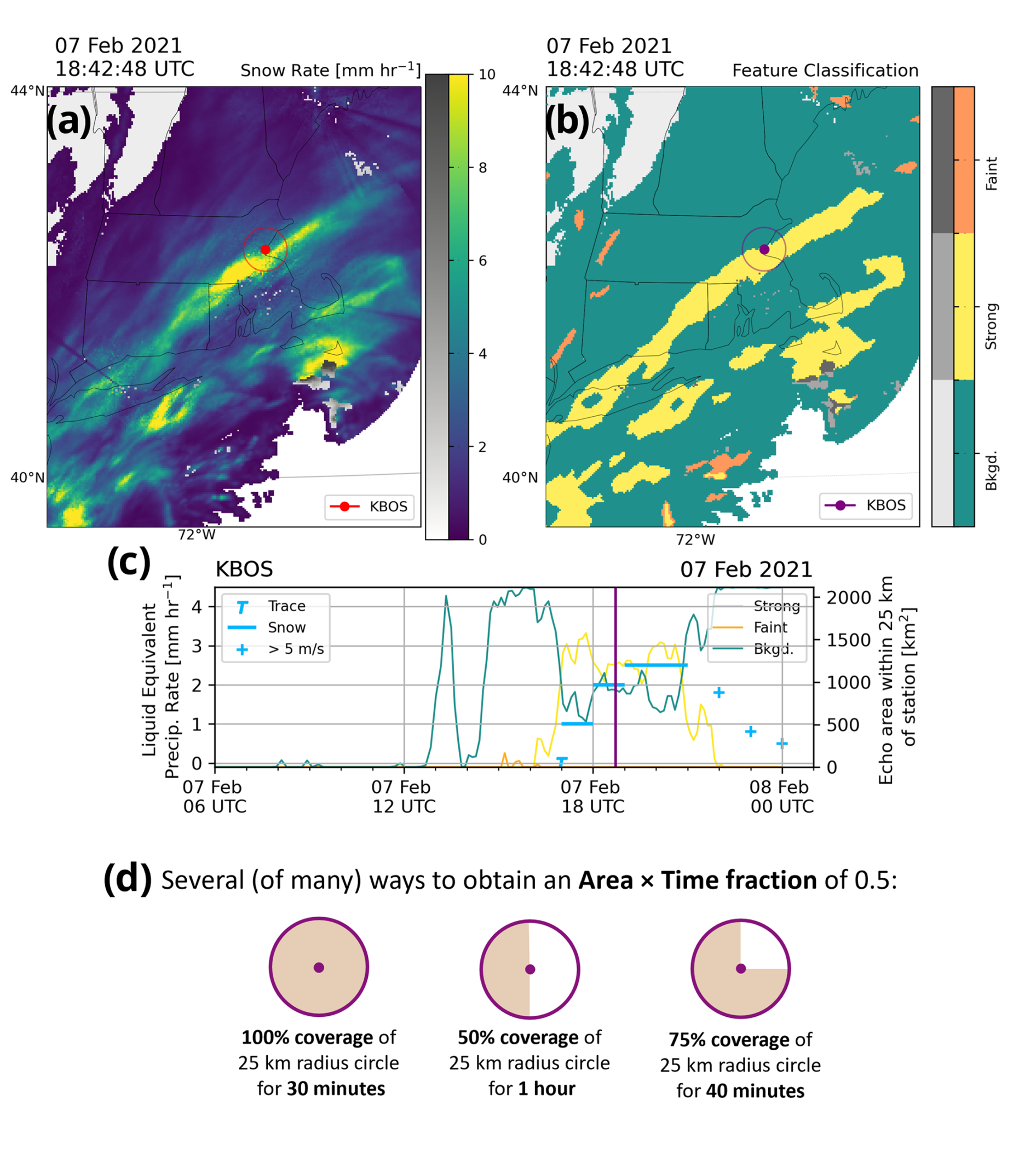
Figure 5 Illustration of how areal radar data and point measurements of snowfall rates are combined. Panel (a) shows the liquid-equivalent snow rate field and (b) shows the feature detection field centered on Massachusetts for 7 February 2021 at 18:42 UTC. (c) The corresponding time series of ASOS hourly precipitation rate (left axis) valid from 7 February at 06:00 UTC to 8 February 2021 at 01:00 UTC and echo areas (right axis) calculated within 25 km of the Boston, MA, ASOS station – KBOS: red dot in (a) and purple dot in (b). Lines in time series (c) correspond to background echo area (teal), strong area (yellow), and faint area (orange) within 25 km of the KBOS station (rings in a and b). The purple vertical line annotated on time series (c) indicates the time of the maps. (d) Several examples of echo coverage over a given time that would yield an area × time fraction of 0.5.

To calculate the area × time fraction we sum the area surrounding the station within a 25 km radius for that hour and then we divide by the total seconds in 1 h and the total area surrounding the station within 25 km, which yields a unitless fraction. Figure 5d demonstrates three scenarios (of many) that would yield an area × time fraction of 0.5. A feature area × time fraction of 1 would indicate the entire surrounding region is filled with feature echo for the entire hour, and a fraction of 0 would indicate no feature echo in the surrounding region for the entire hour.

2.3 Low-pressure center tracks

For each winter storm, we computed the low-pressure center storm track from the ERA5 hourly reanalysis mean sea level pressure (Hersbach et al., 2020) using the methods of Crawford et al. (2021). We subset the global 0.25° resolution ERA5 mean sea level pressure (MSLP) field to the region of eastern North America (−90 to −60° E, 2  to 55° N). For a given winter storm day, we track over ±1 d to capture the full evolution of a given low-pressure system. To find a single minimum for a given time, we first find all the local minima in the MSLP field using a 200 km search radius. Unlike Crawford et al. (2021), we use the ERA5 data in native coordinates, so the grid size in kilometers varies slightly between grid boxes. To avoid finding pressure minima that skip along edges of our defined eastern North America region, we only consider minima where at least 75 % the 200 km search radius is within the region. Following Crawford et al. (2021), minima found from the MSLP field are only considered if they have a pressure gradient of at least 7.5 hPa per 1000 km. We compared the low-pressure center minimum to the set of pressures at a 200 km range from the low-pressure center. To meet the threshold criteria, the mean difference between minimum pressure and the set of pressures at the 200 km range must be at least 1.5 hPa. Once all the local minima have been found for the entire period, we then loop through the period again to select a single minimum for each time since there may be no minimum, one minimum, or multiple minima for each time. In the case of multiple minima we choose the minimum that meets most of the following: minimum which is closest geographically to the previous minimum, minimum with the strongest pressure gradient, and the minimum with the lowest MSLP value. If the closest, strongest, and deepest minima are all different points, we choose the closest minima. If the next point is more than 200 km away from the previous point, we consider this a new system and new track. We filter the tracks to remove tracks that travel less than 250 km or exist for less than 6 h. Finally, we remove any points on the tracks where the MSLP is greater than 1010 hPa.

All tracks between 2012 and 2023 that meet our winter storm criteria defined in Sect. 2.1 are shown in Fig. 6. The density of tracks shows a clear tendency for low-pressure centers to be near the coastline or over the ocean and to move southwest to northeast roughly parallel to the coast (Fig. 6). This pattern is consistent with climatological studies of cyclone tracks (e.g., Bentley et al., 2019). There is a lack of low-pressure locations along/to the east of the Appalachian Mountains, which we suspect is due to our criteria for defining a snowstorm for this study (Sect. 2.1). Since we are only looking at events where stations along the coast and slightly inland in the northeastern US produce snow, tracks along the Appalachian corridor may not produce enough snow within our region of interest to be considered in our dataset.

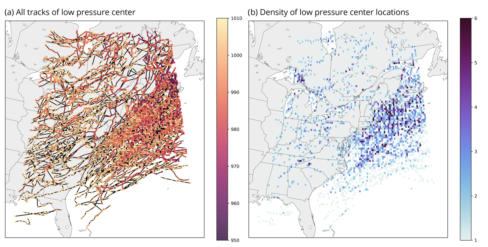
Figure 6 Map of (a) all tracks of low-pressure centers and (b) density of low-pressure center locations for events between 2012–2023 for the region shown. Color shading indicates low-pressure magnitude in hPa units.

Hourly liquid-equivalent snow rates from ASOS stations are plotted relative to the low-pressure centers in Fig. 7. Most of the winter-season storms with appreciable snow had low center tracks offshore of the northeastern US (Fig. 6). This tendency for the low tracks to be offshore and the shape of the coastline yields a geographic bias of the sample to favor observations in the northwest quadrant relative to the low-pressure center (Fig. 7). There is sufficient density of observations in the northwest quadrant to suggest a gradient in snow rates, with higher values more common closer to the low-pressure center.

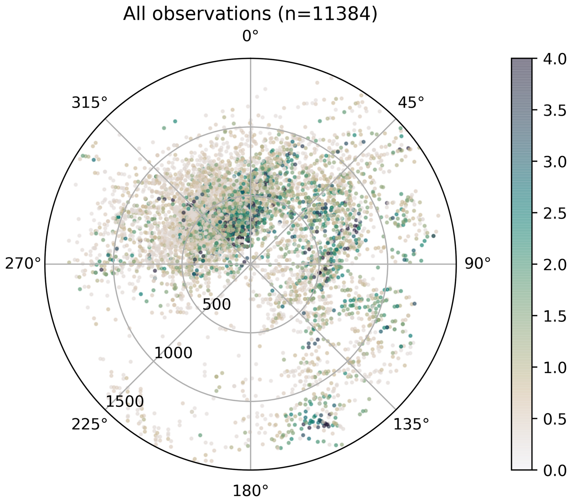
Figure 7 Lagrangian low-centric framework plot of hourly liquid-equivalent snowfall rates in units of m s⁻¹. The plot's center represents the tracked low-pressure center and each point represents 1 h of data from an ASOS station color-coded by the associated liquid-equivalent snowfall rate. Points are plotted with partial transparency to avoid obscuration.

The northwest quadrant typically contains the occluded front, and the northeast quadrant typically contains the upward-sloping frontal boundary ahead of the warm front. Frontogenesis is typically present in both the NE and NW quadrants (Novak et al., 2004). Additionally, for northeastern US winter storms the near-surface air in these quadrants is more often cold enough to support snow compared to the southwest quadrant cold frontal region that drapes further south and often yields rain.

The northeast quadrant, where frontogenesis typically occurs associated with the warm front, had the highest median and mean hourly snow rates among the four quadrants (see Table 6.1 in Tomkins, 2024a). The low-centric spatial distributions of liquid-equivalent snow rate align with our expectations given typical spatial patterns of large-scale lifting associated with different storm stages (Fig. 7). More active riming closer to the low, as found in Colle et al. (2014), would be consistent with heavier liquid water equivalents all other factors being equal, but ASOS data do not let us assess this hypothesis.

2.4 NASA IMPACTS airborne radar data

Vertical cross-sections collected from radars aboard the NASA ER-2 aircraft deployed during the NASA IMPACTS field campaign (McMurdie et al., 2022) illustrate typical vertical structures and horizontal wind profiles observed in winter storms. There were three radars (four frequencies in total) that sampled storms during the campaign: EXRAD, HIWRAP (two wavelengths), and CRS. EXRAD and HIWRAP are precipitation radars, while the CRS is a cloud radar. The cloud radar is more sensitive to smaller ice particles than the precipitation radars and has a smaller radar resolution volume size which is capable of observing finer-scale features (see Table 2 for details including the resolution of each radar at 10 km distance). The examples we present here have a reflectivity panel from the radar with the longest wavelength that was available (usually EXRAD but HIWRAP Ku-band if EXRAD was not available) as well as velocity and spectrum width from the shortest wavelength that was available (usually CRS but HIWRAP Ka-band if CRS was not available). Because the sensitivity is different for each radar (see Table 2) there is echo that is present in the velocity and spectrum width field that is not present in the reflectivity field. When available, velocity azimuth display (VAD) horizontal winds derived from the EXRAD scanning beam (Helms et al., 2020) are shown on the reflectivity cross-sections and summarized with contoured frequency by altitude diagrams (CFADs; Yuter and Houze, 1995) in terms of joint distributions of wind speed and height and wind direction and height. The latter are shown in polar coordinates.

Heymsfield et al. (1996)Li et al. (2016)McLinden et al. (2021)Oue et al. (2024)

Table 2 Band, frequency [GHz], sensitivity [dBZ] at 10 km, horizontal spatial resolution [m] at 10 km below the aircraft and vertical spatial resolution [m], and citation for radars deployed on the ER-2 aircraft during NASA IMPACTS. Band, frequency [GHz], sensitivity [dBZ] at 1 km, horizontal spatial resolution [m] at 10 km above the radar and vertical spatial resolution [m], and citation for KASPR deployed at Stony Brook University during NASA IMPACTS.

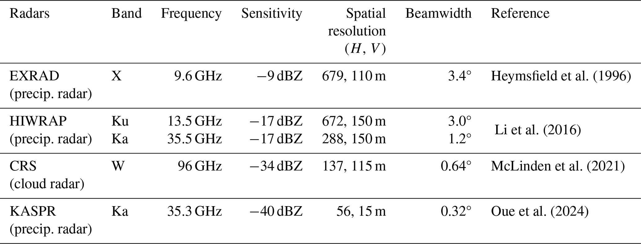
The ER-2 ground speed varies depending on wind speed and direction at flight level (i.e., slower in head winds and faster in tail winds). On average this value is ∼200 m s⁻¹. Actual ground speed values along each flight leg are converted to distance for plotting purposes. Section 3.2.2 shows five example transects during the NASA IMPACTS project. An additional 57 ER-2 transects with snow at the surface can be found in the Supplement.

The velocity and spectrum width fields are shown to provide additional context for the examples. The velocity field can be used to infer regions of rain versus snow, and Doppler spectrum width is a proxy for turbulence (Rauber and Nesbitt, 2018). To correct the spectrum width field to yield high-quality data, we use Eq. (7) in Heymsfield et al. (1996) to isolate the spectrum width of the hydrometeors and remove the spectrum width broadening caused by the aircraft speed. In some cases, this correction causes the spectrum width numeric value to become ≤0 m s⁻¹ (i.e., a nonphysical value; see blank echo in Fig. 15c), which is ignored in the plotting as it represents signal below the noise floor.

2.5 Stony Brook University Ka-band radar

Rapid-update range-height indicator (RHI) scans from the Ka-band (35 GHz) scanning fully polarimetric radar (KASPR) located at Stony Brook University further illustrate the evolution of enhanced features in a winter storm (Figs. 18 and 19). The data from the ground-based KASPR have finer vertical and horizontal spatial resolution than the ER-2 airborne radar data (Table 2).

The KASPR RHIs scan up and over the radar such that the azimuth angle of the radar beams within the RHI varies from ∼0–5° elevation angle in the southern part of the domain up to vertically pointing right over the radar and then back down to ∼5–10° elevation angle at the northern horizon in about 30 s.

When the radar beam is vertical or nearly vertical, the measured values of Doppler velocity and spectral width combine vertical air motions with precipitation particle fall speeds. When the radar beam is closer to horizontal, the measured motions are more indicative of the horizontal wind.

The effect of the changing component of the wind that is sampled as the radar beam elevation angle changes is particularly noticeable in the RHIs of Doppler velocity data (Figs. 18b and 19b). Plotted velocity values in a given layer tend to be strongest at the left and right edges of the RHI where the beam is more horizontal and peter out as the beam becomes more vertical near the center of the RHI plot. Whereas in the ER-2 radar vertically pointing data the Doppler velocity values were plotted with a range from −5 to 5 m s⁻¹, in these RHI plots, which are dominated by strong horizontal winds, the range plotted is −45 to 45 m s⁻¹. In the RHI plots, layers with low values of Doppler velocity indicate that the horizontal wind direction is close to perpendicular to the beam (i.e., in or out of the plane of the cross-section). A similar but less dramatic impact of beam angle on the measurements is apparent in the RHI spectral width plots. Although turbulence is usually close to isotropic, the combination of the air motion velocity spread with the strong signal from the often narrower precipitation fall speed spread tends to reduce the net spectral width magnitudes when the beam is pointed nearly vertical.

3 Results

The following results show that locally enhanced reflectivity features are not consistently related to heavy surface precipitation rates. Most of the time, precipitation rates are low, even when locally enhanced reflectivity features are present. Vertical cross-sections from airborne and ground-based radars illustrate that the local enhancements in reflectivity within snow are tilted and smeared on the way to the surface. The lack of vertical continuity of reflectivity enhancements in snow helps to explain the lack of relationship between local enhancements observed by operational scanning radars and heavier surface snow rates.

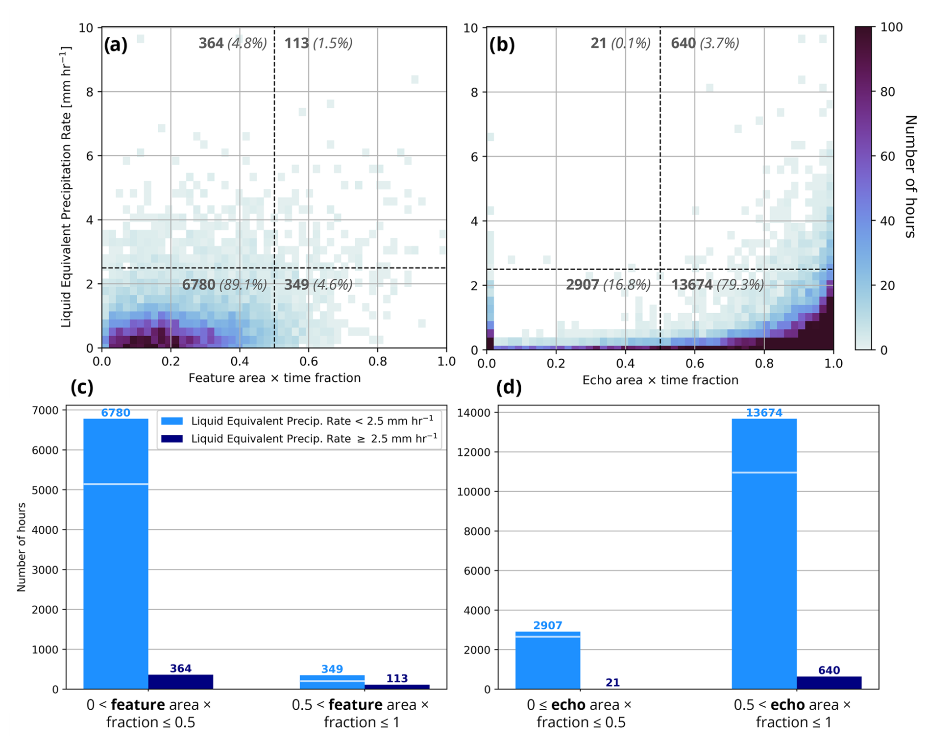
Figure 8 Joint distributions of the number of hours for (a) all-feature (faint + strong) area × time fraction and (b) all-echo (background + faint features + strong features) area × time fraction versus liquid-equivalent precipitation rate [mm h⁻¹] for snow observations. (c) Bar chart summarizing feature area × time fraction distribution in panel (a) and (d) a bar chart summarizing the echo area × time fraction distribution in panel (b). Light blue bars in panels (c) and (d) represent the liquid-equivalent precipitation rate < 2.5 mm h⁻¹, and dark blue bars represent liquid-equivalent precipitation rates ≥ 2.5 mm h⁻¹. Numbers of hours with liquid-equivalent precipitation rates < 1 mm h⁻¹ are annotated with horizontal lines on light blue bars in panels (c) and (d). Area × time fractions calculated with a 25 km radius and observations are paired with a 0 h lag. Zero feature area × time fraction observations in panels (a) and (c) are not shown. In panels (a) and (b) the 0.5 area × time fraction is annotated with a vertical black dashed line, and 2.5 mm h⁻¹ is annotated with a horizontal black dashed line. Bold annotated numbers in panels (a) and (b) indicate the number of hours in each quadrant, and italicized numbers indicate the percent of total observations in each quadrant. The feature area × time fraction in panels (a) and (c) has 7606 total hours compared to the all-echo area × time fraction in panels (b) and (d) with 17 242 h. The difference relates to the exclusion of hours with zero feature area × time fraction in panels (a) and (c).

3.1 Enhanced reflectivity features in horizontal maps and their relation to surface snowfall rates

Figure 8a shows the 2D distribution of all-feature (faint + strong) area × time fraction versus liquid-equivalent precipitation rate. The quadrants in Fig. 8a are summarized in a bar chart in Fig. 8c. Considering the previous literature focused on snow banding in winter storms, we were expecting to see a trend in the joint distribution indicating a relationship between increasing feature area × time fraction and increasing precipitation rate; however, this is not the case for the large sample size examined in this study. Most points (89.1 %) are clustered in the lower left box where both area × time fraction and precipitation rate are low. There are some observations where the area × time fraction and precipitation rate are high; however, they only account for ∼1.5 % of the observations when the feature area × time fraction is >0.

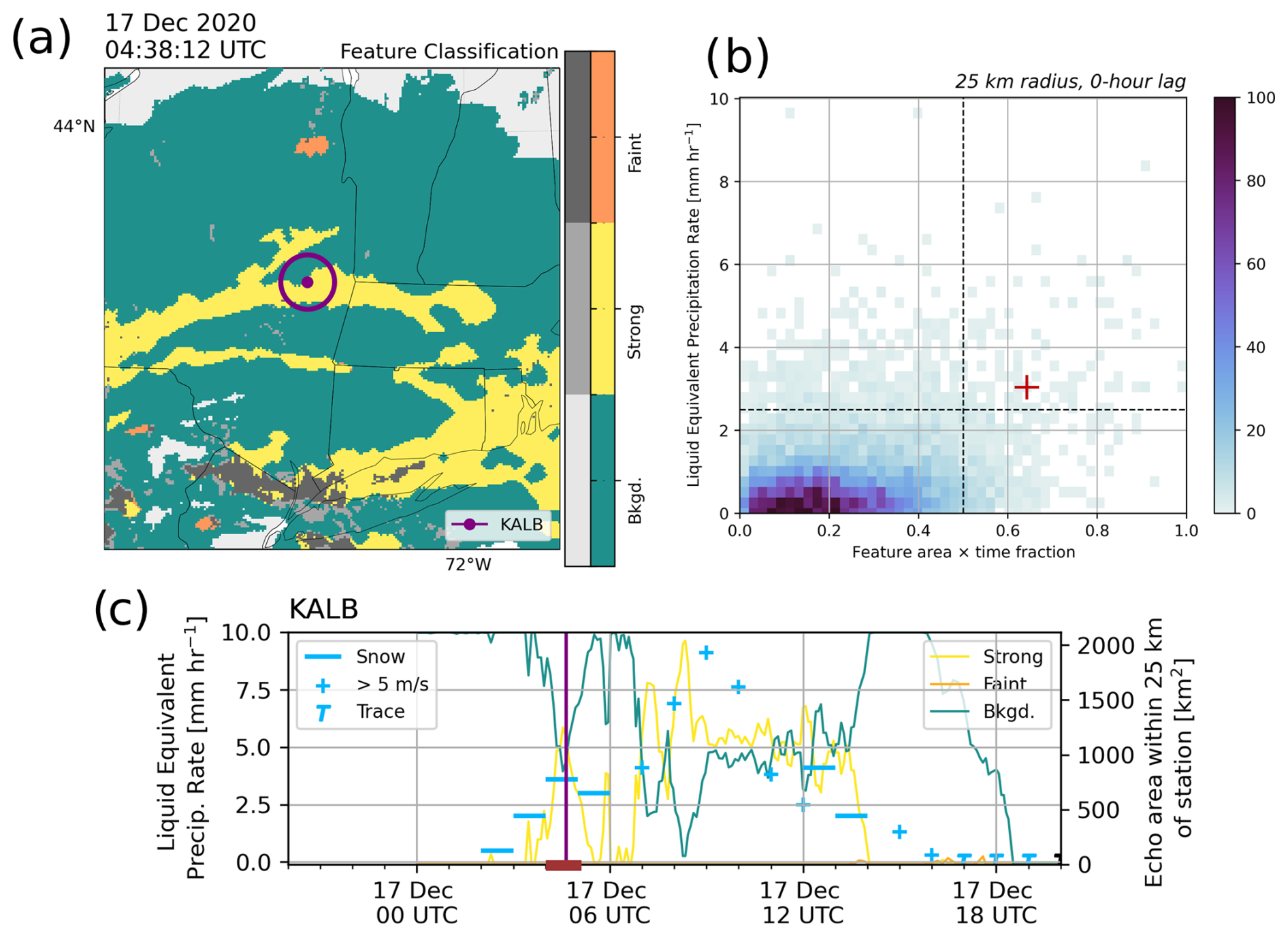
Figure 9 An example of when a heavy snow rate (≥2.5 mm h⁻¹) and high feature area × time fraction (>0.5) are observed over 1 h. (a) Feature detection field from a NEXRAD regional mosaic on 17 December 2020 at 04:38:12 UTC with the Albany, NY, ASOS station (KALB) and the 25 km radius annotated in purple. (b) 2D distribution from Fig. 8a with the specific hourly observation (04:00–05:00 UTC) annotated with a red plus sign. (c) Time series of the hourly precipitation rate over the entire event (16 December at 20:00 UTC to 17 December at 20:00 UTC) from KALB (blue annotations) and the area of each feature category within 25 km of KALB (yellow: strong area, orange: faint area, and teal: background area). In (a), gray colors indicate regions of partially melted or mixed precipitation. In (c), the purple vertical line indicates the time of the specific NEXRAD regional mosaic in (a), and the red bar on the x axis indicates the hour of observation at the red plus sign in (b). An animated version of this figure is available in the Video Supplement as Animation Fig. 9.

Heavy hourly snow rates in northeastern US winter storms are rare. Over all the hourly observations presented here, heavy snow rates (>2.5 mm h⁻¹) occurred <4 % of the time. This analysis indicates that anecdotal evidence from case studies in the literature showing a strong relation between heavier snow at the surface and enhanced reflectivity features aloft is not representative for a large sample size of 7606 h and 264 storms obtained over 11 years. Figure 8a and c indicate that equating snow bands with heavy snow will usually lead to overprediction of hourly snowfall rates. Our large sample size shows that three out of four times situations with feature area × time fractions > 0.5 have liquid-equivalent snow rates < 2.5 mm h⁻¹. More hours with heavy snow at the surface occurred associated with smaller feature areas (364 h) compared to larger feature areas (113 h).

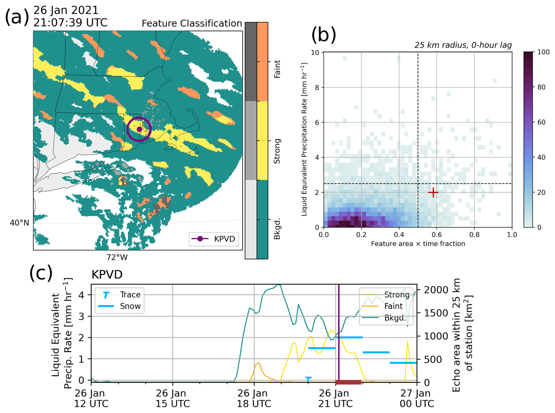
Figure 10 An example of when a low/moderate snow rate (<2.5 mm h⁻¹) and high feature area × time fraction (>0.5) are observed over 1 h. (a) Feature detection field from a NEXRAD regional mosaic on 26 January 2021 at 21:07:39 UTC with the Providence, RI, ASOS station (KPVD) and the 25 km radius annotated in purple. (b) 2D distribution from Fig. 8a with the specific hourly observation (21:00–22:00 UTC) annotated with a red plus sign. (c) Time series of the hourly precipitation rate over the entire event (26 January at 12:00 UTC to 27 January at 00:00 UTC) from KPVD (blue annotations) and the area of each feature category within 25 km of KPVD (yellow: strong area, orange: faint area, and teal: background area). In (a), gray colors indicate regions of partially melted or mixed precipitation. In (c), the purple vertical line indicates the time of the specific NEXRAD regional mosaic in (a), and the red bar on the x axis indicates the hour of observation at the red plus sign in (b). An animated version of this figure is available in the Video Supplement as Animation Fig. 10.

Since locally enhanced reflectivity features are not particularly helpful in identifying regions of heavy snow rates, we calculate the area × time fraction for all echo areas to see if there are patterns present (Fig. 8b and d). The patterns in this 2D distribution indicate that heavy snow rates (>2.5 mm h⁻¹) are more common when there is a large echo area × time fraction (i.e., there is a lot of echo surrounding the station for a longer duration). This suggests that it is more useful to focus on the duration of all echoes over a location rather than the size, duration, and location of just the locally enhanced reflectivity features (i.e., snow bands) to deduce where higher snowfall accumulations may occur. The distribution of snowfall rates has a strong skewness to low values; 75 % of the time it is snowing at a rate no more than 1 mm h⁻¹. So even if there is an enhanced reflectivity feature area it is more likely associated with a low snow rate than a heavy snow rate.

To provide context for the joint frequency distribution, we present representative examples of each quadrant in Fig. 8a. The first is an example when a high feature area × time fraction and heavy snowfall are observed over 1 h (Fig. 9). Figure 9a illustrates a large, strong feature over the Albany, NY, ASOS station which contributes to a feature area × time fraction of 0.62 over the hour and coincides with an hourly liquid-equivalent snowfall rate of 3.6 mm h⁻¹. Later in this event, there are several hours at this station that were not included in our analysis because the wind speed was too high (blue plus signs in Fig. 9c). The scenario of high feature area and heavy snowfall occurs in only 1.5 % of hours in our dataset. In this specific example, the feature resembles a primary band and is likely forced by frontogenesis.

The second example is from an event on 26 January 2021 where several strong and faint features are moving through the region (Fig. 10a). In the snapshot in Fig. 10a, there is a strong feature over the Providence, RI, ASOS station which contributes to a feature area × time of 0.58 over the hour (Fig. 10). While the feature area × time fraction is high (>0.5) in this example, the snow rate is 2 mm h⁻¹ (Fig. 10c). Scenarios with a high feature area × time fraction and a low/moderate snow rate represent 4.6 % of hours in our dataset.

The next example from 2 February 2021 represents the most common occurrence in our dataset where a low feature area × time fraction and a low/moderate snow rate are observed over the hour. This example from Lebanon, NH, shows only a small faint object in the vicinity of the ASOS station and has a feature area × time fraction of 0.2 over the hour and a snow rate of 1.3 mm h⁻¹ (Fig. 11). For the remainder of the event there are no features in the vicinity of the ASOS station and the snow rate remains low/moderate (Fig. 11c). Scenarios where the feature area × time fraction is low and the snow rate is low account for 89 % of observations.

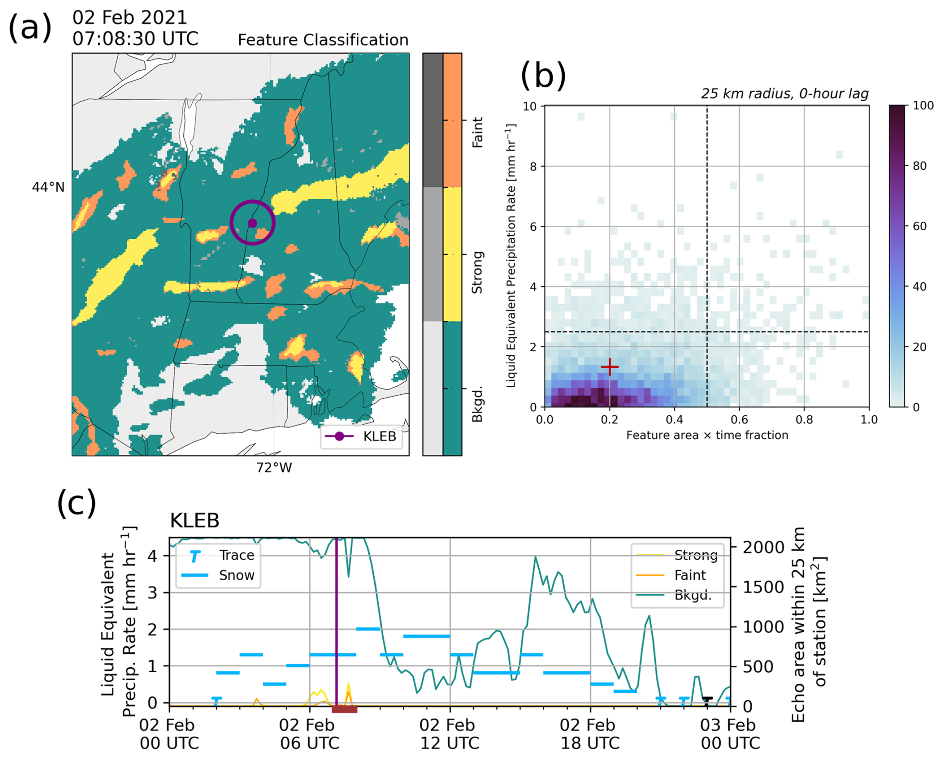
Figure 11 An example of when a low/moderate snow rate (<2.5 mm h⁻¹) and low feature area × time fraction (≤0.5) are observed over 1 h. (a) Feature detection field from a NEXRAD regional mosaic on 2 February 2021 at 07:08:30 UTC with the Lebanon, NH, ASOS station (KLEB) and the 25 km radius annotated in purple. (b) 2D distribution from Fig. 8a with the specific hourly observation (07:00–08:00 UTC) annotated with a red plus sign. (c) Time series of the hourly precipitation rate over the entire event (2 February at 00:00 UTC to 3 February at 00:00 UTC) from KLEB (blue annotations) and the area of each feature category within 25 km of KLEB (yellow: strong area, orange: faint area, and teal: background area). In (a), gray colors indicate regions of partially melted or mixed precipitation. In (c), the purple vertical line indicates the time of the specific NEXRAD regional mosaic in (a), and the red bar on the x axis indicates the hour of observation at the red plus sign in (b). An animated version of this figure is available in the Video Supplement as Animation Fig. 11.

Lastly, we have an example when the feature area × time fraction is low but the snow rate is heavy, which occurs in 4.8 % of our observations. This example from Worcester, MA, shows 1 h where the liquid-equivalent precipitation rate was 9.7 mm h⁻¹ but the feature area × time fraction was only 0.12 (Fig. 12). There are a few faint features in the area, but overall the echo is patchy. The all-echo area × time fraction was 0.9. The time series shows that there are several times in this event where the snow rate was heavy but there were few or no features present over the station. Scenarios with a small feature area × time fraction commonly have a long duration of background echo rather than mostly locally enhanced reflectivity features. It is also possible that in this case that the snowstorm is shallow and the radar beam height is above any locally enhanced features.

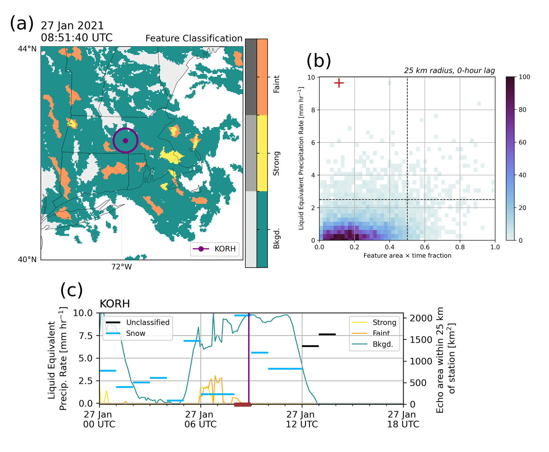
Figure 12 An example of when a heavy snow rate (≥2.5 mm h⁻¹) and low feature area × time fraction (≤0.5) are observed over 1 h. (a) Feature detection field from a NEXRAD regional mosaic on 27 January 2021 at 08:51:40 UTC with the Worcester, MA, ASOS station (KORH) and the 25 km radius annotated in purple. (b) 2D distribution from Fig. 8a with the specific hourly observation (08:00–09:00 UTC) annotated with a red plus sign. (c) Time series of the hourly precipitation rate over the entire event (27 January at 00:00 UTC to 27 January at 18:00 UTC) from KORH (blue annotations) and the area of each feature category within 25 km of KORH (yellow: strong area, orange: faint area, and teal: background area). In (a), gray colors indicate regions of partially melted or mixed precipitation. In (c), the purple vertical line indicates the time of the specific NEXRAD regional mosaic in (a), and the red bar on the x axis indicates the hour of observation at the red plus sign in (b). An animated version of this figure is available in the Video Supplement as Animation Fig. 12.

3.1.1 Sensitivity tests

We tested the sensitivity of the results in Fig. 8 by varying various thresholds used in the calculations, and these adjustments did not appreciably change our results (Figs. 5.10-5.14 in Tomkins, 2024a). We varied the radius around the ASOS station to 12.5, 25, and 50 km to account for the horizontal advection of snow, the time lag between the radar and ASOS observations (0, 1, and 2 h), and the number of hours of precipitation accumulation (1, 2, and 3 h). We also subset by radar beam altitude above the ASOS station and the percent of mixed precipitation echo removed over the hour. For example, applying thresholds based on the average beam height of the radar echo changed the fraction of hours in the high area × time fraction–heavy snow rate category to 1.8 % for ≤1000 m, 1.7 % for ≤2000 m, and 1.5 % for ≤3000 m. While these sensitivity tests yielded slightly different numbers for each quadrant in the joint distributions of feature area × time fraction versus liquid-water-equivalent precipitation rate, the key findings from Fig. 8 are robust relative to the tested variations.

3.2 Vertical structures in reflectivity are tilted and smeared

The lack of relationship between ground-based scanning-radar-observed locally enhanced reflectivity features and snow rates indicates that the radar observations above the surface are not necessarily consistent with snow rates observed directly below at the surface. As discussed in Sect. 1, there are several factors that complicate the relationship between reflectivity and snowfall rate compared to reflectivity and rain rate: changes in radar reflectivity in snow (especially aggregation and partial melting) do not necessarily equate to changes in ice mass (Table 1); slow fall speeds of snow yield time for advection of snow over tens of kilometers by horizontal winds as it falls to the surface, and there is a large spread in observed values for a given IWC and its associated radar reflectivity.

High-spatial-resolution vertical cross-sections of radar data from winter storms indicate that snow rarely falls straight down to the surface. Locally enhanced reflectivity features in snow tend to be tilted and smeared by the wind shear (changes in the wind speed and direction with height) between echo top and the surface. In the following two sections, we feature examples of high-vertical-resolution cross-sections within snowstorms that illustrate the lack of vertical column continuity in locally enhanced reflectivity.

3.2.1 Vertical structures observed by airborne radar data

As aircraft equipped with vertically pointing radar fly along, they obtain a slice through the atmosphere. For the NASA ER-2, which has a ground speed of ∼200 m s⁻¹, each 50 km in distance along the leg represents 5.6 min of flight time. Adjacent portions along the track can be considered to be coincident in time within a few minutes.

The first example from 5 February 2020 in the Midwest illustrates several types of variations in the structures in the reflectivity field (Fig. 13). At the beginning of the transect, when the aircraft is traveling from the edge of the echo in the regional map (northern Illinois; Fig. 13d), the vertical cross-sections indicate that the echo aloft is not reaching the surface (0–40, 0–1 km altitude in Fig. 13a). At ∼90 km along the flight track, there are regions where there is echo reaching the surface but “holes” in the echo aloft. Other regions along the cross-section show consistent echo through the vertical column and indicate lots of wind shear illustrated by the wind barbs and bends in the local variations of the reflectivity field itself (i.e., 125–175 km in Fig. 13a). The wind barbs in the VAD profiles indicate the direction and speed that the wind is coming from and correspond well to the patterns in the reflectivity field. The CFADs summarize the distributions with height of the direction and speed of the winds in the VAD profiles along the flight leg. It is important to note that the cross-sections are plotted in a 3:1 aspect ratio (3 units in vertical to 1 unit in horizontal distance) so features that are tilted appear to be more vertical in the plots (see triangle icons next to Fig. 13c for visualization). An example transect showing a comparison between a 1:1 aspect ratio and a 3:1 aspect ratio is available in the Supplement. CFADs of the wind speed (Fig. 13e) and wind direction (Fig. 13f) along the track indicate considerable vertical wind shear. Horizontal wind speeds reach around 30 m s⁻¹ at 5 km altitude near the top of the echo. The wind direction at 5 km altitude is roughly perpendicular to the direction the aircraft is traveling, indicating that snow particles forming aloft will be transported out of the cross-section as they descend to the surface (Fig. 13b and c). While the human eye would like to connect structures through the entire depth of the echo, this is deceptive as spatial patterns in the lower portion of the echo are the result of features at higher altitudes that are unseen (upwind and perpendicular) in the depicted cross-section.

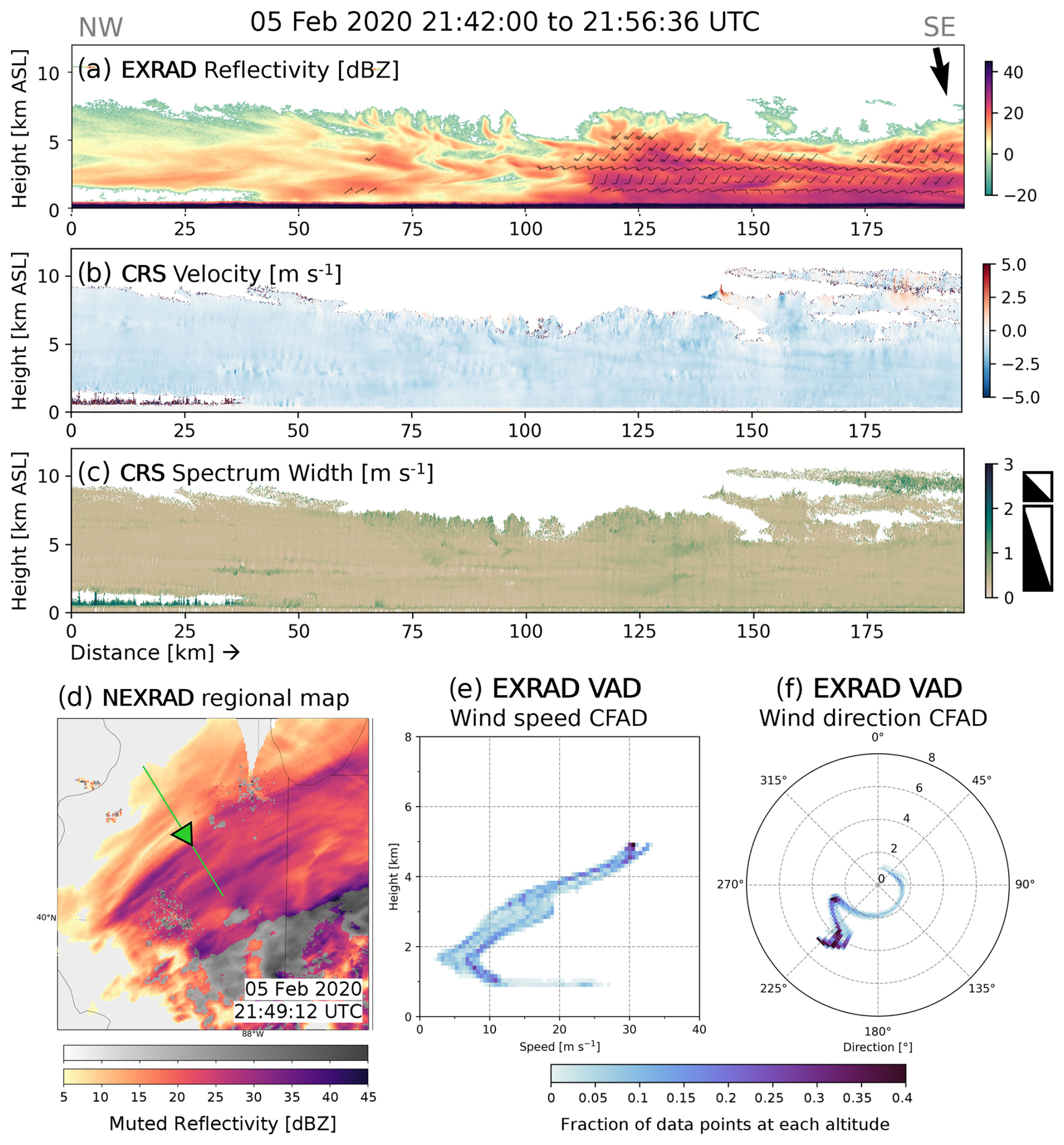
Figure 13 Vertical cross-section from 5 February 2020 at 21:42:04 to 21:56:44 UTC of (a) reflectivity [dBZ] from the NASA EXRAD radar (nadir beam) and VAD winds derived from the EXRAD radar (scanning beam), (b) velocity [m s⁻¹], and (c) spectrum width [m s⁻¹] from the NASA CRS cloud radar. All vertical cross-sections are plotted with a 3:1 aspect ratio. Triangle icons next to (c) illustrate a 45° angle in a 1:1 and 3:1 aspect ratio. (d) Corresponding NEXRAD regional map of image-muted reflectivity [dBZ] with the ER-2 flight path in green; the arrowhead denotes the direction and location of the aircraft at the time of the region map. CFADs of (e) wind speed and (f) wind direction of VAD winds in (a). Wind direction CFAD indicates the direction the wind is coming from and is plotted in polar coordinates where the angle represents the direction and each radius represents the altitude (0 km at the center). The black arrow in (a) indicates the compass direction of the aircraft during the transect.

The next example from 7 February 2020 shows a transect over New York (Fig. 14). In this example, the reflectivity is more uniform compared to the previous example (Fig. 14a). The aircraft is traveling westward from a region of higher reflectivity in central New York to a region of weaker reflectivity in western New York (Fig. 14a and d). This case was examined in Colle et al. (2023) for the lack of snow banding despite considerable frontogenesis being present (values > 10 K (100 km)⁻¹ (3 h)⁻¹). The CFADs of the wind speed and direction from the transect indicate speed shear and some directional shear (Fig. 14e and f). Similar to Fig. 13, the wind direction is roughly perpendicular to the direction the aircraft is flying, indicating that the particles forming aloft are advected away from the flight path – and hence the vertical plane of the cross-section – as they fall (Fig. 14).

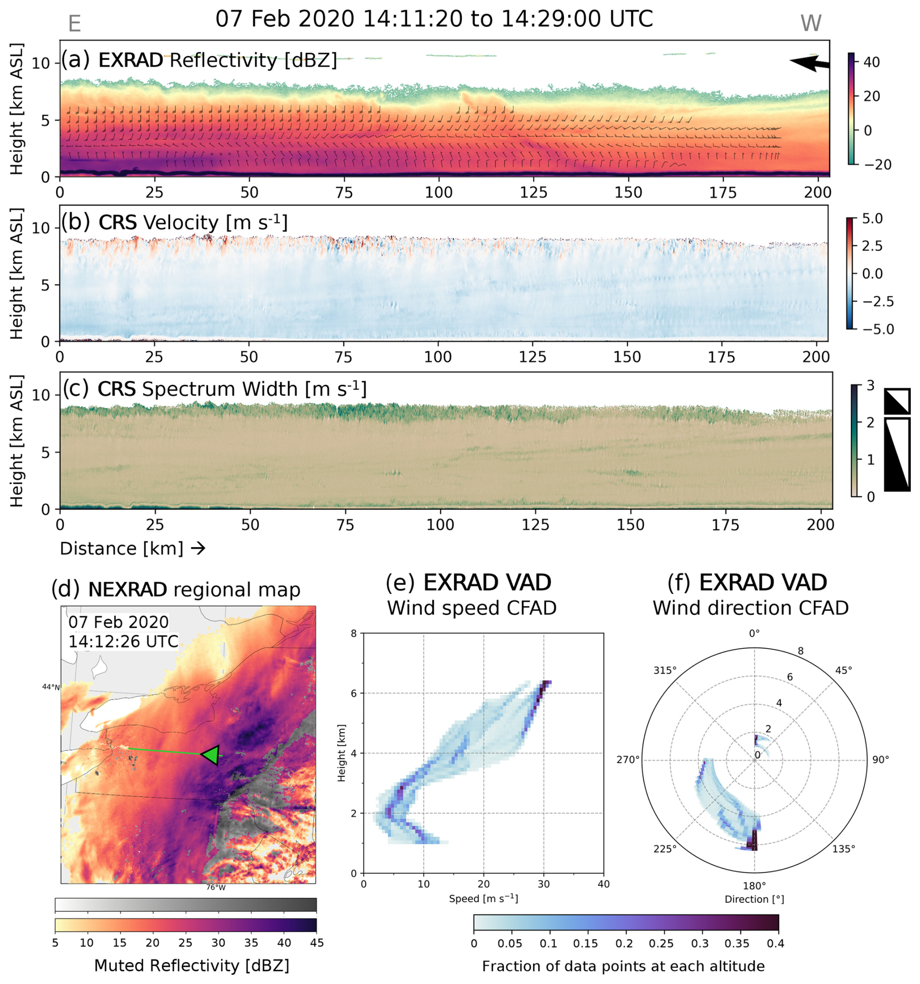
Figure 14 Vertical cross-section from 7 February 2020 at 14:11:20 to 14:29:00 UTC of (a) reflectivity [dBZ] from the NASA EXRAD radar (nadir beam) and VAD winds derived from the EXRAD radar (scanning beam), (b) velocity [m s⁻¹], and (c) spectrum width [m s⁻¹] from the NASA CRS cloud radar. All vertical cross-sections are plotted with a 3:1 aspect ratio. Triangle icons next to (c) illustrate a 45° angle in a 1:1 and 3:1 aspect ratio. (d) Corresponding NEXRAD regional map of image-muted reflectivity [dBZ] with the ER-2 flight path in green; the arrowhead denotes the direction and location of the aircraft at the time of the region map. CFADs of (e) wind speed and (f) wind direction of VAD winds in (a). Wind direction CFAD indicates the direction the wind is coming from and is plotted in polar coordinates where the angle represents the direction and each radius represents the altitude (0 km at the center). The black arrow in (a) indicates the compass direction of the aircraft during the transect.

An example from 23 January 2023 shows a case where the aircraft flew parallel to strong, banded features in Maine and New Hampshire (Fig. 15). The reflectivity cross-section shows ice streamers that are tilted as they approach the surface. The tops of the ice streamers are likely generating cells associated with overturning circulations near cloud top (Fig. 15a). The velocity and spectrum width cross-sections indicate some overturning circulations near echo top between 150–200 km along the flight track (Fig. 15b and c). A nonuniform beam filling (NUBF) correction was applied to the velocity data and the circulation features show up in all wavelengths, indicating that these velocity features are not NUBF (Gerald Heymsfield and M. Walker McLinden, personal communication, July 2023). As particles originating in the generating cells descend to the surface in ice streamers there are corresponding downward local enhancements in velocity (Fig. 15b) and locally higher spectral width values (Fig. 15c). The aircraft is flying from NE to SW (Fig. 15d) and the horizontal winds in the layer between 5 and 3 km altitude are from the SSW (Fig. 15a). Below 3 km altitude, winds turn and move from the N to ENE. The ice streamer advection in the 5 to 3 km layer is close to being aligned with the flight path. This yields an aircraft radar cross-section that is more representative of the ice streamer's shape (Fig. 15a) than the previous examples where the ice streamer advection was more perpendicular to the flight path (Figs. 13a and 14a).

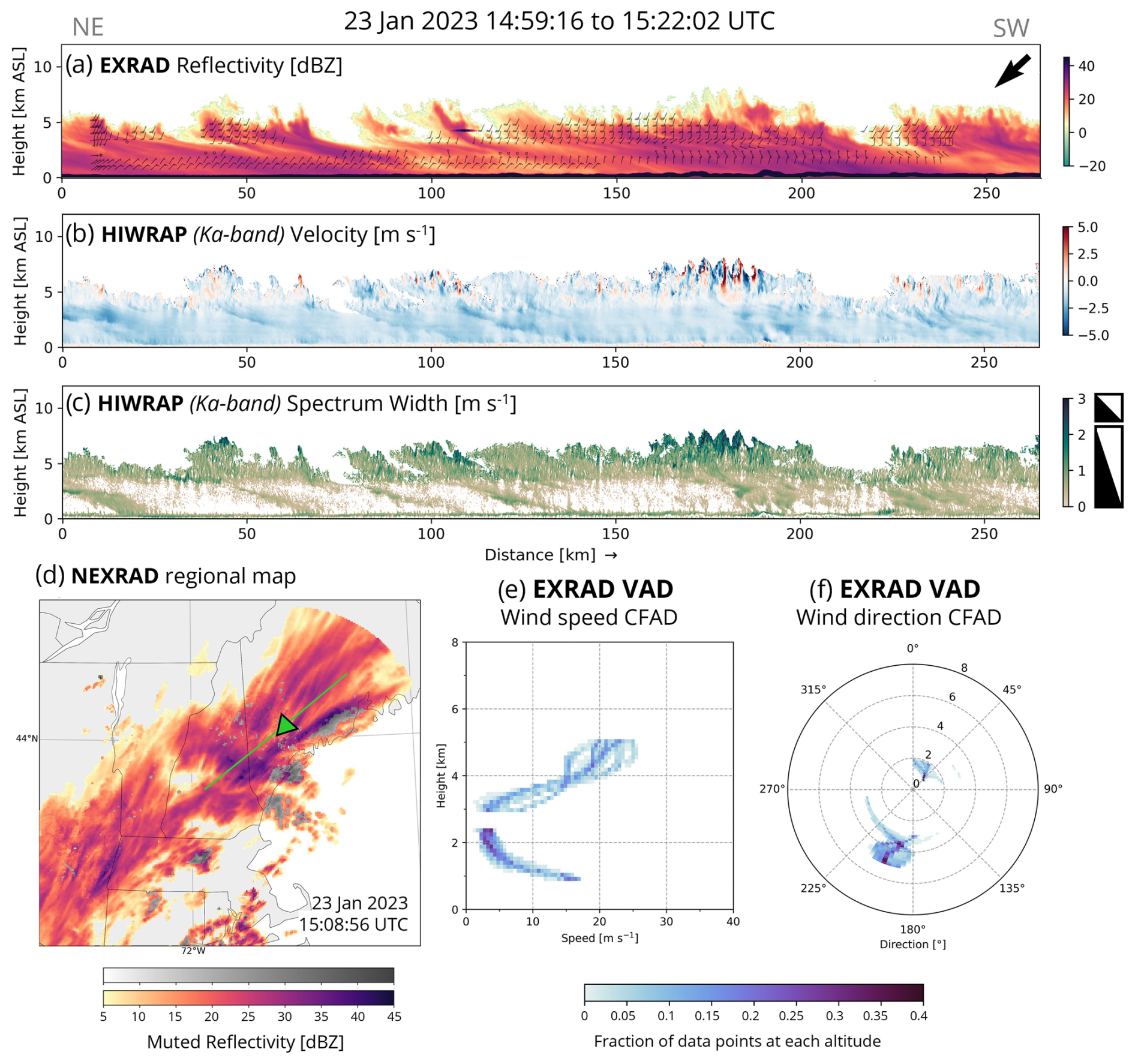
Figure 15 Vertical cross-section from 23 January 2023 at 14:59:16 to 15:22:02 UTC of (a) reflectivity [dBZ] from the NASA EXRAD radar (nadir beam) and VAD winds derived from the EXRAD radar (scanning beam), (b) velocity [m s⁻¹], and (c) spectrum width [m s⁻¹] from the NASA HIWRAP (Ka-band) radar. All vertical cross-sections are plotted with a 3:1 aspect ratio. Triangle icons next to (c) illustrate a 45° angle in a 1:1 and 3:1 aspect ratio. (d) Corresponding NEXRAD regional map of image-muted reflectivity [dBZ] with the ER-2 flight path in green; the arrowhead denotes the direction and location of the aircraft at the time of the region map. CFADs of (e) wind speed and (f) wind direction of VAD winds in (a). Wind direction CFAD indicates the direction the wind is coming from and is plotted in polar coordinates where the angle represents the direction and each radius represents the altitude (0 km at the center). The black arrow in (a) indicates the compass direction of the aircraft during the transect.

The remaining examples do not have VAD horizontal wind data available. We include a panel of the feature detection field instead for context. Figure 16 shows an example from a 300 km long flight track that flew over some faint enhanced reflectivity features in the Gulf of Maine. The regional radar reflectivity indicates that this storm had weaker and more patchy echo compared to the previous examples (Fig. 16d). The radar cross-sections show shallower echo tops (∼5 km altitude) compared to the previous examples. Between 125 and 175 km along the flight track, enhanced reflectivity features tilt to the right and then to the left. There are weak echo holes throughout the cross-section.

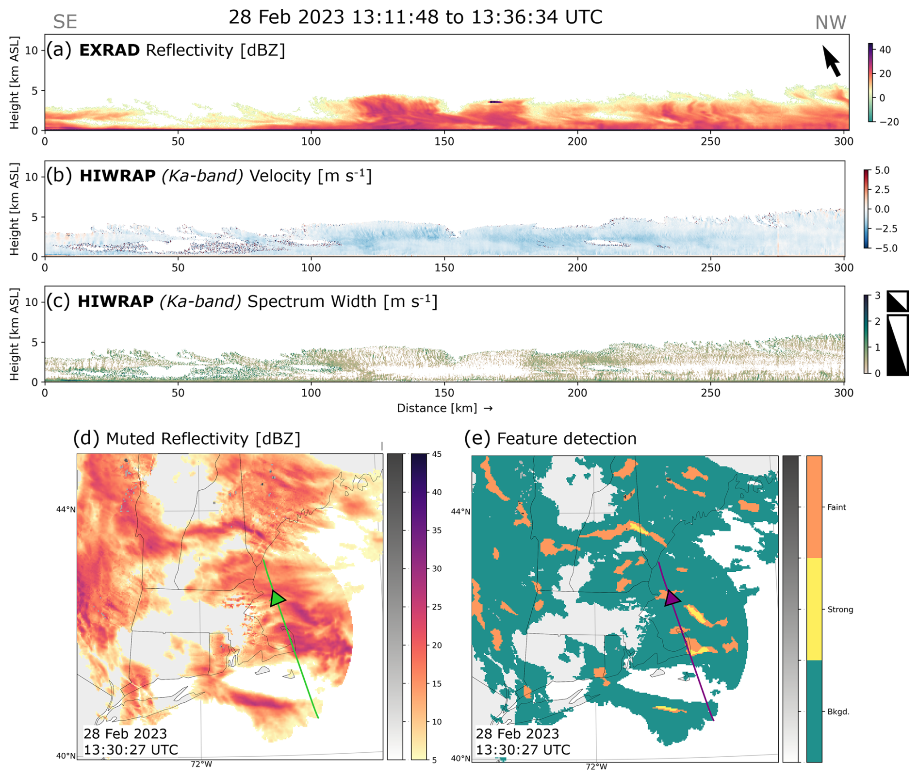
Figure 16 Vertical cross-section from 28 February 2023 at 13:11:48 to 13:36:34 UTC of (a) reflectivity [dBZ] from the NASA EXRAD radar (nadir beam), (b) velocity [m s⁻¹], and (c) spectrum width [m s⁻¹] from the NASA HIWRAP (Ka-band) radar. All vertical cross-sections are plotted with a 3:1 aspect ratio. Triangle icons next to (c) illustrate a 45° angle in a 1:1 and 3:1 aspect ratio. Corresponding NEXRAD regional map of (d) image-muted reflectivity [dBZ] with the ER-2 flight path in green and (e) feature detection classification with the ER-2 flight path in purple; the arrowhead denotes the direction and location of the aircraft at the time of the region map. The black arrow in (a) indicates the compass direction of the aircraft during the transect.

Figure 17 shows an example from 17 February 2022 when the aircraft sampled a faint, banded feature over Lake Michigan (200–215 km along flight track). The flight track began over central Indiana (southeast) over surface rainfall, which transitioned to surface snow at ∼48 km along the flight track. This surface rain portion of the flight track is depicted as an image-muted area in gray in Fig. 17d, and it has a radar bright band and high Doppler velocities and spectral width in the rain layer between 0–48 km (Fig. 17a–c). Along the flight track within the snow layer between 6 and 2.5 km altitude, locally enhanced reflectivity features in snow tend to tilt to the right (towards northwest). At the northwest end of the flight track when the aircraft approaches the faint enhanced feature in the map (Fig. 17e), there is a layer of locally enhanced reflectivity at ∼2.5 km altitude between 150–250 km (Fig. 17a) with weaker to no echo below it. It is possible that the faint feature in the map manifests as the scanning radar intersects part of this elevated region of enhanced reflectivity.

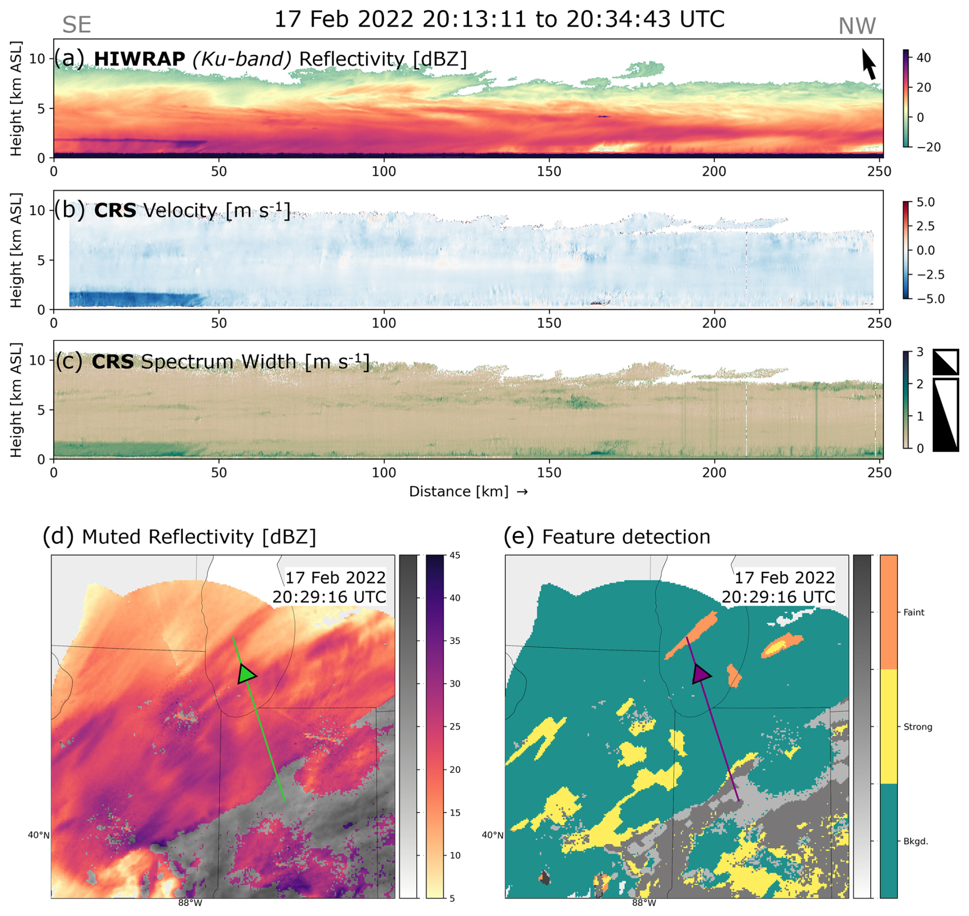
Figure 17 Vertical cross-section from 17 February 2022 at 20:13:11 to 20:34:43 UTC of (a) reflectivity [dBZ] from the NASA HIWRAP (Ku-band) radar, (b) velocity [m s⁻¹], and (c) spectrum width [m s⁻¹] from the NASA CRS cloud radar. All vertical cross-sections are plotted with a 3:1 aspect ratio. Triangle icons next to (c) illustrate a 45° angle in a 1:1 and 3:1 aspect ratio. Corresponding NEXRAD regional map of (d) image-muted reflectivity [dBZ] with the ER-2 flight path in green and (e) feature detection classification with the ER-2 flight path in purple; the arrowhead denotes the direction and location of the aircraft at the time of the region map. The black arrow in (a) indicates the compass direction of the aircraft during the transect.

As part of this study, we examined all transects from the NASA IMPACTS campaign, which included snow reaching the surface. In addition to Figs. 13–17 there are 53 additional transects which are shown in the Supplement. IMPACTS flight legs that pass over regions with just rain at the surface are not included. For each transect in the Supplement, we present the reflectivity, velocity, spectrum width, and linear depolarization ratio (LDR) fields from the instrument with the shortest wavelength available (usually CRS but occasionally HIWRAP Ku-band) and the reflectivity field from the instrument with the longest wavelength available (usually EXRAD but occasionally HIWRAP Ka-band). We include snapshots of the NEXRAD regional maps to provide context for the transects. If available, we include the VAD winds on the EXRAD reflectivity transects and CFADs of wind speed and direction to summarize. Each transect in the Supplement is annotated with a vertical dashed black line which annotates where the enhanced reflectivity features are in the regional maps. Full details are available in the Supplement. The additional examples shown in the Supplement are consistent with the findings illustrated in Figs. 13–17.

3.2.2 Sequences of vertical structures observed from ground-based radar data

Fast-update RHIs from ground-based radar can obtain individual vertical cross-sections that complete in tens of seconds and yield sequences of RHIs that can address storm evolution along the vertical plane at timescales < 1 min. Within snowstorms noticeable structural changes along a given vertical cross-section from a combination of storm advection and evolution usually have timescales of several minutes or more.

We show examples of fast-update RHIs from the Stony Brook University KASPR from a storm that spanned 40 h from 31 January to 2 February 2021. An animation of the sequence of RHIs for the full storm period, as well as two 2 h periods corresponding to Figs. 18 and 19, is included in the Video Supplement. While RHIs have often been obtained by research radars in winter storms, this is one of the few examples with an update fast enough to discern how a storm's individual features change with time along the plane of the RHI vertical cross-section.

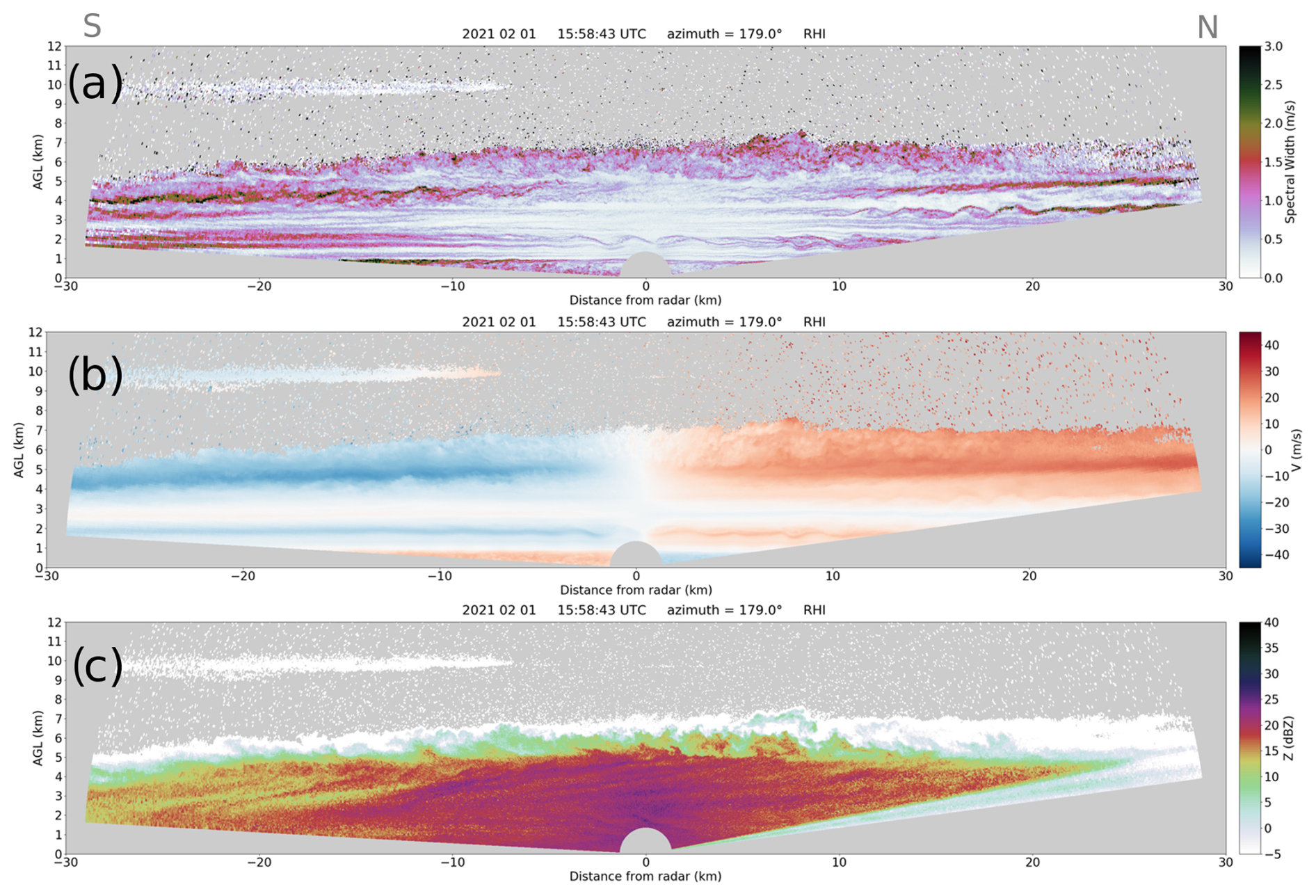
Figure 18 (a) Spectrum width [m s⁻¹], (b) Doppler velocity [m s⁻¹], and (c) reflectivity [dBZ] RHIs from KASPR at Stony Brook University at 15:58:42 UTC on 1 February 2021. RHIs are scanned up and over the radar (at 0 km on the x axis). The radar beam is partially blocked near the edge of the scan on the right side. The figure is plotted in a 1:1 aspect ratio. An animated version of this figure between 15:05–17:03 UTC is available in the Video Supplement as Animation Fig. 18. An animation of the full storm is available in the Video Supplement as Animation Figs. 18–19-full.

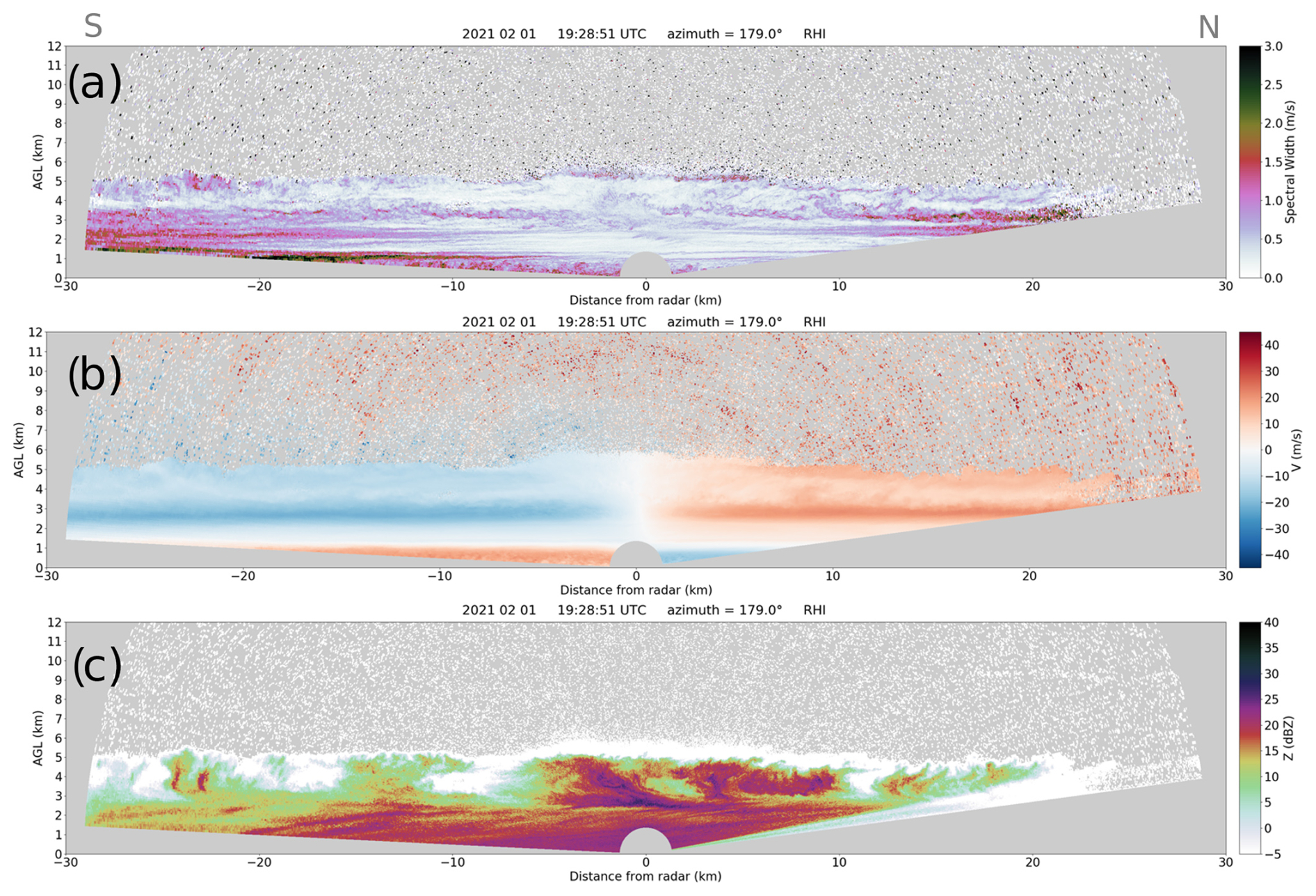
Figure 19 (a) Spectrum width [m s⁻¹], (b) Doppler velocity [m s⁻¹], and (c) reflectivity [dBZ] RHIs from KASPR at Stony Brook University at 19:28:51 UTC on 1 February 2021. The RHIs are scanned up and over the radar (at 0 km on the x axis). The radar beam is partially blocked near the edge of the scan on the right side. The figure is plotted in a 1:1 aspect ratio. An animated version of this figure between 18:24–20:25 UTC is available in the Video Supplement as Animation Fig. 19. An animation of the full storm is available in the Video Supplement as Animation Figs. 18–19-full.

During the 31 January to 2 February 2021 storm, the KASPR scan strategy consisted of the following sequence that was repeated every 15 min: plan position indicator (PPI) at 15° elevation angle (50 s), set of eight cross-band RHIs (6 min), vertically pointing mode (2 min), set of eight cross-band RHIs (6 min). KASPR's mechanical antenna took a few seconds to reverse direction at the end of each RHI sweep. Each single RHI sweep took ∼30 s (scan rate of 4–6 s per degree) and can be considered to be similar to a snapshot.

Below the cloud-top generating cells in the first example at 15:58 UTC on 1 February 2021 (Fig. 18), the reflectivity enhancements bend with the wind patterns, which switch direction several times through the depth of the echo. The spectrum width is enhanced at echo top associated with overturning circulations within the generating cells (Fig. 18a). Other narrow layers of enhanced spectrum width are present at several altitudes including close to the surface (Fig. 18a). The Doppler velocity field helps to illustrate the horizontal winds and how they vary with height (Fig. 18b). Near cloud top the winds are left to right, corresponding to a wind with a southerly component (wind coming from the south). In the layer between 2.3 and 3 km a.g.l. the magnitude of the velocity is near zero, which indicates that the wind direction is pointing perpendicular to the radar beam. Between the surface and 1 km altitude there is shift in the wind direction to a wind with a north component illustrated by the change in sign of the Doppler velocity. The reflectivity field shows a lot of detail, including ice streamers that manifest from the overturning circulations near echo top (Fig. 18c). The ice streamer features become tilted and smeared on the way to the surface, likely due to the distinct layers in the wind profile illustrated in the Doppler velocity field. In this example, the cross-sections are plotted in a 1:1 aspect ratio so the tilt of the features is shown as it occurs in reality. As the snow particles within the enhanced reflectivity features descend in the storm they move much faster sideways than they do vertically. Unless the horizontal winds are very weak, snow cannot fall “straight” down in a column. It is also important to note that the precipitation particles are not all falling within the plane of the RHI. In particular, reflectivity values at altitudes with layers of near-zero Doppler velocity are potentially either moving in or out perpendicular to the cross-section. Whenever the wind direction changes between layers, the trajectories of individual precipitation particles turn with the wind, yielding complex 3D trajectories between their origin near cloud top and the surface.

In the second example a few hours later at 19:28 UTC (Fig. 19), the cloud-top generating cells are still evident and the bending of the enhancements to the left then the right is more evident. The echo is slightly shallower overall and the reflectivity field is more variable near cloud top, varying from close to the minimum detectable echo at −5 dBZ to close to 25 dBZ (Fig. 19c). There is some locally higher spectral width and likely turbulence close to 5 km altitude near echo top at the location of generating cells near −24 to −26 km and directly above the radar near 0 km (Fig. 19a). There is a discontinuity in the direction of tilt of ice streamers within the reflectivity field at about 3 km altitude from toward the right (north) to toward the left (south), corresponding to the wind shift observed in the Doppler velocity field (Fig. 19b). Similar to 15:58 UTC, the wind also sharply shifts direction to a north wind at about 1 km altitude above the surface.

The aircraft radar cross-sections from the NASA IMPACTS campaign and RHI scans from KASPR illustrate how features in the snow reflectivity field are tilted and smeared in winter storms. The lack of vertical column continuity of enhanced reflectivity aloft to the surface complicates the interpretation of reflectivity from PPI scanning radar in snow and provides a physical explanation for why we are not seeing a strong relationship between enhanced reflectivity aloft and snow rates at the surface.

4 Conclusions

Determining where and when heavy snow is likely to occur in northeastern US winter storms is both a high-impact and thorny problem. We analyzed observations of a large sample of snowstorm events with negligible orographic forcing in the northeastern US to improve the understanding of how hourly snowfall rates relate to structural characteristics of these winter storms. Data are from 264 storm days over 11 years (2012–2023), which yielded over 7500 time–spatial matched pairs of hourly surface observations and radar data that included enhanced reflectivity features in snow. Motivated by previous work, we examined mesoscale snow bands (locally enhanced reflectivity features) – a “prime suspect” in the occurrence of heavy snowfall. Most of the time in northeastern US winter storms, the snow rates are low (75 % of hours had liquid-equivalent snow rates less than 1 mm h⁻¹; see the horizontal annotations on light blue bars in Fig. 8c and d) and only 4% of hours had heavy snow rates > 2.5 mm h⁻¹ (Fig. 8). Our dataset excludes conditions with high surface winds (>5 m s⁻¹) so these data are representative of non-blizzard conditions. Consistent with previous work, higher snow rates are more likely to occur closer to the low-pressure center (within 250–500 km), especially in the northwest and northeast quadrants of the storm (Fig. 7).

Regional radar mosaics over the northeastern US were created from the NWS NEXRAD network that included output from two new objective image processing methods developed specifically for this work: the removal of mixed precipitation areas (Tomkins et al., 2022) and the objective identification of locally enhanced reflectivity features in snow (Tomkins et al., 2024a). Potential associations between radar reflectivity structures in the vicinity of ASOS stations and hourly snow rates were examined in terms of incidence of locally enhanced reflectivity features as well as all snow echo.

Evidence from our analysis demonstrates that operational PPI scanning-radar-observed locally enhanced reflectivity features within these snowstorms are not consistently associated with heavy snowfall rates at the surface. When enhanced reflectivity features pass over a location (area × time fractions > 0.5), only one out of four occurrences have hourly heavy surface snow liquid-water equivalents (≥2.5 mm h⁻¹) (Fig. 8a and c). Evidence from fine-spatial-resolution vertical cross-sections obtained in 57 airborne radar transects by the NASA ER-2 aircraft during the IMPACTS field campaign, and from the ground-based Stony Brook University KASPR scanning fast-update RHIs, shows why the association between snow bands and surface snow rates is weak. Simply put, snow particles rarely fall straight down (Figs. 13–19). Locally enhanced reflectivity features in snow are typically tilted and smeared as the precipitation-sized ice is blown sideways by the horizontal wind for tens of kilometers. Precipitation-sized ice has typical fall speeds of 1 m s⁻¹ ± 0.5 m s⁻¹ (Fitch et al., 2021). It takes an ice particle 16.6 min to descend 1 km if it is falling at 1 m s⁻¹. In that time, it will move laterally 10 km in a horizontal wind of 10 m s⁻¹. In comparison, a raindrop falling at 5 m s⁻¹ will only take 3.3 min to descend 1 km and would move laterally only 2 km in a horizontal wind of 10 m s⁻¹.

Numerous previous studies of radar observations going back to the 1950s (Marshall, 1953) have shown that ice streamers are tilted as they are blown sideways with the horizontal wind. The crucial nuance revealed by the analysis of large sample sizes in our study is that the extent of the smearing during that process usually yields few situations where the locally higher reflectivity aloft results in high snowfall rates at the surface. A set of snow particles in a volume at 2 km altitude are unlikely to all arrive together at the surface because of variations in their fall speeds and small-scale variations in the horizontal wind including turbulence. An additional factor complicating interpretation of enhanced radar reflectivity in snow is that it does not always imply increased ice mass (i.e., aggregation, Table 1). Our work suggests that it is more useful to focus on the duration of snow radar echo over a given location to predict higher snowfall accumulations rather than focusing on the locally enhanced reflectivity features.

While case studies can be informative, those that focus on storms with heavy snowfall may not be representative of a large sample of snowstorms that include a range of storm intensities and durations. Primary bands are associated with strong frontogenesis and high snowfall accumulation but do not occur that often (Novak et al., 2004; Kenyon et al., 2020; Ganetis et al., 2018). Multi-bands occur more frequently but are found in environments with and without frontogenesis (Ganetis et al., 2018). Hence, in non-orographic storms, the presence of snow bands in radar reflectivity cannot be used as a proxy for sustained upward motions.

When students learn how to interpret radar reflectivity, the vast majority of examples used in training are from rain layers. The close association between locations with stronger reflectivities several kilometers above the surface and higher surface precipitation rates, while appropriate for rain, is not appropriate for snow. Practitioners and automated systems interpreting observed radar data would benefit from utilizing different “rules of thumb” for rain versus snow.