Monitoring and modeling seasonally varying anthropogenic and biogenic CO₂ over a large tropical metropolitan area

Atmospheric CO₂ concentrations in urban areas reflect a combination of fossil fuel emissions and biogenic fluxes, offering a potential approach to assess city climate policies. However, atmospheric models used to simulate urban CO₂ plumes face significant uncertainties, particularly in complex urban environments with dense populations and vegetation. This study addresses these challenges by analyzing CO₂ dynamics in the Metropolitan Area of São Paulo (MASP) using the Weather Research and Forecasting model with Chemistry (WRF-Chem). Simulations were evaluated against ground-based observations from the METROCLIMA network, the first greenhouse gas monitoring network in South America, and column concentrations (XCO₂) from the OCO-2 satellite spanning February to August 2019. To improve biogenic fluxes, we optimized parameters in the Vegetation Photosynthesis and Respiration Model (VPRM) using eddy covariance flux measurements for key vegetation types, including the Atlantic Forest, Cerrado, and sugarcane. Results show that at the urban site (IAG), the model consistently underestimated CO₂ concentrations, with a negative mean bias of −9 ppm throughout the simulation period, likely due to the complexity of vehicular emissions and urban dynamics. In contrast, at the vegetated site (PDJ), simulations showed a consistent positive mean bias of 5 ppm and closely matched observations. Seasonal analyses revealed higher CO₂ concentrations in winter, driven by greater atmospheric stability and reduced vegetation uptake estimated by VPRM, while summer exhibited lower levels due to increased mixing and higher agricultural productivity. A comparison of biogenic and anthropogenic scenarios highlights the need for integrated emission modeling and improved representation of biogenic fluxes, anthropogenic emissions, and boundary conditions for high-resolution modeling in tropical regions.

1 Introduction

Urban areas, although occupying only a small fraction of the Earth's surface, exert an outsized influence on global carbon emissions. Accounting for a staggering 70 % of CO₂ emissions from fossil fuel burning while covering just 2 % of the planet's landmass (Seto et al., 2014; IPCC, 2014), cities have become focal points for climate action. The relentless pace of urbanization has further exacerbated this phenomenon, driving up energy consumption and emissions levels (Seto et al., 2012). Consequently, combating climate change necessitates a targeted approach, with policies increasingly tailored to address urban emissions. In response to the growing need for climate action, initiatives like the International Council for Local Environmental Initiatives (ICLEI), the C40 Cities Climate Leadership Group (C40), and the Covenant of Mayors (CoM) have emerged to coordinate global efforts and share best practices among cities. These initiatives highlight the crucial role cities play in the fight against climate change and the importance of localized mitigation strategies. São Paulo, Brazil's largest municipality (IBGE, 2021), is a member of C40 and focuses on reducing greenhouse gas emissions, with transportation accounting for 58 % of its total emissions (SEEG, 2019). The city is working towards carbon neutrality through projects in green infrastructure, urban planning, public transportation improvements, energy efficiency, and waste management (Caetano et al., 2021). These efforts aim to reduce emissions and enhance São Paulo's resilience, fostering a more sustainable urban environment. Central to these efforts is the need for accurate data and robust modeling frameworks to inform policy decisions effectively. Urban atmospheric networks, such as MASP, in Brazil, provide vital insights into greenhouse gas concentrations and emission patterns. By leveraging these datasets alongside sophisticated atmospheric transport models and statistical techniques, policymakers gain tools for designing targeted interventions and monitoring their efficacy. However, the complexity of urban CO₂ dynamics presents significant challenges for modeling and analysis. Process-driven biosphere models and inverse modeling techniques offer complementary approaches for capturing the intricate spatiotemporal variabilities inherent in urban environments (Kaiser et al., 2021; Che et al., 2022; Zhang et al., 2023; Wilmot et al., 2024). Despite advancements in modeling capabilities, gaps remain in our understanding of CO₂ dynamics, particularly at regional and national scales. South America, in particular, suffers from limited data availability, and research focusing on this region is scarce. Additionally, vegetation models in tropical regions often exhibit poor performance due to inaccuracies in simulating seasonality, oversimplified representations of biodiversity, and errors in carbon and water cycle interactions. These models struggle to capture the complex dynamics of tropical ecosystems, leading to underestimations of productivity and poor predictions of vegetation responses to climate variability (De Pue et al., 2023; He et al., 2024). This study aims to address these gaps by conducting a comprehensive analysis of anthropogenic and biospheric CO₂ dynamics near the MASP. To achieve this, we employed the WRF-Chem model, offline-coupled with the VPRM model (Mahadevan et al., 2008). Vehicular emissions were incorporated using the Vehicle Emission Inventory (VEIN) model (Ibarra-Espinosa et al., 2018), while emissions from the industrial, energy, residential, and refinery sectors were derived from the EDGAR inventory. This integrated modeling framework enables a detailed assessment of the main drivers of CO₂ variability in the region. In addition, we utilized data from the OCO-2 satellite to cover the study domain, comparing WRF-Chem-simulated XCO₂ concentrations (considering biogenic and anthropogenic emissions) post-processed using OCO-2 averaging kernels (i.e., smoothed XCO₂). Through a combination of model simulations, field observations, and satellite data analysis, this study seeks to provide an understanding of CO₂ dynamics in urban environments. This is the first study in this field conducted in any city in the Global South, making it an innovative effort with significant implications. By setting a precedent, this research paves the way for future studies, contributing to a more comprehensive global picture of CO₂ dynamics in urban environments.

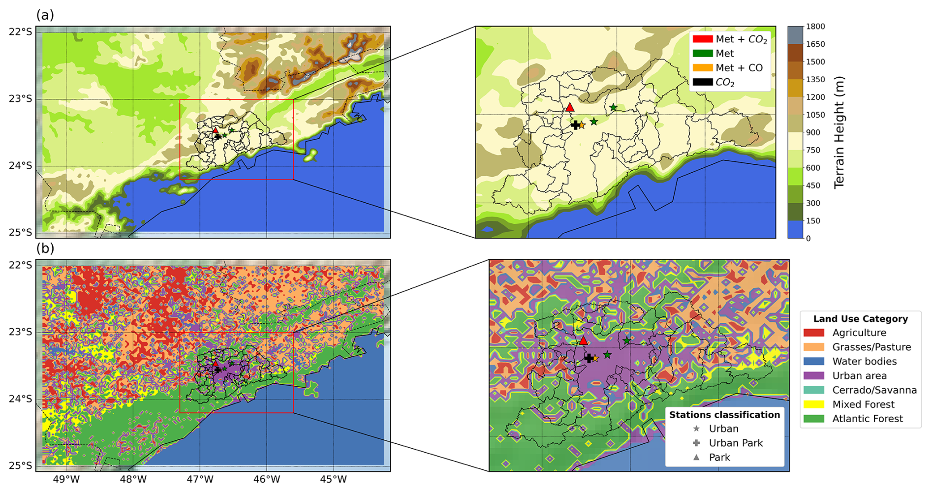
Figure 1 Panel (a) shows the terrain height and urban boundaries of the MASP region within the WRF-Chem model domain (D01). Station classifications are indicated using different symbols: Urban (gray star), Urban Park (gray cross), and Park (gray triangle). Panel (b) presents the land use category map for the same domain (D01), which was used by the VPRM model to calculate CO₂ fluxes. The colors of the station markers represent the type of measurements conducted at each location: red indicates stations measuring both meteorological variables (Met) and CO₂ concentrations, green indicates stations measuring only Met, dark yellow denotes stations measuring both Met and CO concentrations, and black indicates stations measuring only CO₂ concentrations. The IAG station is marked as a black cross, the PDJ station is a red triangle, the Pinheiros station is a yellow star, and Guarulhos and Parque D. Pedro II are green stars.

(Morrison et al., 2009)Iacono et al. (2008)Iacono et al. (2008)Hong et al. (2006)(Tewari et al., 2007)Crippa et al. (2021)(Ibarra-Espinosa et al., 2018)Mahadevan et al. (2008)

Table 1 WRF-Chem simulation design.

2 WRF-Chem

2.1 Model setup

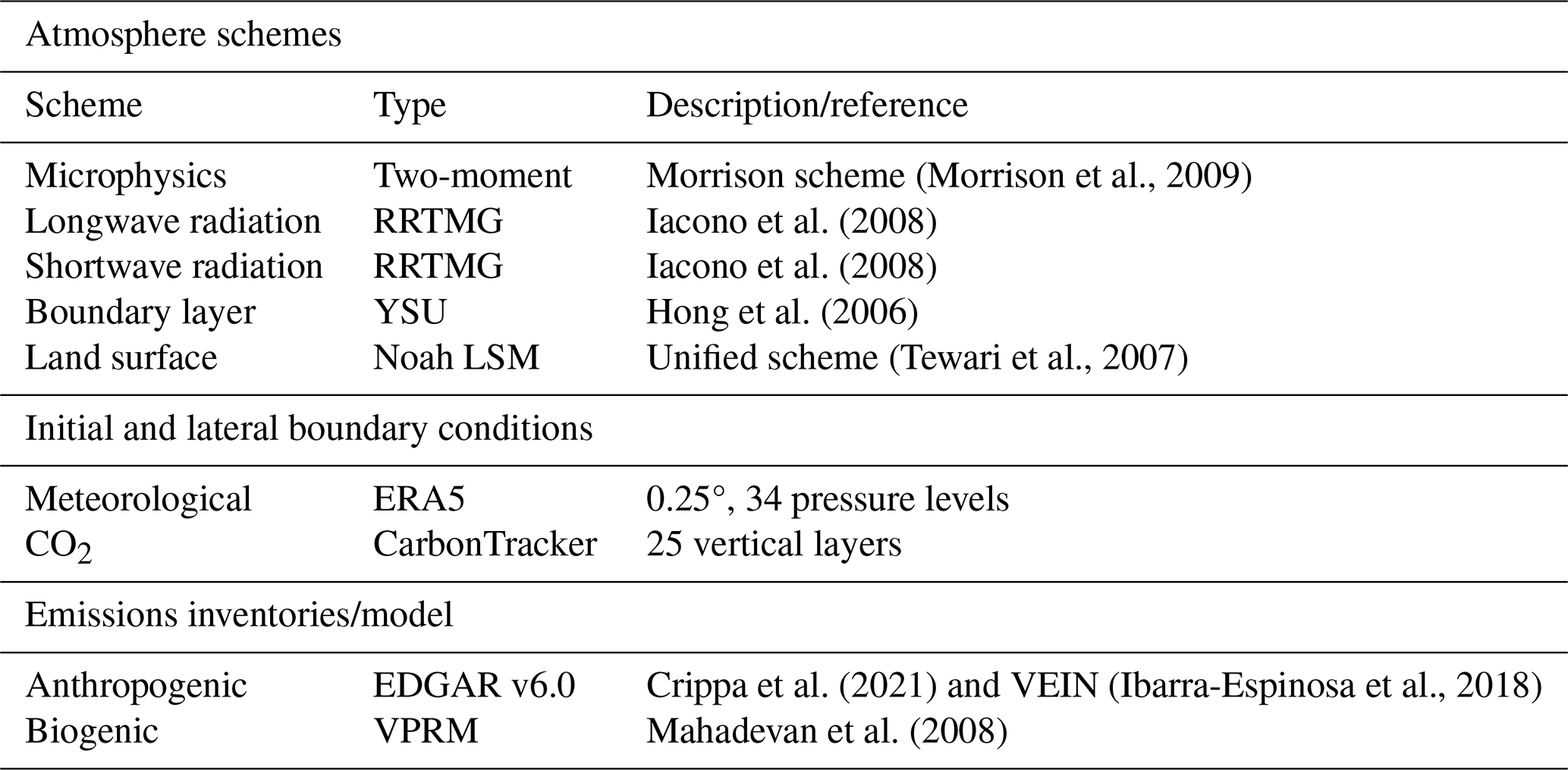
A set of high-resolution simulations of atmospheric Greenhouse Gas concentrations were performed with the WRF-Chem model version 4.0. The WRF-Chem was used to simulate the transport of the mole fraction of CO₂, and no chemical processes or reactions were used. The period simulated was from 1 February to 31 August 2019. This period was selected due to available data from monitoring stations from the METROCLIMA network for CO₂. The simulations were made for each month. For each run, the simulation was initiated 5 d before, and this period of 5 d was discarded as spin-up time. The single modeling domain was centered at 23.5° S and 46.3° W with a horizontal grid spacing of 3 km as shown in Fig. 1, projected on a Lambert plane and consists of 166 grid points in the west–east direction, 106 grid points in the north–south direction, and 34 vertical levels that extend from the surface up to 50 hPa (20 km), as used in previous studies for this same area (Andrade et al., 2015; Vara-Vela et al., 2016; Gavidia-Calderón et al., 2023; Benavente et al., 2023). The meteorological conditions used to drive the simulations were obtained from the European Centre for Medium-Range Weather Forecasts (ECMWF) ERA5 reanalysis dataset, with a horizontal resolution of 0.25°×0.25° and 6-hourly intervals (Hersbach, 2016). For CO₂, initial and boundary conditions were provided by CarbonTracker, which offers data at a horizontal resolution of 3° in longitude and 2° in latitude, with 25 vertical layers (http://carbontracker.noaa.gov, last access: 20 April 2024). This global dataset was interpolated to provide lateral boundary conditions for the simulations and ensure consistency with the WRF-Chem. The main physics and chemistry options used in this study are listed in Table 1.

2.1.1 Anthropogenic emissions

In the MASP, the vehicular fleet is the primary source of CO₂ emissions (CETESB, 2019). For this study, we employed the VEIN model, a tool designed to estimate emissions from mobile sources. VEIN accounts for both exhaust and evaporative emissions performs speciation, and includes functions to generate and spatially allocate emissions databases (Ibarra-Espinosa et al., 2018). The model enables the use of customized emission factors, which in this study were derived from experimental campaigns conducted in traffic tunnels within São Paulo (Nogueira et al., 2021). VEIN processes vehicle fleet age distributions, extrapolates hourly traffic data, and estimates emissions with high temporal and spatial resolution. For consistency with the WRF-Chem model domain, VEIN emissions were aggregated to a 3 km spatial resolution. Additionally, we included Fig. B1, which illustrates the spatial distribution of average daily CO₂ emissions for August 2019, the total monthly emissions from February to August, and the diurnal profile of vehicular CO₂ emissions as estimated by the VEIN model. Emissions from the industry, refinery, residential, and energy sectors were obtained from the EDGAR v6.0 GHG inventory for 2018 (Crippa et al., 2021). EDGAR provides global annual emissions at 0.1°×0.1° spatial resolution, which we regridded to 3 km using bilinear interpolation to match the WRF-Chem model domain. EDGAR does not provide hourly temporal profiles; these emissions were assumed constant over the day (Fig. B2). To evaluate the relative contribution of each sector to total emissions in the MASP, Fig. B3 presents the average daily CO₂ emissions in August 2019. Transport emissions represented the dominant share, accounting for 76.1 %, followed by industry (10.0 %), refinery (7.6 %), residential (3.8 %), and energy (2.5 %) sectors.

2.1.2 Biogenic fluxes

Biogenic CO₂ fluxes were simulated offline using the VPRM model (Mahadevan et al., 2008) and incorporated as flux input data in the WRF-Chem simulations. This model estimates net ecosystem exchange (NEE) by calculating the difference between gross ecosystem exchange (GEE) and ecosystem respiration (R), where negative fluxes indicate CO₂ absorption by ecosystems (Eq. 1).

$$\begin{array}{}\text{(1)}& \mathrm{NEE}=\mathrm{GEE}-R\end{array}$$

The meteorological variables 2 m air temperature (T_2 m) and downward shortwave radiation (PAR) from WRF model simulations were used to calculate the GEE (Eq. 2) and respiration (Eq. 3) fluxes. Additionally, factors such as the light use efficiency (λ), PAR saturation (PAR₀), and the Enhanced Vegetation Index (EVI), which refer to as the fraction of shortwave radiation absorbed by leaves, were used to calculate GEE. The temperature sensitivity of the photosynthesis parameter (Tscale) and the effects of leaf age on canopy photosynthesis parameter (Pscale) were both calculated as functions of the land surface water index (LSWI) to identify the green-up (leaf expansion) and senescence phases (Mahadevan et al., 2008). These vegetation indices were derived from Moderate Resolution Imaging Spectroradiometer (MODIS) reflectance data from MOD09A1 version 6 (Vermote, 2021).

$$\begin{array}{}\text{(2)}& \mathrm{GEE}=\mathit{\lambda }\times T_{\mathrm{scale}}\times P_{\mathrm{scale}}\times W_{\mathrm{scale}}\times \mathrm{EVI}\times {\displaystyle \frac{\mathrm{1}}{\mathrm{1}+\frac{\mathrm{PAR}}{{\mathrm{PAR}}_{\mathrm{0}}}}}\times \mathrm{PAR}\end{array}$$

Respiratory fluxes (R) were estimated using a linear model based on air temperature and two parameters that represent the linear sensitivity of respiration to air temperature (α) and the baseline respiration (β), as defined in Mahadevan et al. (2008).

$$\begin{array}{}\text{(3)}& R=\mathit{\alpha }\times T_{\mathrm{2}\mathrm{m}}+\mathit{\beta }\end{array}$$

The land cover data used by the VPRM were derived from the MapBiomas data (Souza et al., 2020). The VPRM parameters (λ, PAR₀, α, β) were optimized against flux tower NEE for the main land cover type over the study domain described in Sect. 2.2.2.

2.1.3 Meteorological data

Meteorological data from the São Paulo State Environmental Protection Agency (CETESB) air quality network were used to evaluate the model's performance in simulating meteorological fields. CETESB manages automatic and manual air quality stations over São Paulo state. These stations provide hourly information on meteorological and pollutant parameters, such as air temperature, wind speed, and wind direction (Table 2), as well as the concentration of air pollutants. Monitoring follows instrumentation standards and directives from the Environmental Protection Agency (US EPA) and the World Health Organization (WHO), respectively, for air pollutants and from the World Meteorological Organization (WMO) for meteorological variables (CETESB, 2019). The air quality and meteorological data are continuously published on the Qualar website (https://qualar.cetesb.sp.gov.br/qualar/, last access: 10 July 2024). This study used data from four stations located in the MASP (Fig. 1): Parque D. Pedro II, PDJ, Guarulhos, and Pinheiros. Table 2 provides the location of the sites, the classification type of the stations, the observed variables, and the data source.

Table 2 Location of the sites used for the model evaluation of the meteorological drivers, together with a list of the meteorological variables included in the analysis.

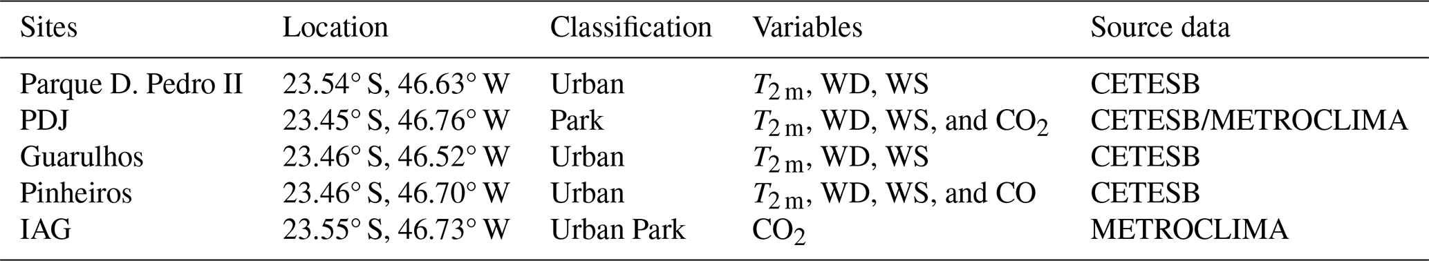
Note: air temperature at 2 m (T_2 m), wind speed (WS), and wind direction (WD).

2.2 CO₂ observational data

2.2.1 Ground-based observations

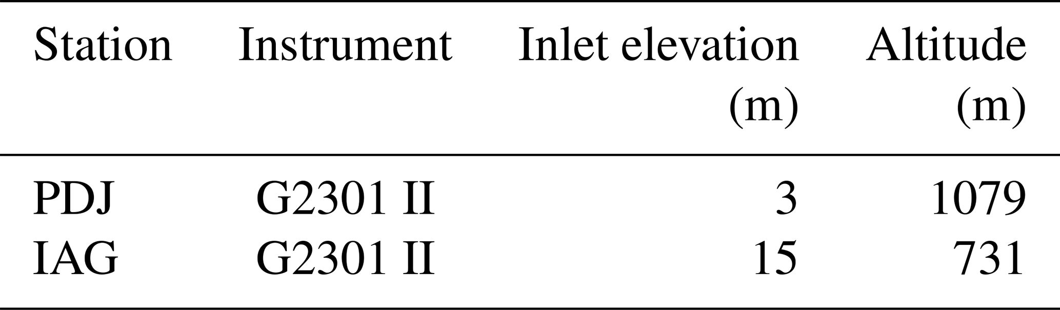
We assessed near-surface model performance using CO₂ observations from the METROCLIMA network in São Paulo (see Table 3 and Fig. 1), the first conventional in situ greenhouse gas measurement network established in South America (http://www.metroclima.iag.usp.br/, last access: 12 July 2024). The network comprises four continuously operating monitoring stations, all located within the MASP and equipped with cavity ring-down spectroscopy instruments (Picarro) that measure the concentrations of CO₂ following the directives from WMO. The monitoring stations are located at various locations within MASP: in a vegetated area at the extreme west (Pico do Jaraguá, PDJ); in a suburban area in the center west, inside the campus of the University of São Paulo (IAG); at the top of a 100 m building (ICESP); and in an urban area in the east zone characterized by heavy traffic in the neighborhood (UNICID). However, we only used data from the IAG and PDJ sites, which are 13 km apart, as these were the only two stations monitoring CO₂ during the selected study period, prior to the Covid-19 pandemic (Souto et al., 2023).

Table 3 Description of the METROCLIMA monitoring stations utilized in this study.

2.2.2 CO₂ flux data and VPRM optimization

In this study, the VPRM model computed the biosphere fluxes for five different plant functional types (PFTs), representing different vegetation land covers, and for that required a set of four model parameters for each vegetation class, dependent on the region of interest. Ideally, these parameters are optimized using a network of eddy flux towers for each PFT over the domain. The VPRM parameters were optimized for only three PFTs corresponding to the three ecosystems observed by eddy-covariance flux towers. However, these three PFTs represent almost 60% of land covers over the domain (i.e., sugarcane – 23.86 %, Atlantic Forest – 34.86 %, and Cerrado – 0.91 %). We used a set of parameters optimized by Botía et al. (2022) for the remaining PFTs, such as grasses and mixed forest, based on measurements from sites in the Amazon region in Brazil, deployed in the context of the Large Scale Biosphere-Atmosphere Experiment (LBA-ECO) (Botía et al., 2022). The methodology for optimizing the VPRM parameters for the Atlantic Forest used data from the Serra do Mar State Park in São Paulo state, Brazil (23°17^′ S, 45°03^′ W, at 900 m altitude), for the period from January 2015 to December 2015 (Freitas, 2012). For Cerrado, we used observed data from Pé Gigante, in São Paulo, Brazil (21°36^′ S, 47°34^′ W, at 660 m), from January 2015 to January 2017 (Rocha et al., 2002). For sugarcane we used data from the municipality of Pirassununga, in São Paulo state, Brazil (21°57^′ S, 47°20^′ W, at 655 m altitude), for the period from November 2016 to August 2017 (Cabral et al., 2020). The VPRM parameters were optimized separately for each PFT using half-hourly observed fluxes from the flux towers over the entire observation periods. We optimized the parameters for the GEE and R simultaneously, and for the default VPRM parameters we used non-linear least squares minimization between the modeled NEE and the flux tower estimation of the observed NEE. In the optimization, the VPRM model is driven by the meteorological measurements of the sites and their specific land covers. The vegetation indices (EVI and LSWI) were derived from the product MOD09A1 of MODIS at 500 m resolution and 8-daily frequency using Google Earth Engine.

2.2.3 XCO₂ satellite observations

Satellite-based XCO₂ observations were utilized in addition to surface CO₂ measurements over the study domain. OCO-2, NASA's inaugural Earth remote sensing satellite dedicated to atmospheric CO₂ observations, was launched in 2014 (Crisp, 2015). Operating on a solar synchronous orbit, OCO-2 conducts global measurements of CO₂ absorption and emission at 13:30 LST (local solar time). The OCO-2 observation data utilized were ACOS L2 Lite with oco2-lite_fle_prefilter_b9, which were converted from Level 1 radiance to Level 2 data using the ACOS retrieval algorithm developed by O'Dell et al. (2012). Data quality assessment for OCO-2 observations can be performed using the xco2_quality_flag and warn_level parameters, as detailed in the OCO-2 Data Product User's Guide (Osterman et al., 2018). In this study, we considered only OCO-2 data with a “0” xco2_quality_flag value that indicates good quality. Initially, simulated CO₂ concentrations were interpolated to match the latitude, longitude, horizontal resolution, and vertical levels of OCO-2 data. Additionally, to ensure consistency in the comparison, the simulated data were selected to correspond as closely as possible to the OCO-2 overpass time (13:30 LST) over the study region. Due to the difference in data types and units between the simulated CO₂ concentrations and observed XCO₂ from satellites, a conversion was necessary prior to comparison. Consequently, CO₂ concentrations simulated at each pressure level in the WRF-Chem were transformed into XCO₂ concentrations following the methods by Connor et al. (2008) and O'Dell et al. (2012), as follows:

$$\begin{array}{}\text{(4)}& X{{\mathrm{CO}}_{\mathrm{2}}}^{\mathrm{model}}=X{\mathrm{CO}}_{\mathrm{2}\mathrm{a}}+\sum _i{w}_i^T{A}_i{\left({{\mathrm{CO}}_{\mathrm{2}}}^{\mathrm{interp}}-{\mathrm{CO}}_{\mathrm{2}\mathrm{a}}\right)}_i,\end{array}$$

where XCO_2a is a priori XCO₂, $w_i^T$ is the pressure weighting function, A_i is the column averaging kernel, CO${}_{\mathrm{2}}^{\mathrm{interp}}$ is the interpolated simulated CO₂ concentrations of WRF-Chem, and CO_2a is a priori CO₂.

2.3 Evaluation metrics

Several statistical metrics are available for assessing the effectiveness of atmospheric models. These include mean bias error (bias, Eq. A1), indicating the average difference between the simulation and the observation; root-mean-square error (RMSE, Eq. A2), which quantifies the square root of the average squared deviation between simulation and observation; and the correlation coefficient (R², Eq. A3), representing the degree and direction of the linear connection between the simulation and the observation. To evaluate the model performance, we calculated the bias, RMSE, and R², with the corresponding equations provided in Appendix A.

3 Results

Hourly simulations were conducted from 1 February to 31 August 2019, with each month simulation including a 5 d spin-up period. In the following sections, the performance of meteorological drivers will first be presented, followed by the terrestrial surface CO₂ fluxes and atmospheric CO₂ concentrations from the IAG and PDJ stations. These measurements were used to evaluate the model performances and to assess the local impacts of the main CO₂ sources and sinks on atmospheric CO₂ concentrations.

3.1 Model performance for meteorological drivers

The assessment of the meteorological model performances is essential for accurately simulating greenhouse gas concentrations. In this study, the model represented the temporal variability and trends of 2 m temperature (T_2 m), 10 m wind speed (WS), and direction (WD) throughout the simulation period, as illustrated in Fig. 2 and in Appendix B (see Figs. B4, B5, and B6). The WRF-Chem model effectively captured significant changes in the observed variables, although it failed to accurately represent the maximum and minimum peaks, particularly for wind speed. The simulated 2 m temperature tended to overestimate values at specific sites, such as Parque D. Pedro II (bias = 0.5 °C), Guarulhos (bias = 0.1 °C) (see Figs. B4a and B5a), and PDJ (bias = 0.7 °C) (see Fig. 2a). However, at the Pinheiros station, the simulated surface temperature was underestimated (bias = −0.7 °C) (Fig. B6a).

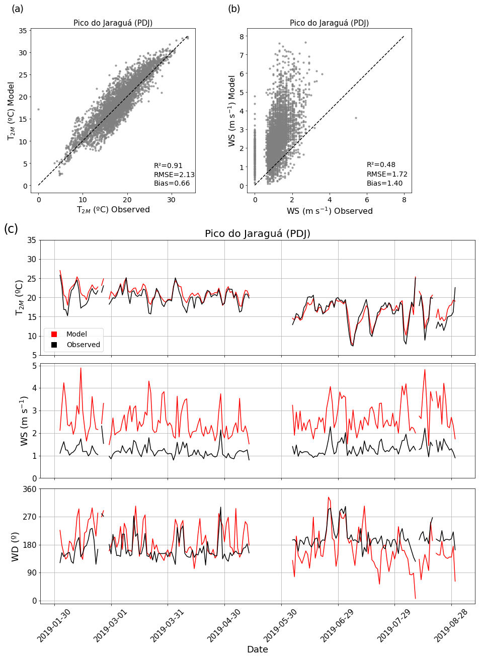
Figure 2 Panels (a) and (b) show scatter plots comparing model outputs and observations at the PDJ station for hourly values of 2 m air temperature (T_2 m) and 10 m wind speed (WS), respectively. Panel (c) presents the daily averages from February to August 2019 for 2 m air temperature (T_2 m), 10 m wind speed (WS), and wind direction (WD). The black line represents observational data, while the red line indicates model simulations.

In terms of biases, the model overestimated the wind speed at all sites (bias < 1.5 m s⁻¹), with PDJ exhibiting the highest mean bias (1.4 m s⁻¹). This overestimation could be attributed to the model's misrepresentation of land use, leading to elevated wind speeds in areas classified as urban rather than vegetated. Notably, numerical models tend to lack sensitivity in simulating very low-velocity speeds due to imperfections in land surface processes and the model's ability to accurately resolve topographical features (Shimada et al., 2011; Zhang et al., 2009; Vara-Vela et al., 2018, 2021). The model's wind directions showed sufficient sensitivity, aligning accurately with observed values. Both the model and observations indicated that prevailing winds were predominantly from the southeast. In summary, the WRF model showed proficiency in reproducing atmospheric conditions in the study area, particularly concerning air temperature and wind direction, with similar performances to previous studies (Feng et al., 2016; Deng et al., 2017).

3.2 The VPRM model: evaluation with flux tower data

The optimization results are shown in Table 4. Substituting alpha and beta back into the respiration equation led to a better model representation of NEE compared to NEE values simulated with default parameters (Mahadevan et al., 2008) for the main PFT across the domain.

Botía et al. (2022)

Table 4 Default (Mahadevan et al., 2008) and optimized VPRM parameters (highlighted) for Atlantic Forest, Cerrado, and sugarcane and for mixed forest and grasses from Botía et al. (2022).

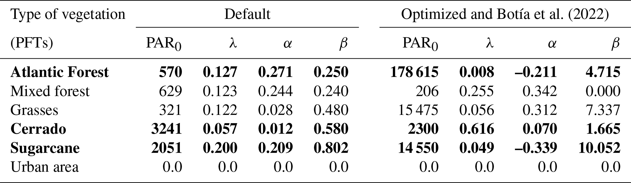
The optimized VPRM parameters for the Atlantic Forest exhibited the greatest discrepancies compared to other vegetation classes. The geomorphological characteristics of the Atlantic Forest differ from those of the evergreen forest studied by (Mahadevan et al., 2008), where the default parameters (VPRM_default, represented by the red curve in Fig. 3) were used. The optimized VPRM parameters (VPRM_optimized, shown as the green curve in Fig. 3) more accurately captured the seasonal cycle in the daily average NEE for the three PFTs optimized in this study. The model was particularly successful in capturing the seasonal profile for the agricultural ecosystem, which can be attributed to the more pronounced seasonal transitions of sugarcane (as indicated by the EVI), even though the low-resolution satellite indices do not fully capture the onset of the growing season. However, this allowed the model to better represent the GEE equation for this ecosystem. For the Cerrado, the model smoothed the NEE peaks, and the GEE and respiration equations were also smoothed with the optimization. Optimizing the VPRM parameters improved the representation of the growing season, especially for the Atlantic Forest and sugarcane, while using optimized or default parameters for the Cerrado resulted in similar NEE simulation.

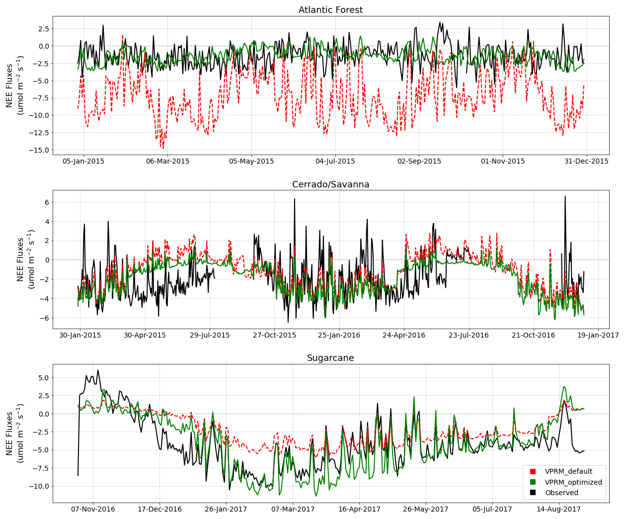
Figure 3 Daily variability of NEE fluxes (µmol m⁻² s⁻¹) from the flux tower (black line), compared with NEE fluxes simulated by the VPRM model using default (red line) and optimized (green line) parameters for the Atlantic Forest, Cerrado/savanna, and sugarcane.

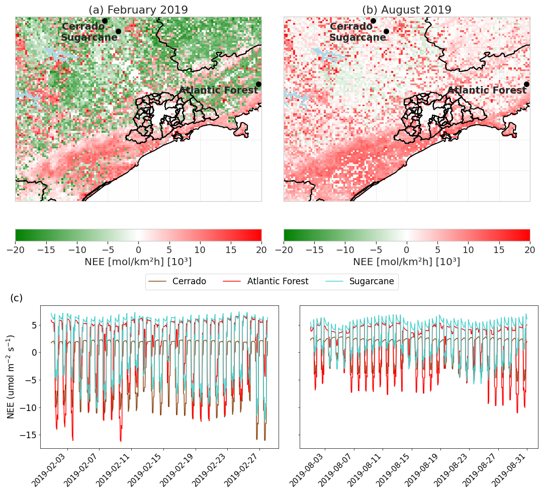
Figure 4 The top panels show the monthly mean of net ecosystem exchange (NEE) (mol km⁻² h⁻¹) for February (a) and August 2019 (b). The bottom panel (c) presents the hourly variability of NEE (µmol m⁻² s⁻¹) for the same months (February and August) at three different PFTs: Atlantic Forest, Cerrado/savanna, and sugarcane.

The top panels in Fig. 4 show the monthly net CO₂ flux simulated by the VPRM model for 2019. February represents a summer month, while August represents a winter month. The bottom panel shows the monthly hourly net CO₂ flux simulated at the three flux tower sites used to optimize the VPRM model parameters. In February, negative NEE values are found in the northern part of the MASP, while the southern part exhibits positive NEE fluxes in the coastal region. During the summer, ecosystem productivity is expected to peak across all land cover classes, typically resulting in negative NEE. This behavior was clearly observed in February (Fig. 4a) for Cerrado, sugarcane, and pasture areas. In contrast, the Atlantic Forest in the southwestern portion of the domain exhibited positive NEE values, an unexpected pattern for a summer month. This may be linked to a combination of structural and anthropogenic factors, as well as limitations of the model itself. The Atlantic Forest is marked by structural heterogeneity, extreme biodiversity, and high fragmentation, which can lead to significant local variation in CO₂ fluxes. In addition, the SEEG (2021) report highlights a progressive decline in the biome's carbon sink function. Model limitations also likely contribute to these discrepancies, particularly simplifications in VPRM's equations of respiration and phenology, which may not fully capture the complex dynamics of ecosystems like the Atlantic Forest (Rezende et al., 2018; Segura-Barrero et al., 2025).

In August, the cold and dry conditions, due to reduced solar radiation and a lower leaf area index, resulted in positive fluxes across most of the domain and low negative fluxes in only a few areas (Fig. 4b). The highest positive NEE values are found in the southern coastal region. Generally, larger areas with negative CO₂ fluxes are observed in February compared to August for the same dominant land cover classes. This indicates greater CO₂ absorption by agriculture in February compared to forested regions. Conversely, in August, CO₂ fluxes are predominantly lower and negative across most of the domain, with higher positive values in the coastal area, especially in the south. Overall, the domain acts as a net CO₂ sink during summer, while vegetation becomes a CO₂ source in winter, except for the Atlantic Forest in the southern part of the study area. The bottom panel also shows simulated fluxes for the same flux tower sites, with negative net fluxes in February, particularly in the Atlantic Forest, sugarcane, and Cerrado. This underscores the reduction in negative fluxes during winter, as seen in the August data for all three vegetation types. Unfortunately, observed data from these flux towers for this period were not available for statistical model evaluation. However, Fig. 4 illustrates the significant influence of climatic drivers on reduced flux trends, consistent with findings by Raju et al. (2023) for a tropical region. Note that the respiration equation in Mahadevan et al. (2008) is a simple linear function of temperature and does not account for seasonal or spatial variability in biomass and litter inputs to soil carbon pools (Gourdji et al., 2022), which is particularly relevant for forest ecosystems like the Atlantic Forest.

3.3 Seasonal variations in observed and modeled CO₂ mixing ratios

Figure 5 and Table 5 depict the monthly mean, standard deviation, bias, and RMSE of CO₂ concentrations at two sites in the MASP. In 2019, the IAG station recorded CO₂ values ranging from 406 to 464 ppm. The seasonal variation peaked during winter (June to August, 437.3±32.2 ppm), followed by autumn (March to May, 433.0±26.0 ppm), with the lowest values observed in summer (February, 432.7±24.6 ppm). This variation in CO₂ levels is primarily influenced by the geographical location of the observation site, meteorological conditions such as wind speed and atmospheric stability, and seasonal patterns of photosynthesis and vehicular traffic (see Fig. B1). The maximum and minimum monthly CO₂ concentrations at IAG were recorded in June (442.5±32.8 ppm), during the winter season, and March (430.2±24.5 ppm), during the autumn season, respectively. During this month, the MASP experiences changes in synoptic circulation and atmospheric moisture that typically reduce atmospheric stability and increase the dispersion of various gases and particles (Chiquetto et al., 2024). Meanwhile, at the PDJ station, CO₂ levels ranged from 414 to 417 ppm. The seasonal variation peaked during autumn (416.8±9.5 ppm), closely followed by summer (416.0±10.3 ppm), with the lowest values observed in winter (414.6±7.4 ppm). The maximum monthly CO₂ mean at PDJ was identified in May (417.3±9.1 ppm), corresponding to the autumn season, while the minimum was recorded in July (414.0±6.3 ppm), during the winter season. Monthly values at PDJ exhibited less variability and a smaller standard deviation compared to the IAG site. This result was expected, considering that the IAG site is significantly impacted by vehicular traffic in its vicinity. In contrast, PDJ is located at a higher elevation in a more vegetated area, with less influence from local anthropogenic sources. Additionally, lower CO₂ concentrations were expected at PDJ during the summer due to the stronger vegetation signal compared to the IAG site. However, PDJ actually shows peak CO₂ levels in summer and the lowest values in winter, indicating that additional ecological and ecosystem variables need to be considered for a better understanding of this location.

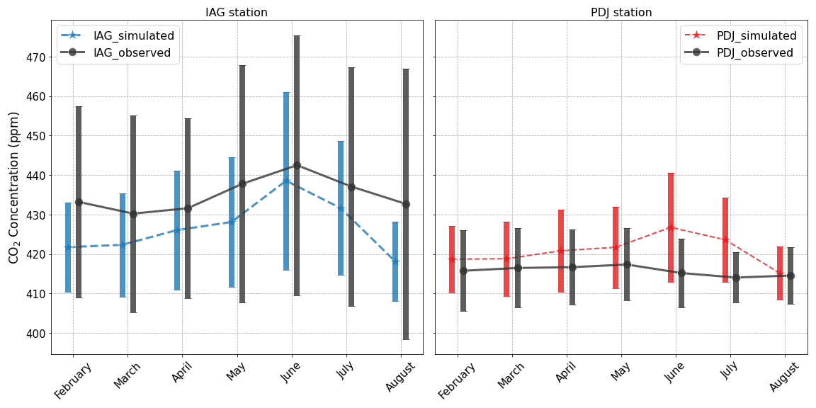
Figure 5 CO₂ concentration seasonality observed and simulated at IAG and PDJ stations in 2019. Error bars represent the monthly standard deviation.

Table 5 Seasonality means and standard deviation of CO₂ concentrations for IAG and Pico do Jaraguá (PDJ) stations.

The simulated CO₂ concentrations for the IAG station ranged from 410 to 437 ppm, with a seasonal variation peaking in winter (429.4±19.2 ppm), followed by autumn (425.2±15.1 ppm), and the lowest values occurring in summer (422.3±12.3 ppm), mirroring the observed data. Notably, the highest and lowest monthly CO₂ concentrations at IAG were identified in June (438.7±22.5 ppm) and February (418.1±10.0 ppm), respectively. Although the maximum monthly value from the model coincided with the observed data, the month with the minimum concentration was February, which may be attributed to gaps in measurement, which were not considered when calculating the mean, thereby influencing the observed monthly mean. The CO₂ concentrations at PDJ ranged from 415 to 426 ppm, with seasonal variation peaking in winter (421.8±11.8 ppm), followed by autumn (420.4±10.1 ppm), and the lowest values occurring in summer (419.0±8.8 ppm). The model data profile for PDJ more closely resembles the simulated IAG profile than the PDJ station's observed profile, which likely stems from model limitations, including grid resolution and insufficient representation of localized characteristics at different sites. However, negative biases were observed for all seasonal periods at IAG, indicating an underestimation of CO₂ concentrations and higher RMSE compared to the statistics for the PDJ station. The PDJ station exhibited low positive biases and smaller standard deviations between the model and observations. Its higher elevation and dense vegetation cover simplify the representation of seasonal trends, reducing the influence of urban emissions and resulting in lower CO₂ concentrations at this site (see Fig. B7).

3.3.1 Distribution of surface CO₂ concentrations

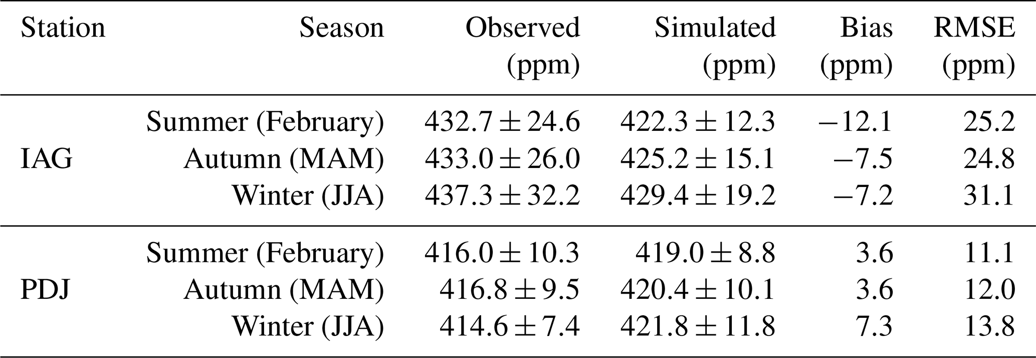
In addition to the simulations conducted for the period from February to August 2019, using the same configurations and input data, we performed simulations involving variable emission scenarios for the summer (February) and winter (August) seasons. The aim was to comprehensively understand the dynamics of CO₂ concentration in the metropolitan region and surrounding areas during these distinct seasonal periods. Figure 6 shows the monthly average spatial distributions of simulated CO₂ concentrations under four conditions: (a) background without emissions, considering only boundary and initial conditions (BCK); (b) considering both anthropogenic emissions and biogenic fluxes (see Table 1) (ALL); (c) considering biogenic fluxes only (BIO); and (d) considering anthropogenic emissions (energy, industry, residential, refinery, and vehicular sectors) only (ANT).

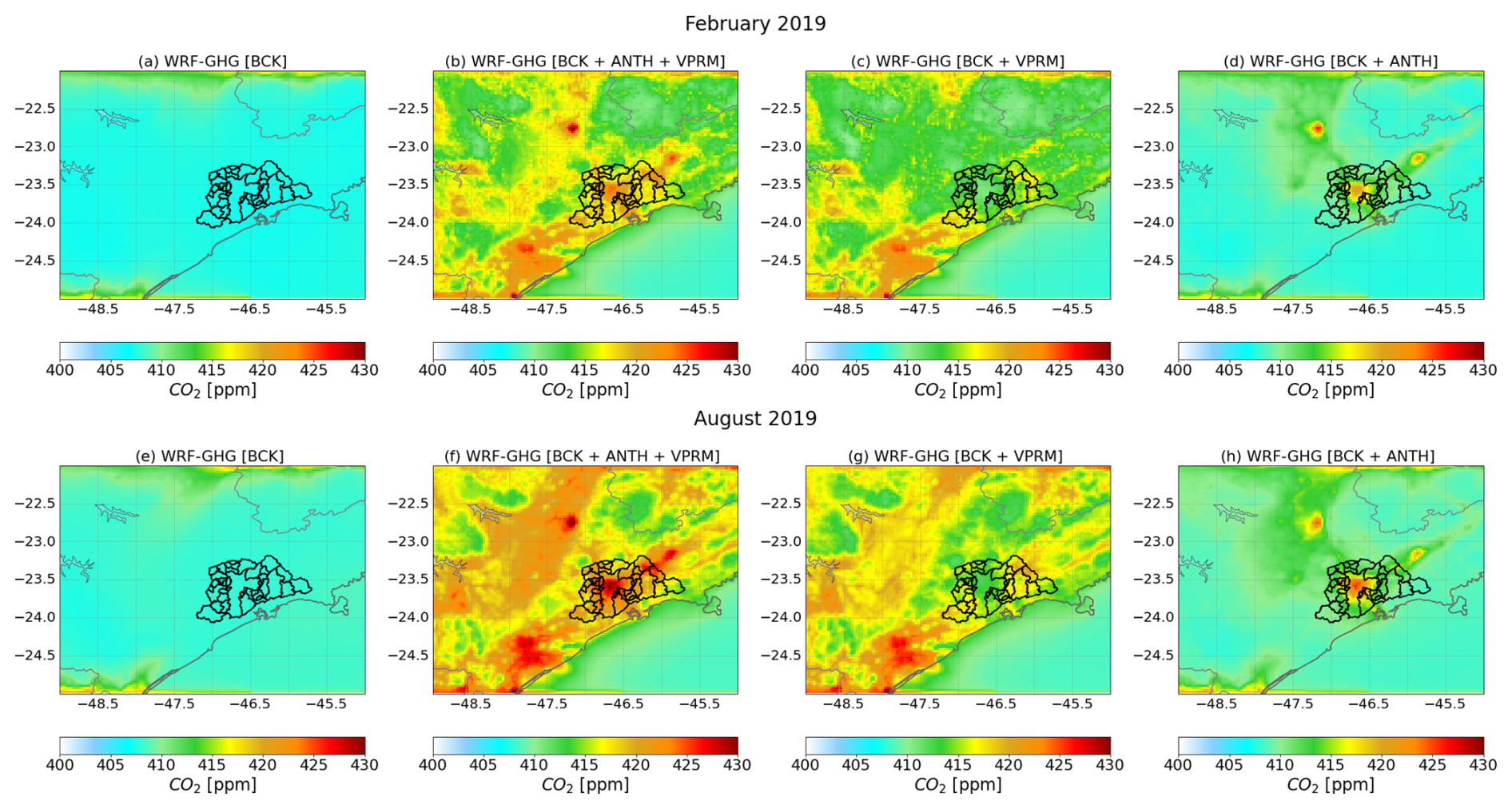
Figure 6 Atmospheric CO₂ concentrations under different emission scenarios (refer to the text). The panels in the first row represent the monthly mean concentration for February (a–d), while the panels in the second row represent the monthly mean concentration for the August period (e–h). Panels (a) and (e) represent the background scenario. Panels (b) and (f) represent the simulation of the total (background, anthropogenic, and biogenic) emission scenario, panels (c) and (g) represent the simulation of only the background and biogenic scenario, and (d) and (h) represent the simulation of only the background and anthropogenic scenario.

Figure 6a shows that the simulated background CO₂ concentration in February ranged around 408 ppm across most of the domain. For biogenic simulations (Fig. 6c), we observed an average increase of 14 ppm across the domain compared to the previous simulation. The increase, however, was only 6 ppm in downtown MASP. Although the VPRM model did not explicitly calculate CO₂ fluxes in urban areas due to limited vegetation coverage, the transport of biogenic signals from the surrounding vegetated regions into the urban area is evident. The southwest region of the domain, characterized by the Atlantic Forest, exhibits the highest CO₂ concentrations in this scenario, ranging from 420 to 424 ppm. This dense vegetation region and higher ecosystem respiration contribute to elevated CO₂ levels, underscoring the influence of biogenic sources on regional concentration patterns. This region has altitudes lower than 200 m, and the CO₂ released to the atmosphere by the vegetation is trapped due to the Serra do Mar, with altitudes higher than 500 m. The Atlantic Forest present on the northern coast, on the other hand, is concentrated on the plateau of Serra do Mar, and thus the CO₂ released is better dispersed to other areas. The simulation with anthropogenic emissions (Fig. 6d) stands out with elevated CO₂ concentrations over the center of the city of São Paulo, characterized by high vehicle emissions, as well as over other two urban areas in the north and northeast of MASP. The monthly mean CO₂ concentration in these two urban areas was roughly 420 ppm, attributed to emissions from refineries represented by the EDGAR datasets as well as vehicles. Figure 6b shows the simulated CO₂ concentration considering both vegetation fluxes and anthropogenic emissions. As expected, this simulation combines both contributions, resulting in high CO₂ concentrations over urban areas and along the coastal region. For August, it can be observed that the background concentrations (Fig. 6e) were slightly higher around MASP. Additionally, the monthly mean CO₂ concentration for the scenario in August with only biogenic sources was 8 ppm higher than that in February, which can be explained by the lower photosynthetic rates in this period, as observed in Fig. 4. The Atlantic Forest in the coastal region exhibits more positive CO₂ fluxes and lower photosynthetic activities, characterized by lower amounts of rainfall in the region that contribute to this reduced photosynthetic production by vegetation. The simulation with only anthropogenic emissions (Fig. 6h) shows higher CO₂ concentrations compared to those in February. This increase in CO₂ levels in August is attributed to a lower planetary boundary layer (PBL) height. However, it is important to point out that the EDGAR anthropogenic emission inventory generally overestimates the emissions around local anthropogenic sources (e.g., urban areas) (Seo et al., 2024). The higher simulated CO₂ concentration for August compared to February, in the scenario with both biogenic and anthropogenic sources, is largely dependent on factors such as atmospheric stability and meteorological conditions. Atmospheric stability, along with meteorological variables such as humidity, solar radiation, and temperature, plays a crucial role in determining biogenic CO₂ concentrations. In addition, under stable atmospheric conditions, such as those often observed during winter periods, CO₂ concentrations tend to accumulate near the surface, resulting in higher concentrations, especially in urban areas. Therefore, the comparative analysis between the simulations of CO₂ concentrations during summer and winter periods highlights the importance of accurately representing not only anthropogenic emissions, but also biogenic fluxes from vegetation.

Figure 7 Daily mean CO₂ concentrations simulated and observed for the IAG site in February 2019 (a), for the PDJ site in February (c), for the IAG site in August (e), and for the PDJ site in August (g). The daily mean CO₂ concentrations simulated under the BCK (background), VPRM (biogenic), and ANTH (anthropogenic) scenarios for the IAG site during February (b), for the PDJ site in February (d), for the IAG site during August (f), and for the PDJ site in August (h).

3.3.2 Evaluation of sources contribution

In Fig. 7, we applied a data selection scheme to all time series to minimize the effects of local contributions and increase the spatial representativeness of each record; it consists of retaining daytime (09:00–17:00 LT, local time) data, when the air is well mixed, providing a large spatial representativeness with minimum influence from local sources (Gerbig et al., 2008; Ramonet et al., 2020). Figure 7 shows the comparison of the daily daytime average CO₂ concentrations simulated by the model for February and August 2019, considering both biogenic and anthropogenic sources (see Fig. 6b and f) at both IAG and PDJ sites. The left panels (Fig. 7a, c, e, and g) depict the simulated CO₂ concentration considering both anthropogenic and biogenic sources (all_sources, in gray), alongside observed concentrations (observed, in purple) for both sites. Conversely, the right panels (Fig. 7b, d, f, and h) display the different simulations considering anthropogenic and biogenic sources separately from the daily concentration. In Fig. 7a, which represents only one summer month with available observational data (February 2019), the model generally underestimated CO₂ concentrations. The observed average was 424.0 ppm, while the simulated average was 416.0 ppm – an underestimation of approximately 8 ppm. This difference may be partially attributed to the presence of data gaps in the observational data for this site, as only available values were considered when calculating the monthly mean. For the anthropogenic sources the simulation is aligned with the expectations that the emission is dominated by vehicular emissions around this vicinity (Fig. 7b). However, on 23, 24, and 25 February there was a distinct peak in the observed CO₂ concentrations. This spike is absent in both the all-source and anthropogenic simulations, suggesting that other localized or transient activities, not accounted for in the emissions inventory, may have contributed. This discrepancy likely arises because the inventories assume identical emissions for all days with only hourly variations. As a result, specific events or activities that occur on these particular days are not captured in the simulations. Furthermore, on 2 and 22 February, observed CO₂ peaks were captured by the model with similar magnitude only when both anthropogenic and biogenic emissions were included.

At the PDJ site, the mean observed and simulated CO₂ concentration in February was 414 ppm. The model captures the overall trend and major peaks of CO₂ variability during this period, with biogenic contributions more pronounced at PDJ compared to the IAG site (Fig. 7d). This higher biogenic influence at PDJ is attributed to its location in a vegetated area and localized at a higher altitude than IAG, relatively isolated from vehicular emissions and other anthropogenic sources typical of urban environments, as previously discussed.

In August, characterized by a drier, more stable boundary layer and lower wind speed, observed data for IAG showed an average of 426 ppm (Fig. 7e), while the model showed a monthly average of 413 ppm, resulting in a discrepancy of 13 ppm, i.e., a higher difference compared to February. In terms of the contributions of the sources (Fig. 7f), simulations showed similar daily patterns, with a few days where CO₂ contributions from biogenic fluxes exceeded those from anthropogenic sources. In contrast, for PDJ (Fig. 7g), both the observed and simulated monthly average concentrations were 412 ppm. While the model slightly underestimated some days in the month and overestimated others, it generally captured the observed variability. Regarding the source contributions, the model simulation aligned with the observed temporal profile, displaying a more pronounced biogenic signal than at the IAG site, which further emphasizes the significant role of vegetation as a source of CO₂ emissions at this location (Fig. 7h). Before late August, observed values tended to be higher than the simulations, whereas in the final days of the month, the model overestimated CO₂ concentrations. This overestimation is associated with an increase in background concentrations – a pattern also observed at the IAG site during the same period.

The bias and RMSE for each simulation at the IAG and PDJ sites for February and August 2019 are illustrated (see Fig. B8). At IAG, the average bias ranged from −14.31 to −9.17 ppm, while at PDJ it ranged from −3.54 to −0.96 ppm. RMSE values were consistently higher at IAG, exceeding 20 ppm in most scenarios, while PDJ showed lower errors, generally below 12 ppm.

Considering that CO serves as a vehicular tracer, we analyzed CO concentrations at the Pinheiros site using data from the CETESB network (see Fig. 1 and Table 1) to compare with CO₂ concentration profiles at the IAG site for February to August 2019, located less than 3 km away from the Pinheiros site. The hourly correlation between observed CO₂ concentrations at the IAG site and observed CO concentrations at Pinheiros was determined, along with the correlation between simulated CO₂ concentrations for IAG and observed CO concentrations. In Fig. 8, both bar graphs of the hourly correlation between CO₂ and CO concentrations show values above 0.5 for observed CO₂ and above 0.25 for simulated CO₂ during the early hours of the day (until 10 h) and again in the evening (after 19 h). At midday, this correlation decreases and even turns negative for the simulated CO₂ vs. CO graph, suggesting the influence of the photosynthesis process on CO₂ concentrations, which is also evident in the observed data. The similarity between the trend lines of the hourly correlation profiles for observed CO₂ vs. CO and simulated CO₂ vs. CO is evident.

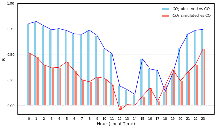
Figure 8 Hourly correlation between CO₂ concentrations observed at the IAG site and CO concentrations observed at the Pinheiros site (blue bars) and between simulated CO₂ concentrations at the IAG site and observed CO concentrations at the Pinheiros site (orange bars) for the period from February to August 2019.

In addition to the correlation between gases, Fig. 9 indicates that both the modeled and observed CO₂ profiles suggest that a significant portion of the CO₂ concentrations at the IAG site originates from vehicular sources, as carbon monoxide is a trace gas associated with traffic emissions (Nogueira et al., 2021). Peaks in the CO₂ time series at IAG are observed at the beginning, where the model fails to capture the magnitude of these concentrations. These peaks also appear in the observed CO profile at the beginning of the month, confirming that a large part of the CO₂ concentrations at IAG comes from vehicular sources, particularly on days with high concentrations, which are also reflected in the CO profile. However, the model struggles to simulate these high CO₂ concentrations since it assumes that emissions follow the same diurnal variation every day of the month. Additionally, a distinct increase in CO concentrations without a corresponding rise in CO₂ was observed between 18 and 21 August and 27 and 28 August, which coincided with the long-range transport of smoke plumes from Amazon forest fires to São Paulo (Bencherif et al., 2020). While biomass burning emits both CO and CO₂, their atmospheric transport and dispersion differ significantly. CO is more prevalent in incomplete combustion and tends to be transported at altitudes that favor long-range dispersion, whereas CO₂ concentrations are more influenced by local emissions and atmospheric mixing (Gatti et al., 2010). These transport dynamics, combined with the long distance of the event's origin, likely explain why the CO peak was detected at Pinheiros but not accompanied by a significant CO₂ enhancement at the IAG site.

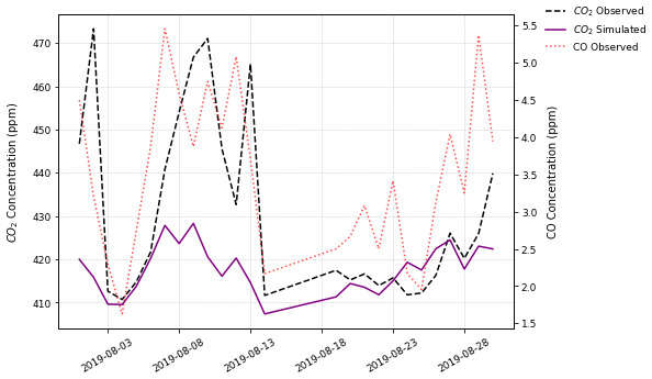
Figure 9 Daily mean concentrations of CO₂, both observed (black dashed line) and simulated (purple line), at the IAG site, along with observed CO concentrations (red dotted line) at the Pinheiros site during August 2019.

3.3.3 Model evaluation against OCO-2 and XCO₂ observations

Figure 10a shows the monthly boxplots of observed and all_sources simulated XCO₂ concentrations for the period from 1 April to 31 August 2019. However, due to insufficient OCO-2 data over MASP during this period, the analysis covers all simulated domains rather than solely the metropolitan area. Regarding temporal variability, a clear seasonal cycle of XCO₂ is evident from its smooth month-to-month variation (green boxes in Fig. 10a). The simulated XCO₂ concentrations, i.e., the simulated profiles with smoothing, generally captured this cycle, although with a less dispersion (length of the box) compared to the observed XCO₂ concentrations. Notably, model–observation discrepancies are most pronounced during the winter months, with differences in median concentrations ranging from 0.8 to 1.5 ppm, while they are minimized during the autumn season, with differences in median concentrations between 0.5 and 0.6 ppm. The simulated XCO₂ concentrations demonstrate similar trends within the same range but tend to slightly underestimate values on most days.

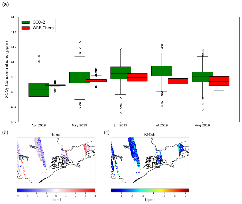
Figure 10 (a) Monthly boxplots of observed and simulated XCO₂ concentrations for the period from 1 April to 31 August 2019; (b) bias and (c) RMSE calculated by pixel over the study domain.

When generating time-averaged modeled values, we only take into account the measurement period as previously mentioned. Regarding XCO₂, the smoothed column concentrations (depicted by red dotted lines in Fig. B9) consistently fall below the observed values on a global scale. Figure 10b and c depict the bias and RMSE, respectively, calculated across the pixel-by-pixel domain. Higher RMSE values are evident in the eastern region of MASP and along the border of the São Paulo and Rio de Janeiro states. In these areas, characterized by heavy vehicular traffic, the model tends to overestimate XCO₂ concentrations. Conversely, for the central region of the domain, we observe slightly negative bias values accompanied by higher RMSE values, indicating an underestimation of XCO₂ concentrations. The uncertainties surrounding XCO₂ simulation stem from various factors, including potential biases in the model's wind representation, particularly in urban areas, consideration of emissions solely at the surface rather than at different pressure levels, and errors in the initial and boundary conditions of concentration provided by CarbonTracker, which has also been seen in other studies (Chen et al., 2019; Lian et al., 2021; Peiro et al., 2022).

4 Conclusions

A comprehensive assessment of atmospheric CO₂ concentrations in the MASP and its surroundings was conducted, utilizing the WRF-Chem model using the greenhouse gas module. Given the burgeoning demand for research in this domain, particularly in South America, where urban areas are marked by significant emission sources, this study aimed to furnish a broad understanding of the key characteristics of CO₂ concentrations. To ensure an accurate estimation of CO₂ levels in MASP, the initial focus of the evaluation was on the model's capability to simulate meteorological variables. Biogenic fluxes were derived from the VPRM model, which was fine-tuned with flux tower data. Our results show that using these local data significantly improved simulated biogenic CO₂ fluxes, highlighted the model's capacity to represent key seasonal dynamics, with negative NEE values predominating in February (summer) and positive values in August (winter). However, we recommend the deployment of additional flux towers and targeted measurement campaigns to improve the characterization other ecosystems. A more comprehensive representation of PFTs is essential, as vegetation processes play a fundamental role in shaping CO₂ patterns in tropical regions. The availability of additional flux tower data would enable a more refined optimization approach, enhancing the characterization of parameters for each vegetation type. Anthropogenic emissions were curated from vehicular model and global inventory to provide a comprehensive representation of urban emissions, incorporating spatial and temporal resolution for key sources such as vehicular traffic for our domain. Boundary and initial conditions were scrutinized using global products. The WRF-Chem model demonstrated skill in simulating meteorological variables, particularly temperature; however, discrepancies in local wind speed and direction persisted. These differences are attributed to the region's complex topography and the model's resolution (3 km), which limits its ability to capture fine-scale dynamical processes.

Simulated CO₂ concentrations exhibited distinct diurnal cycles influenced by local emissions, boundary layer dynamics, and vegetation fluxes. The model's performance varied between monitoring stations, highlighting the interplay between urban and vegetative environments. At the IAG site, CO₂ concentrations were consistently underestimated, with negative biases of −9.17 ppm in February and −12.83 ppm in August. This underestimation was closely linked to the model's difficulty in capturing the impact of high vehicular emission densities, as indicated by the correlation with CO concentrations. Conversely, at the vegetated and elevated PDJ site, the model closely matched observational data, with minimal biases of 0.73 ppm in February and −0.61 ppm in August. In suburban locations such as the PDJ site, distant from urban sources, anthropogenic emissions diminish, and the vertical gradient of CO₂ concentration generated by city emissions attenuates through atmospheric convection and diffusion processes. However, during the growing season, the contribution of biogenic flux to CO₂ concentration warrants attention, especially concerning the simulation of nocturnal CO₂ concentrations and ecosystem respiration. Improvements in the respiration equation of the VPRM model (Gourdji et al., 2022) could enhance the accuracy of these simulations. Importantly, the modeled CO₂ concentrations exhibited high sensitivity not only to atmospheric vertical mixing near the surface but also to the prescribed temporal profiles of anthropogenic and biogenic emissions, highlighting the underestimation of vehicular emissions. These sources of error, particularly pronounced in winter, present challenges in accurately quantifying city emissions.

In general, the WRF-Chem model demonstrated proficiency in simulating seasonal variations, including XCO₂, with profiles akin to OCO-2 data. This study underscores the imperative for further investigations and applications of the WRF-Chem model in uncharted regions such as the MASP, showcasing its prowess in simulating meteorological fields and CO₂ observations.

Appendix A: Metrics evaluation

$$\begin{array}{}\text{(A1)}& {\displaystyle }& {\displaystyle }\mathrm{Bias}={\displaystyle \frac{\sum _{i=\mathrm{1}}^N\left({\mathrm{pred}}_i-{\mathrm{obs}}_i\right)}{N}},\text{(A2)}& {\displaystyle }& {\displaystyle }\mathrm{RMSE}=\sqrt{{\displaystyle \frac{\sum _{i=\mathrm{1}}^N{\left({\mathrm{pred}}_i-{\mathrm{obs}}_i\right)}^{\mathrm{2}}}{N}}},\text{(A3)}& {\displaystyle }& {\displaystyle }{R}^{\mathrm{2}}={\displaystyle \frac{\sum _{i=\mathrm{1}}^N\left({\mathrm{pred}}_i-\stackrel{\mathrm{‾}}{{\mathrm{pred}}_i}\right)\left({\mathrm{obs}}_i-\stackrel{\mathrm{‾}}{{\mathrm{obs}}_i}\right)}{\sqrt{\sum _{i=\mathrm{1}}^N{\left({\mathrm{pred}}_i-\stackrel{\mathrm{‾}}{{\mathrm{pred}}_i}\right)}^{\mathrm{2}}\sum _{i=\mathrm{1}}^N{\left({\mathrm{obs}}_i-\stackrel{\mathrm{‾}}{{\mathrm{obs}}_i}\right)}^{\mathrm{2}}}}},\end{array}$$

where pred_i is the model simulation value, obs_i is the observed value, and N is the number of observations.

Appendix B: Additional figures

This appendix contains figures that give some additional insight to the conclusions given in the sections above and are referenced in the text.

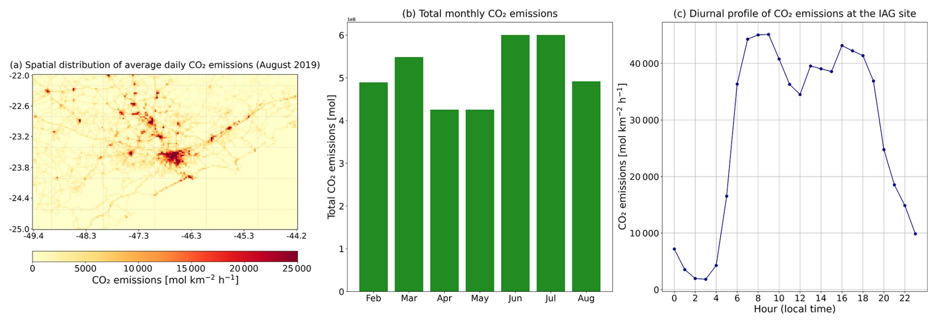
Figure B1 Vehicular CO₂ emissions as estimated by the VEIN model over the study domain (D01). Panel (a) represents the spatial distribution of average daily CO₂ emissions for August 2019 over D01. Panel (b) represents the total monthly CO₂ emissions from February to August 2019 over the D01. Panel (c) shows the diurnal profile of CO₂ emissions at the IAG site during August 2019.

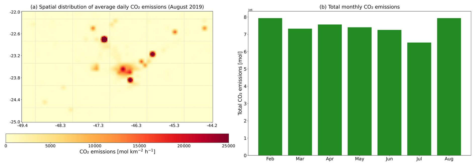
Figure B2 CO₂ emissions from energy, residential, refinery, and industry sectors by the EDGAR inventory over the study domain (D01). Panel (a) shows the spatial distribution of average daily CO₂ emissions for August 2019 over D01. Panel (b) represents the monthly total CO₂ emissions from February to August 2019 over the domain.

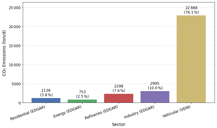
Figure B3 Average daily anthropogenic CO₂ emissions (in tons) for August 2019 within the simulated domain, disaggregated by sector. Bars represent the mean daily emissions per sector, while percentages indicate each sector's relative contribution to total anthropogenic emissions.

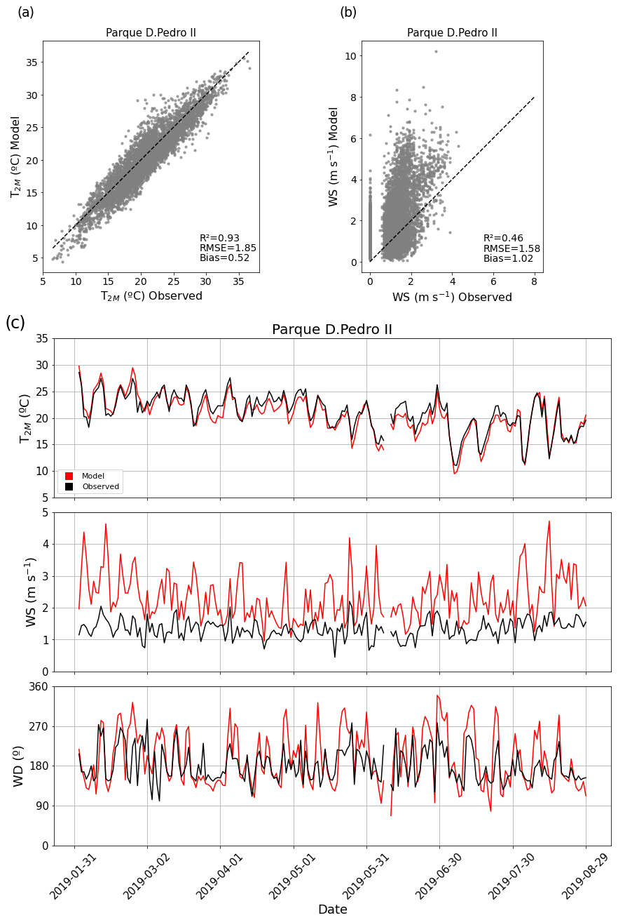
Figure B4 Panels (a) and (b) show scatter plots comparing model outputs and observations at the Parque D. Pedro II station for hourly values of 2 m air temperature (T_2 m) and 10 m wind speed (WS), respectively. Panel (c) presents the daily averages from February to August 2019 for 2 m air temperature (T_2 m), 10 m wind speed (WS), and wind direction (WD). The black line represents observational data, while the red line indicates model simulations.

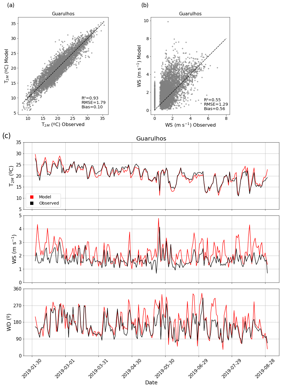
Figure B5 Panels (a) and (b) show scatter plots comparing model outputs and observations at the Guarulhos station for hourly values of 2 m air temperature (T_2 m) and 10 m wind speed (WS), respectively. Panel (c) presents the daily averages from February to August 2019 for 2 m air temperature (T_2 m), 10 m wind speed (WS), and wind direction (WD). The black line represents observational data, while the red line indicates model simulations.

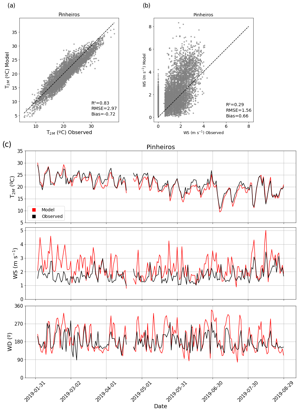
Figure B6 Panels (a) and (b) show scatter plots comparing model outputs and observations at the Pinheiros station for hourly values of 2 m air temperature (T_2 m) and 10 m wind speed (WS), respectively. Panel (c) presents the daily averages from February to August 2019 for 2 m air temperature (T_2 m), 10 m wind speed (WS), and wind direction (WD). The black line represents observational data, while the red line indicates model simulations.

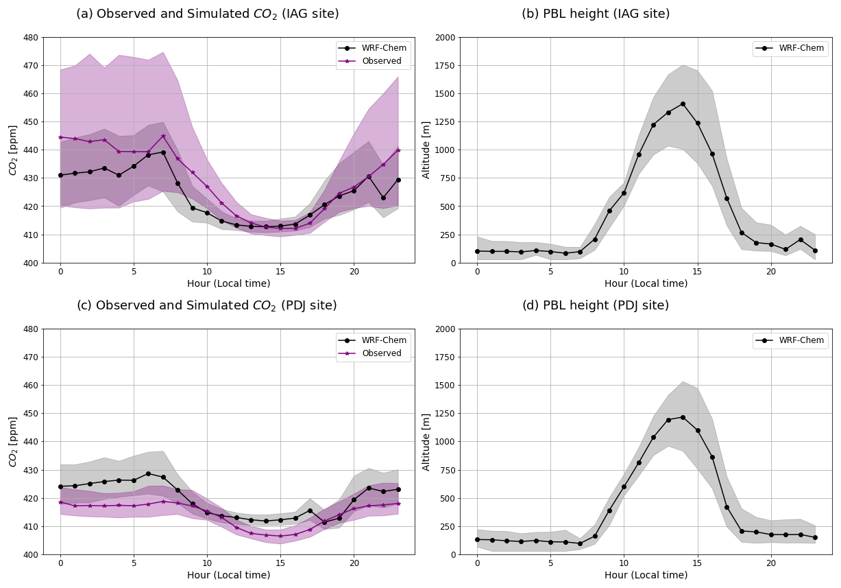
Figure B7 Diurnal cycle of in situ CO₂ concentration and planetary boundary layer (PBL) height for the entire simulated period. The black line represents the median hourly concentrations from WRF-Chem, while the purple line corresponds to the observed values. The shaded areas indicate the interquartile ranges. (a) The observed and simulated surface CO₂ concentration at the IAG site, (b) the simulated PBL height at the IAG site, (c) the observed and simulated surface CO₂ concentration at the PDJ site, and (d) the simulated PBL height at the PDJ site.

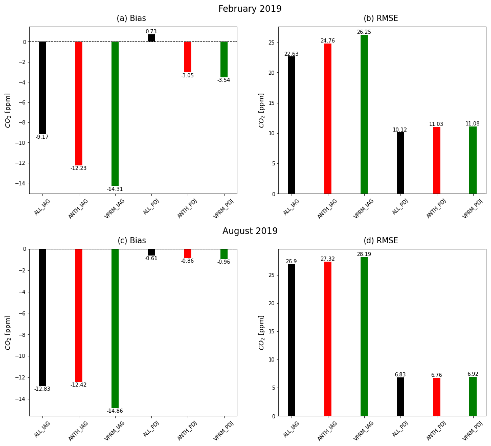
Figure B8 Bias (ppm) and RMSE (ppm) for each simulation at the surface CO₂ observation sites. Panels (a) and (b) represent the simulations for February, while panels (c) and (d) represent the simulations for August (ALL_*: black; ANTH_*: red; VPRM_*: green; the asterisk (^*) represents the observation sites, e.g., IAG and PDJ).

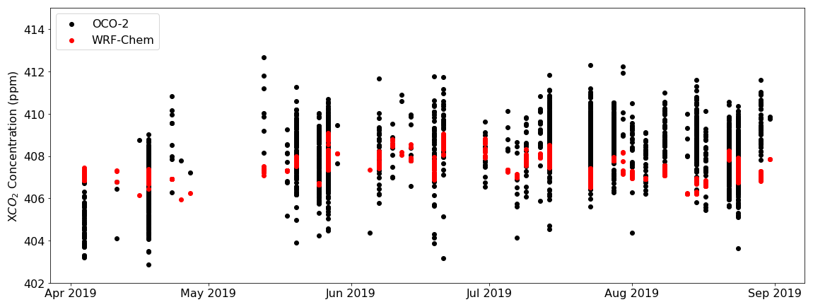
Figure B9 Time series of smoothed column concentrations observed (black) and modeled (red) for the period from 1 April to 31 August 2019.