Subgrid-scale aerosol–cloud interaction in the atmospheric chemistry model CMA_Meso5.1/CUACE and its impacts on mesoscale meteorology prediction

Aerosol–cloud interaction (ACI) significantly influences global and regional weather and is a critical focus in numerical weather prediction (NWP), but subgrid-scale ACI effects are often overlooked. Here, a subgrid-scale ACI mechanism is implemented by explicitly treating cloud microphysics in the KFeta convective scheme with real-time size-resolved hygroscopic aerosol activation and introducing subgrid-scale cloud radiation feedback in an atmospheric chemistry model, CMA_Meso5.1/CUACE. With a focus on summer over central and eastern China, the performance evaluation shows that this developed model with subgrid-scale cloud microphysics and radiation feedback refines cloud representation, even in some grid-scale unsaturated areas, and subsequently leads to attenuated surface downward shortwave radiation (∼ 18.5 W m⁻²) that is more realistic. The increased cloud radiative forcing results in lower temperature (∼ 0.35 °C) and higher relative humidity (∼ 2.5 %) at 2 m, with regional mean bias (MB) decreasing by ∼ 40 % and ∼ 18.1 %. Temperature vertical structure and relative humidity below ∼ 900 hPa are improved accordingly due to cooling and humidifying. The underestimated precipitation is enhanced, especially at the grid scale, thus reducing regional MB by ∼ 34.4 % (∼ 1.1 mm). The performance differences between various subregions are related to convective conditions and model local errors. Additionally, compared to simulations with anthropogenic emissions turned off, subgrid-scale actual aerosol inhibits cumulative precipitation during a typical heavy rainfall event by ∼ 4.6 mm, aligning it with observations, associated with lower autoconversion at the subgrid scale and less available water vapor for grid-scale condensation, suggesting competition between subgrid- and grid-scale cloud. This study contributes to the understanding of the impact of subgrid-scale ACI on NWP.

1 Introduction

Cloud plays an essential role in climate and weather by maintaining the atmospheric radiation balance, regulating global precipitation, facilitating chemical reactions, etc. (Pruppacher and Klett, 1980; Seinfeld and Pandis, 2006; Fan et al., 2016). In the actual atmosphere, water vapor is hardly able to form cloud droplets spontaneously due to the free-energy barrier until the heterogeneous nucleation process is completed with the help of suspended aerosol particles (Seinfeld and Pandis, 2006; Sun and Ariya, 2006). The perturbation of aerosol particles inevitably affects cloud properties, also known as aerosol–cloud interaction (ACI), including the Twomey effect (Twomey, 1977) and the Albrecht effect (Albrecht, 1989). Due to the complexity of cloud and aerosol processes and their entangled nature, ACI is still subject to significant uncertainties in current climate projections and weather forecasts (IPCC, 2021, 2013; Miltenberger et al., 2018; Baklanov et al., 2017). In the latest Intergovernmental Panel on Climate Change (IPCC) report, ACI has the lowest confidence in effective radiative forcing estimates (IPCC, 2021).

Compared to the extensive research in the climate modeling community, ACI is less considered among various numerical weather prediction (NWP) models (Rosenfeld et al., 2014; Wang et al., 2014; Seinfeld et al., 2016). The NWP model runs daily in major regional operational centers worldwide and is primarily responsible for weather forecasts. For a long time, operational NWP models have been based on seven fundamental equations of atmospheric motion to predict future atmospheric states, with few considerations of the aerosol effect, especially of ACI, on meteorology due to the cognitive and computing power required (Grell and Baklanov, 2011; Sandu et al., 2013; Pleim et al., 2014; Baklanov et al., 2017). An aerosol climatology used in the NWP model may mitigate the forecast bias but cannot represent actual aerosol levels (Thompson and Eidhammer, 2014; Song and Zhang, 2011). The NWP models with “two-way” feedback between chemistry and meteorology (e.g., the Weather Research and Forecasting model coupled with Chemistry (WRF-Chem) and the Weather Research and Forecasting and Community Multiscale Air Quality (WRF-CMAQ)) can fill this gap and have been widely applied to multiscale studies to investigate the role of ACI in reducing radiation, cooling temperature, inhibiting or enhancing precipitation, etc. (Zhang et al., 2010; Grell and Baklanov, 2011; Wong et al., 2012; Makar et al., 2015; Zhang et al., 2015; Han et al., 2023). These studies have explicitly addressed the fact that ACI has an essential influence on weather systems but have rarely focused on its feedback on NWP. With the rapid development of supercomputing technology and the keen concerns about the impacts of anthropogenic activity on weather, the role of ACI in NWP is only beginning to be scrutinized in detail (Zhang et al., 2022; Zhang et al., 2024; Wang et al., 2021). For example, Zhang et al. (2024) show that the coupling of real-time hygroscopic aerosol activation in the Thompson cloud microphysics scheme in an atmospheric chemistry model, CMA_Meso5.1/CUACE, improves the accuracy of predicted surface and vertical meteorological factors during the low-cloud period in winter in China.

To the best of our knowledge, almost all of the studies in this area focus on ACI at the grid scale. An important reason for this is that cloud microphysics schemes in NWP models include explicit cloud microphysics processes and aerosol activation, whereas cumulus convection schemes do not. Cumulus convection schemes in mesoscale NWP models are designed to better characterize subgrid-scale cloud processes that are not directly resolved (Arakawa, 2004; Plant, 2010); typical examples of these are the Kain–Fritsch (KF) scheme (Kain and Fritsch, 1993) and the follow-up KFeta scheme (Kain, 2004), the KFcup scheme (Berg et al., 2013), and the MSKF scheme (Zheng et al., 2016). These schemes are mass-flux parameterizations that use grid-scale information to determine the conditions under which convection occurs, include cloud models for both updrafts and downdrafts, and allow cumulus feedback for grid-scale cloud. Notably, during the periods of strong small-scale convections, only considering grid-scale ACI potentially overlooks the effect of aerosol on convective clouds that are not resolvable at the grid scale, further affecting the assessment of the role of ACI in NWP. Cumulus convection schemes that include detailed cloud microphysical processes must be incorporated into the NWP model. Lohmann (2008) extended the double-moment cloud microphysics scheme developed for stratiform cloud in the ECHAM5 global climate model (GCM) to convective cloud (mainly for cloud droplets and ice crystals) and found a significant increase in simulated convective precipitation. Grell and Freitas (2014) developed a scale- and aerosol-aware stochastic convective parameterization based on a cumulus scheme only including liquid-phase processes and demonstrated the importance of a changed autoconversion mechanism for precipitation through preliminary experiments with cloud condensation nuclei (CCN) concentration perturbations. To address aerosol–convective cloud simulations in global climate models (GCMs), Song and Zhang (2011) proposed a double-moment convective cloud microphysics scheme (SZ2011) containing a detailed treatment of four hydrometeor species. Lim et al. (2014) found that implementing the SZ2011 scheme in the new Zhang and McFarlane (ZM) cumulus scheme improves simulated precipitation and radiation. Recently, Glotfelty et al. (2019) implemented the SZ2011 scheme with climatological aerosol concentrations into the MSKF scheme and further considered the radiative feedback of subgrid-scale cloud in the WRF model, which improves the simulation of cloud properties and precipitation. It is worth noting that climatological aerosol that differs spatially and temporally from real-time predicted aerosol exacerbates uncertainty in ACI, especially at the subgrid scale, where the ACI appears to be more strongly represented at the subgrid scale compared to at the grid scale (Glotfelty et al., 2019, 2020).

To investigate the impact of subgrid-scale ACI, a double-moment convective cloud microphysical scheme including real-time hygroscopic aerosol activation is coupled into the KFeta cumulus convection scheme in an atmospheric chemistry model, CMA_Meso5.1/CUACE; the impact of the treatment of subgrid-scale cloud microphysics and radiation feedback on multiple predicted meteorological factors is systematically evaluated; and the role of anthropogenic aerosol activation at the subgrid scale in deep-convective precipitation is further discussed. The innovativeness of this study lies in establishing a complete process chain from emissions to aerosol; to subgrid-scale cloud; and, ultimately, to radiation and/or precipitation in an atmospheric chemistry model, which allows for the impact of subgrid-scale ACI on meteorology prediction (e.g., cloud, radiation, temperature, and precipitation) to be investigated at a more realistic aerosol level. The overall goal of this study is to achieve quantifiable subgrid-scale ACI in the atmospheric chemistry model CMA_Meso5.1/CUACE and to understand the impact of subgrid-scale ACI on meteorology prediction.

2 Data

The data used in this paper are as follows: (1) aerosol pollution observation data, with hourly PM_2.5 mass concentrations (µg m⁻³) coming from more than 1300 air pollution stations of the Ministry of Ecology and Environment of the People's Republic of China; (2) near-surface meteorological observation data, with hourly temperature at 2 m (T2m, °C), relative humidity (RH) at 2 m (RH2m, %), wind speed at 10 m (WS10m, m s⁻¹), and 24 h cumulative precipitation (PRE24h, mm) being provided by more than 5000 automated weather stations of the China Meteorological Administration (CMA) (Fig. 1); (3) vertical meteorological observation data, for which, twice a day (00:00 and 12:00 UTC) temperature, RH, and WS are monitored by L-band radar from about 85 sounding stations of the CMA (Fig. 1); (4) radiation observation data, with hourly surface downward shortwave radiation (SDSR, 0.01 MJ m⁻²) in the daytime being obtained from more than 70 radiation stations of the CMA (Fig. 1); (5) satellite data, with daily cloud fraction (CF, %), cloud liquid-water path (CLWP, g m⁻²), and cloud optical thickness (COT) coming from the Suomi National Polar-orbiting Partnership (SNPP) Visible Infrared Imaging Radiometer Suite (VIIRS) (the daily cloud property data from VIIRS used in this study consist solely of visible-band products, which are available only during the local daytime; the daily SDSR (W m⁻²) and surface downward longwave radiation (SDLR, W m⁻²) come from the Clouds and the Earth's Radiant Energy System (CERES), with the horizontal resolution of these data being 1° × 1°, and the daily radiation properties from CERES are computed with hourly data derived from Moderate Resolution Imaging Spectroradiometer (MODIS) and geostationary satellites (GEO), while Daily PRE24h (mm) data are from the Global Precipitation Measurement (GPM) program's Integrated Multi-satellitE Retrievals (IMERG), with a horizontal resolution of 10 km × 10 km); (6) hourly aerosol optical depth (AOD) data come from the Modern-Era Retrospective analysis for Research and Applications version 2 (MERRA-2) dataset, with a horizontal resolution of 0.5° × 0.625°; (7) re-analysis data, with the final (FNL) operational global analysis and forecast data, with a horizontal resolution of 0.25° × 0.25° and a time interval of 6 h, coming from the National Centers for Environmental Prediction (NECP)/National Center for Atmospheric Research (NCAR) (these data are primarily produced by the Global Data Assimilation System (GDAS), which continuously collects observations from the Global Telecommunications System (GTS) and other sources); and (8) emission data, with the Multi-Resolution Emission Inventory for China (MEIC) anthropogenic emission data being provided by Tsinghua University, including six sectors (power, industry, civil, transportation, and agriculture) and nine species (SO₂, NO_x, CO, non-methane volatile organic compounds (NMVOCs), NH₃, PM₁₀, PM_2.5, black carbon (BC), and organic carbon (OC)).

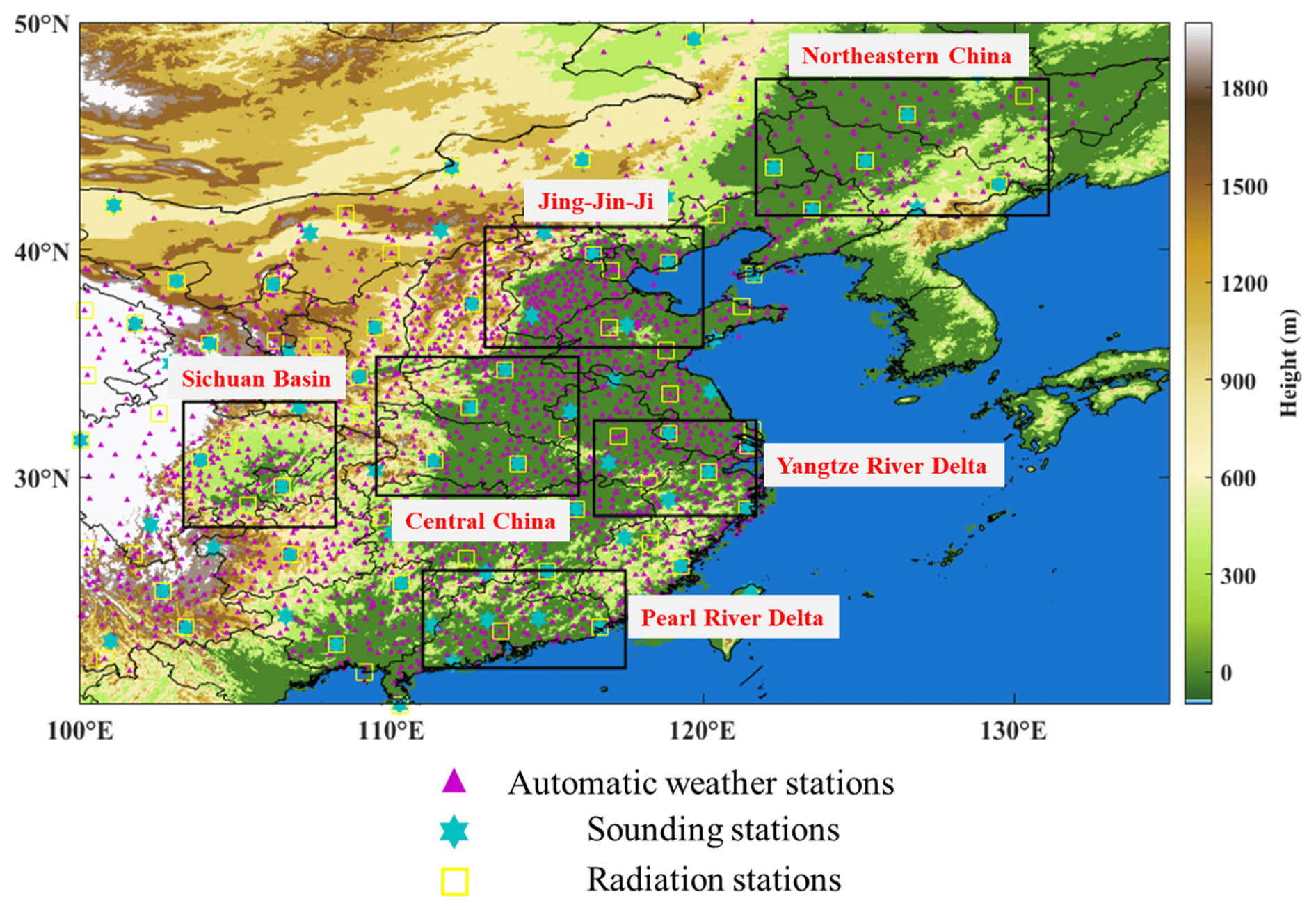
Figure 1 The map and topographic height of the simulated domain. The purple triangles are the automatic weather stations; the cyan hexagons are the sounding stations; the yellow boxes are the radiation sounding stations; and the black rectangles represent the locations of northeastern China (NEC), Jing-Jin-Ji (JJJ), the Sichuan Basin (SB), central China (CC), the Yangtze River Delta (YRD), and the Pearl River Delta (PRD).

3 Model description and development

3.1 CMA_Meso5.1/CUACE model

The CMA_Meso/CUACE model, independently developed by the CMA, is online, coupled with a mesoscale NWP model (China Meteorological Administration Mesoscale model version 5.1 (CMA_Meso5.1)) and with an atmospheric chemistry module (Chinese Unified Atmospheric Chemistry Environment (CUACE)), which has been widely used for studying the ARI effects on aerosol pollution, the transboundary transport of air pollutants (Jiang et al., 2015), the impacts of anthropogenic emissions on PM_2.5 changes (Wang et al., 2018; Zhang et al., 2020), visibility forecasts (Peng et al., 2020; Han et al., 2024), fog–haze forecasts (Zhou et al., 2012; Wang et al., 2015b; Wang et al., 2015a; Li et al., 2023), etc. In this study, the latest quasi-operational version, CMA_Meso5.1/CUACE, is used, and its specific updates can be found in a previous study (Wang et al., 2022).

The CMA_Meso5.1 is a continuous development of the GRAPES_Meso, mainly including pre-processing and quality control, standard initialization, assimilation and forecasting, and post-processing, and it is used to meet the operational needs of the short-term weather forecasting in China (Chen and Shen, 2006; Chen et al., 2008; Zhang and Shen, 2008). In this model, the temporal, horizontal, and vertical discretizations adopt the semi-implicit semi-Lagrangian scheme, Arakawa C-grid staggering, and Charney–Phillips staggering, respectively. This model also contains a series of physical parameterization schemes, such as radiation, boundary layer, near-surface layer, cumulus convection, and cloud microphysical schemes.

The CUACE is an atmospheric chemistry module that includes the emission treatment system, the gas and aerosol calculation processes, and the thermodynamic equilibrium module (Zhou et al., 2012; Wang et al., 2015b). There are seven types of aerosol: sulfates (SF), road dust (RD), black carbon (BC), organic carbon (OC), sea salts (SS), nitrates (NI), and ammonium (AM). All types of aerosol radii except AM are categorized into 12 bins ranging from 0.005 to 20.48 µm. Aerosol calculation processes include hygroscopic growth, wet and dry deposition, chemical transformations, and coagulation. The 63 species of gases in the CUACE are calculated and updated by 21 photochemical and 136 gas-phase chemical reactions.

3.2 Grid-scale ACI

Before dealing with subgrid-scale ACI, it is necessary to describe the grid-scale ACI implemented based on the double-moment Thompson cloud microphysics scheme in the current model. The original assumed cloud droplet number concentration (100 cm⁻³) in the Thompson cloud microphysics scheme is replaced by the predicted value, which is determined based on the activation fraction of real-time calculated hygroscopic aerosol (OC, SS, SF, NT, and AM) in CUACE by using the look-up table; the fixed cloud water (10 µm) and cloud ice (80 µm) radii in the Goddard shortwave radiation scheme are replaced by diagnosed values in the Thompson cloud microphysics scheme. More detailed descriptions can be found in a previous study (Zhang et al., 2022). In this study, we do not conduct an extra consistent treatment of the grid-scale ACI because of the ability to understand the impact of subgrid-scale ACI and the convenience of comparison with the previous study.

3.3 Implementation of subgrid-scale ACI

3.3.1 Coupling of the double-moment microphysics parameterization scheme for convective cloud in the KFeta cumulus convection scheme

Optional cumulus convection parameterization schemes in the current model include the BMJ (Betts, 1986; Betts and Miller, 1986; Janjić, 1994), KFeta (Kain, 2004), NSAS (Han and Pan, 2011), and Tiedtke (Tiedtke, 1989) schemes. To implement subgrid-scale ACI, an efficient double-moment microphysics parameterization scheme for convective cloud is coupled with the commonly used KFeta cumulus convection scheme.

The KFeta scheme is a typical cumulus convection scheme used in the mesoscale NWP model, whose fundamental framework is derived initially from the Fritsch–Chappell convective parameterization scheme (Fritsch and Chappell, 1980). The classic KF scheme (Kain and Fritsch, 1993) has evolved through a series of modifications into the KFeta scheme, including imposed minimum entrainment rate, variable cloud radius, variable minimum cloud depth threshold, and allowed shallow convection (Kain, 2004). However, its treatment of convective cloud microphysical processes is rather crude, especially for the transformations between the various hydrometeors within the convective cloud. At the same time, it is a mass-flux parameterization scheme, which can correspond well with the double-moment microphysics parameterization scheme for convective cloud.

This double-moment microphysics parameterization scheme for convective cloud is proposed by Song and Zhang (2011) to improve the performance of convective cloud interacting with stratiform cloud and aerosol in GCMs. The mixing ratio and number concentration of cloud water, cloud ice, rain, and snow can be simultaneously predicted. Figure 2 shows the microphysical processes of these four hydrometeors in the double-moment microphysics parameterization scheme, mainly including autoconversion, freezing, accretion, self-collection, detrainment, fallout, aerosol activation, and ice nucleation. The detailed control equations and microphysical process calculations for each hydrometeor can be found in a previous study (Song and Zhang, 2011). The real-time activation of aerosol as CCN to cloud droplets is carried out by means of the ARG2000 scheme (Abdul-Razzak and Ghan, 2000; Abdul-Razzak et al., 1998), as detailed in Sect. 3.3.2. The current scheme does not include real-time ice nucleation because the dust is not available in the CUACE model. The ice crystal number concentration can be derived using Eq. (1) as proposed by Cooper (1986):

$$\begin{array}{}\text{(1)}& \mathrm{sub}\mathrm{\_}\mathrm{Ni}=\mathrm{0.005}{e}^{\mathrm{0.304}(\mathrm{273.15}-T)},\end{array}$$

where sub_Ni is the ice crystal number concentration (L), and T is the simulated ambient temperature (K) at the subgrid scale. It should be noted that ice crystals can only form when the supersaturation with respect to ice exceeds 5 % or when the supersaturation with respect to water exceeds 0 and when the ambient temperature is < −5°C, consistently with that in the Thompson cloud microphysics scheme (Thompson and Eidhammer, 2014). Considering a reduction in the complexity of the code and additional errors, we directly couple the SZ2011 scheme with the KFeta scheme via a one-to-one correspondence of specific values, such as cloud water mixing ratio, cloud ice mixing ratio, rate of production of precipitation, and rate of production of snow. It should be noted that the grid-scale hydrometeors are calculated separately, and the subgrid-scale hydrometeors are only fed back to influence the grid-scale hydrometeors through the detrainment and entrainment processes.

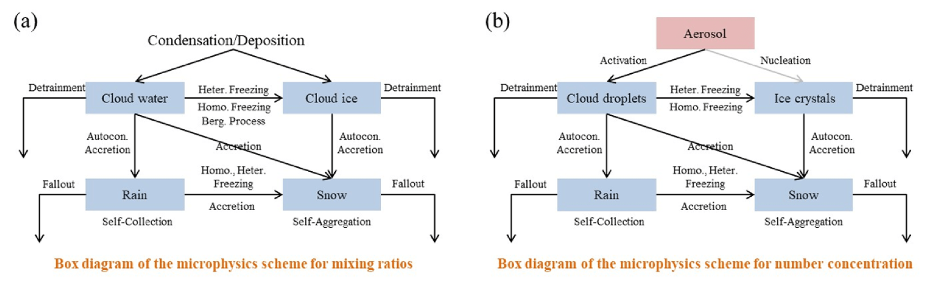
Figure 2 Box diagram of microphysical processes for various hydrometeor mixing ratios (a) and number concentrations (b) in the SZ2011 double-moment microphysics parameterization scheme for convective cloud. The real-time ice nucleation is not available.

3.3.2 The real-time aerosol activation process

To implement real-time aerosol activation as CCN at the subgrid scale, the subgrid-scale cloud droplet number concentration from the ARG2000 scheme (Abdul-Razzak and Ghan, 2000), driven by predicted hygroscopic aerosol in the CUACE model, is integrated into the KFeta scheme with the SZ2011 parameterization (Fig. 3). The ARG2000 scheme is an activation scheme of aerosol with divided components and a divided size, and it is widely used in mesoscale NWP models. This parameterization is suitable for seven types of aerosol with 12 bins as predicted by the CUACE module and described using the following equations:

$$\begin{array}{}\text{(2)}& {\displaystyle }\mathrm{sub}\mathrm{\_}\mathrm{Nc}={\sum }_{\mathrm{num}=\mathrm{1}}^{\mathrm{49}}{N}_{\mathrm{anum}}{\displaystyle \frac{\mathrm{1}}{\mathrm{2}}}\left[\mathrm{1}-\mathrm{erf}\left({\displaystyle \frac{\mathrm{2}\ln (S_{\mathrm{mnum}}/S_{\max })}{\mathrm{3}\sqrt{\mathrm{2}}\ln {\mathit{\sigma }}_{\mathrm{num}}}}\right)\right],\text{(3)}& {\displaystyle }\begin{array}{rl}& S_{\max }=\\ & {\displaystyle \frac{\mathrm{1}}{{\left\{{\sum }_{\mathrm{num}=\mathrm{1}}^{\mathrm{49}}\frac{\mathrm{1}}{S_{\mathrm{mnum}}^{\mathrm{2}}}\left[\left(\mathrm{0.5}{e}^{\mathrm{2.5}{\ln }^{\mathrm{2}}{\mathit{\sigma }}_{\mathrm{num}}}\right){\left(\frac{\mathit{\zeta }}{{\mathit{\eta }}_{\mathrm{num}}}\right)}^{\mathrm{1.5}}+(\mathrm{1}+\mathrm{0.25}\ln {\mathit{\sigma }}_{\mathrm{num}}){\left(\frac{S_{\mathrm{mnum}}^{\mathrm{2}}}{{\mathit{\eta }}_{\mathrm{num}}+\mathrm{3}\mathit{\zeta }}\right)}^{\mathrm{0.75}}\right]\right\}}^{\mathrm{0.5}}}}\end{array},\text{(4)}& {\displaystyle }{S}_{\mathrm{mnum}}={\displaystyle \frac{\mathrm{2}}{{\sqrt{b}}_{\mathrm{num}}}}{\left({\displaystyle \frac{{\mathrm{3.2910}}^{-\mathrm{7}}}{\mathrm{3}{r}_{\mathrm{num}}T}}\right)}^{\mathrm{1.5}},\end{array}$$

where, in Eq. (2), sub_Nc is the subgrid-scale cloud droplet number concentration (kg⁻¹) generated by activation, N_anum is the aerosol number concentration (kg⁻¹), S_max is the maximum supersaturation, S_mnum is the critical supersaturation for aerosol activation, σ_num is the aerosol geometric standard deviation, erf is the Gaussian error function, and num is the aerosol type ranging from 1 to 49 (Table 1). S_max can be solved by means of Eq. (3), where ζ and η are two dimensionless parameters given by Abdul-Razzak and Ghan (2000). S_mnum can be solved by means of Eq. (4), where b_num is the aerosol hygroscopicity parameter, r_num is the aerosol mean radius (µm), and T is the ambient temperature (K).

In general, the solution of the activation fraction requires inputs of meteorological factors and aerosol parameters. Meteorological factors include subgrid-scale vertical velocity (w_sub) and temperature, which can be provided in real time by the CMA_Meso5.1 model. The w_sub is determined by the updraft kinetic energy (K_sub), described using the following equations:

$$\begin{array}{}\text{(5)}& {\displaystyle }{w}_{\mathrm{sub}}=\sqrt{\mathrm{2}{K}_{\mathrm{sub}}},\text{(6)}& {\displaystyle \frac{\partial K_{\mathrm{sub}}}{\partial \mathrm{z}}}=-{\displaystyle \frac{v_{\mathrm{w}}}{{\mathrm{M}}_{\mathrm{w}}}}\left(\mathrm{1}+\mathit{\beta }{C}_{\mathrm{d}}\right)K_{\mathrm{sub}}+{\displaystyle \frac{\mathrm{1}}{f(\mathrm{1}+\mathit{\lambda })}}g{\displaystyle \frac{T_{\mathrm{wu}}-T_{\mathrm{we}}}{T_{\mathrm{wu}}}},\text{(7)}& {\displaystyle }{T}_{\mathrm{wu}}=T_{\mathrm{u}}(\mathrm{1}+\mathrm{0.608}\mathrm{Qu}-\mathrm{Qr}-\mathrm{Qi}-\mathrm{Qc}-\mathrm{Qs})\text{(8)}& {\displaystyle }{T}_{\mathrm{we}}=T_{\mathrm{e}}(\mathrm{1}+\mathrm{0.608}\mathrm{Qe}),\end{array}$$

where v_w is the larger of the entrainment or detrainment mass flux, and M_w is the convective updraft mass flux in the KFeta scheme. β, C_d, λ, and f are constants, which are set to 1.875, 0.506, 0.5, and 2, and g is the gravitational acceleration. T_wu and T_we are the density temperature of the updraft and the environment, which can be solved by Eqs. (7) and (8). In Eq. (7), T_u is the temperature of the updraft, Qu is the specific humidity of the updraft, and Qr (Qi, Qc, or Qs) is the rain (ice, cloud, or snow) water mixing ratio. In Eq. (8), T_e is the temperature of the environment, and Qe is the specific humidity of the environment. The calculation of the subgrid-scale vertical velocity can be conducted using the method in Sect. 2.2 of the study by Song and Zhang (2011). The minimum value of the subgrid-scale vertical velocity is set to 0.5 m s⁻¹ at the cloud base, and the maximum value is less than 20 m s⁻¹.

Table 1 The specific values of the tracer number, aerosol types, mean radius (µm), density (g cm⁻³), geometrical standard deviation (GSD), and hygroscopicity parameter.

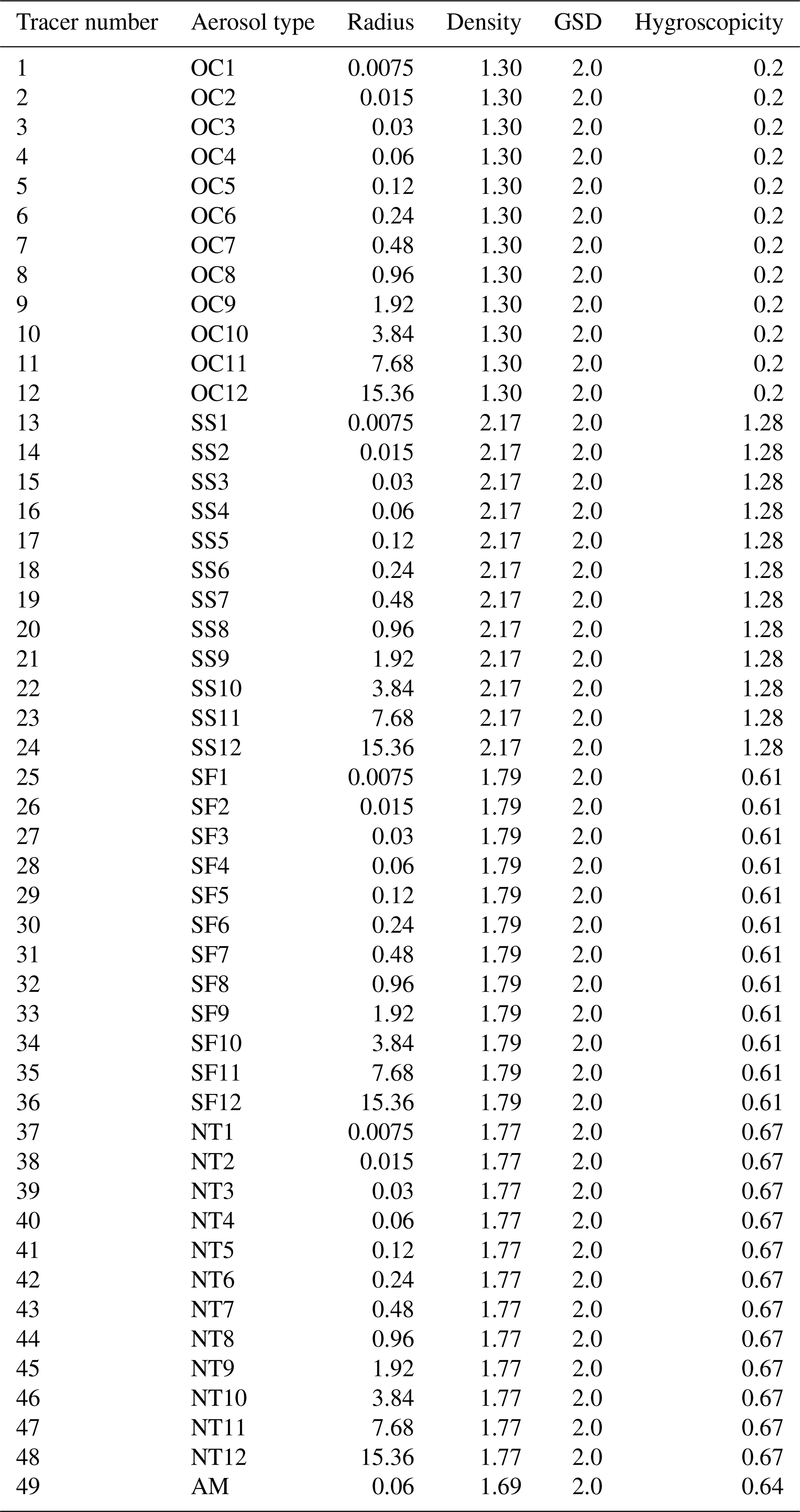
Aerosol parameters include aerosol number concentration, mass concentration, geometric standard deviation, density, and size. The CUACE module only outputs the aerosol mass mixing ratio and not the number concentration. Under the assumption that aerosol particles are spherical, each type of aerosol number concentration is obtained by means of Eq. (9):

$$\begin{array}{}\text{(9)}& N_{\mathrm{anum}}={\mathrm{tracer}}_{\mathrm{num}}/\left({\displaystyle \frac{\mathrm{4}}{\mathrm{3}}}\cdot \mathit{\pi }\cdot r_{\mathrm{num}}^{\mathrm{3}}\cdot {\mathit{\rho }}_{\mathrm{num}}\right),\end{array}$$

where tracer_num is the aerosol mass mixing ratio (kg kg⁻¹) generated by the CUACE model, and ρ_num is the aerosol density (g cm⁻³). All other aerosol parameters are preset: the density and radius are shown in Table 1; the geometric standard deviation is set to 2.0 for all types of aerosol; and the hygroscopicity parameters are set to 0.2, 1.28, 0.61, 0.67, and 0.64 for OC, SS, SF, NT, and AM, respectively. The hygroscopicity parameter for OC is slightly higher than the typical value of 0.1, which was attributed to the fact that the region of China is frequently hazed (Petters and Kreidenweis, 2007; Che et al., 2017). The hygroscopicity parameters of SS, SF, NT, and AM are similar to those of other studies (Kim et al., 2021; Morales Betancourt and Nenes, 2014; Petters and Kreidenweis, 2007). Identically to the grid-scale ACI mechanism, BC and RD, two non-hygroscopic aerosol, are not used as the subgrid-scale aerosol to be activated. It should be noted that cloud droplets can only form when the supersaturation with respect to water exceeds 0.

3.3.3 The feedback of subgrid-scale cloud to radiation

In order to represent the impact of subgrid-scale ACI on radiation, this study completed the feedback of subgrid-scale cloud properties on radiation by coupling subgrid-scale CF, Qc, Qi, cloud water effective radius (Rc), and cloud ice effective radius (Ri) with the Goddard shortwave radiation scheme (Fig. 3). It should be noted that the grid-scale CF, Qc, and Qi are the default inputs into the Goddard shortwave radiation scheme, and Rc and Ri at the grid scale are based on the diagnostics of the Thompson cloud microphysics scheme and have also been coupled with the radiation scheme used in a the previous study (Zhang et al., 2022). The subgrid-scale CF is calculated with reference to CAM5 (Neale et al., 2012; Xu and Krueger, 1991), where the CF values for deep convection and shallow convection have been estimated separately using the KFeta scheme. These two types of CF values have been added directly to the grid-scale CF, keeping the total CF range between 0 and 1. The subgrid-scale Qc and Qi are derived from the SZ2011 scheme and are combined with the grid-scale Qc and Qi with reference to a previous study (Alapaty et al., 2012). The subgrid-scale Rc and Ri are also derived from the SZ2011 scheme, which is combined with the grid-scale Rc and Ri based on the studies of Thompson et al. (2016) and Glotfelty et al. (2019). The adjusted CF, Qc, Qi, Rc, and Ri in the Goddard shortwave radiation scheme simultaneously incorporate cloud properties at both the grid scale and the subgrid scale.

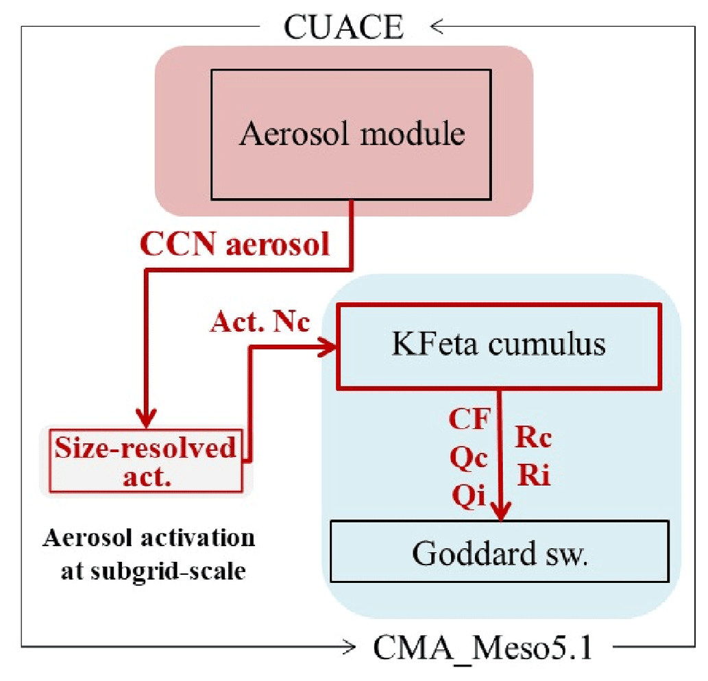
Figure 3 The diagram of subgrid-scale aerosol–cloud–radiation interaction in the CMA_Meso5.1/CUACE model.

4 Model configurations and experimental design

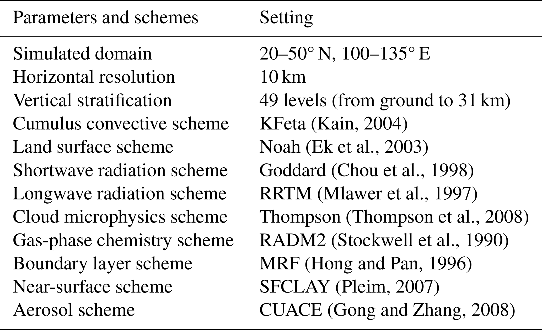
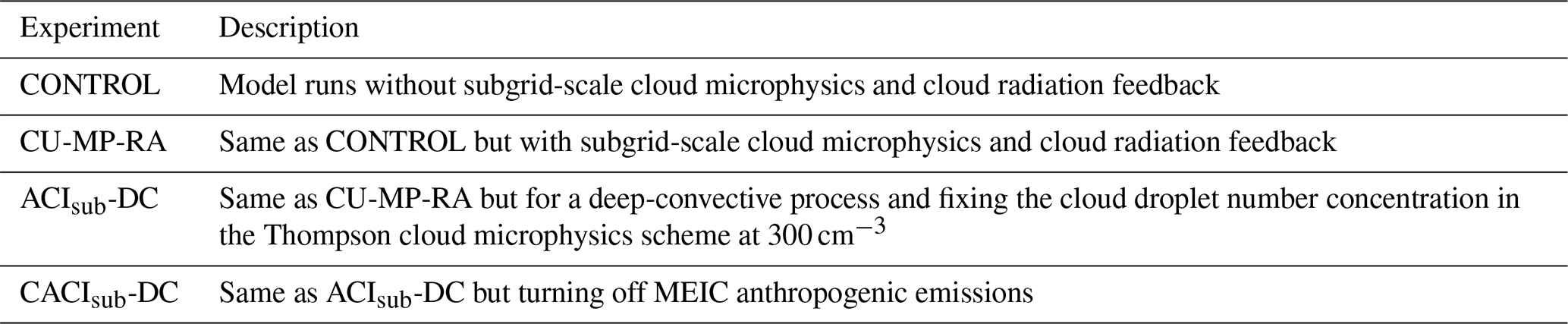
In this study, two sets of experiments are conducted using the CMA_Meso5.1/CUACE model to evaluate the performance of the developed model with subgrid-scale cloud microphysics and radiation feedback. In the first set of experiments, the CONTROL and CU-MP-RA experiments are included to focus on the summer of 2016 (June represents the summer season), when convection occurs more frequently in China and when the water vapor conditions are better, focusing on the NEC, JJJ, SC, CC, YRD, and PRD regions (Fig. 1). The average of these six regions is used to represent the entirety of central and eastern China. For the CONTROL experiment, the model configurations are shown in Table 2. These settings are the same as in a previous study (Zhang et al., 2022). The CU-MP-RA experiment contains all of the treatments of the relevant subgrid-scale ACI mechanisms in Sect. 3.3, except the other settings are the same as in the CONTROL experiment (Table 3). The difference between the CU-MP-RA and CONTROL experiments shows the changed performance in terms of the predicted meteorological factors in the current model due to subgrid-scale cloud microphysics and radiation feedback. The simulated periods of both experiments are from 29 May to 30 June 2016, with a forecast time of 24 h, a time step of 100 s, and an output interval of 1 h. The 72 h pre-simulations are used to keep a balance between the chemical initial field and the meteorological field and are treated as the spin-up time. In the second set of experiments, the ACI_sub-DC and CACI_sub-DC experiments are included to study the impact of anthropogenic aerosol on cloud and precipitation via the subgrid-scale ACI mechanism, mainly for a typical deep-convective heavy-precipitation process (from 26 to 29 June 2016). The settings of the ACI_sub-DC experiment are the same as those of the CU-MP-RA experiments, except for the fixed cloud droplet number concentration (300 cm⁻³) in the Thompson cloud microphysics scheme, which can prevent the additional uncertainties from anthropogenic aerosol affecting the grid-scale ACI. In the CACI_sub-DC experiment, the MEIC anthropogenic emissions are turned off in the model, and other settings are the same as those of the ACI_sub-DC experiment (Table 3). The difference between ACI_sub-DC and CACI_sub-DC indicates the impact of anthropogenic aerosol via the subgrid-scale ACI. The simulated periods of both experiments are from 23 to 30 June 2016, with a forecast time of 48 h. The first 72 h of simulations are also treated as the spin-up time. The initial field and boundary conditions for meteorology are provided by the FNL data, which are the same as those of the time period simulated for each set of experiments. The anthropogenic emission data in June 2016 entered into the model are from the MEIC.

Table 2 Model configurations.

Table 3 Descriptions of multiple sensitivity experiments.

5 Results and discussion

5.1 Evaluations of PM_2.5 mass concentration and aerosol optical depth

To assess the performance of the CMA_Meso5.1/CUACE model in terms of aerosol prediction, Fig. 4 shows the comparisons of the spatial distributions of the observed and simulated time average PM_2.5 mass concentrations and aerosol optical depth (AOD) in June 2016. As shown, the observed PM_2.5 mass concentration over widespread areas of the domain is almost below 75 µg m⁻³, with the regional average PM_2.5 mass concentration being 26.4, 47.9, 33.6, 37.3, 35.8, and 19.4 µg m⁻³ in the NEC, JJJ, SB, CC, YRD, and PRD regions. The model reproduces the spatial distribution of the high-value and low-value areas of PM_2.5 mass concentration and captures the magnitude of PM_2.5 mass concentration at most air quality monitoring stations. The mean bias (MB) of regional average PM_2.5 mass concentration is −12.2, −16.3, 3.2, 0.9, −2.9, and −2.9 µg m⁻³ in the NEC, JJJ, SB, CC, YRD, and PRD regions, respectively. Here, the AOD represents the column-integrated aerosol properties. The MERRA-2 data show that the regional average AOD is 0.42, 0.62, 0.35, 0.50, 0.52, and 0.27 in the NEC, JJJ, SB, CC, YRD, and PRD regions, respectively. The CMA_Meso5.1/CUACE model seems to capture some high-value and low-value areas of AOD well in the south of the domain (e.g., the regional average AOD is 0.31, 0.41, and 0.20 in the SB, YRD, and PRD, with MB values of −0.04, −0.11, and −0.07) but significantly underestimates AOD in the north of the domain (e.g., the regional average AOD is 0.14, 0.28, and 0.32 in the NEC, JJJ, and CC regions, with MB values of −0.28, −0.34, and −0.18). This substantially underestimated AOD in the NEC and JJJ regions, accompanied by the underestimated PM_2.5 mass concentration, is possibly related to underestimated anthropogenic emissions, inadequate representation of aerosol chemical reaction processes, etc. Compared with other studies or models, the CMA_Meso5.1/CUACE model shows a similar performance in predicting AOD over China in summer (Werner et al., 2019; Wang et al., 2021; He et al., 2022). This study's relatively reliable aerosol simulation performance can ensure the scientificity of further subgrid-scale ACI studies.

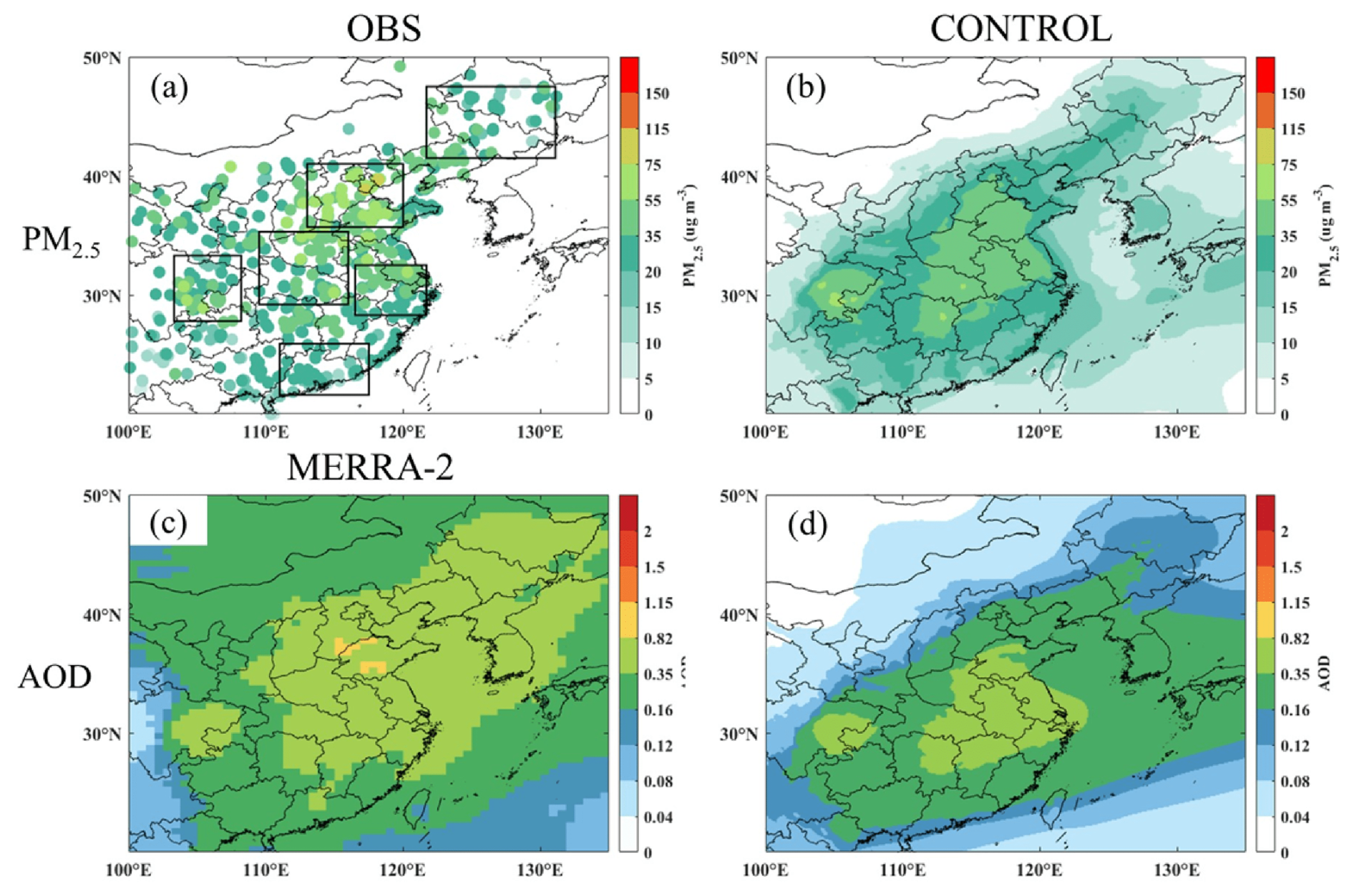
Figure 4 Spatial distribution of time-averaged PM_2.5 (a, b) and AOD (c, d) in June 2016 from the CONTROL experiment compared against the observations and MERRA-2 data.

5.2 Performance evaluation of predicted meteorological factors

5.2.1 Cloud properties

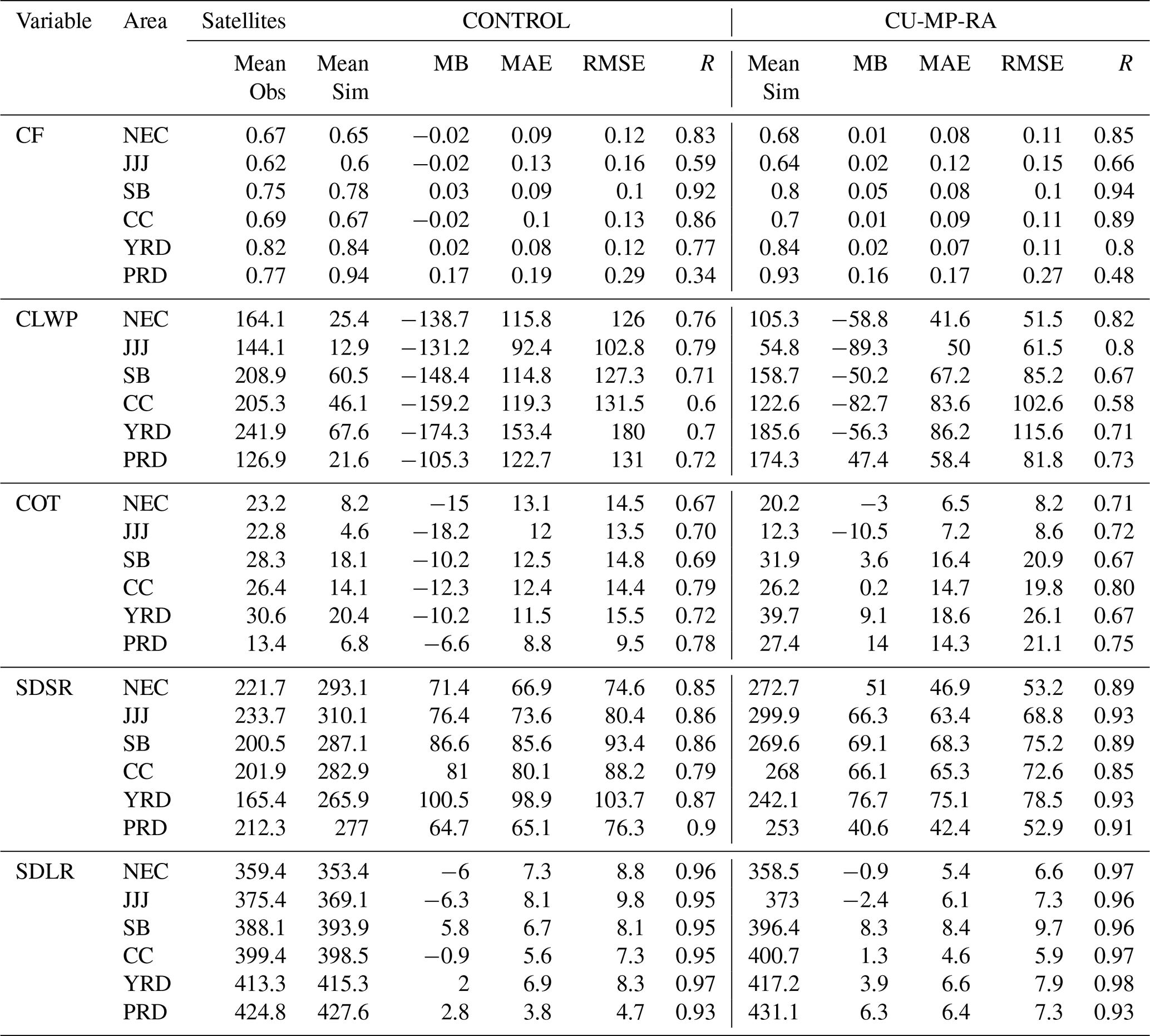
Figure 5 compares the time-averaged cloud properties in June 2016 between simulations and the VIIRS data. For a comparative evaluation, the model simulations are sampled according to transit times of satellites over China. The transit time of VIIRS over China occurs between approximately 13:00 and 14:00 local time, and the corresponding simulations for comparison are averaged hourly data at 13:00 and 14:00 local time. From the VIIRS data, CF, CLWP, and COT all show a distribution of high values in the south and low values in the north in June 2016 in central and eastern China, mainly related to the higher RH in the south. Both the CONTROL and CU-MP-RA experiments reproduce the spatial distribution of cloud properties, but the simulated CF, CLWP, and COT all have some bias in terms of magnitude, and the specific statistics (MB, mean absolute error (MAE), root-mean-square error (RMSE), and correlation coefficient (R)) can be seen in Table 4. For total CF, the model performs better in the north but shows a significant overestimation in the south (e.g., the MB values of total CF in the PRD for the CONTROL and CU-MP-RA experiments reach 0.17 and 0.16, respectively), which is mainly related to the overestimation of high CF in the south (figure omitted). Compared to the CONTROL experiment, the middle and low CF almost all increase throughout central and eastern China, with a maximum value of more than 0.38 and 0.25, while high CF decreases in most areas in the CU-MP-RA experiment (Fig. S1 in the Supplement). The CONTROL experiment also significantly underestimated the CLWP (COT) over the whole domain, where the MB values in the NEC, JJJ, SC, CC, YRD, and PRD regions are −138.7 (−15), −131.2 (−18.2), −148.4 (−10.2), −159.2 (−12.3), −174.3 (−10.2), and −105.3 (−6.6) g m⁻². Compared to the CONTROL experiment, CU-MP-RA shows significantly increased CLWP, especially in the southern regions of China (e.g., the YRD), where convection occurs more frequently and where water vapor conditions are better. In addition, the coverage of cloud water in the model, coupled with subgrid-scale cloud microphysics and radiation feedback, is larger and contains some areas that are not saturated with respect to water at the grid scale. Correspondingly, the MB values of CLWP (COT) in the NEC, JJJ, SC, CC, YRD, and PRD regions for the CU-MP-RA experiment are −58.8 (−3), −89.3 (−10.5), −50.2 (3.6), −82.7 (0.2), −56.3 (9.1), and 47.4 (14) g m⁻², respectively. It can be seen that the CU-MP-RA experiment generally improves the underestimated CLWP in these six regions (especially in the YRD), resulting in a 55.1 % decrease (from 142.9 to 64.1 g m⁻²) in the overall MB averaged over the six regions, which is closer to the VIIRS data. Slightly differently from CLWP, CU-MP-RA does not generally show a decrease in the MB of COT in each region (e.g., the absolute MB of COT in the PRD increases by 7.4), which suggests that the impact of subgrid-scale cloud microphysics and radiation feedback on the accuracy of NWP also depends on the local errors of the model itself. Even if the subgrid-scale cloud microphysics and radiation feedback are considered in the model, the simulations of cloud properties still have some bias. The problem of poorly simulated cloud properties is relatively common in both global and regional NWP models (Lauer and Hamilton, 2013; Wang et al., 2021; Glotfelty et al., 2019), which is one of the key issues that need to be urgently solved in the current scientific community. Overall, the CU-MP-RA experiment shows relatively better performance compared to the CONTROL experiment in June 2016 in central and eastern China for cloud properties.

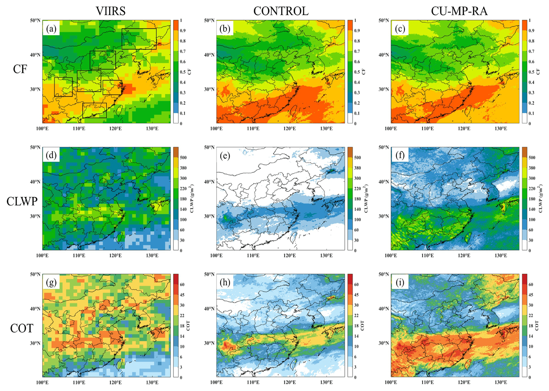
Figure 5 The spatial distribution of time-averaged (a–c) CF, (d–f) CLWP, and (g–i) COT in June 2016. Panels (a, d, g), (b, e, h), and (c, f, i) show the VIIRS, CONTROL, and CU-MP-RA experiments, respectively.

Table 4 Statistics of simulated CF, CLWP (g m⁻²), COT, SDSR (W m⁻²), and SDLR (W m⁻²) for the CONTROL and CU-MP-RA experiments.

5.2.2 Radiation properties

Figure 6 compares the time average radiation properties in June 2016 between the simulations and CERES data. The corresponding simulations for comparison with CERES data are 24 h averaged values. Influenced by cloud characteristics, the SDSR in June 2016 shows a distribution of low values in the south and high values in the north, respectively, while the opposite is true for the SDLR. The CONTROL and CU-MP-RA experiments can reproduce the spatial distribution of the radiative properties. For SDLR, this model has a good prediction performance. This is supported by relevant statistical indicators (Table 4). Compared to the CONTROL experiment, the CU-MP-RA experiment improves the underestimation of SDLR in the northern part of the domain (e.g., the MB of SDLR decreases from −6 and −6.3 W m⁻² to −0.9 and −2.4 W m⁻² in the NEC and JJJ regions, respectively) but further overestimates the SDLR in most of the southern regions (e.g., the MB increases from 2 and 2.8 W m⁻² to 3.9 and 6.3 W m⁻² in the YRD and PRD, respectively). For SDSR, there are significant overestimations for both the CONTROL and CU-MP-RA experiments (e.g., the MB values reach up to 100.5 and 76.7 W m⁻² in the YRD), which may be related to the poor performance in terms of the simulation of cloud properties by the commonly reported mesoscale NWP models (Lauer and Hamilton, 2013; Wang et al., 2021). Compared with the two experiments, the CU-MP-RA experiment improved the overestimation of SDSR in the CONTROL experiment to a certain extent, especially in the regions where CLWP and COT increase significantly (e.g., the YRD and PRD). Correspondingly, the MB of the simulated SDSR averaged over the six regions decreases by ∼ 23.1 % (from 80.1 to 61.6 W m⁻²). Here, we further compare the prediction performance of the CONTROL and CU-MP-RA experiments for SDSR with hour-by-hour ground-based observations (Fig. 7). Similarly to the results of the two experiments compared with the CERES data, the daytime SDSR simulated by the CU-MP-RA experiment is closer to the observations than that of the CONTROL experiment in general, with the MB in the NEC, JJJ, SC, CC, YRD, and PRD regions decreasing by 30.5, 16.1, 29.6, 23.2, 40.5, and 41.2 W m⁻². The decrease in the upper quartile of SDSR bias is larger than that in the lower quartile in all six typical regions. The larger SDSR bias tends to appear in the midday to mid-afternoon period, which indicates that the improvement in the SDSR bias induced by the subgrid-scale cloud microphysics and radiation feedback is mainly manifested in the midday to mid-afternoon period.

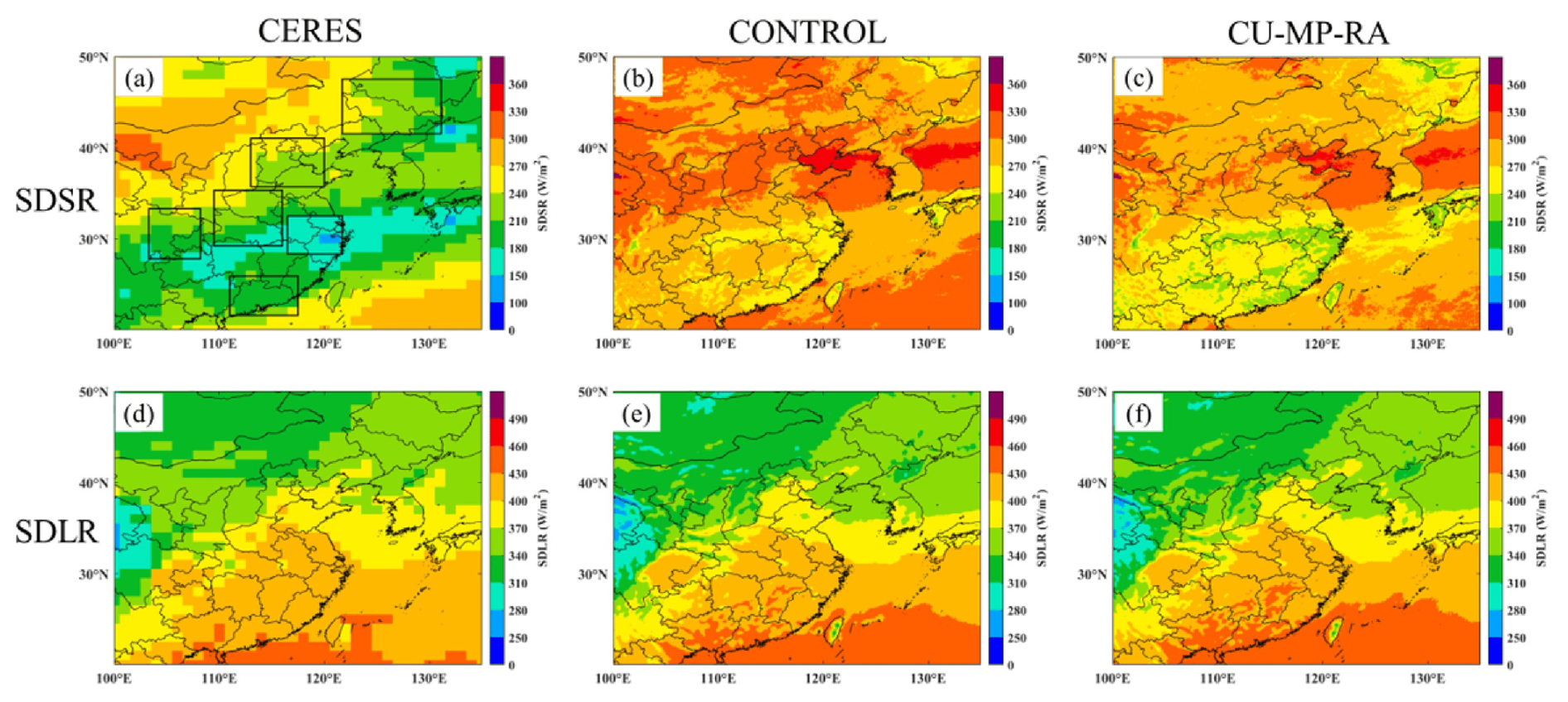
Figure 6 The spatial distribution of time-averaged (a–c) SDSR and (d–f) SDLR in June 2016. Panels (a, d), (b, e), and (c, f) show the CERES, CONTROL, and CU-MP-RA experiments, respectively.

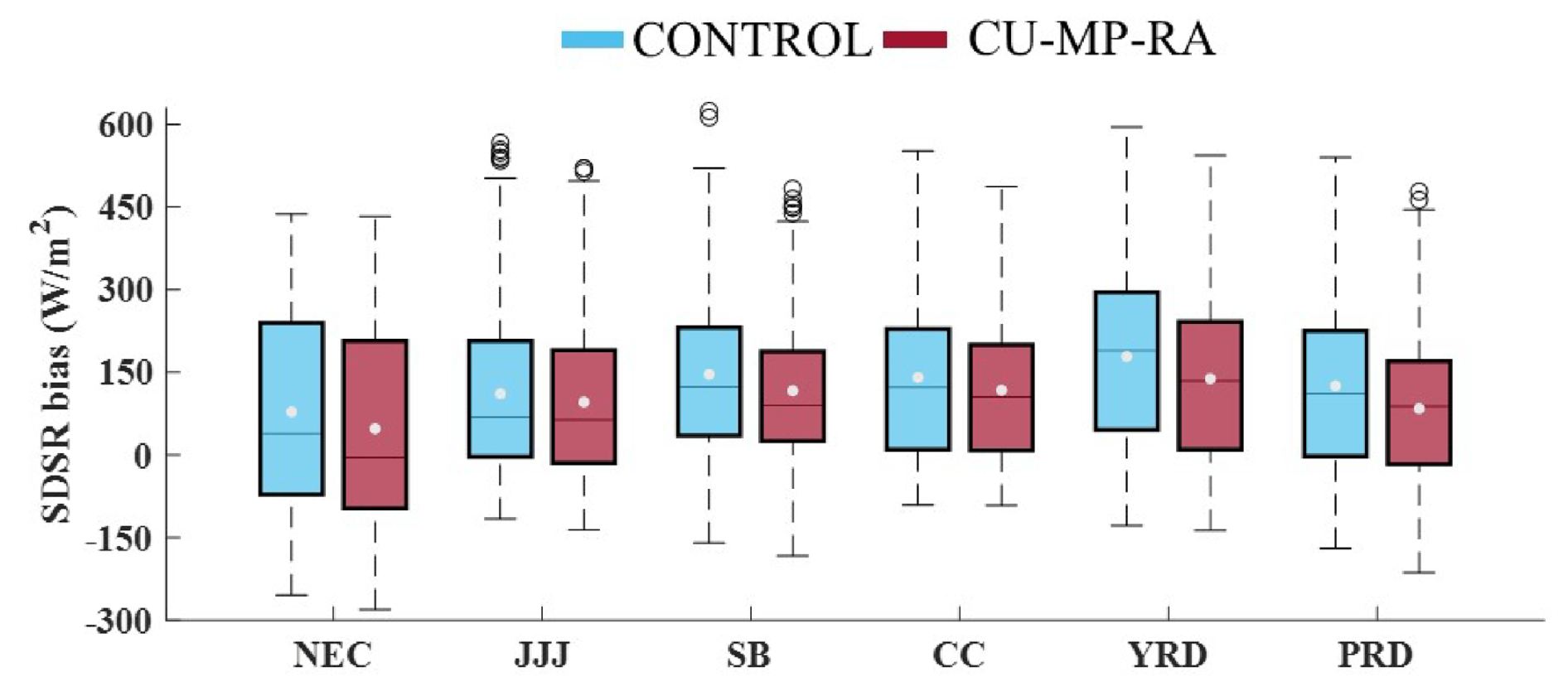
Figure 7 Regional average bias of simulated daytime SDSR in the NEC, JJJ, SB, CC, YRD, and PRD regions during the study period. The interquartile range is shown by boxes and with whiskers for the most extreme data points, excluding outliers. The central lines and white dots present the median and mean values, respectively. The blue and red boxes are the values from the CONTROL and CU-MP-RA experiments, respectively.

5.2.3 Temperature

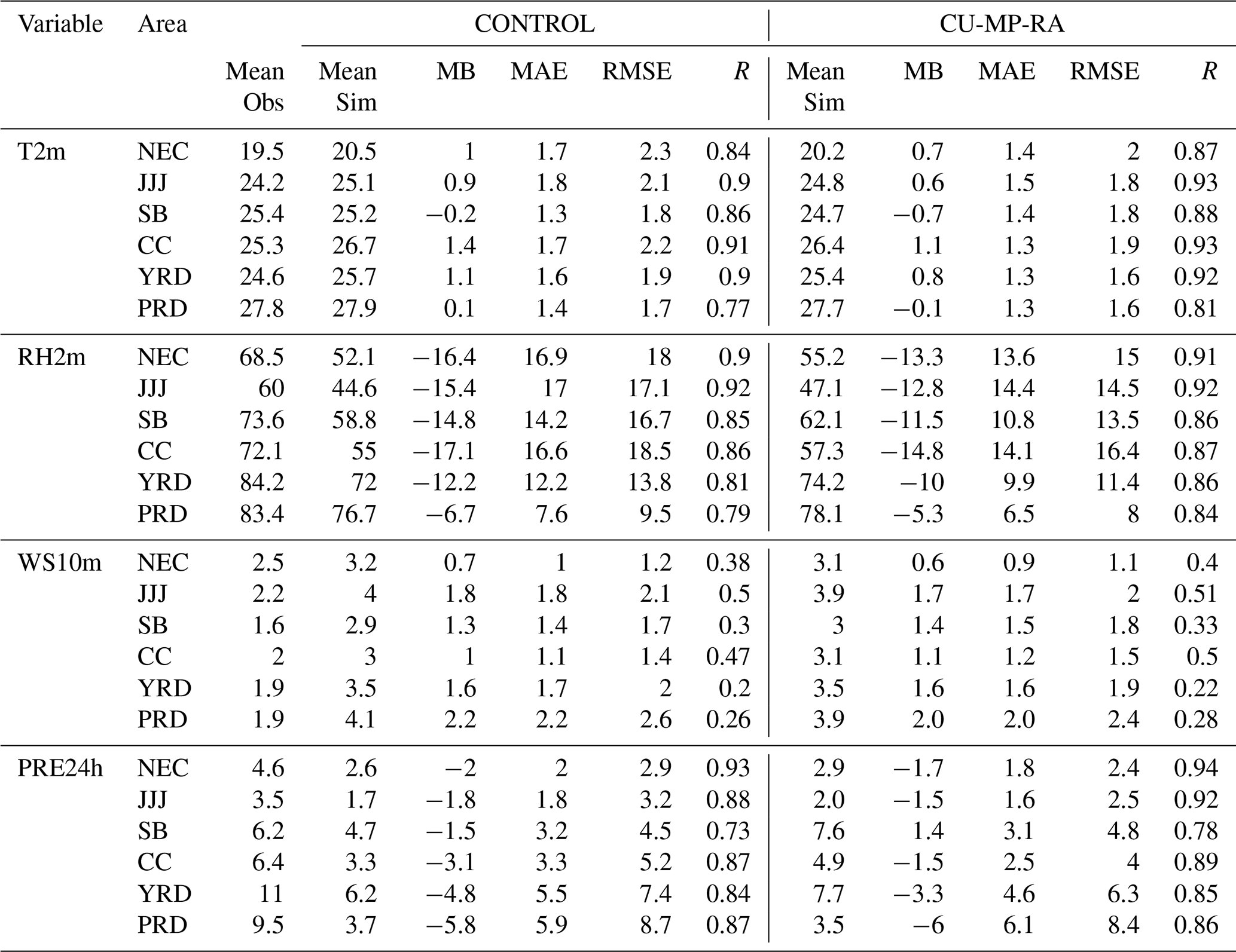
Figure 8 shows the comparisons of the observed and simulated temperatures. For T2m, this model has a better performance overall, and the related statistical indicators (Table 5) also show that the model's simulation performance is in the middle compared with other studies or models (Bozzo et al., 2020; Wang et al., 2021; Gao et al., 2022). Compared with observations, both the CONTROL and CU-MP-RA experiments significantly overestimate T2m in most plains and underestimate T2m in some mountainous areas, thus overestimating terrestrial T2m in the domain as a whole. Unlike other mesoscale NWP models that usually exhibit overall negative regional MB values for T2m in summer, the overall positive MB in the CMA_Meso5.1/CUACE model may be related to the underestimated aerosol concentration, the selection of boundary layer schemes, etc. (Xie et al., 2012). The T2m in the CU-MP-RA experiment is smaller than that in the CONTROL experiment due to the increase in COT and the decrease in SDSR caused by the subgrid-scale cloud microphysics and radiation feedback, which, correspondingly, reduces the positive MB of T2m in the vast majority of regions, with the MB of T2m averaged over the six regions decreasing by ∼ 40 % (from 0.75 to 0.4 °C). Other statistical indicators also show the improved performance of T2m simulations in the CU-MP-RA experiment (Table 5). However, for the SB region, with a large negative MB value for T2m, the cooling effect of subgrid-scale cloud microphysics and radiation feedback leads to a further increase in the negative MB (from −0.2 to −0.7 °C), but the T2m correlation coefficients increase in this region. Also, this model reproduces the vertical profile of temperature better, but the six typical regions generally have a significant positive MB below about 900 hPa (Fig. 8f). Temperature over most of the air layers as simulated by the CU-MP-RA experiment is closer to observations than that of the CONTROL experiment, with the ranges of the mean absolute error skill score (MAESS) of temperatures from 2 m to 500 hPa in the NEC, JJJ, SC, CC, YRD, and PRD regions being −2 % to 17 %, 5 % to 0.22 %, 3 % to 25 %, −8 % to 22 %, 1 % to 33 %, and 5 % to 32 % (Fig. 11).

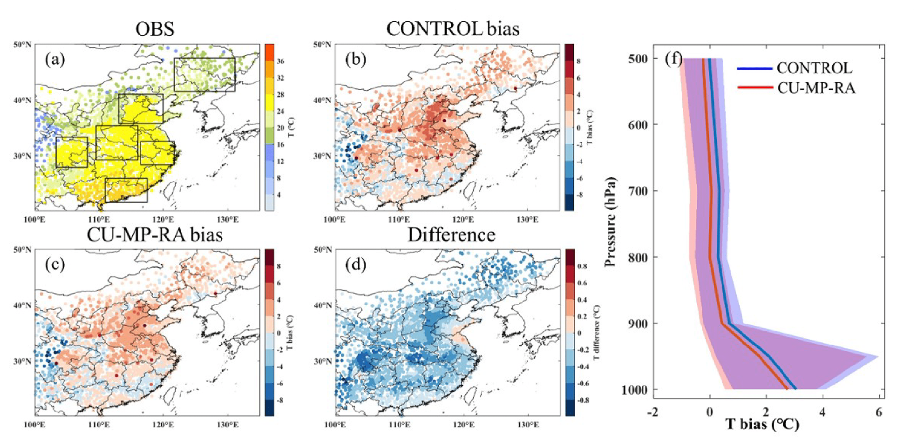
Figure 8 The spatial distribution of time-averaged T2m and the vertical profiles of MB values of temperature in June 2016. (a) The observations. (b) The MB of T2m in the CONTROL experiment. (c) The MB of T2m in the CU-MP-RA experiment. (c) The difference in terms of T2m between the CU-MP-RA and CONTROL experiments. (f) The vertical profiles of the MB of temperature in the CONTROL and CU-MP-RA experiments. In (f), the shading represents the spread of the MB of temperature in six regions, and the solid lines are their average results.

Table 5 Statistics of simulated T2m (°C), RH2m (%), WS10m (m s⁻¹), and 24 h cumulative precipitation (PRE24h, mm) for the CONTROL and CU-MP-RA experiments.

5.2.4 RH

Figure 9 shows the comparisons of observed and simulated RH. The spatial distribution of the MB of RH2m is influenced by the MB of T2m (the larger positive MB of T2m corresponds to the larger negative MB of RH2m), mainly because the calculation of RH is temperature dependent. For example, compared between these six regions, the MB of T2m in the CC region (1.4 and 1.1 °C for the CONTROL and CU-MP-RA experiments, respectively) is the largest, and, thus, the MB of RH2m (−17.1 % and −14.8 % for the CONTROL and CU-MP-RA experiments, respectively) is also the largest (Table 5). Compared between these two experiments, the CU-MP-RA experiment generally has a smaller MB of RH2m over this study area, with an overall ∼ 18.1 % (relative change) decrease in MB averaged over the six regions (from −13.8 % to −11.3 %) and an improvement in all other statistical indicators (Table 5), suggesting a better performance of the CU-MP-RA experiment in terms of RH2m predictions. For the vertical profile of RH, both the CONTROL and CU-MP-RA experiments have a negative MB of RH below ∼ 900 hPa and a positive MB above ∼ 900 hPa in most areas (Fig. 9f). Due to the humidity-raising effects of the subgrid-scale cloud microphysics and radiation feedback, the CU-MP-RA experiment generally shows a better performance than the CONTROL experiment for RH at 1000–900 hPa in the study area, where the MAESS ranges of RH from 1000 to 900 hPa in the NEC, JJJ, CC, YRD, and PRD regions are 1 % to 21 %, 5 % to 14 %, 0.1 % to 0.17 %, 2 % to 15 %, and 7 % to 13 %, respectively (Fig. 11). A worsened performance of the RH simulation occurs in all air layers in the SB and above ∼ 900 hPa in other regions due to an increase in the positive MB of the RH to some extent, suggesting that the impact of subgrid-scale cloud microphysics and radiation feedback on RH predictions also relates to the local errors of the model itself.

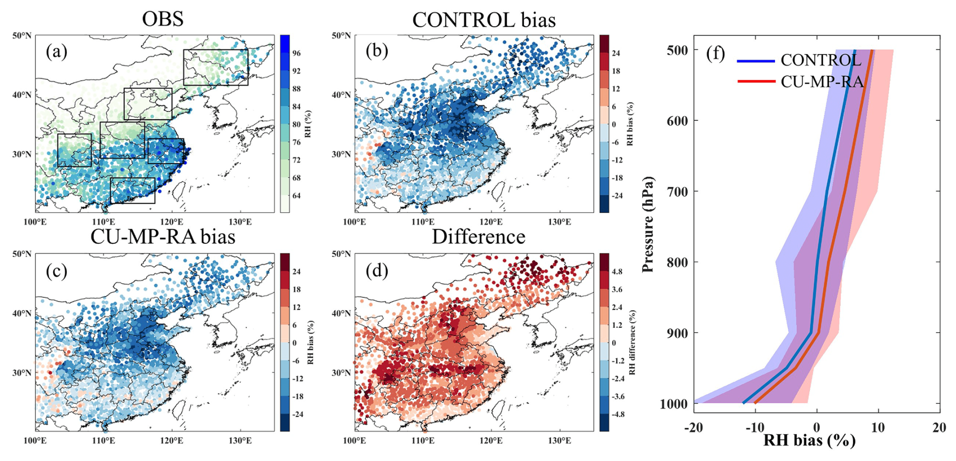
Figure 9 The spatial distribution of time-averaged RH2m and the vertical profiles of the MB of RH in June 2016. (a) The observations. (b) The MB of RH2m in the CONTROL experiment. (c) The MB of RH2m in the CU-MP-RA experiment. (c) The difference in terms of RH2m between the CU-MP-RA and CONTROL experiments. (f) The vertical profiles of the MB of RH in the CONTROL and CU-MP-RA experiments. In (f), the shading represents the spread of the MB of RH in six regions, and the solid lines are their average results.

5.2.5 Wind speed

Figure 10 shows the comparisons of observed and simulated wind speed. The performance of the WS10m simulations compared to observations is comparable to that of other studies and models (Table 5). Both the CONTROL and CU-MP-RA experiments overestimate WS10m over the study area, especially in the PRD, where the MB reaches 2.2 and 1.9 m s⁻¹, respectively. This systematic overestimation of WS10m is a common problem in mesoscale NWP models which is likely to be related to the treatment of the underlying surface in the models (Jimenez and Dudhia, 2012; Jia and Zhang, 2021). For example, the complex underlying surface of the JJJ, YRD, and PRD regions cannot be fully resolved in this model, and the relatively smooth treatment of the underlying surface leads to a significant overestimation of WS10m in these regions (Table 5). Compared with the CONTROL experiment, the WS10m increases or decreases in different regions in the CU-MP-RA experiment and consequently increases or decreases the MB, which leads to an overall less pronounced improvement in the MB of WS10m averaged over the six regions. As can be seen from the other statistical indicators, the correlation coefficients of WS10m simulations for the different regions are somewhat improved (Table 5). Further comparison reveals that the regions with increased WS10m are consistent with the regions with significantly increased CLWP. It is speculated that this may be related to decreased atmospheric stability caused by the more significant cooling in the upper atmosphere in these regions. In contrast, the decrease in WS10m is likely to be associated with the increased atmospheric stability caused by the decline in the near-surface temperature. For the vertical profiles of wind speed, overall, both the CONTROL and CU-MP-RA experiments are in good agreement with observations. However, wind speed is still overestimated in the lower air layers over most regions (Fig. 10f). The comparison of the two experiments shows that the subgrid-scale cloud microphysics and radiation feedback have more complex effects on the vertical profile of wind speed than temperature or humidity, resulting in an overall decrease in wind speed below ∼ 800 hPa and an increase in wind speed above ∼ 800 hPa. The MAESS values of wind speed from 10 m to 500 hPa are also greater than 0 in most regions, reflecting the improvement in terms of subgrid-scale cloud microphysics and radiation feedback on the vertical profile of wind speed. It is worth noting that this improvement varies significantly among different regions. For example, the MAESS values over most air layers in the YRD and PRD are considerably larger than those in several other regions (Fig. 11), which may be related to the cloud water content and local errors of the model itself.

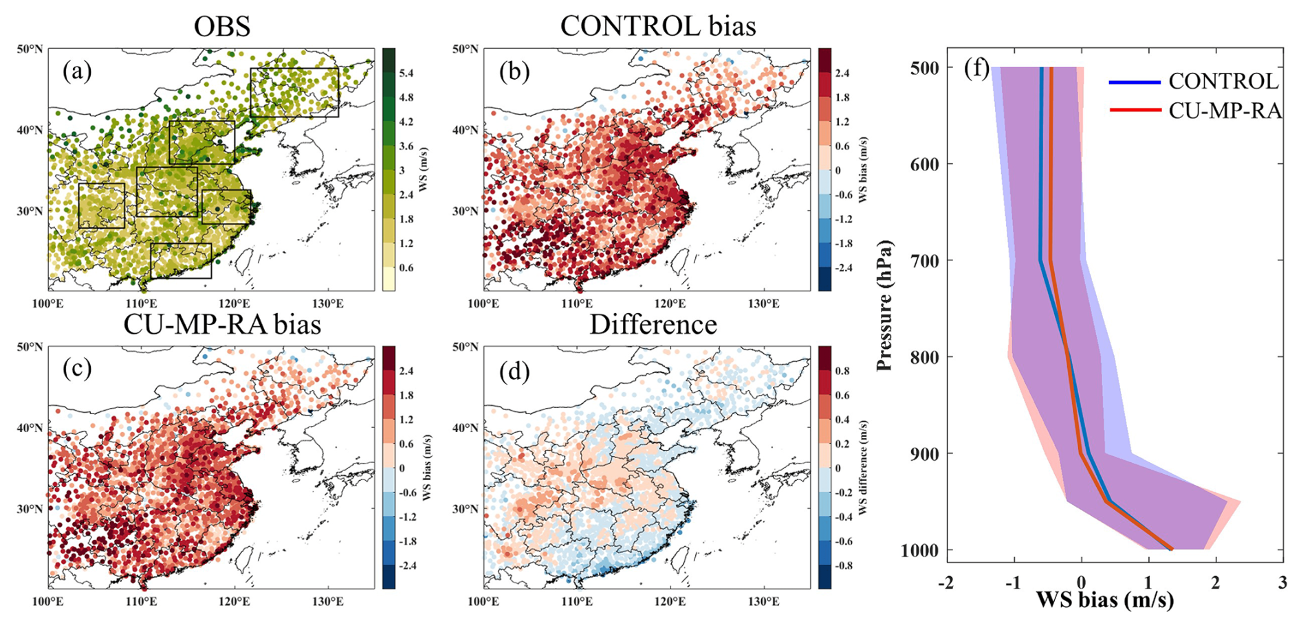
Figure 10 The spatial distribution of time-averaged WS10m and the vertical profiles of the MB of wind speed in June 2016. (a) The observations. (b) The MB of WS10m in the CONTROL experiment. (c) The MB of WS10m in the CU-MP-RA experiment. (c) The difference in terms of WS10m between the CU-MP-RA and CONTROL experiments. (f) The vertical profiles of the MB of wind speed in the CONTROL and CU-MP-RA experiments. In (f), the shading is the spread of the MB of wind speed in six regions, and the solid lines are their average results.

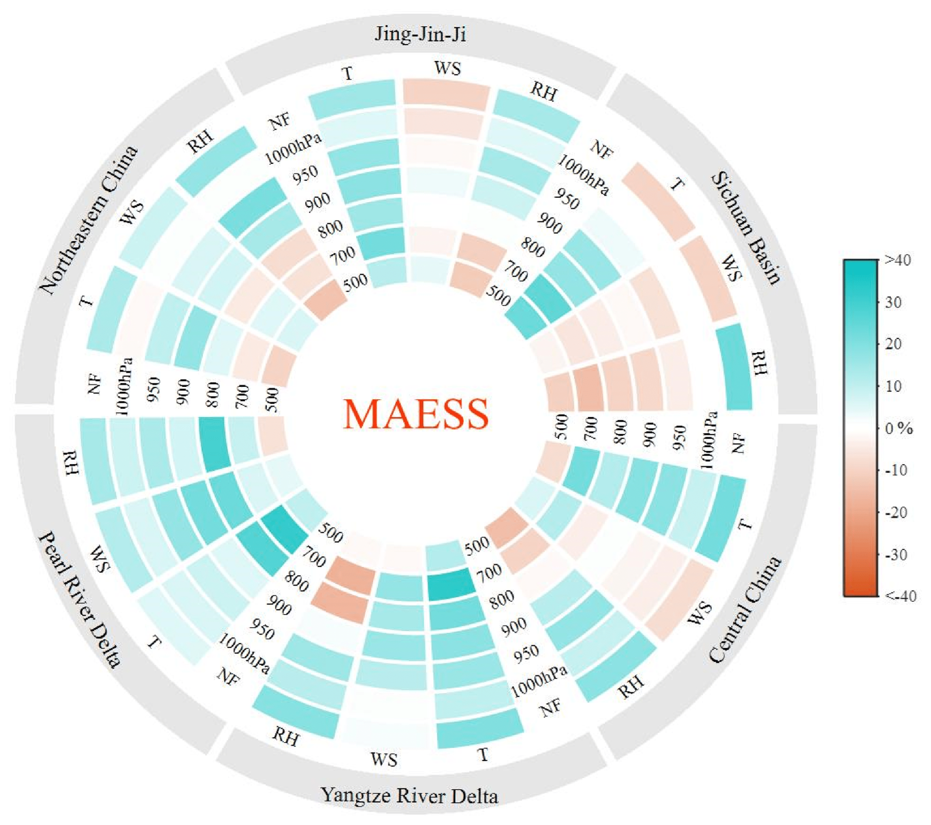
Figure 11 Hourly MAESS (× $\mathrm{MAESS}=\left(\mathrm{1}-\frac{{\mathrm{MAE}}_{\mathrm{ARI}}}{{\mathrm{MAE}}_{\text{NO-ARI}}}\right)\mathrm{100}\mathrm{\%}$, where MAE_ARI and MAE_NO-ARI represent the mean absolute error (MAE) (MAE=|mean bias|)) of predicted meteorological factors from the CU-MP-RA and CONTROL experiments in six regions (NEC, JJJ, SB, CC, YRD, and PRD). The green-filled (red-filled) boxes represent the subgrid-scale ACI with positive (negative) effects.

5.2.6 Precipitation

Figure 12 shows the comparisons of observed and simulated precipitation. Compared with observations, both the CONTROL and CU-MP-RA experiments reproduce the overall spatial distribution of summer precipitation in central and eastern China, with more precipitation in the south and less precipitation in the north. The values of related statistical indicators (Table 5) also show that the simulation performance of precipitation is similar to that of other NWP models (e.g., WRF-CMAQ, WRF) or compared to results reported in previous studies (Glotfelty et al., 2019; Wang et al., 2021; Wong et al., 2012). The precipitation in central and eastern China is significantly underestimated in the CONTROL experiment, in which the MB of 24 h cumulative precipitation in the NEC, JJJ, SC, CC, YRD, and PRD regions is −2, −1.8, −1.5, −3.1, −4.8, and −5.8 mm, respectively. Compared with the CONTROL experiment, the 24 h cumulative precipitation in the CU-MP-RA experiment increases due to the significant enhancement of precipitation at the grid scale (Fig. S2), which leads to an improvement in the underestimation of precipitation in the majority of regions, where the MB of 24 h cumulative precipitation in the NEC, JJJ, SC, CC, YRD, and PRD regions is −1.7, −1.5, 1.4, −1.5, −3.3, and −6 mm, respectively. Overall, the MB of 24 h cumulative precipitation averaged over six regions decreased by ∼ 34.4 % (from −3.2 to −2.1 mm). The increases in precipitation is accompanied by increases in water vapor and grid-scale cloud water or ice (Figs. S3 and S4), associated with the redistribution of water vapor and convective detrainment of cloud water or ice (Song and Zhang, 2011). Other relevant statistical indicators also show the improvement in 24 h cumulative precipitation in the NEC, JJJ, SC, CC, and YRD regions (Table 5). It is worth noting that the MB of precipitation in the PRD increases due to a slight decrease in precipitation, which is speculated to be related to the competition for water vapor among different regions (Glotfelty et al., 2020).

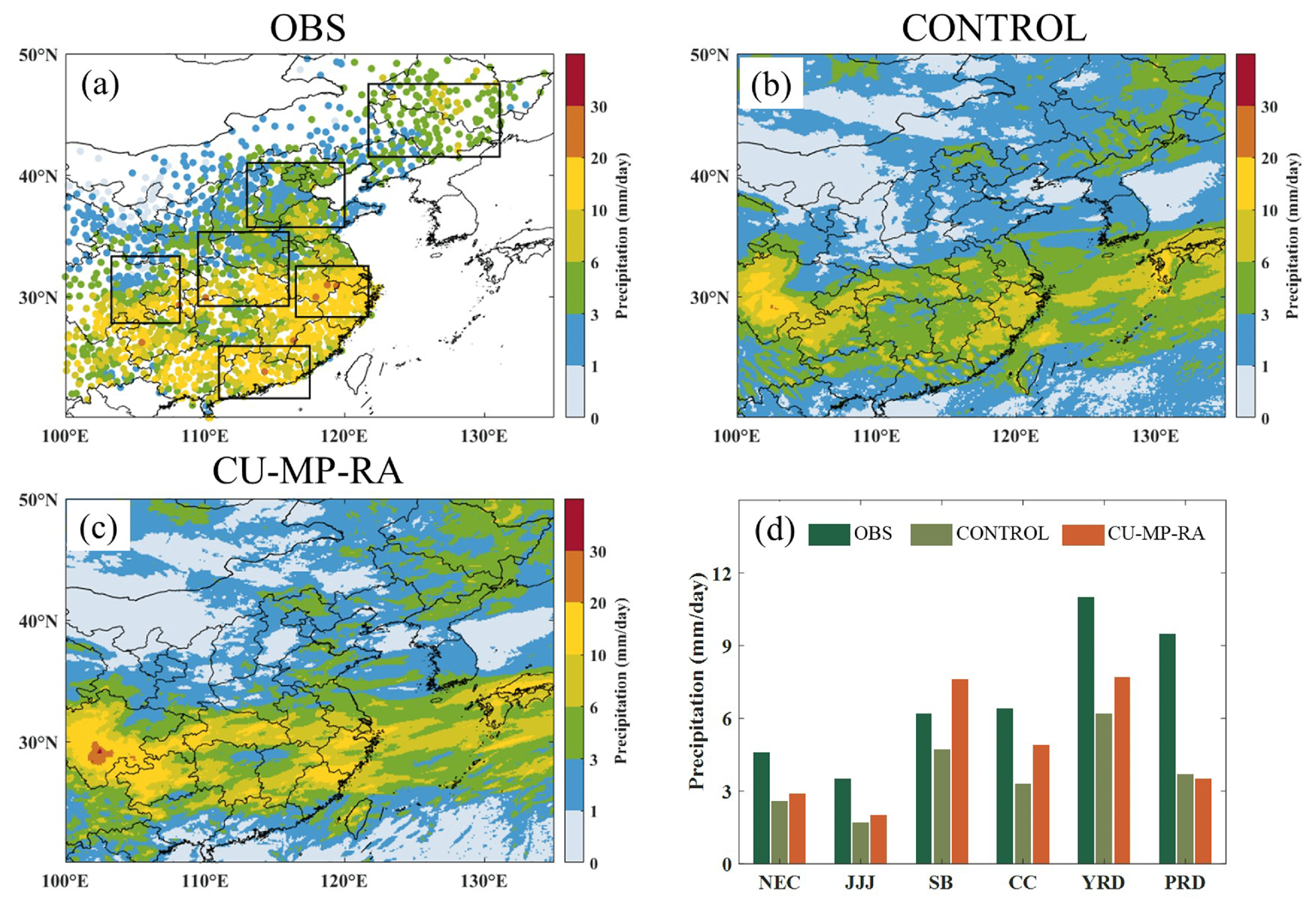
Figure 12 The spatial distribution of time-averaged 24 h cumulative precipitation in June 2016 from the (a) observations, (b) CONTROL experiment, and (c) CU-MP-RA experiment. (d) The comparison of time-averaged 24 h cumulative precipitation in different regions.

5.3 Impact of anthropogenic aerosol on typical deep-convective precipitation prediction via subgrid-scale ACI

The discussion in the previous sections has shown that considering ACI at the subgrid scale in this model improves the performance of most predicted meteorological factors. In this section, the model coupled with subgrid-scale ACI is utilized to separately explore the effects of anthropogenic aerosol perturbations at the subgrid scale by controlling anthropogenic aerosol emissions for a typical deep-convective precipitation event.

The individual case chosen for the study is a continuous heavy-precipitation event from 26 to 29 June 2016 in the YRD. During this period, the YRD region was influenced by a deep-convective cloud system (Fig. 13), with the regionally averaged cumulative precipitation approaching 90 mm (Fig. 15a, b); the model can reproduce the precipitation event (Fig. 15c). As shown in Fig. 13, on 26 June 2016, a convective cloud with high cloud top pressure and low cloud top height was over the YRD. On 27 and 28 June 2016, the cloud top pressure decreased, and cloud top height rose, conditions which are conducive to water vapor condensation and precipitation production. As a result, the 24 h cumulative precipitation exceeded 50 mm at most stations during this period. On 29 June 2016, the convective cloud over this region gradually dissipated, accompanied by a decrease in precipitation. On 30 June 2016, the convective cloud completely dissipated. In addition, as shown in Fig. 14, the overall aerosol levels in the YRD were relatively low between 26 and 29 June 2016, with the peak in PM_2.5 mass concentrations being less than 40 µg m⁻³.

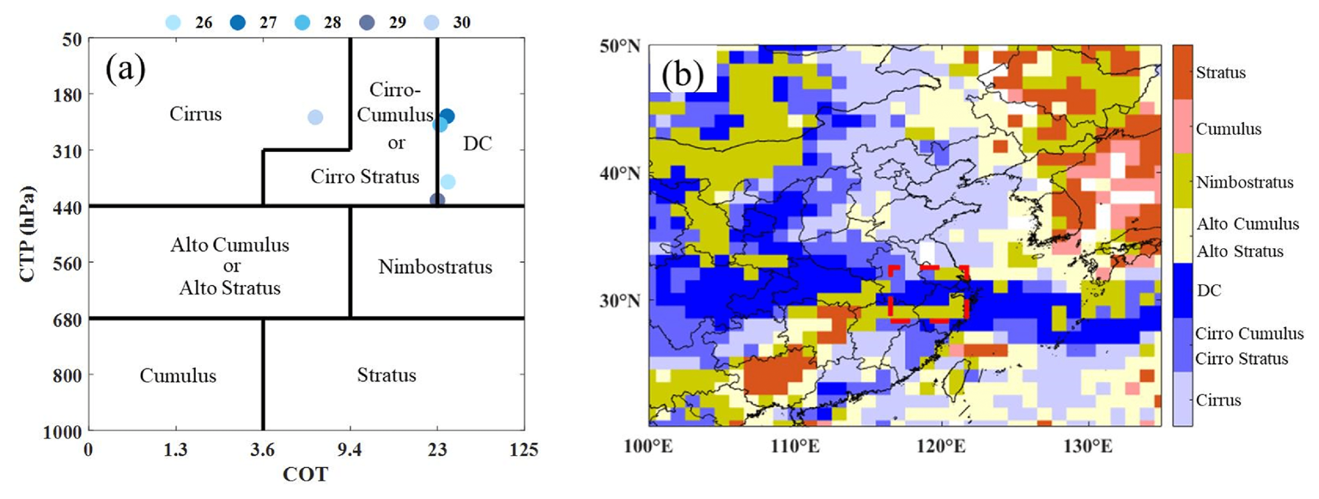
Figure 13 (a) Cloud types over the YRD from 26 to 30 June 2016 based on the International Satellite Cloud Climatology Project (ISCCP) cloud classification algorithm (Hahn et al., 2001). (b) The spatial distribution of cloud types in central and eastern China on 28 June 2016. The dashed red rectangle is the location of the YRD region.

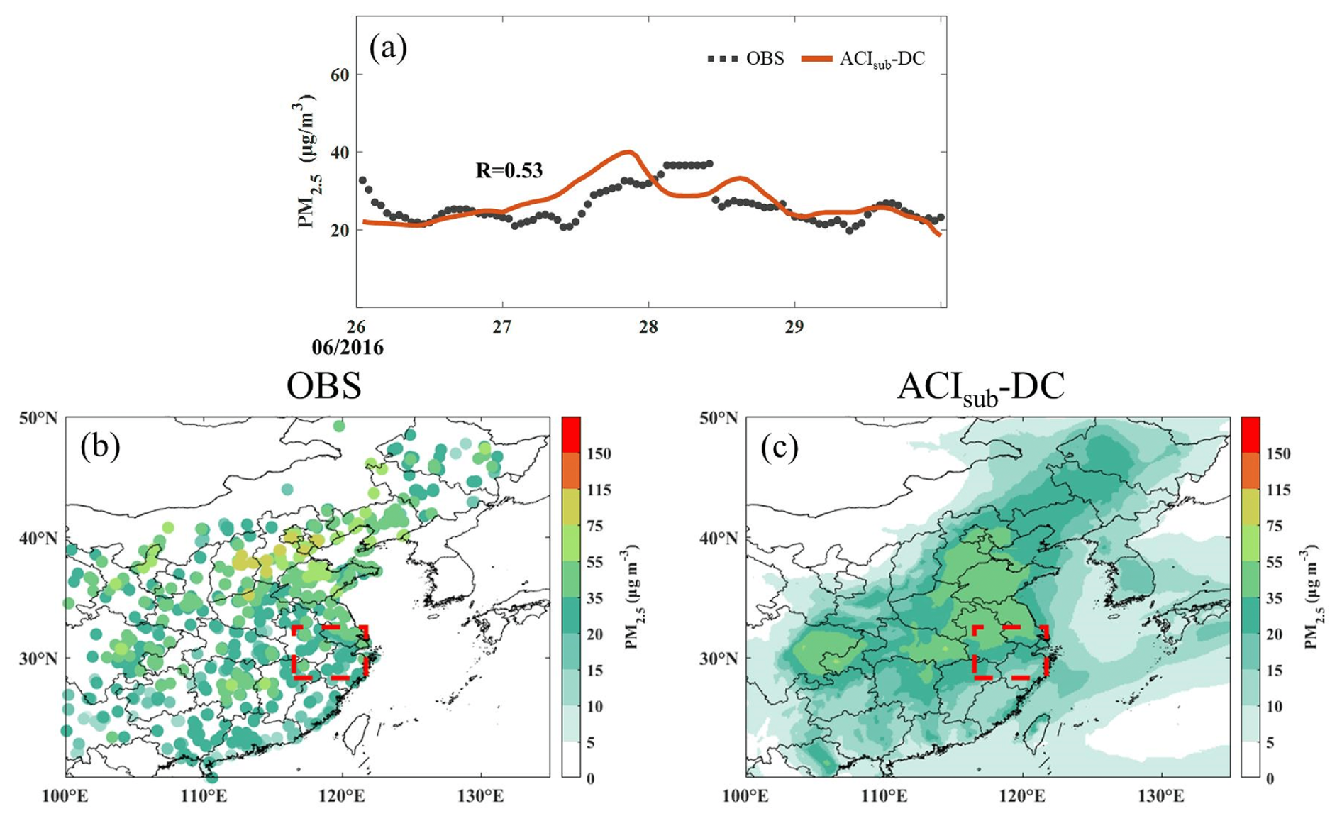
Figure 14 (a) The temporal variation in the regional average PM_2.5 mass concentration in the YRD. The spatial distribution of the (b) observations and (c) simulations by the ACI_sub-DC experiment of the time-averaged PM_2.5 mass concentration from 26 to 29 June 2016.

Figure 15d shows the observed and simulated temporal variations in the regional average hourly precipitation in the YRD. It can be seen that the simulations in both experiments are in good agreement with the observations, capturing both the rising and falling periods of precipitation, with R exceeding 0.7 (Fig. 15e). The comparison of the ACI_sub-DC and CACI_sub-DC experiments shows that anthropogenic aerosol leads to a decrease in regional average precipitation in the YRD via subgrid-scale ACI, with a ∼ 5.6 % decrease (from 82 to 77.6 mm) in cumulative precipitation for the study period. Compared with the CACI_sub-DC experiment, the ACI_sub-DC experiment shows a better performance in simulating this heavy-precipitation event over the YRD, with the centered root-mean-square discrepancy (CRMSD) decreasing from 0.63 to 0.56 and the standard deviation (SD) decreasing from 0.89 to 0.84 (Fig. 15e).

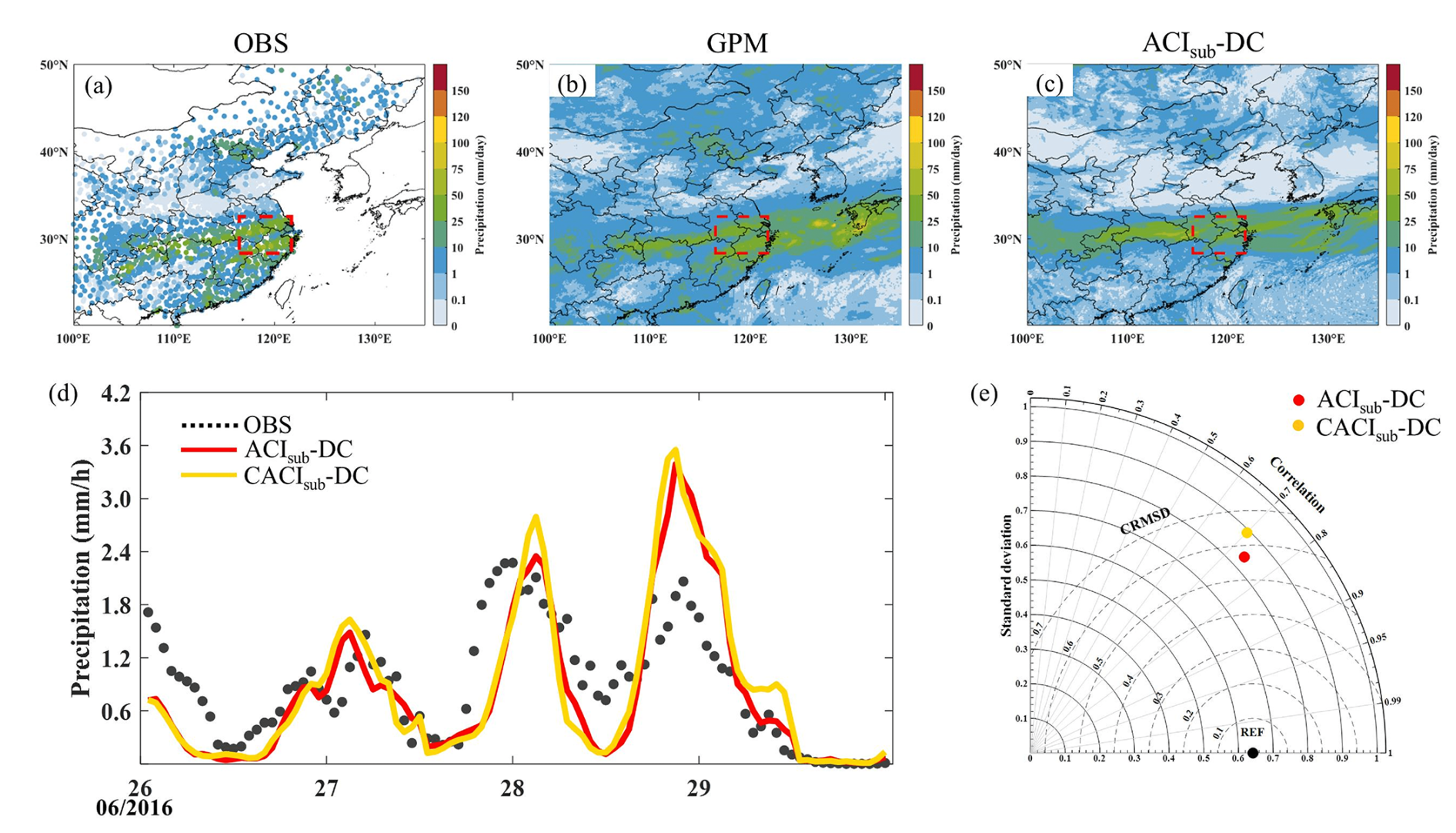
Figure 15 The spatial distribution of time-averaged 24 h cumulative precipitation from 26 to 29 June 2016 in the (a) observations, (b) GPM, and (c) ACI_sub-DC experiment. The (d) time variation and (e) Taylor diagram of observed and simulated regional average hourly precipitation in the YRD from 26 to 29 June. In the Taylor diagram, the REF is the observation, the vertical coordinate is the standard deviation (SD), the distance between the simulations and REF is the centered root-mean-square deviation (CRMSD), and the position of the azimuth is the correlation coefficient (R).

Further detailed analyses are carried out to investigate the causes of precipitation changes. Compared with the CACI_sub-DC experiment, the anthropogenic aerosol emissions in the ACI_sub-DC experiment lead to an increase of 23.5 µg m⁻³ in the average PM_2.5 mass concentration in the YRD during the study period (Fig. 16a), which directly causes the regional average cloud droplet number concentration of convective cloud at the subgrid scale (averaged over 1–6 km) to increase by about 3.2 × 10⁶ m⁻³ (Fig. 16b). Notably, the decreased cloud droplet number concentration within some YRD regions may be related to lower environmental supersaturation due to thermodynamic and/or dynamic perturbations (e.g., weaker updrafts, evaporative cooling) (Fan et al., 2016; Glotfelty et al., 2020). Anthropogenic aerosol directly induces the changes in cloud droplet number concentration at the subgrid scale, further influencing precipitation. The simulated precipitation is categorized into subgrid-scale precipitation from the cumulus convection scheme and grid-scale precipitation from the cloud microphysics scheme, and these two types of precipitation are studied separately. As can be seen in Fig. 17a and c, the anthropogenic aerosol leads to a decrease in precipitation at both the subgrid scale and grid scale via subgrid-scale ACI, with the total cumulative precipitation during the study period decreasing by 2.9 % (from 9.43 to 9.16 mm) and 5.9 % (from 72.8 to 68.5 mm), respectively.

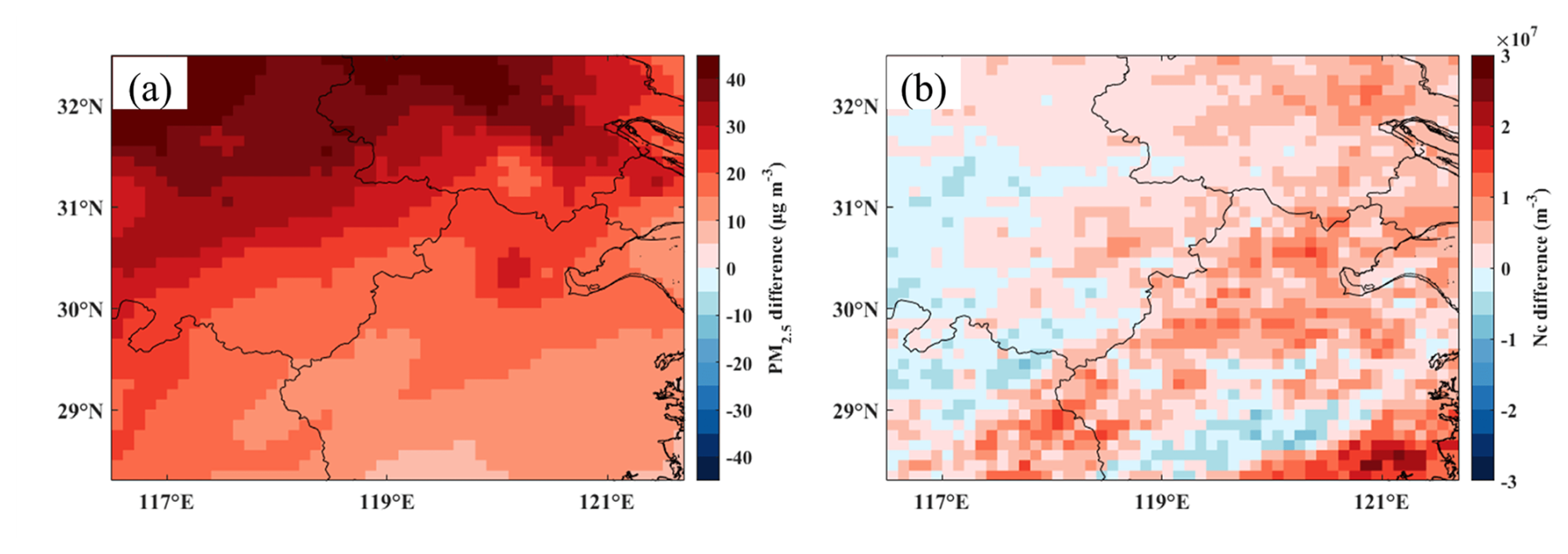
Figure 16 The spatial distribution of the difference between the ACI_sub-DC and CACI_sub-DC experiments for the time-averaged (a) PM_2.5 mass concentration and (b) subgrid-scale cloud droplet number concentration (mean values for 1–6 km) from 26 to 29 June 2016.

The decrease in precipitation at the subgrid scale is mainly related to the weaker autoconversion of cloud water to rain at the subgrid scale. As shown in Fig. 17b, it can be seen that there is a general increase in Qc (up to a maximum of 0.06 g kg⁻¹) at the subgrid scale in the ACI_sub-DC experiment compared to in the CACI_sub-DC experiment. At the same time, the anthropogenic aerosol leads to the changes in Qc and the radius of cloud droplets at the subgrid scale in the vertical direction, showing a clear opposite trend (Fig. 18a). Based on this, it is reasonable to conclude that anthropogenic aerosol leads to more but smaller cloud droplets, which is unfavorable for the growth of cloud droplets into raindrops and inhibits the autoconversion process from cloud water to rainwater, thus leading to the increase in cloud water content and the decrease in precipitation at the subgrid scale. The combination of the location of the 0 °C isotherm (a higher proportion of warm region in cloud) and the increase in Qi (which usually leads to an increase in precipitation in the mixed-phase cloud dominated by cold cloud processes) roughly excludes the fact that anthropogenic aerosol leads to a decrease in precipitation at the subgrid scale by influencing cold cloud processes (Ma et al., 2015; Luo et al., 2023; Fan et al., 2016), which remains to be further analyzed in detail for precipitation sources and sinks.

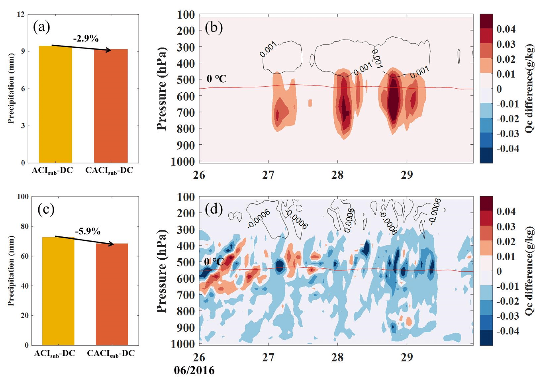
Figure 17 The (a, b) subgrid-scale and (c, d) grid-scale (a, c) cumulative precipitation from 26 to 29 June 2016 and vertical distributions of (b, d) the difference between the ACI_sub-DC and CACI_sub-DC experiments for the regional average Qc and Qi. In (b) and (d), the shading is Qc, the contour is Qi, and the red line is the 0 °C isotherm.

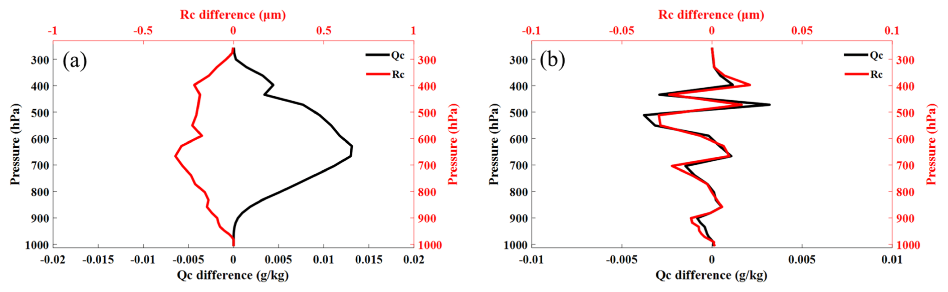
Figure 18 (a) The difference in terms of subgrid-scale Qc and Rc in the YRD between the ACI_sub-DC and CACI_sub-DC experiments. (b) The difference in terms of grid-scale Qc and Rc in the YRD between the ACI_sub-DC and CACI_sub-DC experiments.

The decrease in precipitation at the grid scale is primarily related to the competition of clouds at the subgrid scale for water vapor, resulting in less available water vapor for condensation at the grid scale. As shown in Fig. 17d, Qc at the grid scale decreases (up to a maximum of −0.09 g kg⁻¹) over most air layers during the study period in the ACI_sub-DC experiment compared to in the CACI_sub-DC experiment. In contrast to the changes in the radius of cloud droplets at the subgrid scale, the changed trends in terms of the radius of cloud droplets and Qc at the grid scale in the vertical direction are the same (i.e., the radius of cloud droplets and cloud water content decrease simultaneously) (Fig. 18b). In addition, Qi, Qr, graupel mixing ratio (Qg), and Qs decrease at the grid scale (Fig. 19). These changes lead to a decrease in precipitation at the grid scale. Based on the general reduction in all hydrometeor mixing ratios in cloud and smaller cloud droplets, it is reasonable to assume that this is mainly related to the reduction in water vapor available for condensation at the grid scale. The anthropogenic aerosol–cloud interaction at the subgrid scale is an important reason for the reduction in water vapor at the grid scale. Previous studies have also shown a competing effect on water vapor between subgrid-scale and grid-scale cloud parameterization schemes, which is more pronounced at the subgrid scale (Glotfelty et al., 2019, 2020).

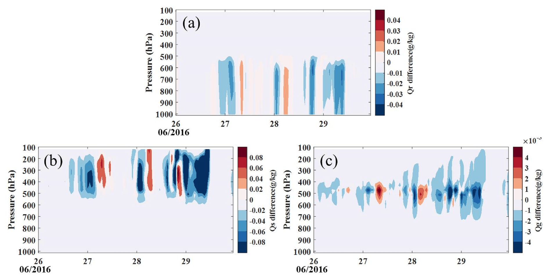
Figure 19 The vertical distribution of the difference between the ACI_sub-DC and CACI_sub-DC experiments for regional average grid-scale (a) Qr, (b) Qs, and (c) Qg in the YRD from 26 to 29 June 2016.

6 Conclusions

In this paper, based on a mesoscale atmospheric chemistry model, CMA_Meso5.1/CUACE, the subgrid-scale ACI mechanism is implemented for convective clouds with horizontal scales smaller than model grid spacing: a double-moment convective cloud microphysical scheme (SZ2011), which explicitly deals with various hydrometeor (cloud water, cloud ice, rain, and snow) microphysical processes of convective clouds, is coupled with the KFeta cumulus convective scheme; the real-time predicted hygroscopic aerosol (OC, SS, SF, NT, and AM) of the CUACE is used to generate cloud droplets at the subgrid scale via the ARG2000 size-resolved activation scheme; the calculated CF, Qc, Qi, Rc, and Ri in the KFeta cumulus convective scheme are transferred to the Goddard shortwave radiation scheme for radiative feedback on the subgrid-scale cloud. Based on reliable PM_2.5 mass and AOD simulations, two sets of experiments are conducted using this updated model. The first set of experiments investigates the performance of the developed model with subgrid-scale cloud microphysics and radiation feedback with regard to the prediction of meteorological factors in summer in different regions (the NEC, JJJ, SC, CC, YRD, and PRD regions) of central and eastern China in terms of whether or not to include the treatment of subgrid-scale cloud microphysics and radiation feedback in the model; the second set of experiments investigates the impact of anthropogenic aerosol on deep-convective precipitation in the YRD via subgrid-scale ACI.

The results show that the coupling of subgrid-scale cloud microphysics with real-time size-resolved hygroscopic aerosol activation and radiation feedback in the model refines cloud representations, e.g., causing underestimated cloud water content and cloud extinction to increase, even in some areas that are not saturated with respect to water at the grid scale. As a result, the attenuation of shortwave radiation is better simulated, with the regional MB of SDSR decreasing by ∼ 23.1 % (∼ 18.5 W m⁻²). The cloud and radiation changes induced by subgrid-scale cloud microphysics and radiation feedback lead to a decrease (∼ 0.35°C) in temperature at 2 m accompanied by an increase (∼ 2.5 %) in RH at 2 m, which helps to reduce the regional MB by ∼ 40 % and ∼ 18.1 %, respectively. This cooling and humidification occur from 1000 to 500 hPa, but the improvement is mainly concentrated in temperature in whole layers and at RH below 900 hPa. Unlike temperature and RH, wind speed increases or decreases at different air layers or regions, possibly relating to changes in atmospheric stability. The treatment of subgrid-scale cloud microphysics and radiation feedback in the model significantly enhances total precipitation further (∼ 1.1 mm), mainly caused by increased precipitation at the grid scale linked to convective detrainment, thus reducing the regional MB of 24 h cumulative precipitation by 34.4 %. Compared with different subregions (the NEC, JJJ, SCB, CC, YRD, and PRD regions) in central and eastern China, the impact of subgrid-scale cloud microphysics and radiation feedback on the prediction of meteorological factors is more significant in the YRD region, which is mainly related to convective conditions and model local errors. In addition, compared with simulations with the anthropogenic emissions turned off, the subgrid-scale actual anthropogenic aerosol emissions cause the grid-scale and subgrid-scale total cumulative precipitation during a typical deep-convective heavy-precipitation event in the YRD to decrease by ∼ 5.6 % (∼ 4.6 mm), which is closer to the observations. It is further found that the decrease in total precipitation is associated with lower autoconversion of cloud water into rain at the subgrid scale and with less water vapor being available for condensation at the grid scale, suggesting a competing effect on water vapor between subgrid-scale and grid-scale cloud.

There is still a need for some complementary work in the future, e.g., systematically distinguishing the differences between subgrid-scale cloud microphysics and radiation feedback effects on meteorological prediction, a study of the differences in terms of the impact of the ACI mechanism on NWP at different grid resolutions (Glotfelty et al., 2020), and the coupling of real-time ice crystal nucleation at the grid scale and subgrid scale and its impacts on the prediction of meteorological factors (Su and Fung, 2018a, b).