Modeling urban pollutant transport at multiple resolutions: impacts of turbulent mixing

Air pollution in cities impacts public health and climate. Turbulent mixing is crucial in pollutant formation and dissipation, yet current atmospheric models struggle to accurately represent it. Turbulent mixing intensity varies with model resolution, which has rarely been analyzed. To investigate turbulent mixing variations at multiple resolutions and their implications for urban pollutant transport, we conducted experiments using the Weather Research and Forecasting model coupled with Chemistry (WRF-Chem) at resolutions of 25, 5, and 1 km. The simulated meteorological fields and black carbon (BC) concentrations are compared with observations. Differences in turbulent mixing across multiple resolutions are more pronounced at night, resulting in noticeable variations in BC concentrations. BC surface concentrations decrease as resolution increases from 25 to 5 km and further to 1 km, but they are similar at 5 and 1 km resolutions. Enhanced planetary boundary layer (PBL) mixing coefficients and vertical wind flux at higher resolutions reduce BC surface concentration overestimations. The 1 km resolution parameterized lower mixing coefficients than 5 km but resolved more small-scale eddies, leading to similar near-surface turbulent mixing at both resolutions, while the intensity at higher altitudes was greater at 1 km. This caused BC to be transported higher and farther, increasing its atmospheric lifetime and column concentrations. Variations in mixing coefficients are partly attributed to differences in land use and terrain, with higher resolutions providing more detailed information that enhances PBL mixing coefficients, while grid size remains crucial in regions with more gradual terrain and land use changes. This study interprets how turbulent mixing affects simulated urban pollutant diffusion at multiple resolutions.

1 Introduction

Since the middle of the 19th century, rapid economic growth and urbanization have caused severe regional haze and photochemical smog pollution (Li et al., 2015, 2019; Ma et al., 2019). A variety of air pollution episodes mainly occur in cities (Chan and Yao, 2008). Exposure to atmospheric particulate matter is one of the major threats to public health (Yin et al., 2017; Liu et al., 2019). Accurate pollutant estimation is crucial for the realization of pollution prevention goals. Pollution processes are affected by many different factors, such as pollution source emissions (Li et al., 2017a), physical and chemical characteristics of aerosols (Riccobono et al., 2014; Zhao et al., 2018), topographic effects (Zhang et al., 2018), and meteorological conditions (Ye et al., 2016). Significantly, pollutant concentrations are mainly gathered within the planetary boundary layer (PBL), and PBL mixing processes are associated with intricate turbulent eddies (Stull, 1988), which significantly affect the horizontal transport and vertical diffusion of pollutants (Wang et al., 2018; Du et al., 2020; Ren et al., 2020, 2021), as well as the formation of new aerosol particles (Wu et al., 2021).

The mechanism of turbulent transport has been widely investigated. The vertical diffusion of pollutants in urban areas is affected by the structure of the urban boundary layer (UBL), and different structures may lead to an uneven spatial distribution of pollutants (Han et al., 2009; Zhao et al., 2013c). First, meteorological conditions play dominant roles in the turbulent mixing of air pollutants within the atmospheric boundary layer (ABL) (Xu et al., 2015; Miao et al., 2019). Unstable meteorological conditions enhance turbulence, promoting pollutant dispersion, while stable conditions suppress it, leading to pollutant accumulation. Previous studies have indicated that constant stagnant winds and increased water vapor density inhibit the vertical diffusion of pollutants, resulting in the explosive growth of pollutants (Zhang et al., 2015a, b; Wei et al., 2018; Zhong et al., 2018). Under these stable conditions, the inherent characteristics of the stable boundary layer (SBL), particularly turbulence intermittency (Costa et al., 2011), affect the heavy urban haze events by altering surface–atmosphere exchanges (Wei et al., 2018; Ren et al., 2019a, b; Wei et al., 2020; Ren et al., 2021; Zhang et al., 2022). Second, diurnal variations in turbulent mixing between day and night significantly influence changes in pollutant concentrations (Li et al., 2018; Liu et al., 2020). In the daytime convective boundary layer (CBL), pollutants can be mixed uniformly in a thick layer due to intense turbulent mixing (Sun et al., 2018). In contrast, in the nighttime SBL, reduced mixing and dispersion result in the accumulation of pollutants near the surface (Holmes et al., 2015). Severe urban haze pollution formation is typically accompanied by the development of a nocturnal SBL (Pierce et al., 2019; Li et al., 2020; Zhang et al., 2020; Li et al., 2022). Moreover, pollutants in the residual layer can be mixed downward to the surface with the development of the ABL the next morning (Chen et al., 2009; Sun et al., 2013; Quan et al., 2020). Overall, the impact of turbulent mixing on urban pollution is important and complex.

Numerical simulation is an important method for studying turbulent mixing. However, there are still challenges associated with accurately representing turbulent mixing in numerical models. Previous research has indicated that turbulent mixing in current atmospheric chemical models is insufficient to capture stable atmospheric conditions, potentially leading to rapid increases in severe haze in urban areas (Wang et al., 2018; Peng et al., 2018; Ren et al., 2019b; Du et al., 2020). Some studies have revealed that simulations using the Weather Research and Forecasting model coupled with Chemistry (WRF-Chem) underestimate turbulent exchange within stable nocturnal boundary layers, allowing unrealistic accumulation of pollutants near the surface (Tuccella et al., 2012; Berger et al., 2016). Additionally, PBL parameterization schemes in current models may not accurately represent intricate turbulent mixing, particularly with respect to complex terrains, urban areas, or extreme weather conditions. Research has revealed that different PBL parameterization schemes employed in WRF-Chem tend to underestimate turbulent mixing when compared to observations (Hong et al., 2006; Banks and Baldasano, 2016; Kim et al., 2006). Turbulent mixing coefficients diagnosed in atmospheric models characterize the intensity of turbulent mixing (Cuchiara et al., 2014). However, these models frequently underestimate mixing coefficients during the nighttime. Previous research has employed various approaches to address this limitation. Du et al. (2020) demonstrated that increasing the lower limit of PBL mixing coefficients during nighttime significantly reduced the modeling biases in simulated pollutant concentrations. Jia and Zhang (2021) utilized the new modified turbulent diffusion coefficient to represent the mixing process of pollutants separately and improved the simulation results of pollutant concentrations. Jia et al. (2021) employed the revised turbulent mixing coefficient of particles using high-resolution vertical flux data of particles according to the mixing length theory and improved the overestimation of pollutant concentrations. In conclusion, current atmospheric models commonly face several challenges with respect to accurately simulating turbulent mixing.

The representation of turbulent mixing in models is influenced by various factors, including the grid resolution, topography, boundary layer parameterization, atmospheric dynamics, and land surface processes. Among these factors, model resolution can significantly affect turbulent mixing processes in atmospheric simulations, with simulated turbulent mixing varying substantially across different resolutions. Qian et al. (2010) evaluated model performance at resolutions of 3, 15, and 75 km, finding that only simulations at a 3 km resolution accurately captured multiple concentration peaks in observational data, indicating that turbulent mixing may play a critical role in simulating pollutant concentrations. Fountoukis et al. (2013) conducted model simulations at three resolutions and demonstrated that a higher resolution reduced the bias in the BC concentration by more than 30 % in the Northeastern United States during winter, attributing this improvement to better-resolved pollutant dispersion. Tao et al. (2020) found that changes in model resolution led to increased pollutant concentrations in urban areas but decreased concentrations in western mountain regions, likely due to differences in vertical and horizontal dispersion. In conclusion, previous research has primarily focused on comparing pollutant concentrations across different model resolutions, demonstrating that resolution significantly affects pollutant distribution and dispersion. These studies suggest that turbulent mixing may play a crucial role. However, few studies have systematically explored the specific mechanisms by which turbulent mixing influences pollutant concentrations simulated at multiple resolutions, despite their importance in determining urban atmospheric pollution.

Motivated by the aforementioned problems, this study aims to investigate differences in pollutant concentrations across multiple resolutions and explore how turbulent mixing plays a crucial role in affecting pollutant concentrations at various resolutions. Furthermore, we seek to determine whether higher-resolution simulations can address the issue of inaccurate turbulent mixing in current models. WRF-Chem is applied to simulate pollutant and meteorological fields during the spring of 2019 in Hefei, a typical megacity and subcenter of the Yangtze River Delta (YRD) urban agglomeration in China, with a population of nearly 10 million and an area of 11 445 km². Our study interprets the various characteristics of black carbon (BC) distributions simulated at multiple resolutions and focuses on the mechanisms involved. BC is selected as the primary pollutant for this study due to its near-inert nature in the atmosphere and the fact that it can be treated as a representative tracer for turbulent mixing.

This remainder of this paper is organized as follows: Sect. 2 introduces the WRF-Chem model configuration, the design of multiple-resolution experiments, emissions from different sources, and observational data; Sect. 3 evaluates model simulations across multiple resolutions against observations, presents the spatial distributions of surface and column concentrations simulated at three resolutions, and investigates the important turbulent mixing processes that generate spatial variability in pollutant concentrations; and Sect. 4 presents the conclusion and discussion of the analysis.

2 Methodology

2.1 Models and experiments

2.1.1 WRF-Chem

The non-hydrostatic Weather Research and Forecasting (WRF) model includes various options for dynamic cores and physical parameterizations that can be used to simulate atmospheric processes over a wide range of spatial and temporal scales (Skamarock et al., 2008). WRF-Chem, the chemistry version of the WRF model (Grell et al., 2005), simulates trace gases and particulates interactively with the meteorological fields. WRF-Chem treats the photochemistry of trace gases and aerosol-related processes with various different schemes (e.g., the Statewide Air Pollution Research Center, SAPRC99, photochemical mechanism and the Model for Simulating Aerosol Interactions and Chemistry, MOSAIC). In this study, the version of WRF-Chem updated by the University of Science and Technology of China (USTC version of WRF-Chem) is used. Compared with the publicly released version, this USTC version of WRF-Chem includes some additional functions such as the diagnosis of radiative forcing of aerosol species, land surface coupled biogenic VOC (volatile organic compound) emission, aerosol–snow interaction, improved PBL mixing of aerosols, and a detailed diagnosis of the contributions of each crucial process to pollutant concentrations (Zhao et al., 2013a, b, 2014, 2016; Hu et al., 2019; Du et al., 2020; Zhang et al., 2021).

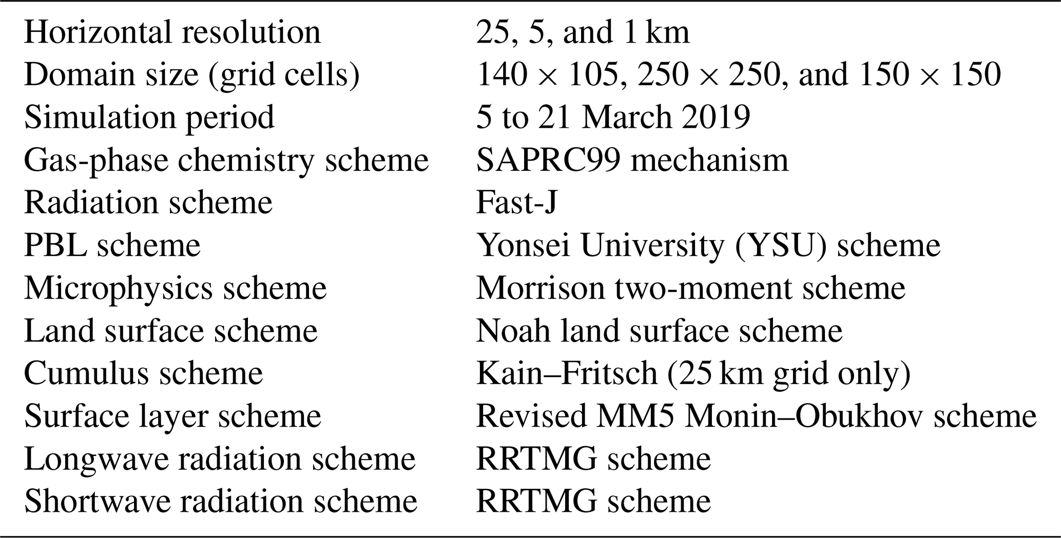
The configuration of WRF-Chem in this study is given in Table 1. The SAPRC99 photochemical mechanism (Carter, 2000) is chosen to simulate the gas-phase chemistry, and MOSAIC is selected for aerosol processes (Zaveri and Peters, 1999; Zaveri et al., 2008). The MOSAIC aerosol scheme includes important physical and chemical processes such as nucleation, condensation, coagulation, aqueous-phase chemistry, and water uptake by aerosols. Sulfate, nitrate, ammonium, sea salt, mineral dust, organic matter (OM), BC, and other (unspecified) inorganics (OIN) constitute the prognostic species in MOSAIC. The aerosol direct effect is coupled to the Rapid Radiative Transfer Model (RRTMG) (Mlawer et al., 1997; Iacono et al., 2000) for both SW (shortwave) and LW (longwave) radiation, as implemented by Zhao et al. (2011). We also turned on the aerosol indirect effect, which represents the interactions between aerosols and clouds, including the first and second indirect effects, activation/resuspension, wet scavenging, and aqueous chemistry (Gustafson et al., 2007; Chapman et al., 2009). The photolysis rate is computed by the Fast-J radiation parameterization (Wild et al., 2000). Our simulation includes the secondary organic aerosol (SOA) mechanism, a crucial aerosol process that can substantially reduce discrepancies between simulated results and observations.

Table 1 WRF-Chem model configuration.

Another type of option is meteorological physics, including the Yonsei University (YSU) nonlocal PBL parameterization scheme (Hong et al., 2006), the Noah land surface model (Chen and Dudhia, 2001) for the surface layer process, the Morrison two-moment scheme (Morrison et al., 2009) for cloud microphysics, and the Rapid Radiative Transfer Model (RRTMG) for LW and SW radiation. The 25 km resolution simulation turns on the option of cumulus parameterization, which uses the Kain–Fritsch cumulus and shallow convection scheme (Kain, 2004) to simulate sub-grid-scale clouds and precipitation. However, this option is turned off in the other two higher-resolution simulations because a fine resolution is sufficient to resolve the cloud-forming processes.

2.1.2 Numerical experiments

The study period spans from 5 to 20 March 2019. Following previous research (Gustafson et al., 2011), the first 5 d are considered to be the model spin-up time, while the remaining integration period is used for analysis. Consequently, only the results from 10 to 20 March 2019 are used in the analysis of this study. Three different resolutions and computational domains are employed in our study. The outer domain, covering East, North, and South China, has 140 × 105 grid cells (17.1–44.9° N, 107.1–127.9° E) with a horizontal resolution of 25 km. The middle domain, encompassing the entire YRD region in East China, has 250 × 250 grid cells (27.02–36.98° N, 111.82–121.78° E) with a resolution of 5 km. The inner domain, covering most of the Hefei region, consists of 150 × 150 grid cells (31.204–32.396° N, 116.604–117.796° E) at a horizontal resolution of 1 km. The center of the inner domain is the city of Hefei, a typical megacity of East China. Hefei, the capital city of Anhui Province, is located in the midlatitude zone with a humid subtropical monsoon climate and serves as a representative case for this study. The regions are shown in Fig. S1 in the Supplement. To facilitate the comparison of discrepancies among the three simulations at different resolutions, we have selected the innermost region as the main scope of study for this research, as shown in Fig. 1a.

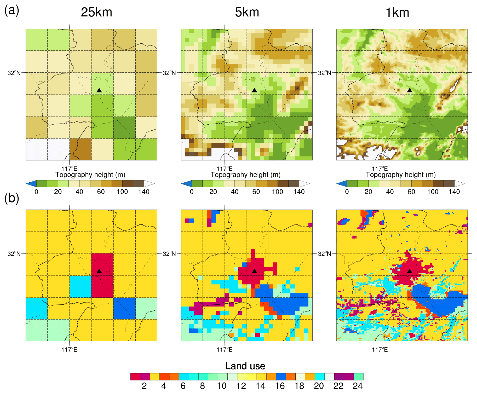
Figure 1 (a) The terrain height (m) in the study area for simulations with respective resolutions of 25 km (left), 5 km (middle), and 1 km (right). (b) Spatial distribution of land use types in the study area for simulations with respective resolutions of 25 km (left), 5 km (middle), and 1 km (right). The solid black triangle indicates the location of the USTC site.

In this study, we derive terrain information from high-resolution (∼ 1 km) US Geological Survey (USGS) topographic data and interpolate it onto the WRF grid. Therefore, the three domains with different resolutions exhibit varying degrees of terrain detail. The 1 km grid resolves the most intricate topographic features, followed by the 5 km grid, while the 25 km grid captures the least spatial detail. These multiple-resolution topographic representations potentially influence pollutant turbulent mixing processes, which will be analyzed in this study. The land cover dataset is derived from a 1 km horizontal resolution dataset for China (Zhang et al., 2021). The land use categories follow the USGS 24-category classification, and the dataset is based on China's land cover conditions as of 2015. This provides a more accurate representation of current land cover, particularly for eastern China, which has experienced intensive urban expansion since the 2000s. Figure 1b shows the land cover data at different resolutions, with detailed descriptions of the legend and land cover classes provided in Table S1 in the Supplement. This set of simulations is referred to as the “baseline experiment”. With the exception of part of Sect. 3.2.3, all other analyses in this study are based on the results of these baseline experiments. Moreover, to explore the differences in turbulent mixing simulated at multiple resolutions under consistent land use conditions, we conducted an additional set of sensitivity experiments referred to as the “sensitivity experiment”. The sensitivity experiment was identical to the baseline experiment, except it used the default USGS land use category data in WRF. Notably, these default USGS data in WRF's geographical static database represent Chinese land use patterns before the 2000s, as shown in Fig. S2. This default dataset reflects the land use distribution prior to China's significant urbanization. Consequently, the land use data types have minor variations and remained generally consistent across all three resolutions in the sensitivity experiment.

On the other hand, the vertical configuration within the PBL is also crucial for accurately modeling pollutant dispersion. To better resolve the PBL structure and mixing processes, we implemented a finer vertical resolution within the PBL. Identical vertical layer distributions are maintained across all three horizontal resolutions (25, 5, and 1 km), ensuring direct comparability of turbulent mixing across different horizontal resolutions. A total of 50 terrain-following vertical η layers extending from the surface to approximately 15 km were used in all three resolution simulations, with 30 layers distributed below 2 km above the ground to describe the atmospheric boundary structure in detail. The vertical layer was strategically designed with seven layers below 200 m (each approximately 20 m in height), three layers between 200 and 300 m (each about 30 m in height), and eight layers between 300 and 1000 m (each approximately 80 m in height). This configuration comprehensively captures mixed-layer development and key turbulent processes (e.g., entrainment and surface flux exchange) through layer densification, which is sufficient to capture PBL turbulent mixing. Jiang et al. (2024) and Jiang and Hu (2023) have demonstrated that the number of model vertical layers primarily influences the vertical distribution, with more vertical grid layers producing a more stable vertical structure under stable boundary conditions that better resolves boundary layer turbulence.

In order to allow for a straightforward comparison of multiple-resolution simulations and facilitate the identification of differences between the high- and low-resolution simulations, the corner locations of the 1 and 5 km resolution domains are aligned with the corner locations of the 25 km grid cell. Each grid cell in the 25 km simulation consists of a 5 × 5 set of cells from the 5 km simulation, and each grid cell in the 5 km simulation comprises 5 × 5 cells from the 1 km simulation, as shown in Fig. S3. Thus, exactly 25 grids at 5 km resolution and 625 grids at 1 km resolution are embedded within each 25 km grid cell.

To ensure similar boundary forcing across the three simulations, initial and boundary conditions are handled differently for the 25, 5, and 1 km resolution domains. For the 25 km resolution, meteorological initial and lateral boundary conditions are obtained from the National Center for Environmental Prediction (NCEP) Final (FNL) reanalysis data with a 1° × 1° resolution and 6 h temporal resolution. Initial and boundary conditions for the trace gases and aerosol species are provided by the quasi-global WRF-Chem simulation with 360 × 145 grid cells (67.5° S–77.5° N, 180° W–180° E) at a 1° × 1° resolution. The initial and boundary conditions for the simulation at 5 km resolution are derived from the simulation at 25 km resolution. Similarly, the initial and boundary conditions for the simulation at 1 km resolution are derived from the simulation at 5 km resolution. In this way, as the forcing for the study area is consistent across multiple resolutions, differences in simulation results among multiple resolutions can be attributed to disparities in model resolutions.

2.1.3 Emissions

Anthropogenic emissions for the outer quasi-global simulation are derived from the Hemispheric Transport of Air Pollution version-2 (HTAPv2) emission inventory at a 0.1° × 0.1° horizontal resolution and monthly temporal resolution for 2010 (Janssens-Maenhout et al., 2015). The Multi-resolution Emission Inventory for China (MEIC) at a 0.25° × 0.25° horizontal resolution for 2019 (Li et al., 2017a, b) is used to replace emissions over China within the simulation domain. Emission differences significantly contribute to pollutant concentration variability across multiple resolutions. Qian et al. (2010) showed that sub-grid variability in emissions can contribute up to 50 % of the variability near Mexico City. To eliminate the impact of inconsistent emissions on pollutant concentrations simulated at multiple resolutions, we ensured emission consistency across all three domains by interpolating emissions for all species from the 25 km resolution domain to both the 5 and 1 km resolution domains. This study primarily focuses on BC. The spatial distribution of BC emissions is shown in Fig. 2. Figure S4 illustrates BC emissions at three different resolutions, demonstrating similar spatial patterns across multiple resolutions. Biomass-burning emissions are obtained from the Fire Inventory from NCAR (FINN) at a 1 km horizontal resolution and 1 h temporal resolution (Wiedinmyer et al., 2011). The diurnal variation in biomass-burning emissions follows the suggestions by WRAP (2005), with injection heights based on Dentener et al. (2006) from the Aerosol Comparison between Observations and Models (AeroCom) project. Biogenic emissions were calculated using the Model of Emissions of Gases and Aerosols from Nature (MEGAN) version 3.0 (Guenther, 2006; Zhang et al., 2021).

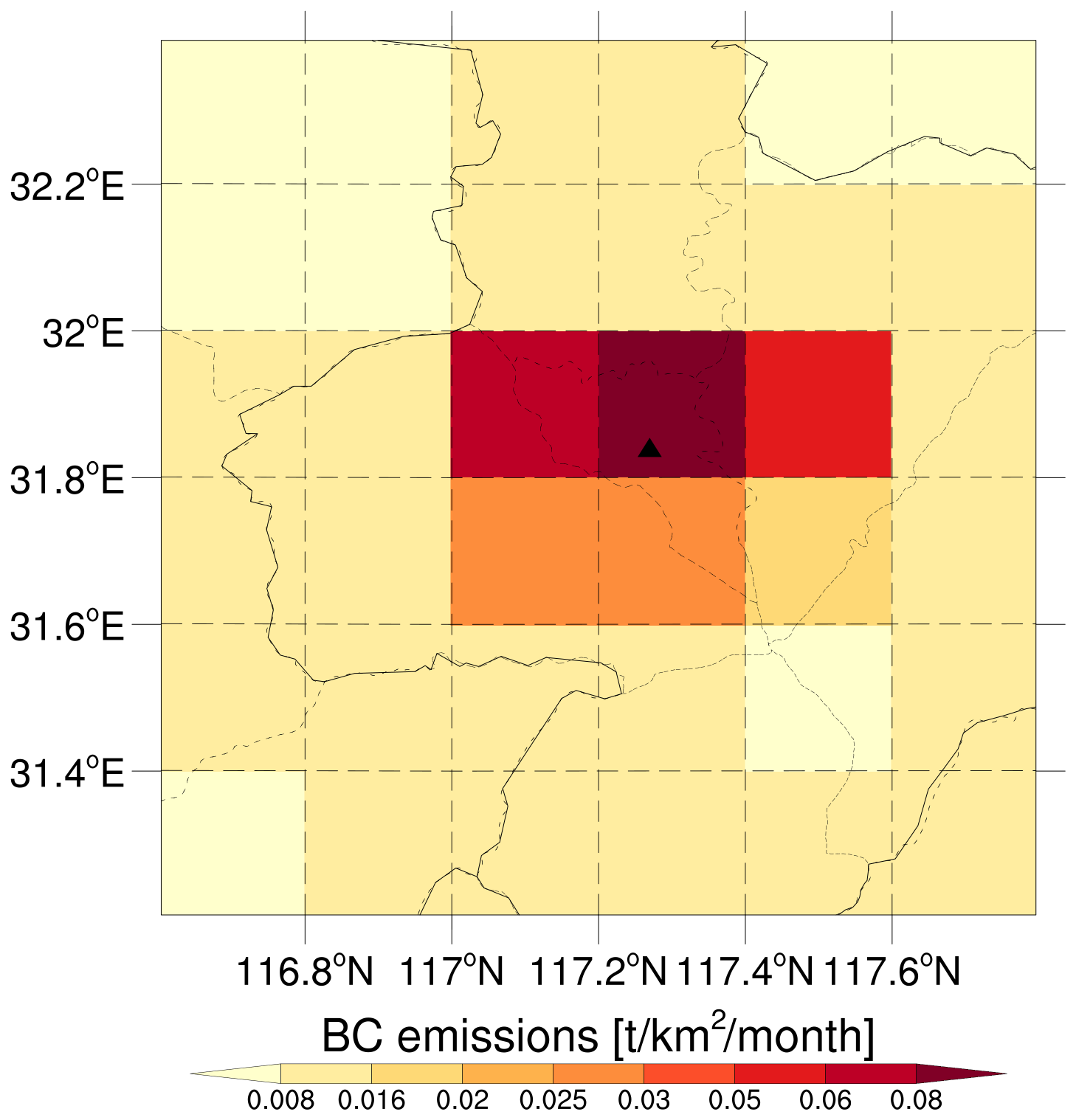
Figure 2 Spatial distribution of BC emissions in the study area. The solid black triangle indicates the location of the USTC site.

2.2 Observational data

2.2.1 Meteorological data

The meteorological data were obtained from the observation tower at the University of Science and Technology of China (USTC) in Hefei, Anhui, China (31.84° N, 117.27° E), indicated by a solid black triangle in Fig. 1a. The tower measures temperature, relative humidity, wind speed, and wind direction at 2, 4.5, 8, 12.5, and 18 m heights. This site represents a typical urban surface within the study area. The tower was installed on the roof of a teaching building, with its top 17 m above the canopy plane. It is equipped with three R.M. Young 03002 anemometers and three HPM155A temperature and humidity sensors to measure the aforementioned meteorological parameters (Yuan et al., 2016; Liu et al., 2017). This study focuses on analyzing temperature, relative humidity, and wind speed.

Additionally, we employed meteorological data from automatic weather stations (AWSs), which were established based on the operational standards issued by the China Meteorological Administration (CMA, 2018). The hourly data underwent quality control (QC) by the local meteorological bureaus of Anhui, following World Meteorological Organization guidelines (Estevez et al., 2011). The QC included checks of consistency, such as internal, temporal–spatial, and climatic range validations. These QC data were used to determine daily mean, minimum, and maximum meteorological variables. The AWSs recorded various parameters, including air temperature (T, °C), wind speed (U, m s⁻¹), air pressure (P, Pa), and wind direction. In this study, we focus on the 3-hourly 2 m temperature and 10 m wind speed obtained from four AWSs located in the study region. The four AWS sites are marked by solid purple dots in Fig. S5.

2.2.2 Pollutant data

We used the hourly BC observations from the air quality monitoring site on the campus of USTC during spring (10 to 20 March 2019). In this study, we focus on analyzing BC observational data and comparing them with model output. BC was observed using a multi-angle absorption photometer (MAAP, Model 5012) manufactured by Thermo Scientific. This instrument is located approximately 260 m north of the USTC meteorological tower. It takes advantage of the strong visible light absorption properties of BC aerosols. There is a linear relationship between the attenuation of the beam after passing through the aerosol sample and the load of BC aerosols on the fiber membrane. The BC concentration is derived by inverting this relationship. A light-scattering measurement is incorporated into the chamber to correct for multiple-scattering effects caused by particle accumulation on the filter tape. The MAAP-5012 black carbon meter collects atmospheric aerosols using glass fiber filter membranes and observes them at a wavelength of 670 nm.

Although this study primarily focuses on the simulation of BC, we conducted a comprehensive validation of other air pollutants to ensure the reliability of the simulation results. However, after being initially obtained via a parameterized PBL scheme, the mixing coefficients for gases are then clipped to empirically chosen thresholds of 1 m² s⁻¹ over rural regions and 2 m² s⁻¹ over urban regions, with the distinction between rural and urban regions made based on the local CO emission strength. Thus, the boundary layer mixing coefficient for gases in the WRF-Chem model is implicitly influenced by emission resolution rather than directly controlled by model resolution. Consequently, the existing adjustment process for gas mixing coefficients, which relies on CO emission strength, is unsuitable for studying the impact of model resolution on the turbulent mixing of gaseous pollutants. In contrast, the mixing coefficients for particulate matter are directly calculated through boundary layer parameterization without subsequent modifications. The publicly available version of WRF-Chem defines a default lower limit of 0.1 m² s⁻¹ for particulate matter mixing coefficients. We did not implement the adjustment proposed by Du et al. (2020), who suggested raising the lower limit of the PBL mixing coefficient from 0.1 to 5 m² s⁻¹ within the PBL. Although setting specific thresholds can improve simulation results, such thresholds are predominantly empirical in nature, whether based on CO and PM_2.5 emissions or the 5 m² s⁻¹ threshold suggested by Du et al. (2020). These threshold adjustments effectively compensate for missing physical processes in the model by artificially enhancing mixing intensity. Our approach focuses on understanding the physical mechanisms responsible for the model's underestimation of nighttime mixing intensity, with a particular emphasis on how the model resolution affects turbulent mixing processes. Rather than employing empirical thresholds to align model output with observations, we aim to investigate the fundamental causes of the discrepancies. We contend that threshold approaches rely heavily on empirical data, lack sufficient theoretical foundation, and may impede comprehensive understanding of the underlying physical processes. Consequently, this work utilizes the default particulate matter turbulent mixing coefficients in the model for our analyses. In this study, we limited our additional validation to PM_2.5 (fine particulate matter with an aerodynamic diameter of less than 2.5 µm), as its mixing processes are governed by the same resolution-dependent mechanisms as BC. Ground observations of hourly PM_2.5 surface concentrations during March 2019 were obtained from the website of the Ministry of Environmental Protection of China (MEP of China). As our study concentrates on the Hefei region, we selected 10 monitoring stations within this area for detailed analysis. These stations are marked using black triangles in Fig. S5.

While hourly observations for both meteorology and pollutants are available, model outputs are provided at 3 h intervals to balance computational efficiency and storage requirements. Hourly output data would provide a higher temporal resolution but would significantly increase storage demands. Given that we ran simulations at multiple resolutions (25, 5, and 1 km), hourly outputs would have generated prohibitively large data volumes. On the other hand, this 3 h output interval remains sufficient for our primary research objective of analyzing daily pollutant variations (particularly BC) rather than precise hourly comparisons. This approach effectively captures daily variability patterns without losing essential detail. For direct comparisons, hourly observations were sampled to match our 3 h model output intervals.

3 Results

3.1 Simulated meteorological fields at various horizontal resolutions

Meteorological fields may play a crucial role in turbulent mixing and pollutant transport. In this study, we evaluate time series of simulated temperature, wind speed, and relative humidity across three resolutions against observational data to assess resolution impacts on these key meteorological variables. Figure 3a compares the time series of observed and simulated 8 m wind speeds at the USTC site (31.84° N, 117.27° E). Simulation results among multiple resolutions are similar, which is attributed to the relatively flat and uncomplicated topography. The temporal trends in the simulations closely align with observational data, exhibiting distinct diurnal variations characterized by higher values during the daytime and lower values at night. Additionally, the model struggles to capture some moments accurately, overestimating wind speed when it suddenly increases. For instance, at noon on 20 March, while the observed peak wind speed was approximately 6 m s⁻¹, simulations at 25 and 5 km resolutions produced maximum wind speeds of approximately 9 m s⁻¹, significantly exceeding the observed value, with only the 1 km resolution simulation yielding results close to the observation. Figure 3b compares the 2 m temperature simulated at three different resolutions with the observations. The multiple-resolution simulation results exhibit remarkable consistency and closely align with observations. Temperature displays a pronounced diurnal variation, fluctuating between 5 and 30°C with relative stability. However, the model occasionally underestimates or overestimates values at certain time points. As shown in Fig. 3c, the multiple-resolution simulation results demonstrate consistency and accurately capture the diurnal variation trend in the observed relative humidity (RH). Model results are highly consistent with observations, with both reaching a maximum of 100 %.

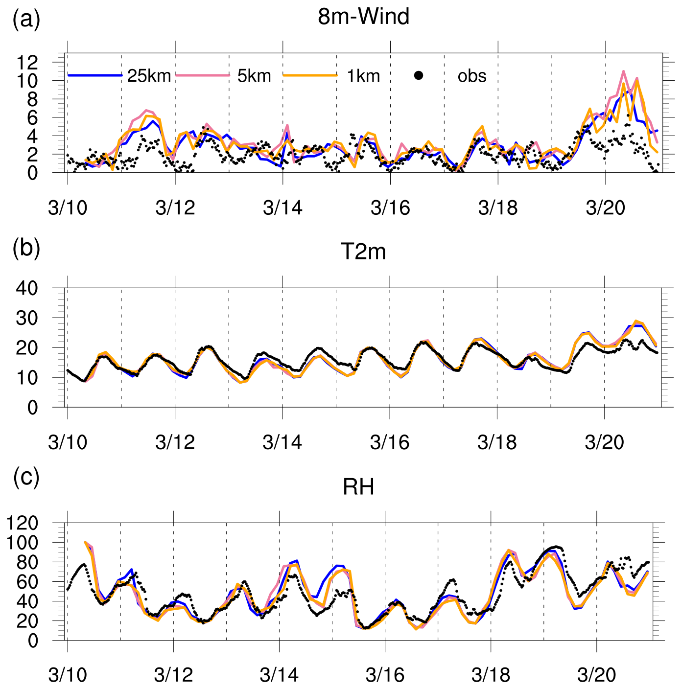
Figure 3 USTC meteorological tower observation site time series of observed (black dot) and simulated wind speed at (a) 8 m (unit: m s⁻¹), (b) temperature at 2 m (unit: °C), and (c) relative humidity (unit: %) at respective resolutions of 25 km (solid blue line), 5 km (solid pink line), and 1 km (solid orange line).

Additionally, Fig. S6 displays the time series of observed and simulated meteorological variables averaged across four AWSs in the study region. Figure S6a presents a comparison of the 10 m wind speed simulated at three different resolutions, revealing generally consistent results with observations. The overall pattern is similar to that observed at the single USTC station, characterized by a clear diurnal variation with higher wind speeds during daytime and lower speeds at night. However, simulations at all three resolutions occasionally deviate from observations. For example, on 11 March, the 5 and 1 km resolution models overestimate the wind speed at approximately 7 m s⁻¹ compared to the observed 4 m s⁻¹. Conversely, on 14 March during the daytime, all three resolutions underestimate the wind speed, simulating around 2 m s⁻¹ against an observed value of 4 m s⁻¹. Figure S6b compares the simulated 2 m temperatures across three resolutions with observational data. The simulated temperatures are remarkably similar across all resolutions and show a strong correlation with observations throughout most of the study period. Only a few outliers were noted, which minimally impact the overall pattern. For example, models at all resolutions overestimate the temperature at noon on 20 March, simulating approximately 28 °C, whereas the observed temperature is only about 20 °C.

In summary, the simulated meteorological variables across multiple resolutions demonstrate strong similarity and closely match the observations, with only occasional minor discrepancies. However, our subsequent analysis reveals that the variations in pollutant concentrations across multiple resolutions cannot be attributed to the minor discrepancies observed in the time series of meteorological variables.

3.2 Simulated BC surface concentrations and impacts of turbulent mixing at various horizontal resolutions

3.2.1 Surface concentrations simulated at three different horizontal resolutions

The spatial distribution of BC surface concentrations across multiple resolutions in the study area is illustrated in Fig. 4. As the resolution improves from 25 to 5 km and further to 1 km, BC surface concentrations reveal more detailed spatial features. Figure 4a presents the simulation results across multiple resolutions, averaged over the whole day. Significant variations exist from coarse resolutions to fine resolutions, with surface concentrations decreasing as resolution increases from 25 to 5 km and further to 1 km. BC surface concentrations range from 0 to 9 µg m⁻³. At 25 km resolution, there is a notable discrepancy between the spatial distributions of BC concentrations and emissions (Fig. 2). The highest simulated concentration at 25 km resolution is located west of the USTC site, while maximum emissions are centered at the USTC site. Our analysis indicates that the difference in turbulent mixing between these two regions leads to spatial inconsistency between BC surface concentrations and emissions. The details of this phenomenon will be discussed in Sect. 3.2.2. Figure 4b illustrates the spatial distribution of BC surface concentrations during the daytime. The differences in surface concentrations among multiple resolutions are minimal, with values falling within the range of 0 to 5 µg m⁻³. In the central urban areas, the BC surface concentration simulated at a 25 km resolution is marginally lower than those simulated at finer resolutions. Moreover, during the daytime, simulated BC concentrations over the Chaohu Lake area are notably higher than in other regions, potentially due to the impact of dry deposition velocity. Figure S7 shows the spatial distribution of dry deposition velocity, revealing lower values over lakes compared to other areas. This lower dry deposition velocity leads to higher pollutant concentrations over lakes compared to land areas after pollutant transport to the lake surface during the daytime. At night, dry deposition velocity is similar to that of surrounding nonurban land areas. Consequently, nighttime BC concentrations over lakes are approximately equal to those in surrounding areas. Figure 4c demonstrates the spatial distribution of BC surface concentrations during nighttime. Compared to daytime, BC surface concentrations are notably higher in all major urban regions at night, with high-resolution simulations capturing more spatial variation. In conclusion, BC surface concentrations decrease as the resolution increases from 25 to 5 km and further 1 km. However, the spatial distribution of BC surface concentrations at resolutions of 5 and 1 km are similar throughout the whole day.

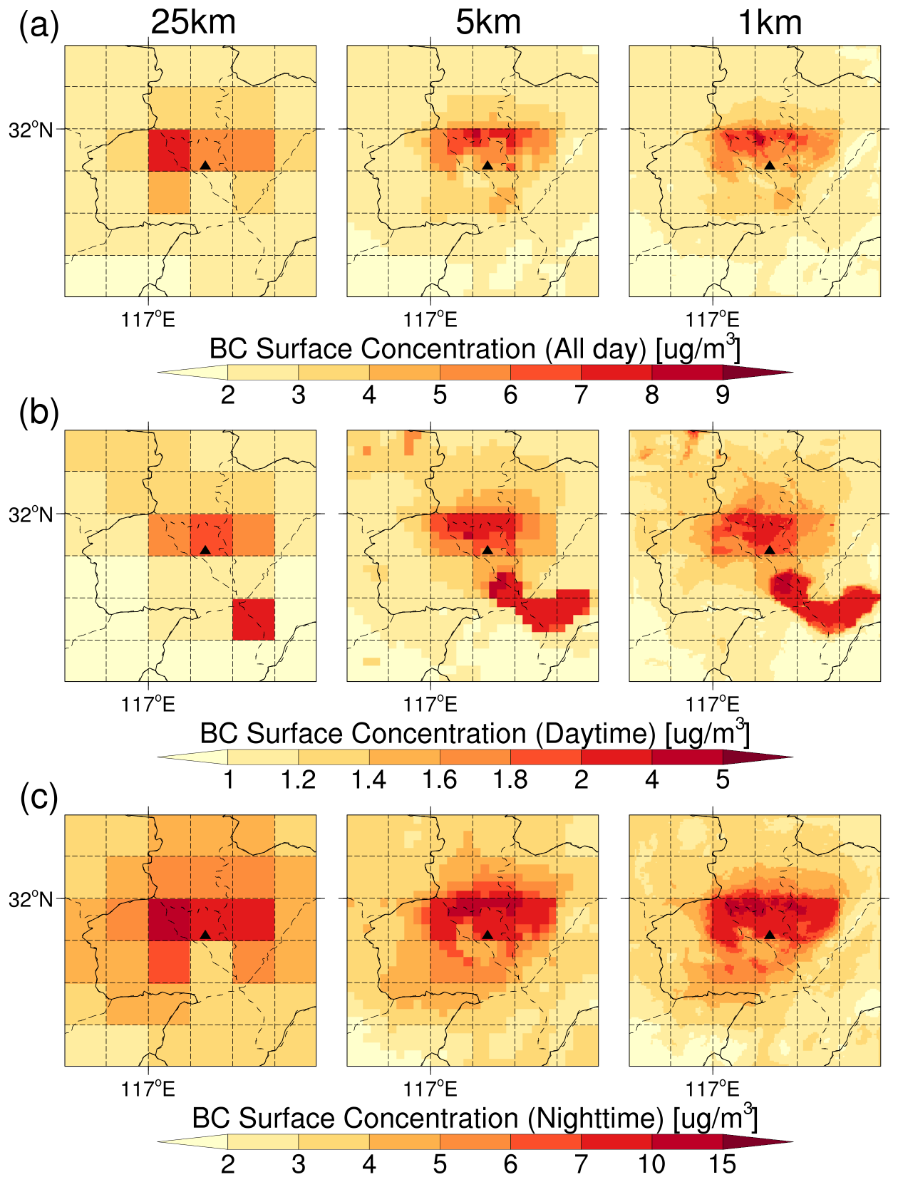
Figure 4 Spatial distribution of the BC surface concentration in the study area for 25 km (left), 5 km (middle), and 1 km (right) resolution simulations of (a) the whole day, (b) daytime, and (c) nighttime, respectively. The solid black triangle indicates the location of the USTC site.

To facilitate a more accurate and direct comparison of results across multiple resolutions, we refine coarse grids to match fine grids. The detailed refinement process is described in Sect. S1 in the Supplement. Figure S8a exhibits the spatial differences in BC surface concentrations between resolutions of 25 and 5 km and between resolutions of 25 and 1 km averaged over the whole day. It reveals that coarse-resolution (25 km resolution) simulations generally yield higher BC surface concentrations than fine-resolution (5 and 1 km resolution) simulations across most areas. The largest disparities mainly occur in central urban areas with complex underlying surfaces and complicated flow patterns. Figure S8b demonstrates the spatial differences in BC surface concentrations between resolutions of 25 and 5 km and between resolutions of 25 and 1 km during the daytime, revealing smaller disparities mostly ranging between −1 and 1 µg m⁻³. In contrast, Fig. S8c depicts pronounced differences in BC concentrations between resolutions of 25 and 5 km and between resolutions of 25 and 1 km during the nighttime, with most areas exhibiting disparities exceeding 2 µg m⁻³. The largest differences are mainly concentrated in urban areas. These findings indicate that diversities in BC surface concentrations among multiple resolutions are primarily attributable to nocturnal concentrations in urban areas. However, differences between 5 and 1 km resolutions are small compared to those between 25 km and finer resolutions (5 and 1 km). BC surface concentrations are approximately equal in the 5 and 1 km simulations, as shown in Fig. S9.

Furthermore, BC observations from the USTC monitoring station were utilized to validate the simulated BC surface concentrations. Figure 5 illustrates the diurnal variation in BC surface concentrations averaged over the USTC site. Both observations and simulations exhibit a pronounced diurnal variation, with lower concentrations during the daytime and higher concentrations at night. During the daytime, BC surface concentrations simulated at three resolutions are comparable to the observational data. However, nighttime simulations significantly overestimate BC surface concentrations. As resolution increases from 25 to 5 and 1 km, the simulated surface concentrations decrease, aligning more closely with observations. The 25 km resolution simulations yield the highest concentrations, with a maximum value of approximately 12 µg m⁻³, nearly double the observed values. In contrast, BC surface concentrations simulated at 5 and 1 km resolutions are similar and more closely align with nocturnal observations, peaking at around 9 µg m⁻³. In conclusion, the diurnal variation in the observation is better captured by high-resolution (5 and 1 km) simulations. The performance of BC surface concentrations across multiple resolutions demonstrates that a coarse grid spacing inadequately captures local pollutant distributions.

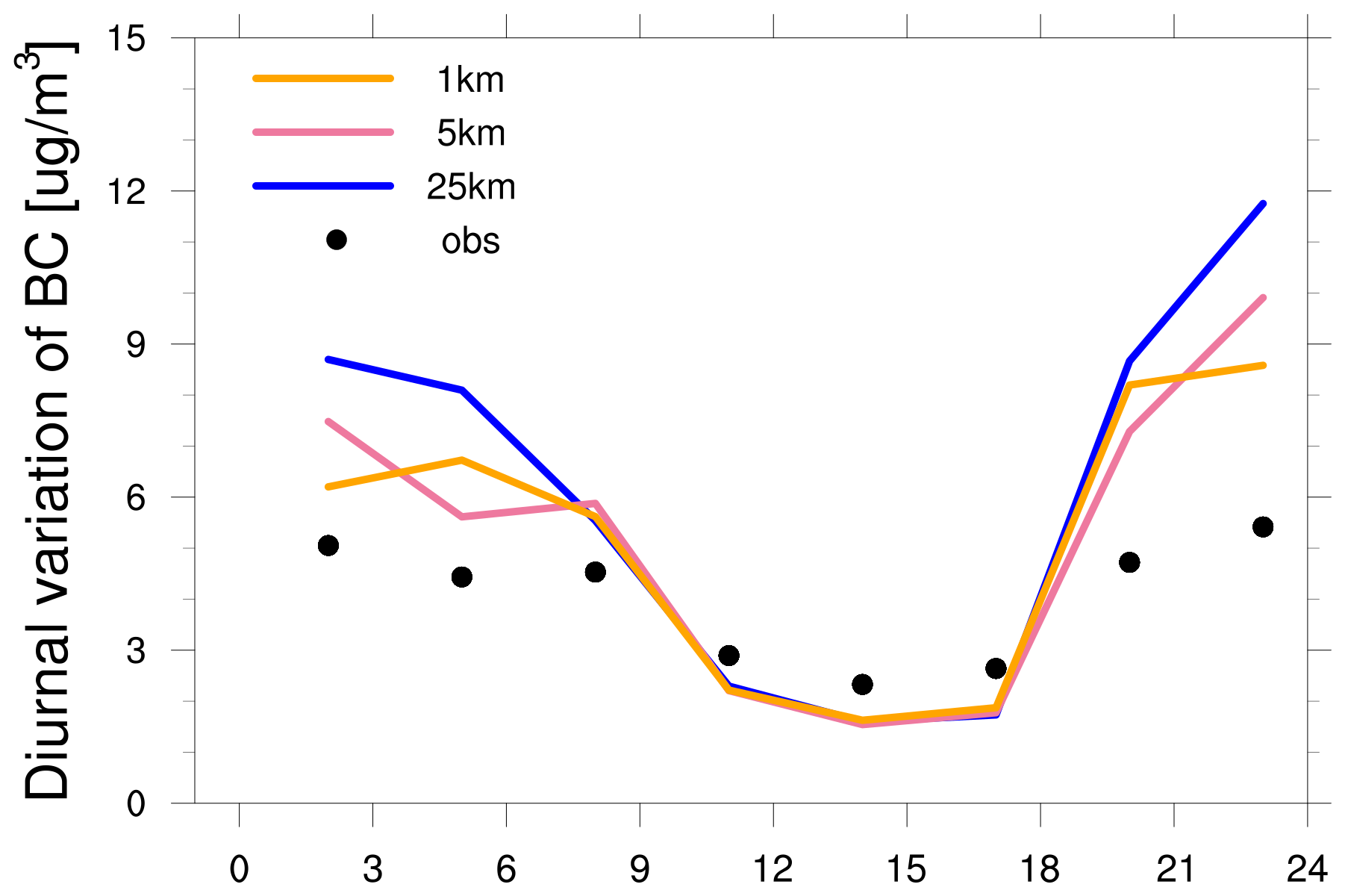
Figure 5 Diurnal variation in BC surface concentrations within 24 h averaged over the USTC site during the study period for 25 km (solid blue line), 5 km (solid pink line), and 1 km (solid orange line) resolution simulations and observations (black dot). Both the simulated results and observations are sampled at the model output frequency, i.e., 3 h.

To verify the accuracy and comprehensiveness of the simulation results, we further analyzed the diurnal variation in PM_2.5 surface concentrations. Figure S10 illustrates the diurnal variation in simulated PM_2.5 surface concentrations across multiple resolutions compared with observations. The diurnal pattern of PM_2.5 closely resembles that of BC, characterized by higher concentrations at night and lower concentrations during daytime. Across all resolutions, the model slightly underestimates daytime PM_2.5 surface observations while overestimating nighttime values. Notably, an increased horizontal resolution substantially improves nocturnal simulations. The 25 km resolution simulation generates an anomalous midnight peak (105 µg m⁻³), resulting in a +61 % bias, whereas the 5 and 1 km resolutions substantially mitigate these deviations to approximately 30 %. To further examine the contribution of each PM_2.5 component to the diurnal variation across multiple resolutions, Fig. S11 shows the diurnal variations in four PM_2.5 constituents – sulfate (${\mathrm{SO}}_{\mathrm{4}}^{\mathrm{2}-}$), nitrate (${\mathrm{NO}}_{\mathrm{3}}^{-}$), OIN, and organic carbon (OC) – averaged over 10 MEP sites in Hefei. Significant differences emerge in the diurnal variations in these components across multiple-resolution simulations. Specifically, the surface concentrations of ${\mathrm{NO}}_{\mathrm{3}}^{-}$, OIN, and OC exhibit a consistent diurnal pattern, with lower concentrations during daytime and higher concentrations at night. As resolution increases from 25 to 5 and 1 km, the simulated components surface concentrations decrease, aligning more closely with observations.

The total concentration of PM_2.5 and its components demonstrates significant sensitivity to horizontal resolutions. Coarse-resolution simulations underestimate the turbulent mixing capacity, resulting in overestimated concentrations. Higher-resolution simulations more accurately capture vertical mixing within the PBL. For secondary particles such as sulfates and nitrates, formation rates depend heavily on local precursor substance concentrations (SO₂ and NO_x). Higher-resolution simulations may enable the more realistic representation of precursor substance diffusion, leading to reduced local concentration gradients and, consequently, slower secondary aerosol formation rates. Additionally, variations in PM_2.5 surface concentrations across multiple resolutions may also stem from complex secondary particle generation mechanisms. For instance, the liquid-phase oxidation of sulfates in clouds is sensitive to the local cloud water distribution, with higher resolutions better capturing small-scale cloud structures that potentially alter the sulfate formation efficiency. The formation of ammonium nitrate (NH₄NO₃) is particularly sensitive to temperature and humidity variations. At higher resolutions, temperature and humidity gradients induced by urban heat island effects or topographical variations can be more realistically simulated, influencing the distribution of gaseous nitric acid (HNO₃) and particulate nitrate (${\mathrm{NO}}_{\mathrm{3}}^{-}$). Dry deposition processes may also contribute to resolution-dependent variations, as local differences in surface roughness (including buildings and vegetation) become more apparent at higher resolutions, directly affecting particulate deposition velocity rates. Overall, the simulation results for major air pollutants fall within a reasonable error range compared to observational data, confirming the reliability of the model for this study.

We now aim to further investigate the underlying factors contributing to the discrepancies in atmospheric pollutant simulations, with a particular focus on BC, across different spatial resolutions. Previous studies have indicated that the diurnal variation in atmospheric particulate matter concentrations is primarily controlled by daily variations in PBL mixing and pollutant emissions (Du et al., 2020). The diurnal variation in BC emissions peak during the daytime and are lower at night. During nighttime, pollutants are trapped within the shallow boundary layer due to reduced turbulent mixing, resulting in elevated surface concentrations of atmospheric particulate matter. As the boundary layer develops in the morning, pollutants rapidly diffuse and are transported to upper atmospheric layers, leading to relatively low surface concentrations. Therefore, the turbulent mixing process plays a crucial role in determining pollutant concentrations.

3.2.2 Impacts of turbulent mixing on BC surface concentrations at three different horizontal resolutions

To investigate the vertical mixing depth influencing pollutant diffusion, we first analyze the PBL height, as illustrated in Fig. 6. Figure 6a shows the spatial distribution of the PBL height simulated at three different resolutions, averaged over the whole day. Higher-resolution simulations yield lower PBL heights and capture more intricate details compared to lower-resolution simulations. This trend is consistent during both daytime and nighttime. Figure 6b demonstrates that the PBL height exceeds 0.9 km across most regions during the daytime. Notably, due to strong topographic influences, the PBL height in the vicinity of Chaohu Lake is remarkably low, typically less than 0.1 km. Conversely, in the southwestern region, characterized by higher elevations and more complex terrain, the PBL height surpasses 1.1 km. Figure 6c depicts the nighttime PBL heights at three different resolutions. These heights predominantly fall below 0.3 km, significantly lower than those during the daytime. The PBL height gradually decreases as the resolution increases, which should typically lead to higher BC surface concentrations. However, BC surface concentrations actually decrease as resolution increases from 25 to 5 and 1 km (Fig. 4). Consequently, the PBL height alone cannot explain the differences in pollutant simulations among the multiple resolutions in this study.

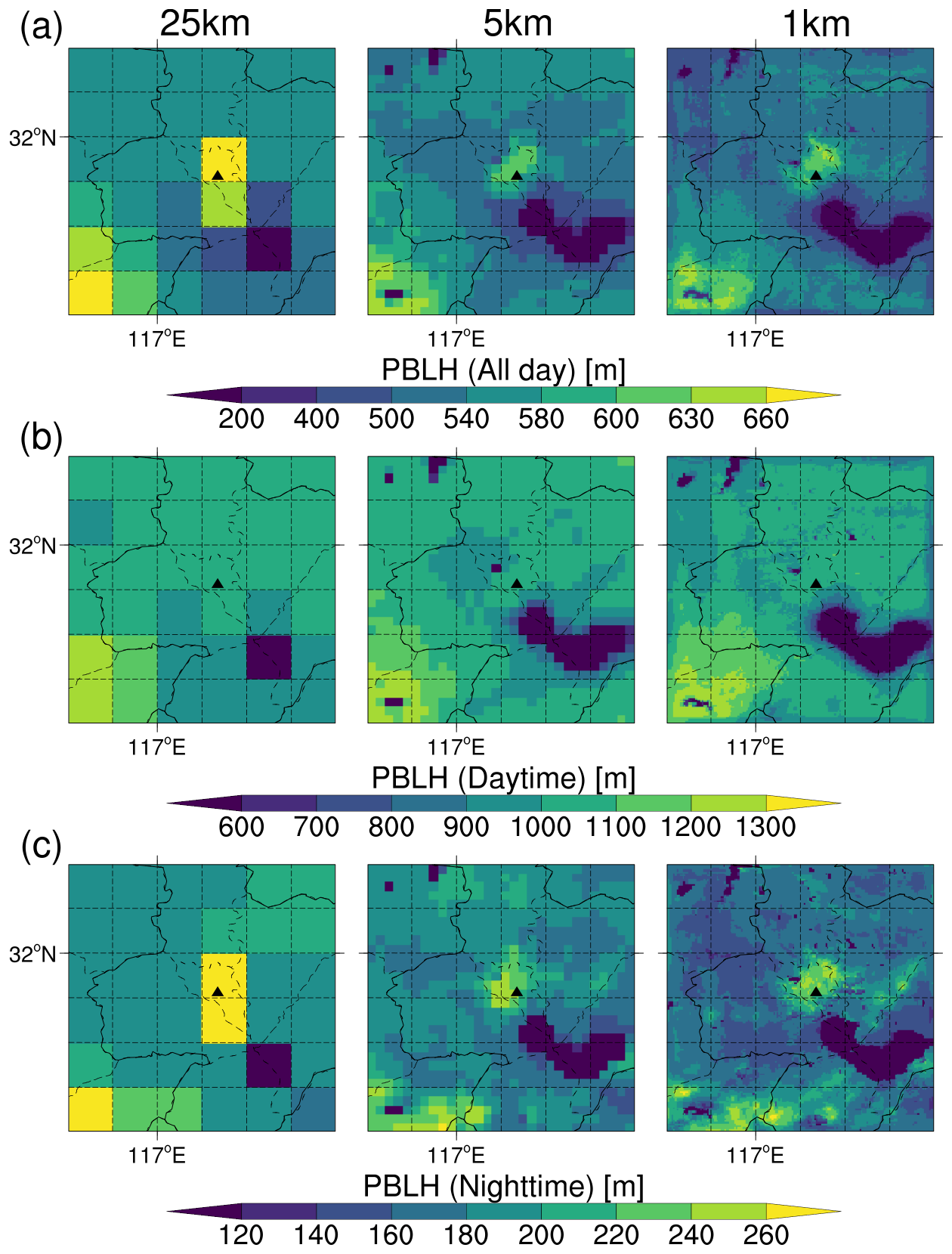
Figure 6 Spatial distribution of the PBL height in the study area for 25 km (left), 5 km (middle), and 1 km (right) resolution simulations of (a) the whole day, (b) daytime, and (c) nighttime, respectively. The solid black triangle indicates the location of the USTC site.

Previous studies have established that PBL mixing coefficients are critical determinants in air quality modeling (Du et al., 2020). In WRF-Chem, turbulent mixing within the boundary layer is partially governed by PBL mixing coefficients generated by the PBL parameterization scheme. It is worth noting that the mixing coefficients for atmospheric particulate matter and gases are two distinct variables in the current version of WRF-Chem. The boundary layer mixing coefficient for gases is initially obtained via a parameterized PBL scheme but undergoes additional modification through an empirical parameterization that enhances gas mixing based on CO emission strength (Kuhn et al., 2024). This enhancement applies to gas pollutants when using the MOSAIC aerosol scheme, as implemented in this study. Specifically, gas mixing coefficients are clipped to empirically chosen thresholds of 1 m² s⁻¹ over rural regions and 2 m² s⁻¹ over urban regions, with the distinction between rural and urban regions made based on the local CO emission strength. In contrast, the mixing coefficient of particulate matter is directly calculated through boundary layer parameterization without subsequent modifications. Our study focuses exclusively on the turbulent mixing of atmospheric particulate matter, analyzing the aerosol mixing coefficient with the default lower limit of 0.1 m² s⁻¹ as specified in the publicly released version of WRF-Chem. We have not implemented the mixing coefficient adjustments proposed by Du et al. (2020), who suggest raising the lower limit of PBL mixing coefficient from 0.1 to 5 m² s⁻¹ within the PBL. We contend that threshold approaches are primarily based on empirical data and may impede a comprehensive understanding of the underlying physical processes. In our study, particulate matter mixing coefficients are directly calculated through boundary layer parameterization without adjustments based on empirical settings. This approach allows the model to more accurately represent the natural turbulent mixing processes. Consequently, we can investigate the turbulent mixing intensity of particulate matter across different horizontal resolutions and examine the true impact of grid resolution on pollutant mixing.

The spatial distribution of aerosol turbulent mixing coefficients at the lowest model layer is analyzed, as shown in Fig. 7. Figure 7a illustrates the simulation results across multiple resolutions averaged over the whole day. The variations in the PBL mixing coefficients across different resolutions are evident, with high-resolution simulations capturing more spatial characteristics. The spatial distribution of the PBL mixing coefficient demonstrates a strong correlation with land use type and terrain height, which will subsequently be explored. Turbulent mixing coefficients range from 0 to 8 m² s⁻¹, with peak values predominantly located in urban areas. Notably, the mixing coefficient simulated at a 25 km resolution near the surface around USTC substantially exceeds that of the western area, resulting in lower BC surface concentrations simulated at a 25 km resolution at USTC compared to its western regions (Fig. 4). This discrepancy leads to a mismatch between the spatial distribution of pollutant concentrations and emissions, as discussed in Sect. 3.2.1. During the daytime, the PBL mixing coefficients simulated at three resolutions are relatively high, ranging from 0 to 17 m² s⁻¹, as shown in Fig. 7b. BC masses simulated across multiple resolutions are fully mixed within the boundary layer, resulting in similar BC surface concentrations across these resolutions. Conversely, turbulent mixing coefficients diminish considerably during the nighttime, with maximum values of approximately 3 m² s⁻¹, as shown in Fig. 7c. The turbulent mixing coefficient emerges as one of the important factors controlling surface pollutant concentrations under stable nocturnal PBL conditions. Nighttime PBL coefficients are higher at resolutions of 5 and 1 km compared to a 25 km resolution across most of the study area, resulting in lower BC surface concentrations at these two higher resolutions during the nighttime. Figure S12 further illustrates the disparities in parameterized PBL mixing coefficients between a 25 km resolution and the two higher-resolution simulations. However, Fig. S13 shows that the turbulent mixing coefficient parameterized at a 5 km resolution is larger than that at a 1 km resolution, which fails to explain the similar surface concentrations in these two higher-resolution (5 and 1 km) simulations. To further investigate this phenomenon, we selected a meridional section passing through the USTC site to analyze the distribution of vertical wind speed flux, which represents the turbulent mixing directly resolved by large-scale dynamic processes.

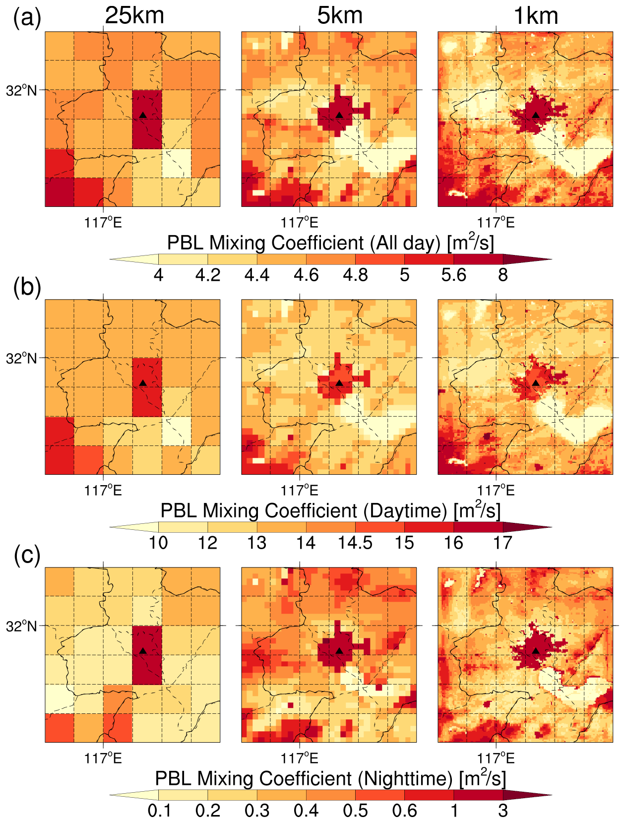
Figure 7 Spatial distribution of PBL mixing coefficients in the study area for 25 km (left), 5 km (middle), and 1 km (right) resolution simulations of (a) the whole day, (b) daytime, and (c) nighttime, respectively. The solid black triangle indicates the location of the USTC site.

Figure 8 displays the cross section of meridional wind speed flux along the USTC site simulated at three different resolutions. The upward vertical wind speed flux simulated at a 25 km resolution is near the surface. However, the 5 km resolution simulation generates stronger upward motion at a slightly higher altitude, specifically between 850 and 1000 hPa. Notably, the 1 km resolution simulation captures the highest vertical wind speed flux, with relatively intensive upward motion extending beyond 500 hPa. The 1 km resolution can resolve small-scale eddies and capture the most pronounced vertical wind speed fluxes. In comparison, simulations at a 5 km resolution are able to capture smaller-scale eddies, while those at a 25 km resolution occasionally capture larger-scale eddies. Despite the larger PBL mixing coefficients at a 5 km resolution compared to a 1 km resolution near the surface, the upward vertical wind speed flux at a 1 km resolution reaches higher altitudes, indicating the presence of more small-scale eddies and resulting in enhanced vertical turbulent mixing. Consequently, near the surface, the combined effects of turbulent mixing, which is represented by both the parameterized PBL mixing coefficient and the directly resolved vertical wind speed flux, lead to similar BC surface concentrations in higher-resolution (5 and 1 km) simulations. Furthermore, Fig. S14 shows the meridional cross section during daytime and nighttime. During the day, the mixing height is relatively high at all three resolutions, allowing pollutants to be fully mixed and transported within the PBL. This results in similar BC surface concentrations across multiple resolutions. Conversely, at night, high-resolution simulations resolve more small-scale eddies, resulting in vertical transport reaching higher altitudes and intensifying turbulent mixing. In conclusion, pollutants in lower-resolution (25 km) simulations tend to accumulate near the surface, whereas pollutants are transported to higher heights in higher-resolution (5 and 1 km) simulations. This phenomenon contributes to imparities in BC surface concentration across multiple resolutions.

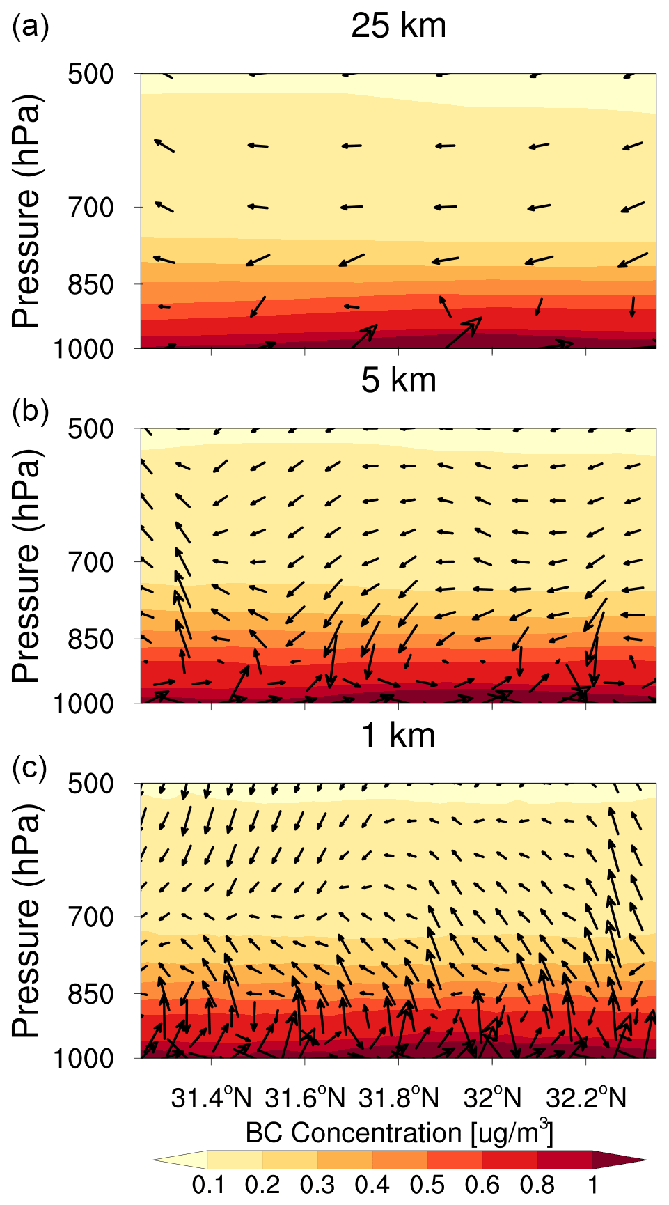
Figure 8 The latitude–pressure cross section of BC concentrations and wind speed flux along the USTC site for 25 km (a), 5 km (b), and 1 km (c) resolution simulations of the whole day. Vector arrows are the combination of wind speed fluxes v and w, with the vertical wind speed flux being multiplied by 100 for visibility. The shaded contours represent BC concentrations at each pressure level.

3.2.3 Impacts of land use type and terrain height on turbulent mixing coefficients at three different horizontal resolutions

Previous analyses indicate that the PBL mixing coefficient is one of the main factors contributing to the disparities in BC surface concentrations across multiple resolutions. Therefore, we further explored the factors influencing the spatial distribution of the PBL mixing coefficient. Our analysis reveals that the spatial distribution of the PBL mixing coefficient is closely related to land use types and terrain height. Specifically, the overall distribution of the turbulent mixing coefficient is closely resembled by the land use types (Figs. 1b and 7). However, in areas with obvious magnitude changes, such as east of the USTC site, the turbulent mixing coefficient displays distinct gradient changes that are not reflected in land use patterns. Notably, the spatial distribution of the topographic height (Fig. 1a) in this region exhibits distinct gradient changes similar to those of the turbulent mixing coefficients. Consequently, the spatial distribution of the turbulent mixing coefficient is influenced by both terrain and land use types. This correlation can be attributed to the interrelationship among turbulent mixing, friction velocity, terrain, and land use types. Terrain and land use types influence friction velocity by modifying surface roughness, which in turn directly affects turbulent mixing coefficients within the PBL. Higher surface roughness values typically lead to a greater fiction velocity, subsequently enhancing turbulent intensity and increasing the vertical mixing efficiency of pollutants within the PBL. To further investigate this relationship, the spatial distribution of the friction velocity is analyzed, as shown in Fig. 9. The analysis reveals that the friction velocity increases as the resolution increases from a 25 resolution to 5 and 1 km resolutions, with finer resolutions (5 and 1 km) capturing more spatial detail. Differences in friction velocity are illustrated in Fig. S15. The spatial distribution of the friction velocity indeed correlates with terrain and land use patterns, consequently influencing the distribution of the PBL mixing coefficient. As a result, the spatial distribution of the PBL mixing coefficient correlates with land use types and terrain height.

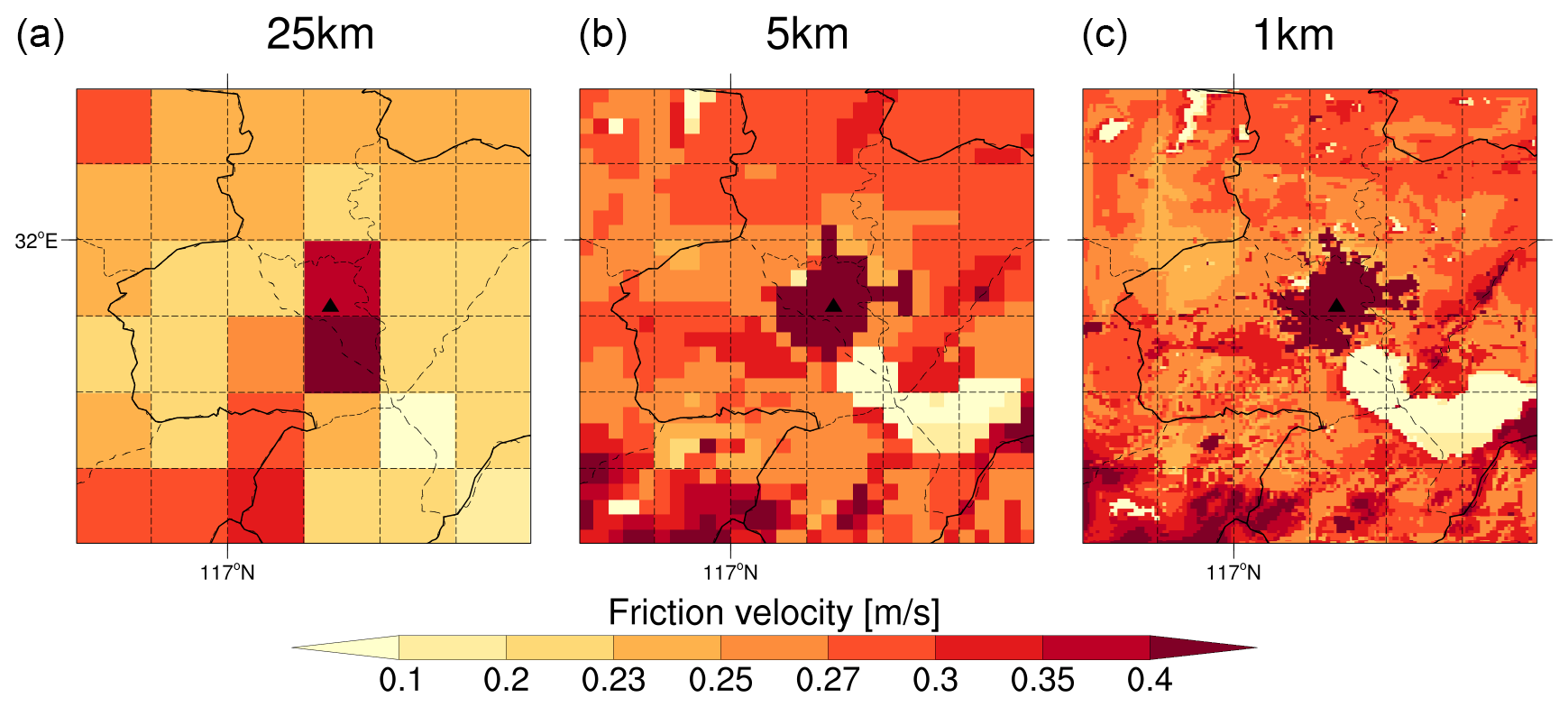
Figure 9 Spatial distribution of friction velocity in the study area for (a) 25 km, (b) 5 km, and (c) 1 km resolution simulations of the whole day. The solid black triangle indicates the location of the USTC site.

Our study indicates that variations in land use type distribution simulated at different horizontal resolutions are a significant factor causing changes in PBL mixing coefficients across multiple resolutions. These variations in mixing coefficients relate closely to BC surface concentrations, explaining specific patterns in BC surface concentration distributions. For example, the BC surface concentration south of the USTC site increases as resolution improves from 25 to 5 and 1 km resolutions (Figs. 4 and S8), contrasting with concentration variations simulated in other regions. Our analysis reveals that the turbulent mixing coefficient simulated at a 25 km resolution is higher compared to the two higher-resolution simulations in this area (Figs. 7 and S12). Moreover, the spatial distribution of land use types indicates that the 25 km resolution simulation resolves only a single urban land use type in this area (Fig. 1b). In contrast, higher-resolution simulations capture additional land use types beyond the urban, including lakes, farmland, and shrubs (Fig. 1b). The inclusion of these diverse land use types at a higher resolution leads to smaller PBL mixing coefficients in this area, as the surface roughness associated with lakes, farmland, and shrubs is generally lower than that of urban areas. As a result, the reduced vertical mixing in the finer-resolution (5 and 1 km) simulations results in higher BC surface concentrations south of the USTC site.

Additionally, to explore the differences in PBL mixing coefficients across multiple resolutions under uniform land use conditions, we designed another set of sensitivity experiments across three resolutions. As mentioned earlier, the only difference from the baseline experiment was the use of the default USGS land use classification data in the WRF model. As shown in Fig. S2, land use type data at different horizontal resolutions are approximately consistent in this setup. All other settings remained identical to those in the baseline experiment.

Figure 10 presents the spatial distribution of PBL mixing coefficients in the sensitivity experiment. Figure 10a illustrates the results across multiple resolutions averaged over the whole day. Similar to the baseline experiment, increasing resolution resolves more spatial detail. For example, in the area where the USTC site is located, the PBL mixing coefficient in the 25 km resolution simulation of the sensitivity experiment is approximately 4.3 m² s⁻¹, significantly lower than the 8 m² s⁻¹ observed in the baseline experiment. This pattern is consistent across higher resolutions (5 and 1 km). This finding aligns with the spatial distribution of land use types used in both sets of experiments (Figs. 1b and S2). The decrease in mixing coefficients in the sensitivity experiment stems from its land use data failing to resolve urban land types in urban areas. Figure 10b and c show the PBL mixing coefficients of the sensitivity experiment during daytime and nighttime, respectively. Consistent with the baseline experiment, the turbulent mixing coefficients during the day are substantially higher than at night. The PBL coefficients in the nighttime simulations are higher at 5 and 1 km resolutions compared to the 25 km resolution.

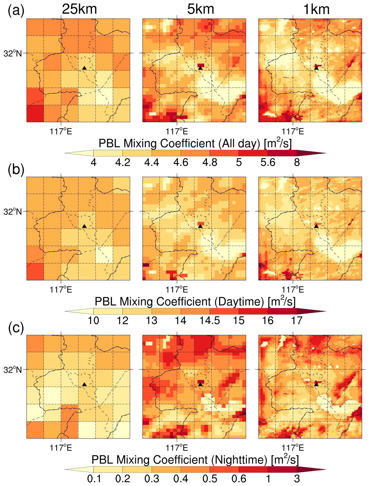
Figure 10 Spatial distribution of PBL mixing coefficients in the study area for (left) 25 km, (middle) 5 km, and (right) 1 km resolution simulations of (a) the whole day, (b) daytime, and (c) nighttime, respectively. The solid black triangle indicates the location of the USTC site. The simulation results are from the three sensitivity experiments.

Additionally, Fig. S16 further illustrates the differences in the parameterized PBL mixing coefficient between the 25 km resolution and the two higher-resolution simulations under roughly uniform land use conditions. Figure S16c shows that, in the city center, the boundary layer mixing coefficient parameterized at 5 and 1 km resolutions is higher than that at the 25 km resolution during nighttime. As urban areas are primarily flat, topographical differences between different resolutions in urban areas are minimal (almost negligible). Furthermore, because the land use types in the sensitivity experiment are approximately consistent across different resolutions, the main factor responsible for resolution-related differences in the PBL mixing coefficients in urban areas is the grid size. Notably, in areas with significant topographic variations, such as suburban and rural regions, the difference in boundary layer mixing coefficients between 25 and 5 km/1 km resolutions in the sensitivity experiment strongly correlates with the spatial distribution of topographic differences. This directly demonstrates that topographic height is also a key determinant of the boundary layer mixing coefficient distribution. Qian et al. (2010) indicated that the terrain affects the transport and mixing of aerosols and trace gases, as well as their concentrations across multiple resolutions, through its impact on meteorological fields such as wind and the PBL structure. These terrain-related effects are particularly significant in regions with more variable topography. Additionally, Fig. S17 shows that the turbulent mixing intensity parameterized at a 5 km resolution in the sensitivity experiment is greater than that at a 1 km resolution. Further analysis of the latitude–pressure cross section of BC concentrations and vertical wind speed flux, as shown in Fig. S18, indicates that, similar to the baseline experiment, the 1 km resolution of the sensitivity experiment resolves more small-scale turbulent eddies, capturing more prominent vertical wind speed flux, thus resulting in stronger turbulent mixing.

Through comprehensive analysis of both baseline and sensitivity experiments, we found that, within the resolution range of 25 to 1 km, the spatial distribution accuracy of land use types plays a decisive role in parameterizing the PBL mixing coefficient. Finer land use type information at higher resolutions directly alters the spatial distribution of the boundary layer mixing coefficient, with urban surfaces significantly increasing the parameterized PBL mixing coefficient. Therefore, accurately representing land use types, particularly urban surfaces, is critical for parameterizing the PBL mixing coefficient. On the other hand, in the sensitivity experiment, areas of complex terrain with significant elevation (such as suburban, rural, and hilly regions) increase mixing coefficients by enhancing surface roughness, whereas this effect is weaker in flat urban areas. Consequently, differences in PBL mixing coefficients across multiple resolutions strongly correlate with terrain precision. Higher resolutions can resolve finer terrain variations, affecting local turbulent mixing (such as terrain-induced mechanical turbulence). This confirms the dominant role of high-resolution terrain and land use information in PBL mixing coefficient parameterization. Notably, in regions where land use types and terrain height remain relatively flat and consistent across different horizontal resolutions in the sensitivity experiments, increasing resolution still leads to enhanced boundary layer mixing coefficients, highlighting the importance of the grid size with respect to parameterizing the boundary layer mixing coefficient. In the resolution range from 5 to 1 km, higher resolution slightly reduces the parameterized boundary layer mixing coefficient. However, the 1 km resolution model resolves more small-scale turbulent eddies, resulting in stronger turbulent mixing at night. In summary, for parameterization of boundary layer mixing coefficients across multiple resolutions, high-resolution surface information is more important in regions with significant changes in land use type and terrain height. Grid size is also crucial in regions with more gradual changes, where higher-resolution grids consistently enhance the boundary layer mixing representation. Therefore, to improve PBL mixing coefficient simulation, priority should be given to ensuring the accuracy of land use data (especially the spatial representation of urban types), precise terrain representation in complex regions, and appropriate grid resolution to enhance turbulent mixing simulation.

3.3 Simulated BC column concentrations and impacts of turbulent mixing at various horizontal resolutions

3.3.1 Simulated BC column concentrations at three different horizontal resolutions

It is generally accepted that the turbulent mixing process primarily affects pollutant surface concentrations by mixing surface pollutants into higher layers, without altering the column concentration. However, in this study, BC column concentrations exhibit differences across multiple-resolution simulations. Therefore, we further investigate the spatial distribution of BC column concentrations and the main mechanisms behind these variations. Figure 11a illustrates the spatial distribution of BC column concentrations simulated at three resolutions, averaged over the whole day. The regional average values for the three resolutions are 2041, 2150, and 2223 µg m⁻², respectively. The 5 and 1 km resolution simulations yield larger BC column concentrations compared to 25 km resolution simulations. The spatial distribution of BC column concentrations simulated at a 25 km resolution is highly consistent with the BC emission distributions (Fig. 2), showing high concentrations in central urban areas exceeding 2500 µg m⁻², while regions distant from urban centers demonstrate lower concentrations, generally below 2100 µg m⁻². The 5 km resolution simulation results indicate peak column concentrations concentrated in urban areas and spread around, with the southwestern area approaching 2250 µg m⁻². The 1 km resolution simulation results yield the largest BC column concentrations and demonstrate the most pronounced diffusion tendency, with most areas exceeding 2250 µg m⁻². Figure 11b and c reveal lower BC column concentrations during the daytime compared to those at night, with a more pronounced dispersion trend of column concentrations simulated at night. Figure S19 depicts the differences in BC column concentrations between the 25 and 5 km resolutions and between the 25 and 1 km resolutions, revealing that BC column concentrations at coarser resolutions are marginally lower than those at finer resolutions (5 and 1 km) in most of the study areas. On the other hand, the BC column concentration simulated at a 1 km resolution are larger than those at a 5 km resolution, as shown in Fig. S20. In conclusion, BC column concentrations increases with a higher resolution, accompanied by a more pronounced dispersion tendency towards higher and farther areas.

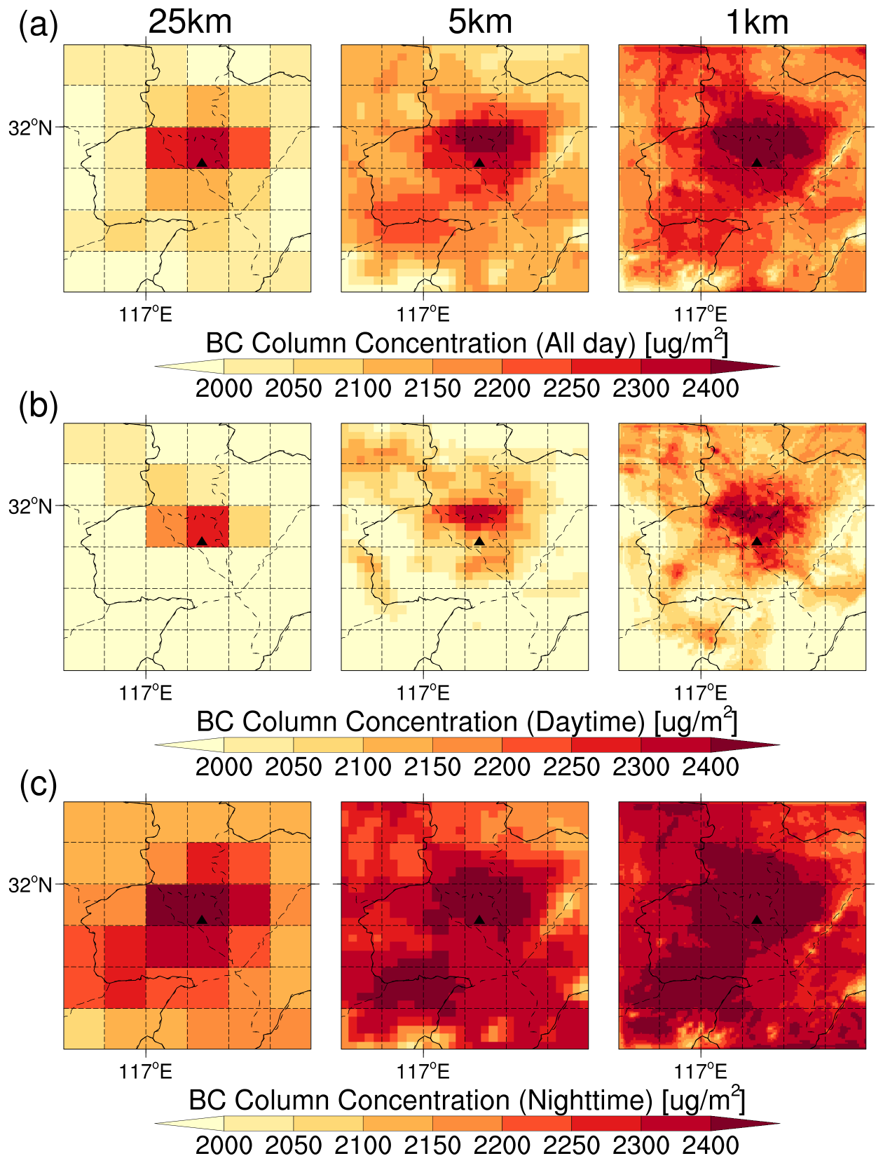
Figure 11 Spatial distribution of the BC column concentration in the study area for (left) 25 km, (middle) 5 km, and (right) 1 km resolution simulations of (a) the whole day, (b) daytime, and (c) nighttime, respectively. The solid black triangle indicates the location of the USTC site.

3.3.2 Impacts of turbulent mixing on BC column concentrations at three different horizontal resolutions

We further analyze the mechanisms underlying the differences in BC column concentrations across multiple resolutions in urban areas. Figure 12a displays the vertical profiles of BC concentrations averaged over the study area. The BC profiles at a 25 km resolution exhibit significant variability, generally decreasing from the surface to higher altitudes. The near-surface BC concentration is approximately 3 times higher than those at high altitudes, with surface concentrations reaching about 3 µg m⁻³. At an altitude of 100 m, the concentration drops to 1 µg m⁻³, while above this elevation, the BC concentration is less than 1 µg m⁻³. Substantial disparities exist among multiple-resolution simulations with respect to the vertical profiles of BC concentrations. Our analyses above have shown that, near the surface, the parameterized mixing coefficients and directly resolved vertical wind speed flux are lower at 25 km resolution compared to at 5 and 1 km resolutions, reducing the vertical mixing of pollutants in 25 km resolution simulations. Thus, BC concentrations at a 25 km resolution are higher near the surface and lower at higher altitudes compared to values from high-resolution (5 and 1 km) simulations. Moreover, the parameterized PBL mixing coefficient at a 1 km resolution is lower than at a 5 km resolution in the atmosphere, but the directly resolved upward vertical wind speed flux by the model dynamic process reaches higher altitudes at a 1 km resolution compared to a 5 km resolution. Thus, due to the combined effects of these two processes, the intensity of turbulent mixing is similar between the 5 and 1 km resolutions at near-surface levels, whereas it is greater at a 1 km resolution than at a 5 km resolution at higher altitudes. In numerical models, sub-grid-scale (SGS) turbulent diffusion is typically simulated by parameterization schemes. However, as the model resolution increases, such as achieving a 1 km resolution, the turbulent mixing is increasingly resolved by the dynamical framework of the model. This advancement allows the model to capture dynamic structures and small-scale turbulence more accurately, significantly enhancing the strength of turbulent mixing. The resolution of dynamic processes reduces the reliance on traditional parameterization schemes, thereby decreasing the PBL mixing coefficient parameterized at finer resolutions. In conclusion, at higher altitudes, the enhanced turbulent mixing efficiently facilitates more ground-emitted pollutants to a higher height as the resolution increases. Thus, BC concentrations at resolutions of 5 and 1 km are similar near surface, with a 1 km resolution yielding the largest concentrations at higher altitudes.

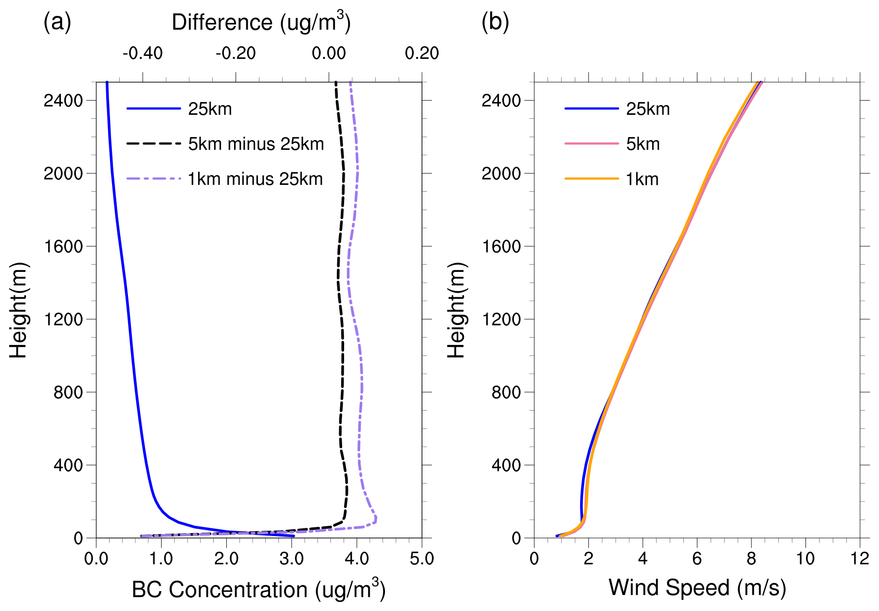
Figure 12 (a) Vertical profiles of BC concentrations simulated at a 25 km resolution (solid blue line), the difference between resolutions of 5 and 25 km (dashed black line), and the difference between resolutions of 1 and 25 km (dashed purple line) averaged over the study area for the whole day, respectively. (b) Vertical profiles of wind speed simulated at a 25 km resolution (solid blue line), 5 km resolution (solid pink line), and 1 km resolution (solid orange line) averaged over the study area for the whole day, respectively.

To further investigate the BC column concentrations and their dispersion tendency towards farther areas, we analyzed the vertical profile of wind speed at three resolutions averaged over the study area, as shown in Fig. 12b. The vertical profile of wind speed is relatively consistent across the three resolutions. From the ground to higher altitudes, the overall wind speed gradually increases, transitioning from low speeds near the surface to higher speeds aloft. Near the ground, the simulated average wind speed is approximately 1 m s⁻¹, increasing to 4 m s⁻¹ at an altitude of 1 km and reaching an average of about 7 m s⁻¹ at an altitude of 2 km. In the upper atmosphere, characterized by higher wind speeds, pollutants mixed up from near the surface can be transported and dispersed farther. As previously mentioned, BC simulated in higher-resolution simulations can be transported to higher altitudes, thus dispersing over greater distances due to stronger winds. Therefore, as the resolution increases, the trend of diffusion towards farther regions in the simulated BC column concentrations becomes more pronounced.

As previously discussed, higher-resolution simulations facilitate BC transport to greater altitudes and further distances. This phenomenon extends its atmospheric lifetime, consequently resulting in increased column concentrations. Bauer et al. (2013) noted that turbulent mixing and convective transport processes play a critical role in determining BC lifetimes. Figure 13 illustrates the spatial distribution of BC lifetime, calculated by dividing the BC column concentration by the dry deposition flux. It demonstrates that the BC lifetime gradually lengthens as the resolution increases. The average lifetime of BC column concentrations in the study area is 344, 350, and 382 h for 25, 5, and 1 km resolutions, respectively. These results clearly demonstrate that BC simulated at higher resolutions exhibits prolonged atmospheric residence times. Consequently, the BC column concentration is higher for high-resolution simulations.

Figure 13 Spatial distribution of the BC lifetime in the study area for (a) 25 km, (b) 5 km, and (c) 1 km resolution simulations of the whole day, respectively. The solid black triangle indicates the location of the USTC site.

4 Conclusion and discussion

Turbulent mixing plays a crucial role in urban pollutant transport by enhancing the diffusion of atmospheric pollutants. Current atmospheric models often underestimate turbulent exchange within stable nocturnal boundary layers, and the turbulent mixing varies markedly across different model horizontal resolutions. However, few studies have analyzed how turbulent mixing processes across multiple resolutions affect pollutant concentrations in urban areas. Therefore, our goal is to elucidate the variations in pollutant concentrations across multiple resolutions and investigate the influence of turbulent mixing on pollutant concentrations at various resolutions.

We conducted a WRF-Chem simulation nested at three resolutions (25, 5, and 1 km) in the Hefei area. BC surface concentrations decrease as resolution increases from 25 to 5 km and further to 1 km but are similar at 5 and 1 km resolutions, showing significant diurnal variations with higher concentrations at night and lower concentrations during the daytime. The BC surface concentrations across multiple resolutions align well with USTC site observations during daytime but are overestimated at night, with this overestimation decreasing at higher resolution (5 and 1 km). Disparities in BC surface concentrations between the two finer-resolution simulations and the 25 km resolution simulation are primarily attributable to nocturnal concentrations. In addition, the diurnal variation in the PM_2.5 surface concentrations simulated at different resolutions follows the same trend as the observed concentrations at the national monitoring sites, with a slight underestimation during daytime and an overestimation at night. The PBL mixing coefficient plays a crucial role in controlling surface particulate matter concentrations at night. Larger nighttime PBL mixing coefficients and a higher vertical wind speed flux at 5 and 1 km resolutions compared to a 25 km resolution near the surface result in lower BC surface concentrations. However, the PBL mixing coefficient at a 5 km resolution is larger than at a 1 km resolution. Moreover, the upward vertical wind speed flux resolved at a 1 km resolution reaches higher altitudes compared to that at 25 and 5 km resolutions, indicating more small-scale eddies and resulting in enhanced turbulent mixing. Consequently, near the surface, the combined effects of the parameterized PBL mixing coefficient and the directly resolved vertical wind speed flux lead to similar BC surface concentrations at 5 and 1 km resolutions.

Further analysis reveals that the spatial distribution of PBL mixing coefficients is influenced by both land use types and terrain heights. The turbulent mixing coefficient correlates with the spatial distribution of land use types at smaller scales, with urban underlying surfaces notably increasing the parameterized PBL mixing coefficient. The mixing coefficient also strongly correlates with terrain heights at larger scales, particularly in regions with complex topography and significant elevation differences, where higher terrain substantially enhances mixing coefficients. This correlation can be attributed to the interrelationship among turbulent mixing coefficients, friction velocity, terrain, and land use types. The static database of terrain and land use types employed as model input determines the surface roughness. Higher surface roughness typically leads to greater fiction velocity, subsequently increasing the PBL mixing coefficients. Moreover, in regions where land use types and terrain height remain relatively flat and consistent across multiple resolutions, increasing resolution still enhances boundary layer mixing coefficients, highlighting the importance of grid size. Thus, both surface information and grid resolution are crucial for accurately parameterizing PBL mixing coefficients, with priority given to accurate land use data, precise terrain representation, and higher grid resolution to improve turbulent mixing simulations.

In WRF-Chem, the mixing coefficients of chemical species are clipped to empirically chosen thresholds of 1 m² s⁻¹ over rural areas and 2 m² s⁻¹ over urban areas to prevent unrealistically low values. These thresholds are modified based on differences in anthropogenic CO and primary PM_2.5 emissions between rural and urban regions. Importantly, this adjustment applies exclusively to gases and not to aerosols when the MOSAIC or MADE/SORGAM aerosol schemes are used. This is because the adjustment does not couple with the aerosol PBL mixing scheme in WRF-Chem, although potential modifications could be made for compatibility with the MOSAIC or MADE/SORGAM scheme. Thus, the boundary layer mixing coefficient for gases is implicitly influenced by emission resolution rather than directly controlled by model resolution. In this study, this treatment caused gas mixing coefficients to converge across different horizontal resolutions, preventing us from accurately assessing the impact of horizontal resolution on gas turbulent mixing. For aerosols, however, the original PBL mixing coefficients are retained, which are directly parameterized from boundary layer parameterization schemes. Therefore, our focus is mainly on particulate matter in this analysis, and we omitted this modification for gases.

The variations in turbulent mixing across multiple-resolution simulations not only affect the BC surface concentration but also lead to different BC column concentrations. BC column concentrations increase with improved resolution, accompanied by a more pronounced diffusion tendency towards higher altitudes and distant regions. Throughout the atmosphere, turbulent mixing intensifies with improved resolution, resulting in pollutants being transported to higher altitudes. Concurrently, wind speed increases with altitude, facilitating the pollutants which are mixed to higher altitudes to be spread farther. Consequently, BC simulated at a higher resolution is transported to greater altitudes and dispersed to farther regions, thus persisting in the atmosphere for longer periods and leading to longer lifetimes. As a result, BC column concentrations increase with finer resolutions.

This study highlights the importance of model horizontal resolution in simulating the dispersion of atmospheric pollutants. We observed that the enhanced turbulent mixing strength at high resolution can more accurately reproduce the vertical and horizontal distribution of pollutants, thus aligning the simulated pollutant surface concentrations more closely with actual observations. In contrast, turbulent mixing in low-resolution simulations, primarily depending on boundary layer parameterizations, may not adequately capture the dynamics of turbulence, leading to discrepancies between the simulated and actual distribution of pollutants, particularly under stable boundary conditions at night. Future research should focus on improving PBL parameterization schemes to enhance model performance at lower resolutions, thereby better serving the needs of air pollution control and environmental management.

We have noted that the parameterized PBL mixing coefficient decreases when transitioning from 5 to 1 km resolution, alongside an increase in the vertical wind speed flux which represents turbulent mixing directly resolved by the dynamical processes. This trend suggests that if the resolution was further increased to large-eddy simulation (LES) scales, the parameterized PBL mixing coefficient might diminish significantly, potentially approaching zero, while the turbulence mixing resolved directly by the dynamics would intensify considerably. At LES scales, the majority of turbulent mixing is directly resolved, capturing the atmospheric dynamical processes and turbulent exchanges more realistically, thereby reducing the simulation biases caused by parameterization errors. This shift diminishes reliance on traditional boundary layer parameterizations to simulate turbulent mixing, leading to a substantial reduction in the parameterized boundary layer mixing coefficient. By capturing the finer details of atmospheric dynamics, the model provides a more realistic representation of turbulent mixing and related physical processes, which is crucial for understanding weather patterns, climate variability, and pollutant dispersion. However, due to the huge computational resources required for LES, we have not yet performed an analysis at the LES scale, but it is worth further exploring in the future.

Moreover, in addition to the influence of surface roughness on turbulence intensity, surface type significantly affects the CBL and turbulence mixing strength through differences in radiative flux absorption, reflection, and heat exchange. There are substantial variations in the absorption and reflection of SW radiation across different surface types. Urban areas typically have lower albedo, absorbing more SW radiation, which increases surface temperature and transfers energy to the atmosphere as sensible heat. In contrast, vegetated areas generally have higher albedo and, through transpiration, release more latent heat while reducing sensible heat output. These differences in energy exchange between the surface and atmosphere directly influence turbulence strength. Furthermore, the varying balance between sensible and latent heat fluxes across different surface types impacts turbulence intensity and CBL depth. For instance, urban areas, with stronger sensible heat flux, tend to generate more intense thermal convection, often resulting in a shallower CBL, while vegetated areas, with predominant latent heat flux, may develop more stable atmospheric conditions, potentially leading to a deeper CBL with weaker turbulence. These mechanisms of radiative absorption and heat exchange are crucial in the formation of the diurnal CBL and determining turbulence intensity. Future studies on land use impacts on turbulence mixing should therefore consider not only surface roughness but also radiative flux differences, sensible and latent heat exchange mechanisms, and the comprehensive effects of surface albedo on turbulence development.

Our analysis also found that a higher resolution facilitates transport over greater distances, suggesting that intercity pollutant diffusion can be affected by model resolution, with a coarse resolution potentially reducing long-range transport and interurban impacts. While previous studies have examined pollutant formation mechanisms at specific resolutions and explored the physical and chemical interactions among megacities, few have considered the impacts of different resolutions on long-range transport between cities. Due to computational cost constraints, interurban impacts are not discussed in this study, but they deserve further investigation in the future. Finally, while vertical resolution is held constant in our study, we recognize that it could influence the interpretation of the turbulence processes in certain scenarios, especially in regions with complex vertical structures. Therefore, future work could systematically explore the interplay between vertical resolution and pollutant concentration or aerosol–boundary layer feedbacks.