State-wide California 2020 carbon dioxide budget estimated with OCO-2 and OCO-3 satellite data

Satellite observations are instrumental in observing spatiotemporal variability in carbon dioxide (CO₂) concentrations, which can be used to derive fluxes of this greenhouse gas. This study leverages NASA's Orbiting Carbon Observatory-2 and -3 (OCO-2 and OCO-3, respectively) CO₂ observations with a Gaussian process (GP) machine learning inverse model, a Bayesian nonparametric approach well suited for integrating the unique spatiotemporal characteristics of these satellite observations, to estimate subregional CO₂ fluxes. Utilizing the GEOS-Chem chemical transport model (CTM) to simulate column-average CO₂ concentrations (XCO₂) for 2020 in California – a period marked by the coronavirus disease (COVID-19) pandemic, drought conditions, and significant wildfire activity – we estimated the state-wide CO₂ emission rates constrained by OCO-2/3. This study developed prior fossil fuel emissions to reflect reduced activities during the COVID-19 pandemic, while net ecosystem exchange (NEE) and fire emissions were derived based on satellite data. GEOS-Chem source-specific XCO₂ concentrations for fossil fuels, NEE, fire, and oceanic sources were simulated coincident to OCO-2/3 XCO₂ retrievals to estimate state-wide sector-specific and total CO₂ emissions. GP inverse model results suggest that annual posterior median fossil fuel emissions were consistent with prior estimates (317.8 and 338.4 Tg CO₂ yr⁻¹, respectively; 95 % confidence level) and that posterior NEE fluxes had less carbon uptake compared to prior fluxes (−36.8 vs. −99.2 Tg CO₂ yr⁻¹, respectively; 95 % confidence level). Posterior fire CO₂ emissions were estimated to be 68.0 Tg CO₂ yr⁻¹, which was much lower than a priori estimates (103.3 Tg CO₂ yr⁻¹). The total median annual CO₂ emissions for the state of California in 2020 were estimated to be 349.6 Tg CO₂ yr⁻¹ (range of 272.8–428.6 Tg CO₂ yr⁻¹; 95 % confidence level), aligning closely with the prior total estimate of 342.5 Tg CO₂ yr⁻¹. This study, for the first time, demonstrates that OCO-2/3 XCO₂ observations can be assimilated into inverse models to estimate state-wide source-specific CO₂ fluxes on a seasonal and annual scale.

1 Introduction

Carbon dioxide (CO₂) is the most abundant greenhouse gas in Earth's atmosphere and contributes predominantly to the present-day increase in global radiative forcing (Dunn et al., 2022). Due primarily to anthropogenic emissions from fossil fuel production and usage, global concentrations of CO₂ have nearly doubled since the beginning of the preindustrial era (Gulev et al., 2021; Lan et al., 2023). A recent comprehensive budget analysis of global CO₂ fluxes suggests that, as of 2022, anthropogenic emissions are ∼ 10 Gt C yr⁻¹ (primarily from combustion of coal, oil, and natural gas) with an oceanic and terrestrial uptake offset of ∼ 3 Gt C yr⁻¹ and ∼ 4 Gt C yr⁻¹, respectively (Friedlingstein et al., 2023). According to this report, the United States (US) contributes 14 % (∼ 1.4 Gt C yr⁻¹) of global CO₂ anthropogenic emissions. The sectors contributing the most to US anthropogenic emissions are transportation, electricity generation, and industry (United States Environmental Protection Agency, 2023). One of the larger emitters of greenhouse gases in the US is the state of California which, as of 2021, contributes ∼ 0.1 Gt C yr⁻¹ of CO₂ (CARB, 2023). In 2006, the state of California passed Assembly Bill 32 (AB 32) which required that the state's greenhouse gas emissions must be reduced to 1990 levels by the year 2020. California was able to achieve this goal, but in order to demonstrate this, as well as the success of other future emission reduction goals, it is vital to have accurate estimates of past and present-day greenhouse gas emissions.

Bottom-up inventories of CO₂ are commonly used to derive country-level to state-wide fossil fuel anthropogenic emissions in the US (e.g., Andres et al., 2012; CARB, 2023). Calculations of natural sources and sinks (e.g., terrestrial and marine biosphere and wildfires) contributing to total CO₂ emissions are frequently estimated using model predictions (Friedlingstein et al., 2023). The California Air Resources Board (CARB) has quantified state-wide greenhouse gas emissions for California between 2000–2021 (CARB, 2023). Anthropogenic and natural bottom-up CO₂ flux estimates are typically implemented in atmospheric transport models and compared to atmospheric observations in order to assess their accuracy. In situ observations of CO₂ from ground-based, tower, and aircraft platforms, due to their high accuracy and precision, are most frequently used to evaluate the quality of these emission estimates (Graven et al., 2018; Cui et al., 2022). While highly accurate, these types of in situ observations are limited in their spatiotemporal coverage and ability to constrain large regions and annual cycles of emissions. The assimilation of the satellite-retrieved column-averaged dry-air mole fraction of CO₂ (XCO₂) (e.g., Orbiting Carbon Observatory-2, OCO-2; Orbiting Carbon Observatory-3, OCO-3; Greenhouse Gases Observing Satellite, GOSAT; GOSAT-2; Carbon Dioxide Monitoring constellation, CO₂M; TanSat) into atmospheric transport models has been demonstrated to be able to constrain emissions on a global- to country-level scale more effectively in regions which lack dense in situ measurement networks (Pandey et al., 2016; Yang et al., 2021; Peiro et al., 2022; Philip et al., 2022; Imasu et al., 2023; Byrne et al., 2023; Noël et al., 2024). This study focuses on CO₂ fluxes in the state of California, where OCO-2 and OCO-3 have been used to constrain urban-scale emissions in the megacity of Los Angeles (Hedelius et al., 2018; Ye et al., 2020; Kiel et al., 2021; Wu et al., 2022; Roten et al., 2023; Hamilton et al., 2024). However, to date, no studies have demonstrated the capability to evaluate and constrain CO₂ fluxes using satellite-retrieved information on a state-wide spatial domain such as California. For California and other states, this is important, as some state agencies only release state-wide inventories (not specifically for urban areas), and many climate programs are generated based on the state-wide inventories.

While satellite-based atmospheric inverse modeling provides a significantly enhanced method for quantifying CO₂ emissions, using satellite observations in atmospheric inversions introduces two principal challenges: (1) incorporating the spatiotemporal covariance inherent in satellite data and (2) accurately estimating the hyperparameters (such as the length scale) of this covariance. Satellite observations contain both spatial and temporal properties, meaning that the data have inherent spatial and temporal characteristics that inform us about surface emissions. However, numerous inverse modeling studies have not consistently incorporated both covariance structures (Johnson et al., 2016; Fischer et al., 2017; Cui et al., 2019; Graven et al., 2018; Nathan et al., 2018; Ye et al., 2020; Wu et al., 2022; Roten et al., 2023). While some studies have accounted for both spatial and temporal covariances, they have not determined the optimal hyperparameters that align with the satellite observations (e.g., Turner et al., 2020). For example, the length scale parameter is crucial for influencing the covariance, which in turn affects the estimation of the unknown functions; in many cases, however, this parameter is not estimated explicitly for its optimal value but instead prescribed. In this study, we applied an atmospheric inversion system which fully utilizes the spatiotemporal properties embedded in satellite data (i.e., OCO-2 and OCO-3). This system is built based on the Gaussian process (GP) machine learning (ML) approach enabled by modern probabilistic programming languages (PPLs). GP is an ML technique that treats predictions as distributions, rather than single points, providing a measure of prediction uncertainty; this is ideal for atmospheric inverse modeling (see Sect. 2.4), as posterior uncertainties are vital for providing quantitative information on the confidence level of the emission constraint. Inversion CO₂ models, other than analytical systems, cannot always provide posterior emission uncertainties, and these estimates can be unreliable and computationally expensive to calculate (e.g., Liu et al., 2014; Bousserez et al., 2015). The kernels (i.e., covariance functions) of GP models are employed to capture the intricate spatiotemporal correlation structures of OCO-2/3 data. PPLs have been used in previous studies (e.g., Jeong et al., 2017, 2018), but modern PPLs provide significantly improved capabilities to implement GP models. Specifically, the built-in functions for GP kernels in modern PPLs enhance our ability to model the covariance structure of OCO-2/3 data.

This study applies inverse modeling techniques following the GP/ML methods described in further detail in Sect. 2.4 to estimate CO₂ fluxes in California for the full year of 2020 using XCO₂ observations from OCO-2 and OCO-3. The year 2020 had numerous anomalous features likely impacting total CO₂ fluxes in California, such as reduced anthropogenic emissions caused by coronavirus disease pandemic (COVID-19) lockdown procedures (Yañez et al., 2022), extreme wildfire activity (Jerret et al., 2022; Safford et al., 2022), and drought conditions (Steel et al., 2022). The impact that these types of events have on CO₂ fluxes are challenging to predict and difficult to replicate in bottom-up emission inventories. This study is structured as follows: Sect. 2 presents the forward and inverse models, satellite observations, and bottom-up emission inventories; Sect. 3 discusses the results of the study; and Sect. 4 contains the discussion and conclusions.

2 Methods

2.1 GEOS-Chem forward model

The forward model used to calculate atmospheric concentrations of CO₂ corresponding to OCO-2 and OCO-3 observations was the GEOS-Chem (version 14.0.1) chemical transport model (CTM) (Bey et al., 2001; Nassar et al., 2010). GEOS-Chem was used to simulate XCO₂ concentrations corresponding to each OCO-2 and OCO-3 retrieval for a nested North American domain (10–70° N, 40–140° W) driven by Modern-Era Retrospective Analysis for Research and Applications, Version 2 (MERRA-2) meteorology at a 0.5° × 0.625° spatial resolution using 47 vertical levels from the surface to 0.01 mbar. Chemical boundary conditions (BCs) of CO₂ used in the nested simulations were provided by a global GEOS-Chem-based 4D-Var data assimilation system that was run at a 4.0° × 5.0° horizontal spatial resolution using 47 vertical levels. These global simulations of CO₂ for the year 2020 were constrained using inverse model methods through the assimilation of OCO-2 XCO₂ land nadir + land glint (LN + LG) retrievals and global in situ observations (Philip et al., 2019, 2022). The bottom-up emission inventories for CO₂ fluxes from fossil fuel (FF), net ecosystem exchange (NEE), wildfires, and oceans are described in Sect. 2.2. GEOS-Chem was initialized with chemical BCs and run for the entire year of 2020 with 2 months of spin-up time.

Total atmospheric CO₂ and source-apportioned (i.e., FF, NEE, fire, ocean, and boundary conditions) concentrations were calculated over California for all OCO-2 and OCO-3 observations. These source-attributed concentrations were calculated with sensitivity simulations by turning off individual source fluxes or boundary conditions and comparing these results to the total atmospheric CO₂ concentration predictions from simulations with all sources included. Model-simulated XCO₂ corresponding to each OCO-2 and OCO-3 retrieval (H) were derived through the convolution of model CO₂ profiles with the column averaging kernel vector (a) from OCO-2 and OCO-3 following Eq. (1):

$$\begin{array}{}\text{(1)}& H=X{{\mathrm{CO}}_{\mathrm{2}}}_a+{\mathit{a}}^T(\mathit{f}\left(\mathit{\sigma }\left(\mathit{x}\right)\right)-{\mathit{c}}_a),\end{array}$$

where prior profiles of CO₂ (c_a) and prior column CO${}_{\mathrm{2}}\left(X{\mathrm{CO}}_{{\mathrm{2}}_a}\right)$ represent prior information used in the OCO-2 and OCO-3 XCO₂ retrieval (O'Dell et al., 2012) and f(σ(x)) represents the GEOS-Chem-predicted vertical profiles of CO₂ interpolated to the retrieval levels of OCO-2 and OCO-3.

2.2 Bottom-up emission inventories

Bottom-up emission inventories used to drive GEOS-Chem simulations are described in Table 1, and seasonally averaged emission maps are displayed in Fig. S1 in the Supplement. The Vulcan version 3.0 FF emission inventory covers all anthropogenic source sectors of CO₂ in California (i.e., residential, commercial, industrial, electricity production, on-road, non-road, commercial marine vessel, airport, rail, and cement) between 2010–2015 (Gurney et al., 2020a). To create a spatially and temporally resolved Vulcan inventory in California for the year 2020 (V2020_M), the hourly 2015 Vulcan emissions (V2015_M) are scaled by an annual and a monthly scaling factor using Eq. (2). The sector-specific annual scaling factor ($R_{\mathrm{2020}/\mathrm{2015}}^{\mathrm{CARB}}$) was calculated as the ratio of annual emissions from that sector in the CARB inventory for 2020 (which accounts for COVID-19 lockdown emission reductions; CARB, 2022) to the 2015 emissions. The sector-specific monthly scaling factor (R_M) was calculated from activity data from each sector, as the ratio of monthly activity to annual average activity, and used to appropriately distribute reductions due to the COVID-19 lockdown throughout the year.

$$\begin{array}{}\text{(2)}& V{\mathrm{2020}}_{\mathrm{M}}=V{\mathrm{2015}}_{\mathrm{M}}\times R_{\mathrm{2020}/\mathrm{2015}}^{\mathrm{CARB}}\times R_{\mathrm{M}}\end{array}$$

The Vulcan inventory for 2015 was then multiplied by these scaling factors to produce V2020_M. Both Vulcan and CARB provide the same sector-level emission estimates, so the scaling was done for each emission sector separately. The scaled 2020 Vulcan inventory was then aggregated to 0.1° × 0.1° (latitude × longitude).

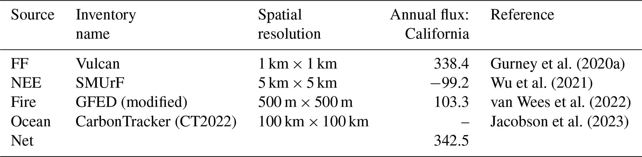
Table 1 Bottom-up prior CO₂ emission inventories and the 2020 terrestrial carbon budget (Tg CO₂ yr⁻¹) for California.

Natural CO₂ emission source (NEE, wildfire, and ocean) estimates were available for the year 2020, and no scaling was necessary. Biospheric fluxes of CO₂ were derived using monthly 5 km × 5 km NEE calculations from the Solar-Induced Fluorescence for Modeling Urban biogenic Fluxes version 1 (SMUrF v1; Wu et al., 2021) model. SMUrF calculates gross primary production (GPP), respiration (R_eco), and NEE (= R_eco – GPP) fluxes using (1) land cover type 500 m MODerate resolution Imaging Spectroradiometer (MODIS) data, (2) solar-induced fluorescence (SIF) from the OCO-2 sensor, (3) aboveground biomass at a 100 m resolution from GlobBiomass, (4) observed flux measurements from eddy-covariance towers, and (5) gridded soil and air temperature data products. Wildfire CO₂ emissions were implemented using a modified Global Fire Emissions Database version 4 (GFED4) dataset (van Wees et al., 2022). This modified version of GFED4 was produced using MODIS burned area and fire detection data with a spatial resolution of 500 m. Finally, oceanic CO₂ fluxes were derived from CarbonTracker (CT2022; Jacobson et al., 2023) 1° × 1° output. These CT2022 coarse-spatial-scale fluxes were interpolated to match the GEOS-Chem model spatial resolution.

2.3 OCO-2 and OCO-3 observations

NASA has two operational satellites with the spatial resolution and precision necessary to constrain point-source to regional- and global-scale CO₂ emissions (i.e., OCO-2 and OCO-3). OCO-2 was launched in 2014 and is a Sun-synchronous polar-orbiting satellite which is in the Afternoon Constellation (A-train) of Earth observing satellites with a local overpass time of ∼ 13:30 LT (local time) retrieving XCO₂ at a 1.3 km × 2.3 km spatial resolution (Crisp et al., 2017). OCO-3 has been aboard the International Space Station (ISS) since 2019 and has an orbital inclination of 51.6°, providing observations at varying times of the day (Eldering et al., 2019). OCO-3 makes orbital observations; however, it differs from OCO-2, as it has the capability to make snapshot area maps (SAMs) which cover 80 km × 80 km at the native spatial resolution of 1.6 km × 2.2 km. The XCO₂ retrievals from OCO-2 and OCO-3 both use the Atmospheric Carbon Observations from Space (ACOS) algorithm (O'Dell et al., 2018), and this study applied version 11r and version 10.4r of OCO-2 and OCO-3, respectively. Retrievals of XCO₂ from the LN + LG retrieval modes were used for comparison to GEOS-Chem and to estimate posterior state-wide CO₂ emissions. As individual high-spatiotemporal-resolution OCO-2 and OCO-3 retrievals do not provide independent pieces of information, they are averaged to the 0.5° × 0.625° spatial resolution of GEOS-Chem in this study. In total, 1614 co-located model–satellite data points were available during 2020 to evaluate prior XCO₂ predictions and constrain posterior CO₂ emissions. The seasonal distribution (meteorological seasons: winter – December, January, and February – DJF; spring – March, April, and May – MAM; summer – June, July, and August – JJA; fall – September, October, and November – SON) of these co-locations was as follows: 386, 299, 551, and 378 for the winter, spring, summer, and fall months, respectively. The spatial distribution of the observational coverage provided by OCO-2 + OCO-3 during 2020 is displayed in Fig. S2.

2.4 Inverse model technique

The inverse model developed for this study used a GP/ML framework. GP is a flexible, nonparametric approach, distinguished by its use of hyperparameters, that defines a prior probability distribution over functions (Williams and Rasmussen, 2006; Biship, 2007; Murphy, 2022). A GP is fully characterized by its mean function m(x) and kernel $\mathbf{k}\left(\mathbf{x},{\mathbf{x}}^{\prime }\right)$:

$$\begin{array}{}\text{(3)}& {\displaystyle }f\left(x\right)\sim \mathrm{GP}\left(m\right(x),k(x,x^{\prime }\left)\right),\text{(4)}& {\displaystyle }\mathit{y}=\mathit{f}\left(\mathit{x}\right)+\mathit{ϵ},\end{array}$$

where y is the OCO-2 and OCO-3 satellite observation vector, including additive noise ϵ (i.e., noisy version of f(x)). The noise term (ϵ) is modeled as $\mathit{ϵ}\sim N(\mathrm{0},{\mathit{\sigma }}_{\mathrm{noise}}^{\mathrm{2}}\mathbf{I})$, where I is the identity matrix and ${\mathit{\sigma }}_{\mathrm{noise}}^{\mathrm{2}}$ is the noise variance hyperparameter. As described in Sect. S3, σ_noise is assigned a half-Cauchy prior distribution, and its posterior is inferred using the No-U-Turn Sampler (NUTS; Hoffman and Gelman, 2014). Although sampling every possible value of the function f(x) across a continuous domain is supported, we sample a finite set of points (i.e., OCO-2/3 observation time and locations), leading to a vector of function values, $\mathit{f}=[\mathit{f}\left({\mathit{x}}_{\mathrm{1}}\right),\mathit{f}\left({\mathit{x}}_{\mathrm{2}}\right),\mathrm{\dots },\mathit{f}\left({\mathit{x}}_N\right)]$, which follows a joint Gaussian distribution with mean vector $\mathit{\mu }=\mathit{m}\left({\mathit{x}}_{\mathrm{1}}\right),\mathit{m}\left({\mathit{x}}_{\mathrm{2}}\right),\mathrm{\dots },\mathit{m}({\mathit{x}}_N$) and covariance matrix $[\mathbf{Cov}{]}_{i,j}=\mathbf{k}\left({\mathbf{x}}_i,{\mathbf{x}}_j\right)$. In this work, the terms “kernel” and “covariance function” are used synonymously.

For our flux inference application, we define the mean function m(x) as follows:

$$\begin{array}{}\text{(5)}& m\left(x\right)=\mathbf{K}\mathit{\lambda }+\mathit{D},\end{array}$$

where K is the input data, a n×k matrix, derived from GEOS-Chem model predictions; λ is a vector (k×1) of scaling factors, which quantify the adjustment required for our prior emission estimates to be consistent with observations; and D is the systematic bias. In this work, we estimate a single value of D for each month in 2020. Thus, each element of vector D is populated with the same value for each month of 2020. We assume that this bias term captures systematic bias due to instrument error, model transport error, and GEOS-Chem BC errors (Jeong et al., 2017). We show the probability density function of the estimated bias hyperparameter by month in Fig. S3. The median values range from −0.99 to 0.71 ppm, depending on the month. As noted, this value reflects the combined bias arising from atmospheric transport, boundary conditions, or other potential sources of error. This approach to addressing model bias has been applied in previous studies (e.g., Jeong et al., 2017). In this work, we included the bias term in the mean function, Eq. (5). As in Jeong et al. (2017), we model the bias term (D) as a single component in the GP mean function due to the lack of prior information needed to separate it into identifiable sources (e.g., transport or boundary condition errors). Introducing multiple terms without such constraints would risk overfitting and model instability. Here, D and λ are considered a GP hyperparameter because they directly scale m(x). This mean function has been widely adopted in atmospheric inverse analysis for estimating greenhouse gas emissions (Jeong et al., 2017; Ye et al., 2020; Ohyama et al., 2023). In GP modeling, it is important to note that the function K λ + D is used as the mean of the latent (i.e., unknown) GP function, f(x). In traditional Bayesian inversion methods (e.g., Jeong et al., 2017), the mean function is directly related to y  in the form y = K λ + D+ϵ. The prior distributions for λ and other hyperparameters are described in Sect. S3.

The second component of a GP is the covariance function (i.e., GP kernel), which dictates how function values at different points relate. For the spatial part of the kernel, we employ the Matérn 5/2 kernel, a widely used covariance function for modeling spatial data (Bevilacqua et al., 2022). The Matérn 5/2 kernel between two spatial points can be expressed as follows:

$$\begin{array}{}\text{(6)}& {\displaystyle }\mathbf{k}\left(\mathbf{x},{\mathbf{x}}^{\prime }\right)=\left(\mathrm{1}+{\displaystyle \frac{\sqrt{\mathrm{5}r}{\mathrm{l}}_s}{+}}{\displaystyle \frac{\mathrm{5}{r}^{\mathrm{2}}}{\mathrm{3}{\mathrm{l}}_s^{\mathrm{2}}}}\right)\exp \left(-{\displaystyle \frac{\sqrt{\mathrm{5}r}}{{\mathrm{l}}_s}}\right),\text{(7)}& {\displaystyle }r=\sqrt{{\left(x_{\mathrm{1}}-x_{\mathrm{1}}^{\prime }\right)}^{\mathrm{2}}+{\left(x_{\mathrm{2}}-x_{\mathrm{2}}^{\prime }\right)}^{\mathrm{2}}},\end{array}$$

where r is the Euclidean distance between the points x and x^′, x₁ and x₂ represent longitude and latitude, and l_s is the spatial length scale. The length scale is typically prescribed, estimated, or computed based on independent data (Baker et al., 2022). In this work, we estimate it simultaneously with other hyperparameters (e.g., the scaling factors). We used the squared exponential kernel for the temporal covariance to express the relationship between two temporal points:

$$\begin{array}{}\text{(8)}& {\mathbf{k}}_{\mathrm{t}}\left(\mathbf{x},\mathbf{x}{}^{\prime }\right)=\exp \left(-{\displaystyle \frac{{\left(x_{\mathrm{3}}-x_{\mathrm{3}}{}^{\prime }\right)}^{\mathrm{2}}}{\mathrm{2}{\mathrm{l}}_t^{\mathrm{2}}}}\right),\end{array}$$

where x₃ denotes the time and l_t is the temporal length scale. The spatiotemporal kernel matrix is then constructed by multiplying the spatial and temporal kernels:

$$\begin{array}{}\text{(9)}& {\mathbf{k}}_{\mathrm{st}}\left(\mathbf{x},{\mathbf{x}}^{\prime }\right)={\mathit{\sigma }}^{\mathrm{2}}{\mathbf{k}}_{\mathrm{s}}\left(\mathbf{x},{\mathbf{x}}^{\prime }\right)\cdot {\mathbf{k}}_{\mathrm{t}}\left(\mathbf{x},{\mathbf{x}}^{\prime }\right),\end{array}$$

where σ² denotes the variance of the kernel, which scales the amplitude of the function values predicted by the GP. The spatiotemporal kernel, k_st, is realized by element-wise multiplication of the spatial, k_s, and temporal, k_t, kernels. The resulting spatiotemporal kernel maintains the dimensionality of its constituent kernels.

We perform inversions using three distinct mean functions, as depicted in Eq. (5). Model 1 incorporates a systematic bias term D, assuming a normal distribution with a mean of 0 and a standard deviation (SD) of 0.5 ppm. Model 2 resembles Model 1 but adopts a standard deviation of 1.0 ppm for the bias term. In contrast, Model 3 excludes the systematic bias term D and instead corrects the OCO-2 or OCO-3 a priori and background concentrations by applying scaling factors, thus addressing any biases in the OCO-2 or OCO-3 a priori and background concentrations multiplicatively. We evaluate the three GP models using their expected log pointwise predictive density (ELPD), a metric for model predictive performance. Further details on the model comparison through ELPD are provided in Sect. S1 and Fig. S4.

We employed the Markov chain Monte Carlo (MCMC) method to estimate the hyperparameters of the GP model framework. MCMC has been utilized in several atmospheric inverse modeling studies (Ganesan et al., 2014, 2015; Jeong et al., 2016, 2017, 2018). However, we adopt NUTS, a modern and advanced MCMC algorithm (Hoffman and Gelman, 2014). We utilized the PyMC PPL (Abril-Pla et al., 2023) to implement the NUTS algorithm for MCMC sampling, generating 4000 samples each month following a tuning phase of 3000 steps. More details on the GP model structure and the prior distribution for the hyperparameters are given in Sect. S2. Using the prior distributions specified in Sect. S3, we inferred the posterior distributions of the GP hyperparameters using the NUTS algorithm, implemented via the PyMC framework. In our approach, all hyperparameters are estimated jointly; that is, the scaling factors are estimated simultaneously with other parameters, such as the kernel length scales (Jeong et al., 2025). This method enables full posterior inference of the hyperparameters, offering a more robust characterization of uncertainty than point estimation methods. More details on hyperparameter optimization for the GP model are provided in Jeong et al. (2025).

2.5 Evaluation techniques

Prior and posterior emissions can be indirectly evaluated using atmospheric observations for accuracy and uncertainty applying normalized mean bias (NMB) and root-mean-square error (RMSE), respectively (Vermote and Kotchenova, 2008). GEOS-Chem forward and inverse model simulations were evaluated using daily OCO-2 and OCO-3 LN + LG XCO₂ retrievals during 2020. These model predictions were evaluated for each season to determine the accuracy of prior and posterior emissions and BCs which have large variability throughout the year (see seasonal a priori emissions in Fig. S1). General statistical parameters were used to evaluate model simulations: NMB, RMSE, correlation coefficient (R), and simple ordinary least-squares linear regression (slope, y intercept, etc.). Calculations of the NMB are normalized by OCO-2 and OCO-3 observation values, as shown in Eq. (10):

$$\begin{array}{}\text{(10)}& \mathrm{NMB}={\displaystyle \frac{{\sum }_{i=\mathrm{1}}^N(M_i-y_i)}{{\sum }_{i=\mathrm{1}}^N{y}_i}},\end{array}$$

where N is the total number of model (M_i) and OCO-2 and OCO-3 (y_i) co-locations. Equation (11) is used to calculate RMSE values:

$$\begin{array}{}\text{(11)}& \mathrm{RMSE}=\sqrt{{\displaystyle \frac{{\sum }_{i=\mathrm{1}}^N(M_i-y_i{)}^{\mathrm{2}}}{N}}}.\end{array}$$

3 Results

3.1 California prior emissions

According to prior emission inventories used in this study, the majority of CO₂ emitted in California is from anthropogenic FF sources (see Table 1). The Vulcan FF emission inventory, scaled to 2020 emissions using the CARB state-wide inventory, suggests that anthropogenic sources contributed 338.4 Tg CO₂ yr⁻¹, and these sources are primarily located in the Los Angeles Basin and San Francisco Bay areas, where there are highly populated cities (see Fig. S1). It is estimated that CO₂ emissions in 2020 were reduced by ∼ 10 % compared to 2019 due to COVID-19 restrictions (CARB, 2022). According to GFED4, a total of 103.3 Tg CO₂ yr⁻¹ was emitted from biomass burning during 2020, which was one of the most active Californian wildfire years on record. Figure S1 shows that the majority of these emissions came from the large wildfires which occurred in northern and central California. These fire emissions were nearly offset by the biospheric uptake of CO₂ in California of −99.2 Tg CO₂ yr⁻¹ estimated by the SMUrF model (i.e., our prior model). The largest NEE uptake was estimated to have occurred in the forested regions of northern California and the Sierra Nevada, while the largest respiration fluxes were in the Sacramento Valley and San Joaquin Valley areas and the Tulare Basin.

For emission sources other than FF, such as wildfire and NEE, CO₂ fluxes in the bottom-up data products had noticeable seasonality (see Fig. S1). Wildfires in 2020 had pronounced emissions during the summer and fall months compared to minimal emissions in the winter and spring, the latter of which comprise California's rainy season. The fire season of 2020 was exceptionally active, with multiple large complexes occurring between August and September (Keeley and Syphard, 2021). Prior emissions suggest that fires emitted 95.4 Tg CO₂ in California between August and September, which accounted for 92 % of the annual total. Biospheric fluxes also displayed large seasonality, with the highest uptake in the warmer growing season during the spring and summer and the highest respiration rates during the colder months of the winter and fall. NEE uptake peaked between May and June, with average monthly uptake rates of around −27.0 Tg CO₂, while respiration peaked between September and October, with average monthly rates of ∼ 11.0 Tg CO₂. Less seasonality is apparent in Vulcan 2020 FF emissions for California, with monthly emission rates ranging between 23.0 and 32.0 Tg CO₂; however, our CARB-adjusted prior FF model does capture the decrease in anthropogenic CO₂ emissions upon the initiation of the COVID-19 lockdown during spring 2020.

3.2 Evaluation of model-simulated XCO₂ using prior emissions

To indirectly evaluate a priori bottom-up emissions, GEOS-Chem forward model simulations were evaluated with OCO-2 and OCO-3 XCO₂ retrievals. Figure 1 shows the comparison of modeled and satellite XCO₂ values using prior emissions and observations by season. A time series of daily co-located prior and posterior model-predicted XCO₂ compared to OCO-2/3 observations during the year 2020 is also displayed in Fig. S6 (histogram of annual prior and posterior residuals displayed in Fig. S7). For spring months, GEOS-Chem using prior emissions displayed a slight high bias (NMB = 1.1 ppm) and low correlation (R= 0.38), as the model did not capture the variability in XCO₂ retrieved by satellites. While the model captures the mean XCO₂ values observed, high and low values observed in the spring months were not replicated by the model (linear regression slope = 0.24). A similar evaluation was derived for the winter months, as the model had a similar high bias (NMB = 1.0 ppm), low correlation (R= 0.39), and relatively low linear regression slope (0.24). A somewhat different comparison was calculated between the model with prior emissions and observations for the summer and fall months. The GEOS-Chem simulations during the summer were able to capture the variability in satellite-retrieved XCO₂ values, with a high correlation (R= 0.73) and a linear regression slope of 0.75. The model and prior emissions resulted in a small negative bias during the summer months (NMB = −0.4 ppm). The prior model runs had the least bias in the fall months (NMB = −0.3 ppm) and also displayed a moderate correlation (R= 0.52) and linear regression slope (0.34). The evaluation of the prior model displayed similar RMSE values throughout 2020, ranging between 1.4 and 1.8 ppm, with the largest random error in the fall months and the lowest values in the summer. GEOS-Chem using prior emission displayed biases and errors which varied by season, suggesting that observational constraint could improve the estimates of CO₂ emission in California. The following sections present the inversion of CO₂ emissions when assimilating satellite-derived XCO₂ values and the evaluation of posterior emissions.

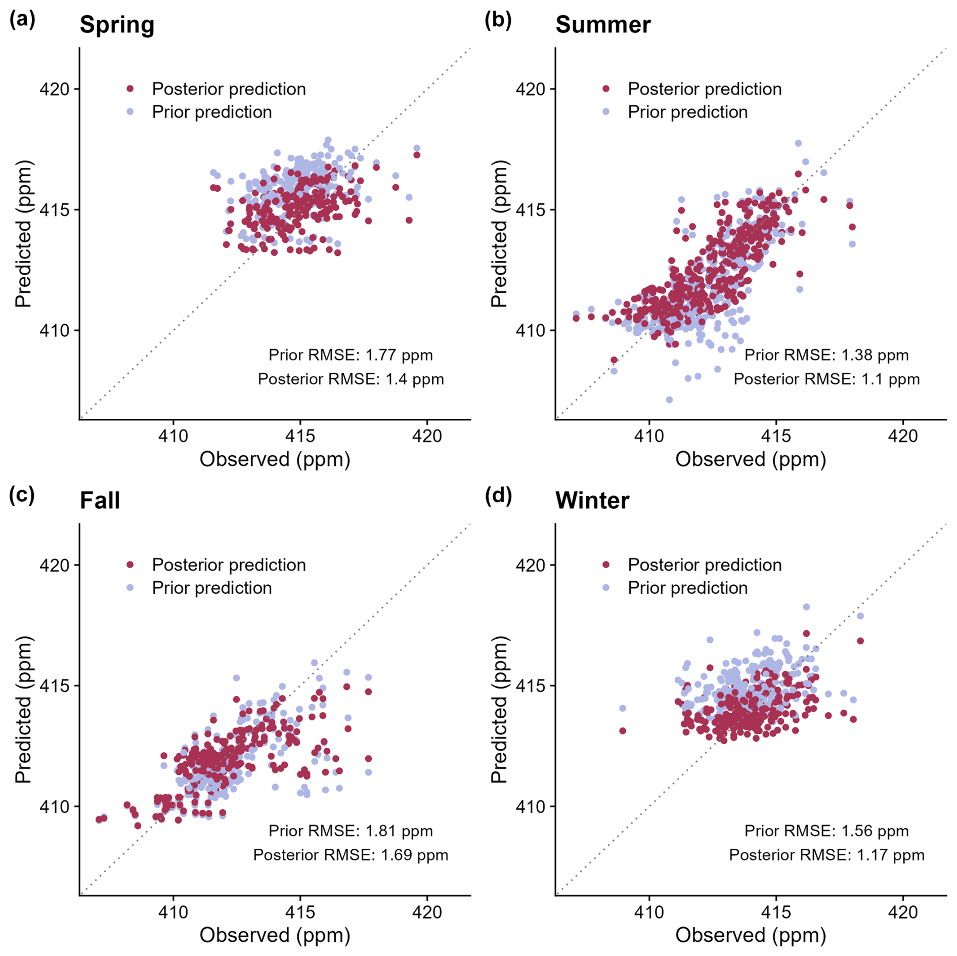
Figure 1 Comparison of seasonal GEOS-Chem XCO₂ predictions (ppm) using prior (blue) and posterior (purple) emissions and observed OCO-2 and OCO-3 concentrations (ppm). This result is based on the GP inversion model with a systematic bias of 0.5 ppm (Model 1). RMSE values for the prior and posterior model simulations are presented in the panel legends.

3.3 Inverse GP model evaluation

This section describes the evaluation of the GP inversion model using posterior predictive checks (PPCs). PPCs ensure that the inversion results accurately represent the observed data (Gelman et al., 1996). The method involves using the posterior distribution of the model parameters to generate new datasets, which are then compared to the actual observed data. PPCs assess whether the model is capable of producing data similar to the observed data, thereby providing insight into the model's ability to capture the data-generating process accurately. Section S1 describes the comparison of the different GP inversion model setups and how Model 1 performs the most accurately. Due to the best performance by Model 1, the rest of the results in this study are based on these outputs. Figure 2 shows PPCs using probability density functions (PDFs) for the middle of each season (except January) employing Model 1. Due to an insufficient number of OCO-2 and OCO-3 XCO₂ observations (N<10) in January, the PPC for February is included instead to represent the winter season. We construct the PDFs by utilizing local enhancements in XCO₂ concentrations after subtracting the OCO-2 or OCO-3 a priori XCO₂ and modeled BCs from the total satellite XCO₂ concentrations. The results in Fig. 2 demonstrate that the data generated from the Model 1 posterior parameters generally agree with observations.

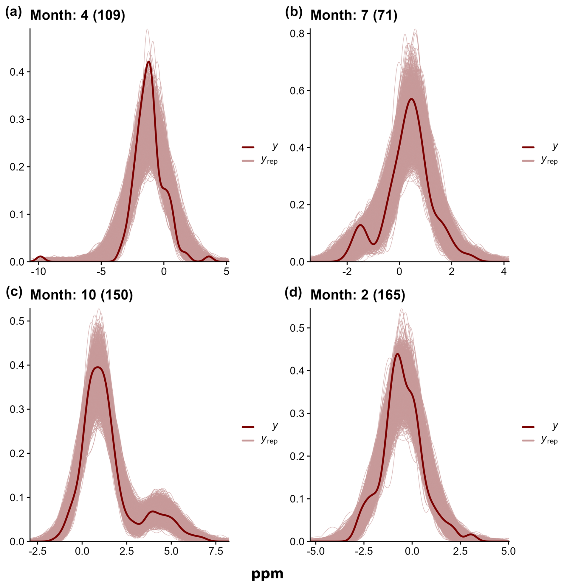
Figure 2 Evaluation of the GP inverse model (Model 1) performance using PPCs for months representative of each season in 2020 (April – spring; July – summer; October – fall; February – winter). The observed satellite XCO₂ data (y; in units of ppm) are represented by the bold lines, while the fine lines (y_rep) depict 4000 samples (in units of ppm) simulated with parameters drawn from the posterior distributions. Each sample (i.e., each fine line) for each month is of equivalent size to the number of the model–observation co-locations (noted in parentheses).

The comparison between the posterior predictions from the GP inversion and the observed satellite XCO₂ data indicates an improvement in the RMSE for all seasons (posterior RMSE values on average ∼ 17 % lower compared to prior model simulations), suggesting a more accurate model fit than the initial prior predictions (see Fig. 1). The GP inversion was also able to remove the majority of systematic bias imposed by the prior emissions and BCs used in the nested GEOS-Chem simulations and to improve the correlation with satellite XCO₂ observations. For spring months, posterior model simulations displayed a small bias of ∼ 0.3 ppm and a slightly improved correlation (R = 0.39) compared to prior model results. Posterior model results for the summer season displayed nearly zero bias and high correlation values of 0.79. The statistical evaluation of posterior model performance in the fall months improved compared to prior simulations with a bias of ∼ −0.1 ppm and a correlation of 0.57. Finally, for winter months, posterior results had a bias of ∼ 0.1 ppm, a significant improvement on the value of 1.0 ppm from the prior result, and a moderate correlation of 0.41. Overall, posterior results from the GP inversion performed in this study proved to be more accurate compared to prior simulations, suggesting that the emission estimates from these inverse model runs are robust, as expected from the PPCs.

3.4 Posterior emissions by season and sector

We estimate state-wide posterior emissions by season and sector based on Model 1, which was evaluated to perform the best according to the ELPD metric results (see Sect. S1), and the seasonally averaged posterior emissions are displayed in Fig. 3. Figure 4 shows the seasonal state-wide total posterior CO₂ fluxes from all three GP inversion models and the prior estimates for each source sector in California during 2020 (monthly averaged prior and posterior state-wide CO₂ fluxes displayed in Fig. S8). In general, all three GP inversion models are relatively consistent with respect to median posterior emission estimates for all source sectors and seasons. This consistency suggests that the GP models are robust with respect to inferring posterior emissions, despite slight performance variations by season and sector for each model. The rest of the results discussed in this section are focused on posterior estimates from Model 1. Figure 4 shows that posterior FF emissions align closely with the prior estimates on a seasonal scale, indicating consistency between the initial assumptions and the inversion-derived results. Posterior FF emissions are most consistent with prior estimates during the spring and summer months, when COVID-19 lockdown restrictions were most strict, suggesting that corrections applied to the 2020 Vulcan data using CARB data were reasonable compared to observations. For the fall and winter seasons, posterior FF emission estimates were reduced by 10–15 Tg CO₂ compared to a priori assumptions, although the reduction is within the margin of error. Seasonal posterior 2σ uncertainty (95 % confidence level) had a range of 20–30 Tg CO₂, which is on average ∼ 30 % of the seasonal posterior median FF emission values. Interestingly, from the monthly averaged state-wide emissions shown in Fig. S8, it can be seen that some months in the spring, summer, and fall of 2020 had posterior FF fluxes that were further reduced compared to the prior emissions, emphasizing the strong reduction in greenhouse gas (GHG) emissions due to COVID-19 lockdown restrictions.

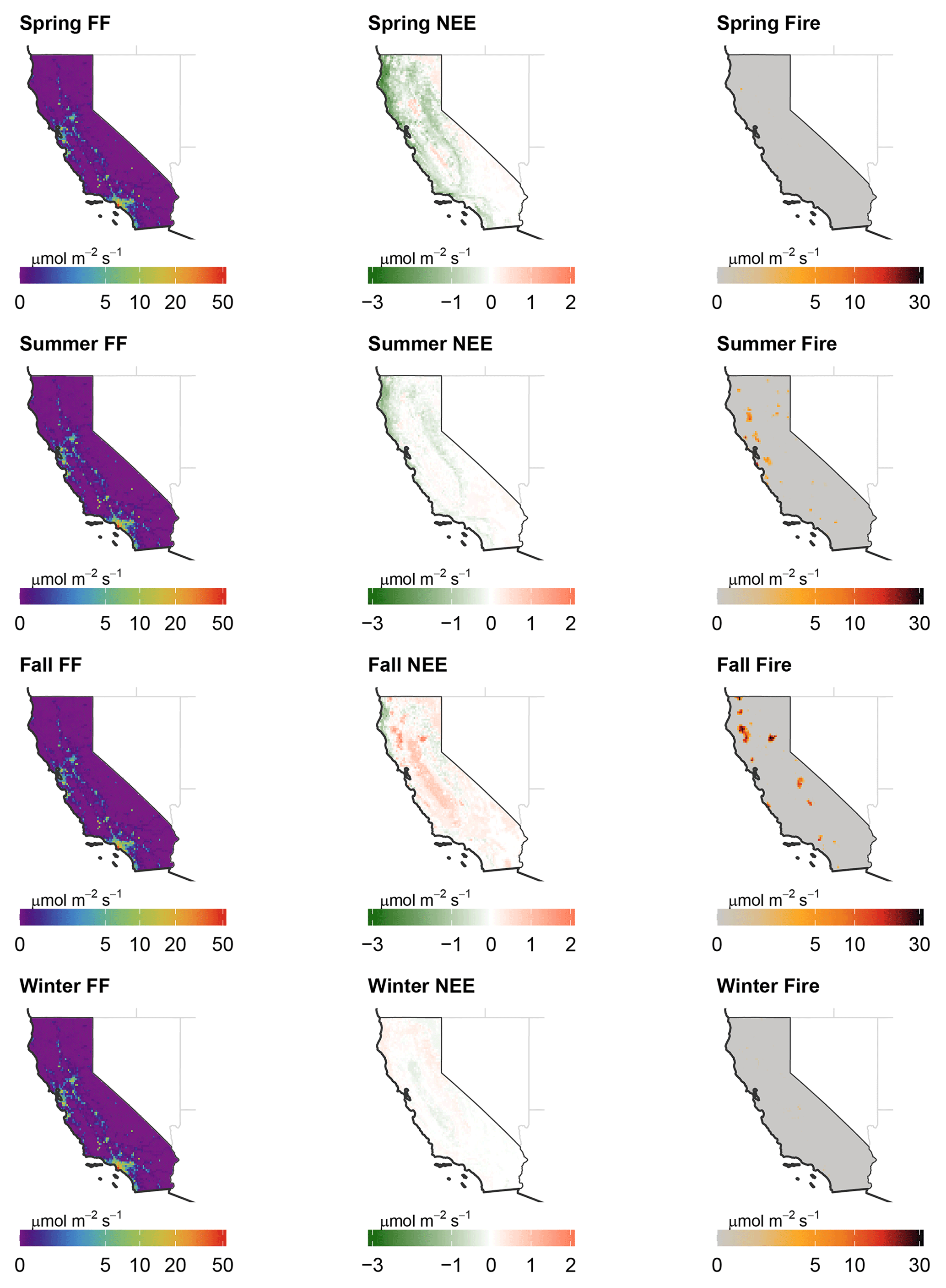
Figure 3 Seasonally averaged 2020 posterior CO₂ emissions (µmol m⁻² s⁻¹) for the state of California. Emissions from the terrestrial portion of California are shown for FF (left column), NEE (middle column), and Fire (right column) for the spring (first row), summer (second row), fall (third row), and winter (fourth row) months.

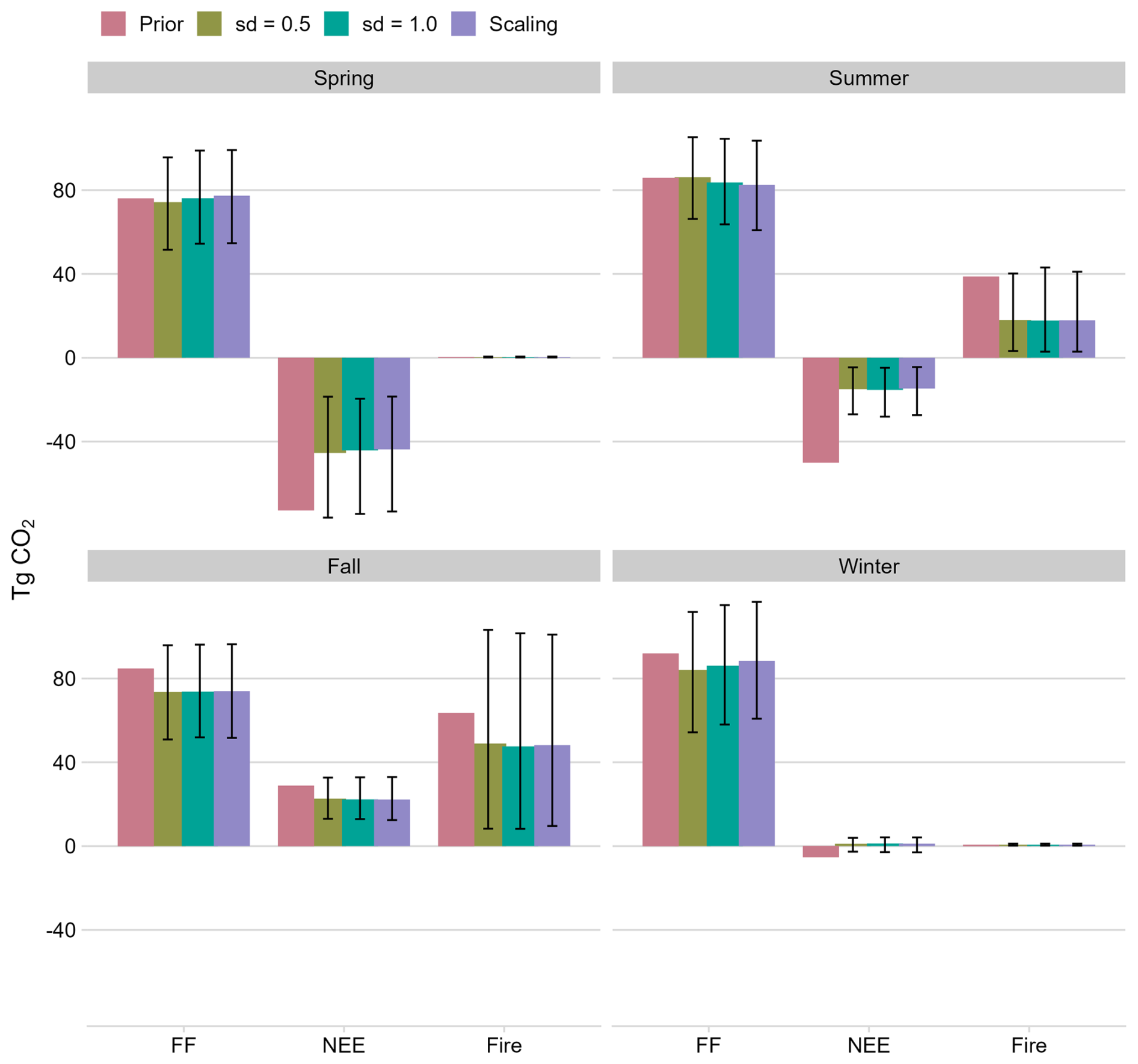
Figure 4 Sectoral emission estimates (Tg CO₂) by season from the scaled Vulcan a priori data and those using three distinct models: Model 1 (“SD = 0.5”), where a standard deviation (SD) of 0.5 ppm is applied to the prior probability distribution for the systematic bias; Model 2 (“SD = 1.0”), with a standard deviation of 1.0 ppm for the prior for the systematic bias; and Model 3 (“Scaling”), which optimizes the OCO-2 and OCO-3 a priori and model-predicted BC concentrations using scaling factors analogous to sector emission adjustments. The error bars in this figure reflect the 2σ uncertainty (i.e., 95 % confidence) values for each source sector. All 2σ confidence intervals were calculated using 4000 MCMC samples.

Posterior NEE fluxes from the GP inversion indicate that prior estimates assumed carbon uptake that was too strong during the drought year of 2020, suggesting an overestimation of the ecosystem's carbon sequestration capacity. Besides the fall season, posterior NEE was much less negative compared to the a priori fluxes, and it even transitioned from a small sink to a small source during the winter season (see Figs. 3 and 4). Posterior NEE fluxes are 25–35 Tg CO₂ less (lower NEE) compared to prior estimates in the growing seasons of the spring and summer. From Fig. S8, it can be seen that posterior NEE fluxes were near neutral during some of the summer months, compared to the large uptake suggested by prior fluxes. This is likely due to the strong drought and hot temperatures experienced in California during 2020 greatly reducing the CO₂ uptake during the growing season. The posterior adjustments during the fall were smaller and tended to be consistent with prior estimates from SMUrF. Posterior NEE emissions were consistent with the prior estimates within a 2σ uncertainty range for the spring and fall seasons; however, they were not statistically consistent for winter and summer months. Seasonal posterior NEE displayed the largest uncertainty values of all source sectors in California, and these uncertainties were on average ∼ 95 % of the seasonal posterior median emission value.

The inversion results for fire emissions imply that the prior estimates are consistent with the posterior results within the 2σ uncertainty range, although the posterior median values for summer were lower than the prior. As expected, prior and posterior CO₂ emissions from fires were small during the winter and spring months. Posterior median seasonal total CO₂ emissions ranged between 20 and 50 Tg CO₂ for the summer and fall seasons, respectively. Constraints from OCO-2 and OCO-3 observations reduced emission estimates compared to the prior during both of these seasons with the largest reduction occurring for summer months (−21 %). Seasonal posterior fire emissions displayed moderate to high uncertainty values, and these uncertainties were on average ∼ 80 % of the seasonal posterior median emission values.

3.5 State-wide posterior total CO₂ emissions

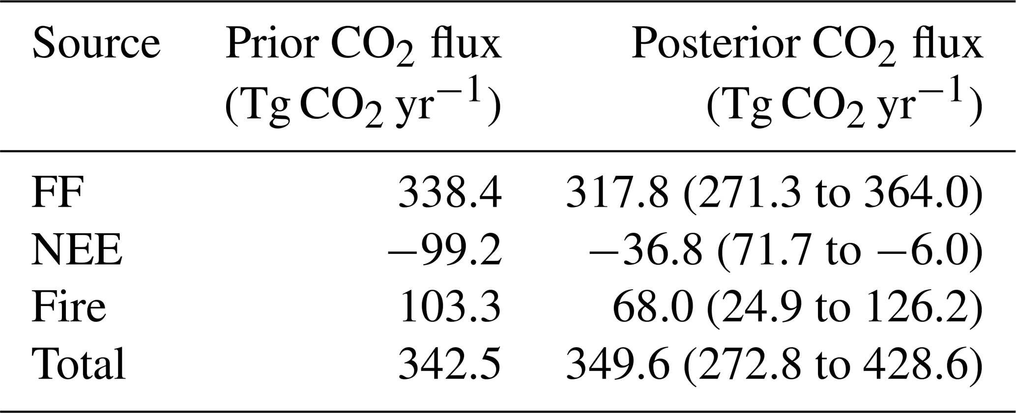
This section describes the annual state-wide CO₂ flux estimates constrained using OCO-2 and OCO-3 observations for each source sector in 2020. Table 2 shows the results of the prior and posterior state-wide flux estimates for each source sector and the overall net terrestrial flux. The PDFs of these annual state-wide CO₂ fluxes are displayed in Fig. 5 (seasonal sector CO₂ flux PDFs shown in Fig. S9). Both the table and figure show that the net state-wide CO₂ fluxes from both prior and posterior estimates are nearly identical at between 340 and 350 Tg CO₂ yr⁻¹. However, larger differences are evident when the state-wide annual emissions are broken down by source sector. Large constraints were imposed by OCO-2 and OCO-3 observations when focusing on NEE fluxes, where the posterior median estimate (−36.8 Tg CO₂ yr⁻¹; range of −71.7 to −6.0 Tg CO₂ yr⁻¹; 95 % confidence level) was 63 % lower (reduced carbon sink) compared to prior estimates (−99.2 Tg CO₂ yr⁻¹). Prior emissions from wildland fires were also reduced when constrained by satellite observations, as state-wide posterior estimates of 68.0 Tg CO₂ yr⁻¹ (range of 24.9–126.2 Tg CO₂ yr⁻¹; 95 % confidence level) were ∼ 35 % lower compared to a priori estimates. Finally, posterior FF emissions were 317.8 Tg CO₂ yr⁻¹ (range of 271.3–364.0 Tg CO₂ yr⁻¹; 95 % confidence level), which is ∼ 5 % lower compared to the prior estimates.

Table 2 The median prior and posterior (2σ range; 95 % confidence level) California CO₂ budget for 2020.

For total CO₂ fluxes, including all source sectors, California state-wide emissions are constrained with relatively high confidence using OCO-2 and OCO-3 XCO₂ observations, as the 2σ standard deviation on this total flux is ∼ 23 % of the annual median posterior estimate. Annual posterior emission estimates were most confident for FF sources, as the 2σ standard deviation from these sources was 47 Tg CO₂, which is ∼ 15 % of the posterior median value. Natural fluxes of CO₂ (i.e., NEE and wildland fire) in California displayed higher uncertainties with respect to their posterior estimates, as indicated by the wider PDFs in Fig. 5. The 2σ standard deviation of annual posterior NEE fluxes was on average ∼ 35 Tg CO₂, which is ∼ 95 % of the posterior median value, indicating that this is the most uncertain carbon flux when using satellites to constrain emissions. Posterior annual fire emissions were also associated with larger uncertainty, as the 2σ uncertainty range was 43 Tg CO₂ (64 % of the median posterior flux).

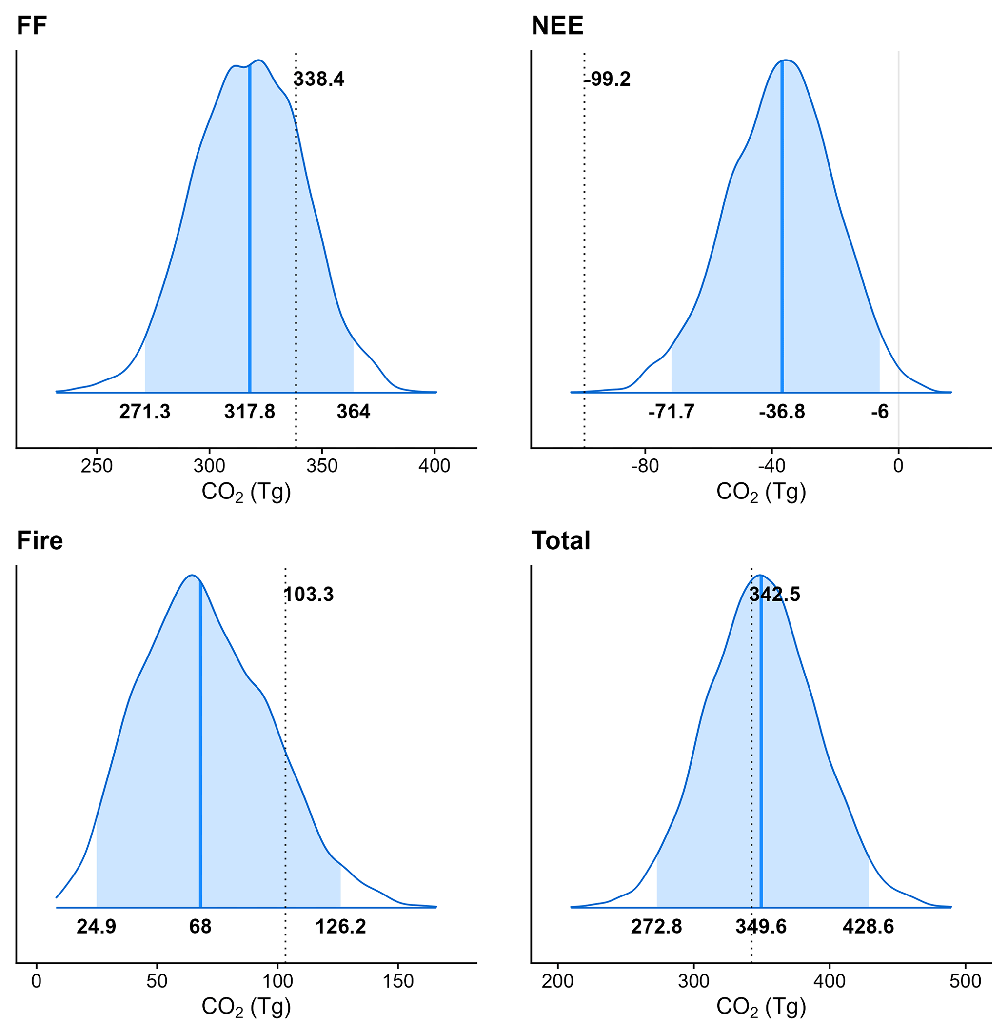
Figure 5 Annual CO₂ emission totals (Tg CO₂) for California by source sector in 2020. The numerical labels at the base of each PDF denote 2.5-, 50- (indicated by the bold vertical line), and 97.5-percentile estimates of the posterior emissions, respectively. The vertical dotted line indicates the prior emission estimate, with the corresponding value displayed. Note that the annual PDF presented here was derived by aggregating seasonal MCMC samples.

4 Discussion and conclusions

This study presents the first attempt to constrain state-wide CO₂ fluxes from California using spaceborne XCO₂ observations employing both OCO-2 and OCO-3. We chose to focus on the year 2020, as this time period was characterized by anomalous features likely impacting total CO₂ fluxes in California, including reduced anthropogenic emissions caused by the COVID-19 lockdown (Yañez et al., 2022), elevated wildfire activity (Jerret et al., 2022; Safford et al., 2022), and drought occurrence (Steel et al., 2022). In this study, assimilating OCO-2 and OCO-3 LN + LG XCO₂ observations into a GP inversion framework was demonstrated to be effective for constraining state-wide CO₂ fluxes with a high degree of accuracy. The median posterior top-down annual total CO₂ flux of 349.6 Tg CO₂ yr⁻¹ (range of 272.8–428.6 Tg CO₂ yr⁻¹; 95 % confidence level) was consistent with the a priori estimate and constrained with low 2σ uncertainty levels of ∼ 23 %. The posterior uncertainty estimates of this work are similar to other recent studies that have used OCO-2 and OCO-3 XCO₂ data to constrain city-wide CO₂ emissions in California (e.g., Roten et al., 2023), other city flux estimates (e.g., Wu et al., 2020), and country-wide CO₂ budgets (e.g., Byrne et al., 2023). Our study adds to the growing evidence on how satellite XCO₂ data can be used to confidently estimate city- to country-scale CO₂ fluxes.

CARB inventories for the years 2019 and 2020 suggest that anthropogenic FF CO₂ emissions were reduced by ∼ 10 % in 2020 compared to the year prior in California. In this study, the state-wide annual FF CO₂ source was estimated, using the GP inversion assimilating OCO-2 and OCO-3 XCO₂ data for 2020, to be 317.8 Tg CO₂ yr⁻¹, which is ∼ 5 % lower than the prior flux assumed. This top-down estimate is ∼ 15 % higher compared to the CARB 2020 inventory, which calculated state-wide anthropogenic CO₂ emissions for 2020 to be 277.7 Tg CO₂ yr⁻¹. The state-wide FF CO₂ emissions estimated using OCO-2 and OCO-3 data in this study had posterior uncertainties of ∼ 15 % on an annual scale and are, therefore, statistically consistent with the CARB 2020 inventory. The difference between the bottom-up and top-down median FF CO₂ emission estimate may be due to errors and uncertainties in the GP inversion and errors in the bottom-up CARB inventory, such as missing sources. It appears that the results in our study for FF emission estimates are robust, as they compare well to emission totals in California for the year 2020 from CARB and posterior top-down estimates are associated with low posterior uncertainty. Our PPC results, which compare the simulated data from posterior parameters with observations, provide additional confidence in our GP inversion models.

The main natural sources/sinks of CO₂ in California (i.e., NEE and wildland fire) were also estimated in this study using OCO-2 and OCO-3 XCO₂ data. The year 2020 was a year of drought in California and also resulted in extremely high levels of wildfire activity. The GP inversion resulted in posterior NEE fluxes that were greatly reduced compared to the initial best-guess a priori data. On an annual scale, the posterior estimate for NEE was −36.8 Tg CO₂ yr⁻¹, which was 63 % lower (reduced carbon sink) than prior estimates driven by satellite SIF retrievals. It is important to note that 2020 was towards the end of a multiyear drought that plagued California, and it would be expected that the terrestrial biosphere would be less effective in its uptake of carbon (Fu et al., 2022). It should also be noted that the median annual posterior NEE estimates derived in this study with satellite retrievals were associated with uncertainty levels of ∼ 95 %. The larger uncertainty value associated with our posterior NEE estimates, compared to FF sources, is expected, as satellite retrievals are less sensitive to small, diffuse signals of CO₂ enhancements associated with the terrestrial biosphere compared to larger FF point sources. Wildfire activity was elevated in California during the time of this study, and we estimated that these sources contributed 68.0 Tg CO₂ yr⁻¹ to the total state-wide annual carbon budget. The posterior estimate derived in our GP inversion was ∼ 35 % lower compared to the prior estimate; however, this estimate still represents highly elevated CO₂ emissions from this natural source. CARB estimated that ∼ 100 Tg CO₂ yr⁻¹ was emitted from wildfires in 2020 (https://ww2.arb.ca.gov/wildfire-emissions, last access: 22 December 2023), which is in line with the prior estimate from GFED4 used in our study. CARB uses an emissions model that is similar to GFED4, so this is to be expected. The lower posterior wildfire estimate using our GP inversion system was associated with uncertainty levels (∼ 64 % of the median posterior flux) that were lower compared to NEE and statistically consistent with the CARB 2020 state-wide estimate. Prior emission estimates from wildfires are generally uncertain, and satellite observations of the CO₂ resulting from these episodic events are challenging; thus, it is not surprising that posterior fire emissions are one of the more uncertain components of the 2020 California CO₂ budget.

Given that individual state- and country-wide CO₂ flux datasets generally have over a year of latency, satellite data become vital, as these spaceborne data are well equipped to provide more real-time estimates of these emissions. This is an important aspect of satellite data, especially during times of anomalous CO₂ fluxes due to economic activity, wildfire, or flood/drought. Both this study and the work by Roten et al. (2023) clearly demonstrated the ability of OCO-2 and, in particular, OCO-3 to help constrain FF emission estimates in California during the COVID-19 lockdown. OCO-3 is particularly effective for estimating city-wide (or other point- to area-source) fluxes using the data extracted from SAMs. These area-wide observations (∼ 80 km × 80 km) greatly improve the observational coverage compared to OCO-2 (narrow swath of only ∼ 10 km). These SAMs allow for observations that reduce errors in assumptions about mixing between the sources and observations and illustrate intra-city variability in XCO₂, which has been shown to allow for sector-based emission constraints in California (Roten et al., 2023). The recent launch of satellites and future plans for spaceborne instruments that retrieve greenhouse gas concentrations (e.g., GHGSat, CO₂M, Carbon Mapper, etc.) at high spatial resolution and precision, some of which will apply SAM observational approaches, should greatly improve the ability to accurately estimate CO₂ emissions at city to global scales. As demonstrated, our GP inverse model has the potential to utilize these new satellite datasets to estimate surface emissions in a near-real-time fashion, effectively incorporating the unique spatiotemporal coverage of space-based information.

In evaluating the GP inversion method used in this study compared to linear inverse classical Bayesian inversion (CBI) models (e.g., y = K λ+ϵ, commonly used in atmospheric inversions; Rodgers, 2000), advantages and disadvantages become apparent. The GP-based inversion method employed in this work offers several advantages over classical methods, as highlighted by Jeong et al. (2025). Jeong et al. (2025) presents the advantages of the GP method through inversion results from different approaches, and we briefly describe them here, focusing on the key points.

First, via simulations using multiple inverse modeling methods for constraining CO₂ fluxes in California when assimilating OCO-2 + OCO-3 XCO₂ observations, Jeong et al. (2025) demonstrated that the GP inversion yields superior results compared to the CBI method. Specifically, the CBI method failed to capture the FF scaling factor accurately at the 68 % confidence level. They repeated the inversion multiple times, and this result was consistent. Their work also showed that, without a proper prior distribution, a simple linear regression produced a physically implausible scaling factor for fire emissions. In our full Bayesian approach, we specify prior distributions for all parameters, including the scaling factors and kernel hyperparameters. Overall, the GP inversion offers substantial flexibility in modeling intricate, nonlinear dependencies without needing a prespecified model framework (Ebden, 2015).

Second, the CBI method typically relies on analytical solutions and lacks robust techniques for estimating crucial parameters, such as hyperparameters (e.g., variance of the diagonal elements) for the covariance matrix (i.e., the kernel). Consequently, many previous inversion studies have used prescribed values for hyperparameters. For instance, these studies often utilized known values from other work (e.g., Roten et al., 2023) or estimations derived from sensitivity analyses to construct the model–data mismatch covariance (Gerbig et al., 2003; Jeong et al., 2013; Johnson et al., 2016). Such approaches do not guarantee that the estimates are consistent with the observed data. In contrast, Jeong et al. (2025) showed that the GP method can infer the noise variance, with its median value closely aligning with the true value. This represents a significant advancement over previous approaches, as it enables the direct estimation of true noise variance from the input data. Moreover, the GP inversion intrinsically provides quantification of uncertainty, which proves advantageous in scenarios with limited data, such as in atmospheric inversions.

Third, the GP method includes the spatiotemporal kernel as its essential component, as shown in this work. While some previous work (e.g., Turner et al., 2020) used a covariance with both spatial and temporal components, many previous inversion studies have not used a fully spatiotemporal covariance. This is because it is not straightforward to estimate the hyperparameters for the spatiotemporal covariance in the CBI method based on analytical solutions (Jeong et al., 2025). For example, the work by Turner et al. (2020) did not estimate the covariance parameters in a way consistent with the data. Incorporating the spatiotemporal covariance as a core component of the inversion is a significant advantage of the GP method over the CBI method.

While the GP-based inversion has many advantages over CBI methods, the computational demands of the GP method increase significantly with larger datasets, potentially restricting its application in certain contexts (Williams and Rasmussen, 2006; Murphy, 2022), although recent development for high-performance computing (e.g., GPU-enabled tools) can alleviate this issue. Conversely, the linear inverse model, while less computationally demanding, assumes linearity and typically requires explicit assumptions about the underlying distribution, which may not always be valid and can lead to underestimation of model uncertainty (Wang, 2023). Overall, this study demonstrates the clear advantages of using GP-based inversion techniques, and this modeling framework should be considered for application in future studies for constraining GHG fluxes when assimilating satellite retrievals.