Satellite detection of NO₂ distributions using TROPOMI and TEMPO and comparison with ground-based concentration measurements

In this study we assess the capability of current-generation satellites to capture the variability of near-surface nitrogen dioxide (NO₂) monitoring data, with the goal of supporting health and regulatory applications. We consider NO₂ vertical column densities (VCDs) over the United States from two satellite instruments, the Tropospheric Monitoring Instrument (TROPOMI) and Tropospheric Emissions: Monitoring of Pollution (TEMPO), and compare them with ground-based concentrations as measured by the EPA's Air Quality System (AQS) monitors. While TROPOMI provides a longer-term record of assessment (2019–2023), TEMPO informs diurnal patterns relevant to evaluating peak NO₂. We analyze frequency distributions and quantify their similarity using the Jensen–Shannon divergence (JSD), where smaller values indicate better agreement. Satellite and ground monitor NO₂ distributions are most similar at non-roadway monitors (JSD =0.008) and are most different at interstate (JSD = 0.158) and highway (JSD =0.095) monitors. Seasonal analysis shows the greatest similarity in distributions in winter (JSD =0.010) and the greatest difference in summer (JSD =0.035). Across seasons and monitor locations, the calculated 13:30 LT TEMPO consistently exhibits JSDs that are better than or comparable to TROPOMI (TEMPO: 0.005–0.151; TROPOMI: 0.012–0.265). TEMPO's agreement with monitors, in both December 2023 and July 2024, is found to be best around midday, with non-road monitors in July having the best alignment (JSD =0.008) at 16:00 UTC (≈11:00 LT). These findings highlight the ability of TROPOMI and TEMPO to complement existing ground-based monitors and demonstrate their potential for monitor siting, regulatory, and public health applications.

1 Introduction

Nitrogen dioxide (NO₂) is a gas released through high-temperature combustion processes, such as the burning of fossil fuels (Lee et al., 1997; Richter et al., 2005), with on-road vehicles, power plants, and industrial processes representing the largest anthropogenic sources in the United States (US; van der A et al., 2008), as well as lightning NO_x emissions (Dang et al., 2023) and soil microbial activity (Huber et al., 2020) from natural sources. Exposure to elevated levels of NO₂ has been linked to respiratory and cardiovascular diseases (Mills et al., 2015; Urbanowicz et al., 2023; Meng et al., 2021), especially asthma in children (Mölter et al., 2014; Anenberg et al., 2022; Achakulwisut et al., 2019), as well as premature mortality (Camilleri et al., 2023; Hales et al., 2021; Huangfu and Atkinson, 2020) and other diseases (Xia et al., 2024; Bai et al., 2018). NO₂ plays a critical role in the formation of ozone, which also causes respiratory health problems and is harmful to ecosystems (Grulke and Heath, 2020; Sillman, 1999). It is also a precursor to nitrate (Behera and Sharma, 2012), a type of fine particulate matter (PM_2.5), which can penetrate deep into the lungs and exacerbate respiratory and heart conditions (Sangkham et al., 2024; Sharma et al., 2020), as well as causing premature death (Orellano et al., 2020; Thangavel et al., 2022).

Due to its radiative characteristics, NO₂ may be observed by satellites during daylight hours (Boersma et al., 2018; van Geffen et al., 2020; Veefkind et al., 2012) and NO₂ has emerged from satellite observations as one of the most air-quality-relevant pollutants (Holloway et al., 2021). Several studies have highlighted the potential for satellite NO₂ data to supplement ground-based networks to support health analysis and air quality management (Duncan et al., 2014; Lee and Koutrakis, 2014). The 2017 launch of the Tropospheric Monitoring Instrument (TROPOMI; Boersma et al., 2018; van Geffen et al., 2020; Veefkind et al., 2012) advanced these applications (Goldberg et al., 2021; Griffin et al., 2019; Kim et al., 2024; Yu and Li, 2022; Dressel et al., 2022; Goldberg et al., 2024; Lee et al., 2023). The Tropospheric Emissions: Monitoring of Pollution (TEMPO; Chance et al., 2019; Naeger et al., 2021; Zoogman et al., 2017) mission provides further advancements, with hourly daytime observations of NO₂ over North America and finer spatial coverage.

While advanced methods exist to calculate near-surface NO₂ from satellite columns (Ahmad et al., 2024; Kim et al., 2021; Shetty et al., 2024; Virta et al., 2023), there is also a strong interest in the utilization of satellite vertical column density (VCD) to directly infer NO₂ concentrations analogous to ground-based monitors (Kim et al., 2024; Lamsal et al., 2014; Griffin et al., 2019; Yu and Li, 2022; Zhang et al., 2018; Lamsal et al., 2015; Goldberg et al., 2021; Dressel et al., 2022; Goldberg et al., 2024; Harkey and Holloway, 2024; Bechle et al., 2013; Lee et al., 2023; Xu and Xiang, 2023). This study extends prior assessments of NO₂ column-to-surface agreement; we focus on frequency distributions to capture the net impact of day-to-day variability.

The relationship between surface NO₂ and column abundance is influenced by physical and chemical processes, many of which have seasonal components. In winter, shallow boundary layers trap pollutants near the surface, leading to higher surface concentrations and increasing surface-to-column agreement (Harkey et al., 2015). In summer, higher temperatures and increased sunlight accelerate photochemical reactions, converting NO₂ into ozone and other secondary pollutants and decreasing surface-to-column agreement (Boersma et al., 2009). Seasonal changes in emissions, such as high building-heating emissions in winter and high power-plant emissions in summer (Frost et al., 2006; Levinson and Akbari, 2010), interact with atmospheric processes, causing an increase in NO₂ column abundance in winter in four-season climates (Shah et al., 2020). Processes affecting the sources and sinks of NO₂ at the surface and through the vertical column can also lead to temporal lags, with peak surface NO₂ preceding peak column NO₂ in the mornings (Harkey and Holloway, 2024).

Frequency distributions capture the variability, extremes, and patterns of pollutant abundance, relevant to air quality standards, pollution trends, and the effectiveness of emission control measures (Knox and Lange, 1974; Pollack, 1975; Venkatram, 1979; Chowdhury et al., 2021; Mondal et al., 2022). For example, Mondal et al. (2022) used frequency distributions of ground-based monitors to examine changes in air quality across Delhi and Kolkata during COVID-19 lockdown phases, showing how reduced human activity led to shifts in pollutant levels. We extend this line of analysis by comparing NO₂ distributions across multiple dimensions with TROPOMI and include time-of-day- and resolution-dependence of results using data from TEMPO.

In this work, we consider the following questions: (1) How do the distributions of satellite NO₂ VCD measurements compare with those for near-surface NO₂? (2) To what degree do new hourly data from TEMPO improve the agreement between surface- and space-based NO₂ distribution measurements? For both questions, we consider spatial variability, especially proximity to roadways, and temporal variability, including seasonality and diurnal variability. By considering the ability of satellites to capture peak NO₂ values in a comparable distribution to surface data, we consider how satellite measurements of VCD can support air quality management, improve health impact analysis, and inform air pollution monitor siting.

2 Data and methods

In this study, we evaluate the ability of two satellite instruments, TROPOMI and TEMPO, to capture the spatial and temporal variability in NO₂ surface concentration distributions across the continental United States (CONUS), as measured by AQS monitors. By comparing the coefficient of variation (CV) and Jensen–Shannon divergence (JSD) between satellite and monitor data, we aim to assess the alignment between the datasets.

2.1 EPA surface monitor data

The Environmental Protection Agency (EPA) Air Quality System (AQS) contains hourly NO₂ measurements from ground-based monitors, providing high temporal resolution data that are critical for assessing compliance with the US National Ambient Air Quality Standards (NAAQS). There are two NAAQS related to NO₂: one for annual average concentration, set at 53 ppb, and one based on peak 1 h concentrations, set at 100 ppb, based on the 3 year average of the 98th percentile of the yearly distribution of daily maximum 1 h NO₂ concentrations (EPA, 2010). Enforcement of these standards relies on data from AQS NO₂ monitors, a network that included 431 monitors as of August 2024. Because NO₂ has a relatively short atmospheric lifetime, typically ranging from a few hours to a day, depending on meteorological conditions (Lange et al., 2022; Liu et al., 2021), ground monitors are expected to capture local conditions (Wang et al., 2020).

The EPA AQS dataset (EPA, 2025) was used to access NO₂ monitor data for the years 2019 through 2023 from all available sites in CONUS during this time period (503 unique monitors from 2019 to 2023). We note that there are some areas that are overrepresented by NO₂ monitors and others that are lacking monitors. Specifically, most monitors are located in urban areas, especially on the East Coast and in southern California, meaning that rural areas tend to be less represented by ground monitors (Kerr et al., 2023). Most monitors use a chemiluminescence method, where the amount of NO₂ that is converted to NO is measured by a molybdenum oxide converter (Fontijn et al., 1970). The converter also reacts with other oxidized nitrogen compounds, such as nitric acid (HNO₃) and peroxyacetyl nitrate (PAN), to form NO (Dunlea et al., 2007; Steinbacher et al., 2007); this can lead to an overestimation of NO₂. Corrections for this bias have been applied when comparing with satellite observations (e.g., Cooper et al., 2020; Lamsal et al., 2015; Li et al., 2021). Uncorrected AQS NO₂ measurements have been used for determining compliance with the NAAQS and for health assessments; this is the approach we take here, consistent with prior studies focused on regulatory relevance (Novotny et al., 2011; Penn and Holloway, 2020; Harkey and Holloway, 2024; Goldberg et al., 2021; Kim et al., 2024; Duncan et al., 2013; Qin et al., 2019). More recently, some NO₂ monitors have been added to the network that measure “true NO₂” using cavity attenuated phase shift spectroscopy (CAPS, Kebabian et al., 2005). These monitors are expected to be more representative of ground-level NO₂ concentrations and should have less overestimation, since they directly measure NO₂ and no other species (Ge et al., 2013). Some of the monitors used in this study use CAPS methodology to measure NO₂. We discuss the comparison of CAPS with traditional NO₂ monitors in Sect. 3.1.

Hourly AQS measurements at 13:00 and 14:00 local time (LT) were averaged to align with the TROPOMI overpass of ≈13:30 LST. Hourly AQS measurements from 12:00 to 23:00 GMT were compared with hourly TEMPO data for daylight hours. For both the TROPOMI and TEMPO analyses, AQS data were filtered to ensure consistency with satellite data availability. As a result of filtering monitoring data for TROPOMI and TEMPO separately, the subsets of monitor data available for comparison with each instrument differ, even for the same time periods.

2.2 TROPOMI data

The Tropospheric Monitoring Instrument (TROPOMI; Copernicus Sentinel-5P, 2018) is on board the Copernicus Sentinel-5 Precursor satellite, which has a daily local overpass time of ≈13:30 LST (Veefkind et al., 2012). Currently, the highest resolution of TROPOMI is 3.5 km×5.5 km at nadir, having increased from 3.5 km×7.0 km since 6 August 2019. Daily TROPOMI NO₂ data for the years 2019 through 2023 were allocated to a 4 km×4 km grid over CONUS using the Wisconsin Horizontal Interpolation Program for Satellites (WHIPS; Center for Sustainability and the Global Environment, 2024; Harkey et al., 2015, 2021; Harkey and Holloway, 2024; Penn and Holloway, 2020). Using WHIPS, we also remove data with a quality flag lower than 0.75. Each monitor location was compared with the 4 km×4 km gridded TROPOMI value in the corresponding grid cell. December 2023 and July 2024 4 km×4 km TROPOMI NO₂ data were also collected for each of the monitors for comparison with TEMPO data.

A 4 km×4 km oversampled grid is used as opposed to the 1 km×1 km oversampled grid since this study focuses on daily observations and the 1 km×1 km grid is best suited for monthly or annual averages (Goldberg et al., 2021). To ensure that a valid number of TROPOMI pixels were being represented despite the coarser grid resolution, we analyzed the number of ground monitors falling within each TROPOMI pixel by performing a spatial join between ground monitor locations and the oversampled 4 km×4 km TROPOMI grid. About 97 % of TROPOMI pixels contain only one monitor, with only a small number of pixels (2.7 %) containing more than one. Figure S1 in the Supplement shows the number of monitors per TROPOMI pixel (locations where there are more than one monitor per TROPOMI pixel) and the number of valid TROPOMI retrievals from 2019 to 2023 at each grid cell, confirming that monitors are well-distributed enough to not disproportionately cluster within a small subset of satellite pixels. Since monitors are spread across the entire US and most are at least 4 km apart, there is generally sufficient separation to ensure that most monitors are assigned to distinct TROPOMI pixels rather than falling into the same grid cells repeatedly.

2.3 TEMPO data

The TEMPO instrument launched onboard the Intelsat 40e mission (NASA Langley Research Center, 2024), a geostationary satellite, on 7 April 2023. TEMPO provides hourly measurements of atmospheric pollutants over North America (Chance et al., 2019; Naeger et al., 2021; Zoogman et al., 2017). TEMPO achieves a spatial resolution of approximately 2.1 km in the north–south direction and 4.5 km in the east–west direction at the center of its field of regard (FOR), centered around 36.5° N and 100° W (Chance et al., 2019). The TEMPO Level-3 (L3) NO₂ data (Suleiman, 2024) used in this study were accessed through NASA's EarthData Search portal.

In order to synchronize TEMPO and ground-based hourly measurements, TEMPO timestamps were rounded to the nearest hour, with mid-hour values rounded up. All files within each rounded-hour group were averaged, producing a single NO₂ value per hour per day. Only TEMPO observations with a main data quality flag of 0 and cloud fraction at or less than 0.2 were retained, in line with TEMPO documentation guidelines (NASA Langley Research Center, 2024).

For the comparison with TROPOMI, the UTC equivalents of 13:00 and 14:00 LT were determined for each time zone, based on the latitude and longitude of each monitor location. TEMPO NO₂ values corresponding to these calculated UTC hours were averaged to align with the TROPOMI overpass time (≈13:30 LST). Similarly, for ground-based measurements, the monitor data were filtered to include only values corresponding to 13:00 and 14:00 LT and then averaged.

2.4 Monitor classification

To classify the monitors by roadway proximity, the state-level Census Bureau's 2021 TIGER/Line Shapefiles for Primary and Secondary Roads (U.S. Census Bureau, 2025a) were combined to form a comprehensive dataset for the CONUS domain.

To evaluate how TROPOMI and ground-based monitor NO₂ values vary by proximity to a road, monitors were also assigned to different groups based on their distance from a road (≤20 m, 20–50 m, 50–300 m, 300 m–1 km, and >1 km), with buffer distances calculated from the road shapefiles (Fig. S3). There were nine monitors that were 20 m or less away from a road, 66 between 20 and 50 m from a road, 108 between 50 and 300 m, 167 between 300 m and 1 km, and 153 that were greater than 1 km from a road.

Roads were also classified into three categories: (1) interstates, (2) highways, and (3) other roads, based on their route type code (RTTYP) values. Where monitors are considered as representing a roadway category, we followed the criteria of the EPA Near-Road Network (Gantt et al., 2021; Kim et al., 2024) to merge monitor locations with road buffers, considering the 50 m buffer recommended by the EPA, as well as a less restrictive 300 m buffer. In each case, monitors inside the buffer of a particular roadway type were classified as representing that category. If a monitor fell within multiple buffers, it was assigned the classification of the largest road type. Monitors not falling within any buffers were classified as “non-roadway.”

Using the 50 m buffer, 58 monitors were classified as “interstate,” 17 as “highway,” and 428 as “non-roadway” (Fig. S2; no monitors classified as “other roads”). Using the 300 m buffer, 91 monitors were classified as “interstate,” 90 as “highway,” 320 as “non-roadway,” and 2 as “other roads.” Since there were no monitors classified as “other roads” for the 50 m buffer, this category is excluded from the analysis.

We classified interstate monitors as urban or rural using the US Census Bureau 2020 Urban Areas TIGER/Line Shapefiles (U.S. Census Bureau, 2025b). Only one interstate monitor was identified as rural, so this analysis is not included.

2.5 Data analysis

The coefficient of variation (CV) was calculated for ground-level monitor data and for satellite data. This metric was used to compare the relative variability of NO₂ distributions between satellite and ground-level data despite different measurement units (Aerts et al., 2015). The CV is defined as the ratio of the standard deviation (σ) to the mean (μ) of the data:

$$\mathrm{CV}=\left({\displaystyle \frac{\mathit{\sigma }}{\mathit{\mu }}}\right)\times \mathrm{100}.$$

The Jensen–Shannon divergence (JSD) is used to quantify the similarity between the distributions of NO₂ from the satellite and ground-level monitors despite the different measurement units (Menéndez et al., 1997). The JSD is a robust metric for comparing probability distributions that is used within a wide variety of fields, including machine learning (Thiagarajan and Ghosh, 2024; Saurette et al., 2023; Tsigalou et al., 2021; Melville et al., 2005), data science (Toledo et al., 2022; Zhao et al., 2024), biology (Yan et al., 2021; Jones et al., 2023; Ahmed et al., 2023), and meteorology (Kibirige et al., 2023). In environmental research using satellite data, the JSD has shown that the Mangrove Forest Index (MFI) from Sentinel-2 imagery outperforms traditional vegetation indices in distinguishing submerged mangrove forests (Jia et al., 2019). In air quality, the JSD has been used to compare an air quality index (AQI) with measurements of specific air pollutants (Wang and Zhang, 2022).

To calculate the JSD, each dataset was binned, with a bin size of 1 ppb (for ground monitors) or 1×10¹⁵ molec. cm⁻² (for satellite data), for the range from 0 to 40 ppb or 40×10¹⁵ molec. cm⁻², with an additional bin for values exceeding 40 ppb or 40×10¹⁵ molec. cm⁻². For visualization purposes, the frequency distributions are binned for data from the ground monitors ranging from 0 to 40 ppb and for satellite data ranging from 0 to 30×10¹⁵ molec. cm⁻², with additional bins for values exceeding 40 ppb or 30×10¹⁵ molec. cm⁻². Depending on the specific analysis, NO₂ data are grouped by

• distance from roadways (in m): TROPOMI daily data from 2019 to 2023 (and corresponding ground monitor data) are grouped by proximity to roads to assess spatial alignment;

• season: TROPOMI daily data from 2019 to 2023 (and corresponding ground monitor data) are grouped by season to analyze temporal alignment;

• month: TROPOMI daily data from December 2023 and July 2024, along with TEMPO and ground monitor data at the TROPOMI overpass time (≈13:30 LT, represented by the average of 13:00 and 14:00 LT data), are grouped by month to compare the temporal differences in alignment between TEMPO and TROPOMI; and

• road type (interstate, highway, non-roadway): TROPOMI (daily), TEMPO (calculated overpass time and hourly), and ground monitor data are grouped by road type to evaluate varying alignment based on road classification.

Binned data were then normalized to form probability distributions. The divergence was calculated as

$$\mathrm{JSD}\left(P,Q\right)={\displaystyle \frac{\mathrm{1}}{\mathrm{2}}}\left[D_{\mathrm{KL}}\left(P\right|\left|M\right)+D_{\mathrm{KL}}\left(Q\right|\left|M\right)\right],$$

where P and Q represent the probability distributions from the monitor and satellite data, respectively, and M is the average of P and Q. The divergence D_KL is the Kullback–Leibler divergence between each distribution and its mean (Clim et al., 2018). JSD values range from 0 to 1, with lower values indicating greater similarity between the satellite and monitor distributions. In general, JSD<0.1 indicates very good alignment, $\mathrm{0.1}\le \mathrm{JSD}<\mathrm{0.3}$ indicates moderate alignment, and JSD≥0.3 (Kibirige et al., 2023) indicates poor alignment.

3 Results

To evaluate the agreement between satellite-measured and monitored NO₂ distributions, we consider the impact of monitor location using TROPOMI, the impact of season using TROPOMI, the comparison of distributions between TROPOMI and TEMPO, and the impact of time of day using TEMPO.

3.1 Alignment of TROPOMI NO₂ distributions with surface NO₂ distributions

This section analyzes TROPOMI and ground-based NO₂ measurements across varying distances from roads and different seasons, as well as at monitors located near interstates, highways, and non-roadway sites. Our results show that, as the distance from roads increases, the distributions of surface and column NO₂ become more similar. Monitor distributions near interstates and highways exhibit lower agreement with TROPOMI distributions, compared with those farther from major roadways. Seasonally, alignment is strongest in winter and weakest in summer.

Figure 1 illustrates the distribution of NO₂ levels measured by AQS ground-based monitors and TROPOMI observations as a function of distance from roadways using daily measurements from 2019 to 2023. For both data sources, mean, peak, and minimum NO₂ are all highest in the 20–50 m distance category (the second closest near-road category). NO₂ abundance decreases as the distance to the road increases and, to a lesser extent, as the distance to the road decreases. The somewhat lower abundance in the ≤20 m category vs. the 20–50 m category may be due to the speciation of NO_x, where nitric oxide (NO) is more abundant and converts to a higher fraction of NO₂ as the distance to the road increases (Kimbrough et al., 2017). Most direct vehicle emissions are in the form of NO and, close to the roadway, NO and NO₂ readily convert between these forms. Limited ozone availability – especially during stable conditions, which contribute to suppressed vertical mixing – can slow the conversion of NO to NO₂ (Richmond-Bryant et al., 2017). As a result, NO₂ may initially be suppressed very close to the road, and changes in total NO_x are primarily driven by mixing and dilution rather than chemical transformation. NO₂ probably peaks in the 20–50 m range because this zone allows for sufficient time and space for NO to oxidize to NO₂ while still being close enough to the emission source to experience elevated concentrations; beyond this range, concentrations decrease with distance due to dispersion and dilution of pollutants into the surrounding atmosphere. Mean monitored NO₂ is 6.85 ppb at ≤20 m, 10.47 ppb at 20–50 m, 4.53 ppb at 50–300 m, 3.71 ppb at 300 m–1 km, and 2.80 ppb at >1 km. Mean TROPOMI NO₂ is 3.38×10¹⁵ molec. cm⁻² at ≤20 m, 4.21×10¹⁵ molec. cm⁻² at 20–50 m, 3.00×10¹⁵ molec. cm⁻² at 50–300 m, 3.72×10¹⁵ molec. cm⁻² at 300 m–1 km, and 3.13×10¹⁵ molec. cm⁻² at >1 km. Monitor values show a higher sensitivity to roadway proximity, where the highest mean monitored concentration is 375 % of the lowest mean concentration, compared with TROPOMI, where the highest mean VCD is 140 % of the lowest mean VCD.

Monitored NO₂ levels drop over 50 % at ≈50 m from the roadway (based on change in the mean, upper 2.5 interquartile range (IQR), and upper 1.5 IQR), a finding that compares with a 31 % reduction in NO₂ between 20 and 300 m from Kimbrough et al. (2017), as well as other studies that identify a decrease in NO₂ at further distances (Karner et al., 2010; Richmond-Bryant et al., 2017). TROPOMI VCDs also show the greatest change with roadway distance at ≈50 km, but by less than 30 % (based on change in the mean, upper 2.5 IQR, and upper 1.5 IQR).

Just as total NO₂ abundance, from both monitor and satellite data, is highest at distances of 20–50 m from the roadway, the range of daily values is also widest for the 20–50 m range and smallest at the >1 km range. Monitored values have a standard deviation of 8.24 ppb in the 20–50 m range and a standard deviation of 3.39 ppb in the >1 km range. The distribution of satellite data does not vary as much in size across roadway locations, with a standard deviation of 3.90×10¹⁵ molec. cm⁻² for the 20–50 m range and 3.31×10¹⁵ molec. cm⁻² for the >1 km range. In the 20–50 m range, the upper IQR of AQS NO₂ is 38 % higher than the mean. TROPOMI shows less variability than the monitors, with the 20–50 m upper IQR 16 % higher than the mean. As distance from the roadway increases, the distributions of data from the ground and satellite become more comparable. In the >1 km range, the upper IQR of monitor NO₂ is 23 % higher than the mean and the upper IQR of satellite data is 15 % higher than the mean. The ranges show more similarity at greater distances from the roadway but, even at distances of >1 km, the range of monitored values exceeds the range of satellite VCDs. These patterns agree with Kim et al. (2024), who found that surface monitors show better agreement with TROPOMI farther from major roads. This improved alignment at greater distances probably reflects the reduced influence of localized emission sources, which tend to create sharp gradients and rapid variability near roads. In areas farther from traffic, NO₂ concentrations vary more gradually or are generally more uniform. As a result, surface monitors away from roads reflect broader conditions, in better agreement with the coarser spatial resolution of TROPOMI.

When analyzed by season (Fig. S4), the relationships are similar, except winter shows the highest IQRs, with the 20–50 m distance group having an IQR of 11.40 ppb for monitors and 4.96×10¹⁵ molec. cm⁻² for TROPOMI, and summer shows the lowest IQRs for both monitors (IQR =9.05 ppb) and TROPOMI (IQR $=\mathrm{1.71}\times {\mathrm{10}}^{\mathrm{15}}$ molec. cm⁻²). In the >1 km distance group, again winter has the highest IQRs (monitor IQR =4.60 ppb; TROPOMI IQR $=\mathrm{3.95}\times {\mathrm{10}}^{\mathrm{15}}$ molec. cm⁻²) and summer the lowest IQRs (monitor IQR =2.05 ppb; TROPOMI IQR $=\mathrm{1.55}\times {\mathrm{10}}^{\mathrm{15}}$ molec. cm⁻²).

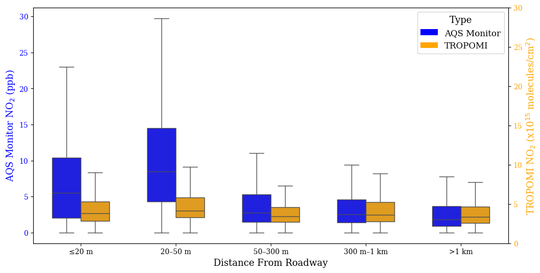
Figure 1 Box plots showing median and interquartile ranges of all daily 2019 to 2023 NO₂, as measured by AQS monitors (blue) and TROPOMI (orange) across various distances from roadways, with the whiskers extending to the 1.5 IQR range. No outliers are shown. The left y axis represents AQS monitor values in parts per billion (ppb) and the right y axis represents TROPOMI NO₂ values in 10¹⁵ molec. cm⁻². The distance categories from the roadway are ≤20 m, 20–50 m, 50–300 m, 300 m–1 km, and >1 km.

To consider the shape of monitor and satellite NO₂ distributions, we consider the effect of season in Fig. 2. The winter distributions (Fig. 2a, calculated from December, January, and February data) exhibit the longest tails and highest NO₂ values. In winter, the 90th percentile of monitoring data is 14.80 ppb and the 90th percentile of TROPOMI data is 10.93×10¹⁵ molec. cm⁻². Spring distributions (Fig. 2b; March, April, and May) show intermediate behavior, with lower values and shorter tails than winter and fall but higher values than summer (90th percentile from monitors =9.71 ppb; 90th percentile from TROPOMI $=\mathrm{6.19}\times {\mathrm{10}}^{\mathrm{15}}$ molec. cm⁻²). In summer (Fig. 2c, June, July, and August), the distributions exhibit the shortest tails and the lowest NO₂ values (90th percentile from monitors =9.00 ppb; 90th percentile from TROPOMI $=\mathrm{4.57}\times {\mathrm{10}}^{\mathrm{15}}$ molec. cm⁻²). Fall (Fig. 2d; September, October, and November) also shows intermediate behavior, generally between winter and spring (90th percentile from monitors =12.15 ppb; 90th percentile from TROPOMI $=\mathrm{7.44}\times {\mathrm{10}}^{\mathrm{15}}$ molec. cm⁻²). The higher NO₂ values in winter from monitor and TROPOMI data are attributed to reduced photochemical activity in winter leading to longer NO₂ lifetimes (Harkey et al., 2015; Boersma et al., 2009; Shah et al., 2020).

The highest percentage frequencies for the monitor and TROPOMI distributions generally occur within the 1–2 ppb or 1–2×10¹⁵ molec. cm⁻² bin. However, the winter TROPOMI distribution peaks in the 2–3×10¹⁵ molec. cm⁻² bin, with a percentage frequency of 18.14 %, compared with the winter monitor distribution, with a highest frequency of 14.33 %. The highest percentage frequency in spring from TROPOMI is 30.39 % versus that from the monitor, 24.15 %; in summer that from TROPOMI is 34.35 % versus that from the monitor, 24.68 %; in fall that from TROPOMI is 24.90 % versus that from the monitor, 18.89 %. These results indicate that TROPOMI consistently records higher peak frequencies than the monitors, whereas monitors consistently show a wider distribution.

Figure 2 provides a seasonal breakdown of the coefficient of variation (CV) and Jensen–Shannon divergence (JSD) for both monitor and TROPOMI data across all monitors. Summer exhibits the highest variability in monitored NO₂ concentrations (CV=127.99 %) but the lowest variability in satellite observations (CV=78.00 %). The highest variability in TROPOMI occurs in winter (CV=103.51 %), similar to the variability from monitor data (CV=104.48 %). Satellite CVs generally follow a similar pattern to that of monitors, though the overall variability is lower for satellite data across seasons.

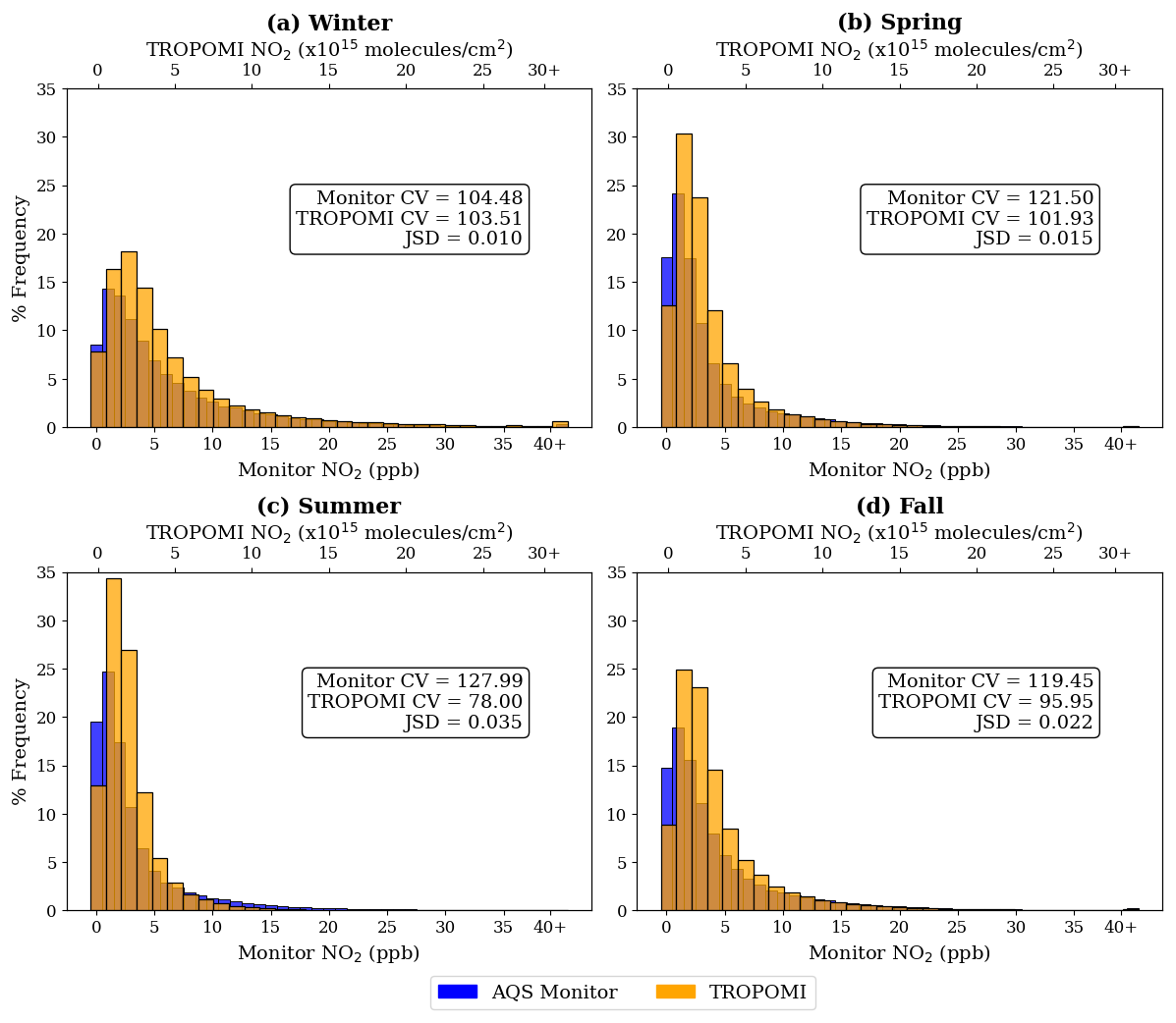
Figure 2 Seasonal frequency distributions of 2019–2023 NO₂, as measured by AQS ground-based monitors (blue) and TROPOMI (light orange) data for four seasons: (a) winter, (b) spring, (c) summer, and (d) fall. The x axes indicate the range of NO₂, with the primary lower x axis showing monitor NO₂ concentrations in parts per billion (ppb) and the secondary upper x axis showing TROPOMI NO₂ VCD in 10¹⁵ molec. cm⁻². The boxes show the coefficient of variation (CV; %) and Jensen–Shannon divergence (JSD) for each season.

This reduced variability in satellite observations can probably be attributed to the vertical mixing reflected in satellite retrievals, as well as horizontal spatial averaging reflected in satellite data, versus point-based NO₂ that are captured by ground monitors. This finding is consistent with previous studies that highlight the spatial averaging nature of satellite-based measurements, which integrate NO₂ amounts over a larger area than the point-based monitors (Ialongo et al., 2020).

Across all seasons shown in Fig. 2, JSD values are all low (<0.1), indicating that TROPOMI may be good at predicting surface NO₂ across seasons. The alignment is strongest in winter (JSD=0.010), while the divergence is highest in summer (JSD=0.035), meaning that the monitors and TROPOMI align best when the NO₂ lifetime is long in the colder months and they align worst when the NO₂ lifetime is short in the warmer months. The better alignment in winter could also be attributed to winter having the largest range of values in the data, which reduces the sensitivity of the JSD calculation to small differences in the distributions. A wider spread in NO₂ values means that relative discrepancies between TROPOMI and monitor measurements are smaller in proportion to the total variability, potentially leading to greater similarity.

Across seasons, we find that CAPS or “true NO₂” monitors tend to have slightly worse alignment with TROPOMI than traditional chemiluminescence monitors. Out of the monitors used in this study, 102 were identified as CAPS monitors and 401 as traditional monitors. In winter, CAPS monitors have a JSD of 0.027 and traditional monitors a JSD of 0.009. In summer, CAPS monitors have a JSD of 0.078 and traditional monitors a JSD of 0.03. With all seasons combined, CAPS monitors have a JSD of 0.047 and traditional monitors have a JSD of 0.016.

Table 1 shows the CV and JSD for both monitor and satellite data from 2019 through 2023, aggregated across all seasons and separated by monitor classification (interstate, highway, and non-roadway), where roadway monitors are classified as being within 50 m (Table 1a) or 300 m (Table 1b) of a road. For the 50 m buffer (Table 1a), the coefficient of variation for ground-based monitor data increases progressively from interstate monitor locations to non-roadway locations, with interstate monitors exhibiting the lowest variability (CV=75.07 %) and non-roadway monitors showing the highest variability (CV=118.17 %). This indicates that NO₂ concentrations measured by ground monitors in interstate areas are more consistent, compared with non-roadway regions. This pattern is mirrored in the satellite data, with CV values ranging from 91.62 % for highway monitors to 106.16 % for non-roadway monitors. These patterns suggest that regular emissions play a larger role in determining near-road NO₂, where non-road areas vary with changes in wind patterns and the chemical environment.

For highway monitors, the CVs of satellite (CV=91.62 %) and monitor data (CV=96.27 %) are similar, indicating that TROPOMI performs similarly to ground monitors in capturing NO₂ variability along highways. Near interstates, TROPOMI (CV=92.60 %) may capture more variability than the ground-based measurements (CV=75.07 %), a finding that contrasts with Fig. 1, where TROPOMI shows a narrower range of NO₂ values across all distances. This difference could stem from the fact that the interquartile ranges in Fig. 1 measure the spread of absolute values, while the coefficient of variation accounts for variability relative to the mean. Together, these metrics reveal that TROPOMI may not fully capture localized extremes (narrower IQR) but still captures more relative variability in pollution near interstates than monitors (higher CV).

Table 1 Coefficient of variation (%) and Jensen–Shannon divergence for all seasons combined at interstate, highway, and non-roadway monitors, 2019–2023, for the 50 and 300 m roadway buffers.

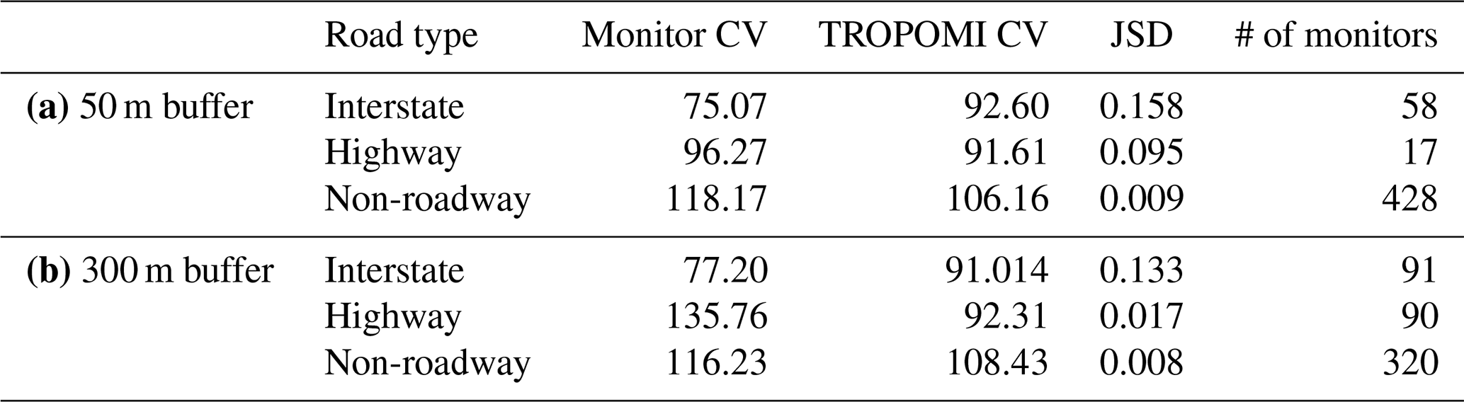
The key differences seen within the JSD across the three monitor classifications are also present in the percentage frequency distributions of NO₂ measured by ground-based monitors and TROPOMI (Fig. S5), with interstate monitors having the lowest alignment (JSD=0.158), highway monitors having better alignment (JSD=0.095), and non-roadway monitors having the best alignment (JSD=0.009). The strong alignment between TROPOMI and monitor distributions in non-roadway regions is consistent with previous studies (Dressel et al., 2022; Kim et al., 2024; Ialongo et al., 2020). This close alignment may be due to the relatively lower NO₂ concentrations, which TROPOMI captures more accurately, compared with regions with higher emissions. These findings further align with previous work showing that TROPOMI tends to underestimate NO₂ in high-pollution areas (such as interstates and highways) but slightly overestimates in areas of lower pollution, such as rural areas (Dressel et al., 2022; Ialongo et al., 2020; Goldberg et al., 2024).

Due to the large jump in NO₂ levels seen within Fig. 1 in the 50–300 m category, we compare the 50 m buffer roadway classifications (Fig. S5; Table 1a) with the 300 m buffer classifications (Fig. S6; Table 1b). Notable differences emerge between distributions, particularly in the highway category, where 73 monitors are added to the highway distribution (increasing from 17 to 90 monitors; Table 1) due to the larger buffer. The alignment between monitor data and TROPOMI observations is significantly improved within the 300 m buffer near highways. This improvement in alignment is likely to be due to the decay of NO₂ with increasing distance from the road (Karner et al., 2010; Kimbrough et al., 2017; Richmond-Bryant et al., 2017). Consequently, the lower surface NO₂ concentrations observed at 300 m are better captured by TROPOMI. This is reflected in Table 1, which shows a substantial reduction in the JSD for highway monitors, from 0.095 in the 50 m buffer to 0.017 in the 300 m buffer (an 82 % increase in alignment at the 300 m buffer).

The differences observed in the highway category with the 300 m buffer may be present, since the distribution includes 73 more monitors than the 50 m buffer, capturing lower NO₂ amounts that are more aligned with TROPOMI's observations. Conversely, the interstate category exhibits less noticeable change, with only 33 additional monitors in the 300 m buffer distribution (increasing from 58 in the 50 m buffer, Table 1a, to 91 in the 300 m buffer, Table 1b). This suggests that the monitors added in the 300 m buffer for interstates measure NO₂ levels similar to those already captured in the 50 m buffer, resulting in little change to the overall distribution.

These results indicate that TROPOMI follows the trend of NO₂ decreasing with increasing distance from roadways that ground-based monitors record and that TROPOMI captures surface concentrations best in winter and at 300+ m away from the traffic source.

3.2 Column–column daily alignment

Here we compare the distributions of NO₂ from TROPOMI and TEMPO with ground-based monitors to assess how well each satellite instrument captures daily variations in NO₂ concentration. Our results indicate that TEMPO consistently aligns more closely with ground-based measurements than TROPOMI, particularly in high-NO₂ areas, such as highways and interstates.

Figure 3 shows the distributions of NO₂, as measured by AQS ground-based monitors (filtered to match valid TROPOMI and TEMPO data), TROPOMI, and TEMPO, separated by road classifications (interstates, highways, and non-roadways) for December 2023 and July 2024. The 13:00 and 14:00 UTC (based on time zone) TEMPO and AQS values were averaged to align with the TROPOMI overpass time of ≈13:30 LT (see Sect. 2.3). The monitor data in each comparison differ, due to the data filtering (see Sect. 2.2 and 2.3). The comparison of frequency distributions reveals how well TEMPO and TROPOMI capture the wide range of ground-based monitor readings across these classifications and time periods.

In December 2023, TEMPO (JSD=0.007) and TROPOMI (JSD=0.021) exhibit distinct differences in how well they capture NO₂ distributions across the various road classifications. Near interstates, TEMPO has a 90th percentile at 18.34×10¹⁵ molec. cm⁻², whereas the TROPOMI 90th percentile is 11.27×10¹⁵ molec. cm⁻². TEMPO aligns more closely with monitor distributions, with a JSD of 0.066, compared with the TROPOMI JSD of 0.145 (Fig. 3). TEMPO has 21.42 % of data points above 11×10¹⁵ molec. cm⁻² for interstate values in December, whereas TROPOMI appears to underestimate the frequency of higher NO₂ levels more, with a cumulative frequency of 10.53 % above that threshold. Near highways, the TEMPO 90th percentile is 14.70×10¹⁵ molec. cm⁻², compared with TROPOMI, with a 90th percentile of 10.06×10¹⁵ molec. cm⁻². The JSD for TEMPO is 0.049 and that for TROPOMI is 0.125 for highway monitors, indicating that TEMPO has much better alignment on highways (Fig. 3). For non-roadway locations, both instruments show very good alignment (TEMPO JSD=0.005; TROPOMI JSD=0.012; Fig. 3) with the monitor data distributions but with TEMPO again being slightly better.

In July 2024, the patterns show greater divergence across road classifications (TEMPO JSD=0.027; TROPOMI JSD=0.049) between the satellite observations and ground-based monitor data, compared with the December 2023 distributions. Near interstates, the TEMPO 90th percentile is 8.46×10¹⁵ molec. cm⁻² and the TROPOMI 90th percentile is 5.58×10¹⁵ molec. cm⁻², with TEMPO aligning more closely (JSD of 0.133 compared with TROPOMI JSD of 0.265; Fig. 3). TEMPO has 17.01 % of data points above 7×10¹⁵ molec. cm⁻² for interstate values in July, whereas TROPOMI appears to underestimate the frequency of higher NO₂ levels more, with a cumulative frequency of 3.61 % above that threshold. Near highways, TEMPO achieves a much better representation of the higher observed NO₂ levels, with a 90th percentile of 9.34×10¹⁵ molec. cm⁻², compared with TROPOMI, with a 90th percentile of 5.32×10¹⁵ molec. cm⁻². The JSD for TEMPO is 0.151 and that for TROPOMI is 0.201 for highway monitors, indicating that TEMPO has better alignment near highways. For non-roadway locations, both instruments show very good alignment (TEMPO JSD=0.024; TROPOMI JSD=0.023; Fig. 3) with the monitor data distributions, with TEMPO and TROPOMI alignment with ground monitors being more comparable than in December 2023.

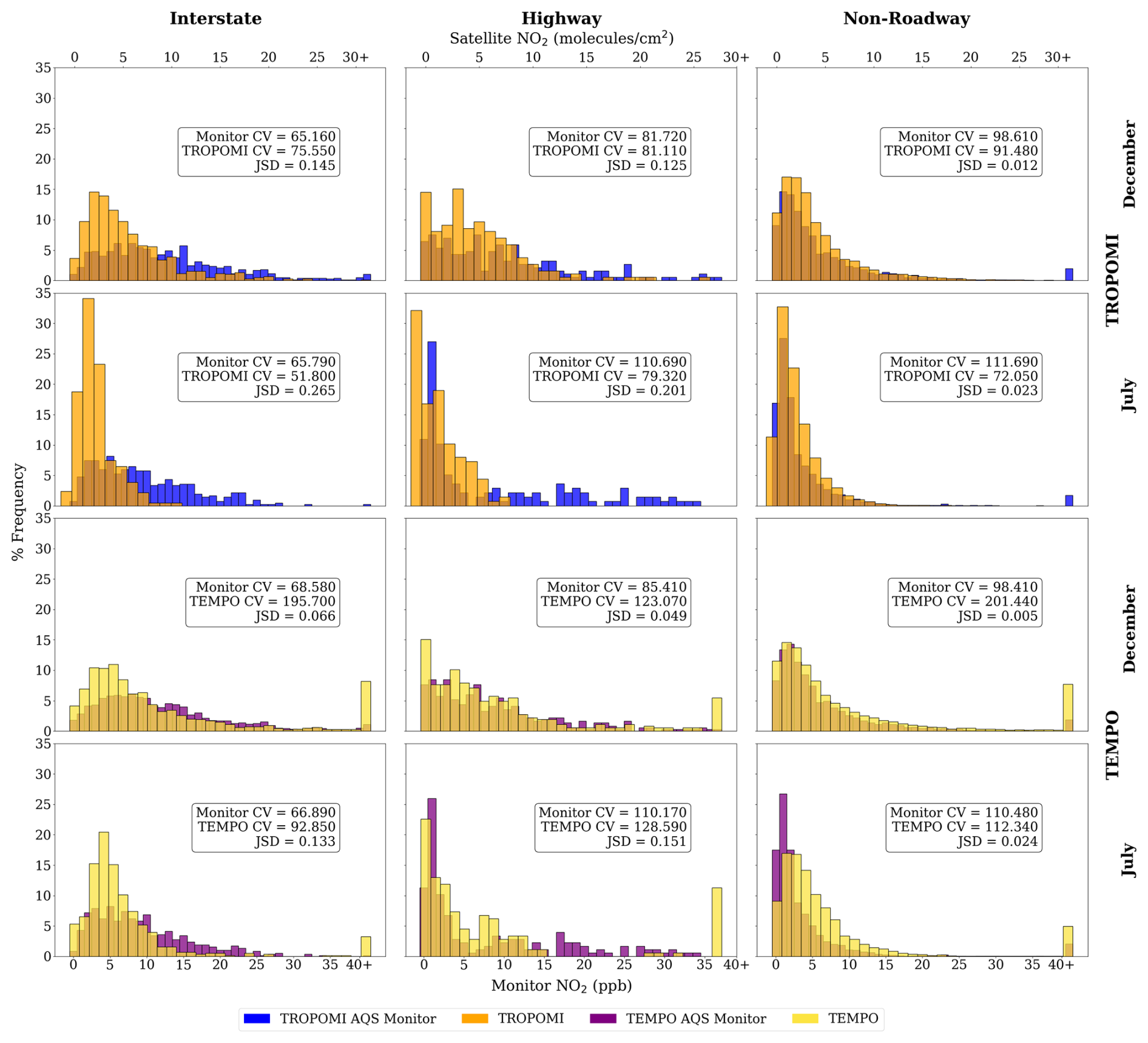
Figure 3 December 2023 and July 2024 at the TROPOMI overpass time (≈13:30 LST): frequency distributions of NO₂, as measured by AQS ground-based monitors filtered to the valid TROPOMI (blue) and TEMPO (purple) and TROPOMI (light orange) and TEMPO (yellow) data for three monitor classifications: interstate, highway, and non-roadway. The x axes indicate the range of NO₂, with the primary lower x axis showing monitor NO₂ concentrations in parts per billion (ppb) and the secondary upper x axis showing TROPOMI NO₂ VCD and TEMPO NO₂ VCD in 10¹⁵ molec. cm⁻². The boxes show the coefficient of variation (CV) and Jensen–Shannon divergence (JSD) for each season and monitor classification.

Throughout both December 2023 and July 2024, TEMPO's improved alignment with ground-based monitors compared with TROPOMI may be attributed to several factors. TEMPO operates from a geostationary orbit, allowing it to take hourly measurements and capture the diurnal variability of NO₂ concentrations more effectively than TROPOMI, which has a single daily overpass time. This high temporal resolution enables TEMPO to better match the timing of NO₂ peaks and fluctuations detected by ground-based monitors, which are also recorded on an hourly basis. Additionally, TEMPO's finer spatial resolution, approximately 2 km in the north–south direction and 4.5 km in the east–west direction, may allow it to capture more localized pollution sources, such as traffic emissions along highways and interstates. This may be why we see such a large difference in alignment in the interstate and highway categories between TEMPO and TROPOMI and very little difference in alignment in the non-road category. In contrast, TROPOMI's 4 km×4 km (re-gridded) resolution and single overpass time may be less effective at capturing these localized variations. TEMPO's finer resolution in one direction and its frequent observations may enable it to more precisely match the spatial and temporal variability detected by ground-based monitors. The consistency of slight underestimation for both instruments in high-pollution areas like highways and interstates suggests challenges in fully capturing elevated NO₂ levels that occur near traffic sources. Overall, this indicates that while TEMPO generally provides a closer approximation of NO₂ distributions compared with TROPOMI, both satellite instruments show limitations, particularly in representing peak concentrations at high-polluting sites.

3.3 Column–surface diurnal alignment

In this section we explore the hourly alignment between monitor and hourly TEMPO distributions at interstate, highway, and non-roadway monitors. We find that TEMPO aligns best with ground monitors around midday and exhibits poorer alignment in the early morning and early evening.

Figure 4 presents the hourly JSD for TEMPO NO₂ measurements compared with ground monitors categorized by interstate (red), highway (orange), and non-roadway (green) monitors for December 2023 (Fig. 4a) and July 2024 (Fig. 4b). The results highlight distinct diurnal patterns across road types and seasons, reflecting the influence of traffic emissions, atmospheric mixing, and insolation.

In December 2023, all monitor categories exhibit similar trends in the early morning, with high JSD values (highway JSD=0.358; interstate JSD=0.331; non-road JSD=0.210) indicative of moderate to poor alignment between TEMPO and ground-based monitors. This pattern, consistent with early morning rush hour emissions and limited atmospheric vertical mixing (Harkey and Holloway, 2024) as well as a decrease in TEMPO's measurement accuracy due to high solar zenith angles in the morning, according to TEMPO documentation (NASA Langley Research Center, 2024), suggests that TEMPO may not capture rapid increases in NO₂ during high-traffic and low-mixing periods. By mid-morning, JSD has decreased for all road types (highway JSD=0.085; interstate JSD=0.067; non-road JSD=0.027), indicative of good alignment, with non-road monitors showing the most significant improvement (87 % increase in alignment). This pattern of better alignment in non-road monitor areas could be attributed to lower NO₂ levels away from major sources of emissions. As the day progresses in December, JSD values for highway and interstate monitors increase steadily (with highways fluctuating more) after 17:00 UTC (≈12:00 LT), with highways increasing in JSD from 0.102 to 0.490 and interstates increasing in JSD from 0.097 to 0.590, indicating worsening alignment in the afternoon and early evening. This pattern may reflect the re-accumulation of NO₂ due to afternoon traffic and the collapse of the boundary layer later in the afternoon (Harkey and Holloway, 2024), as well as the decrease in TEMPO's measurement accuracy in the evening (NASA Langley Research Center, 2024). Non-road monitors show less change in JSD through the day, suggesting that TEMPO alignment is more consistent in non-road monitor areas throughout the rest of the day, only fluctuating in JSD between 0.009 and 0.05.

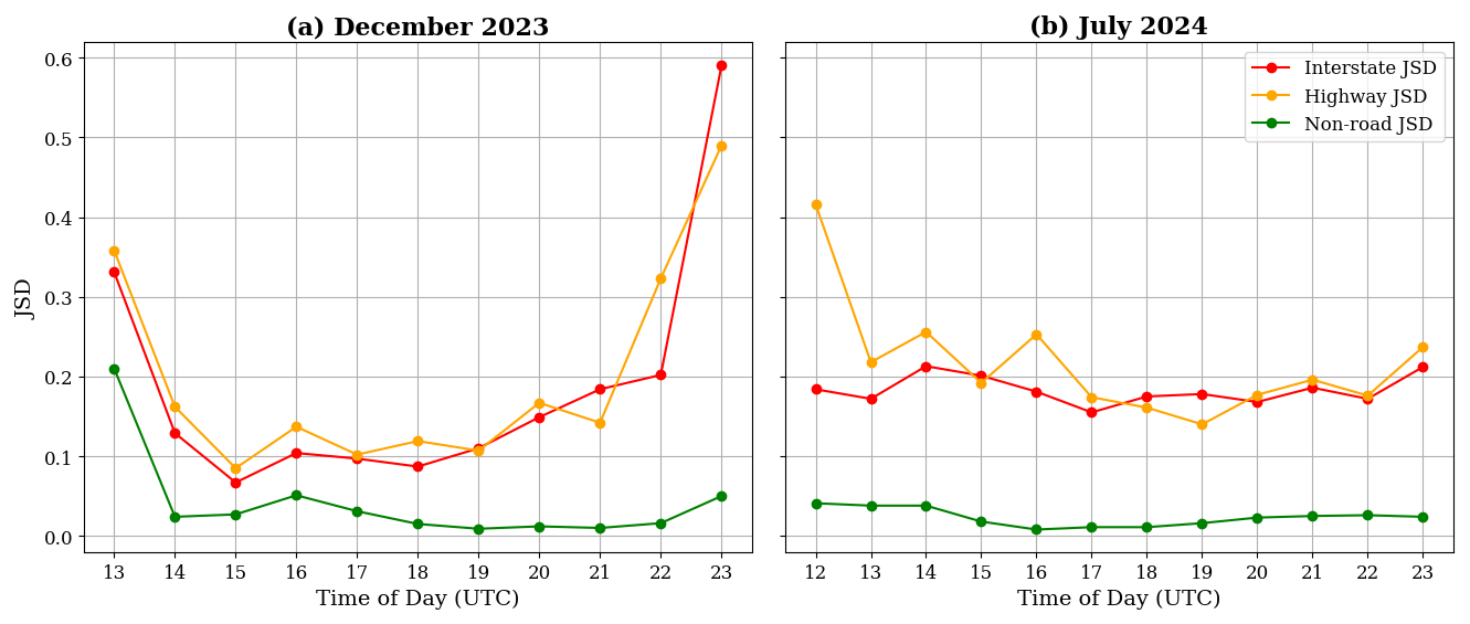
Figure 4 (a) December 2023 and (b) July 2024 hourly (UTC) TEMPO NO₂ Jensen–Shannon divergences at interstate (red), highway (orange), and non-roadway (green) monitor locations.

In July 2024, highway and interstate monitors do not exhibit a clear diurnal pattern, with JSD values fluctuating between 0.14 and 0.416 for highways and 0.155 and 0.212 for interstates throughout the day. Consistent localized traffic emissions and the shorter NO₂ lifetime during the summer suggest a less variable distribution of NO₂. Non-road monitors in July show somewhat worse alignment in the morning (JSD =0.041), with improved agreement during the late morning and early afternoon (JSD ranging between 0.008 and 0.025). The non-road JSD remains fairly constant into the early evening, with alignment decreasing by about 13 %, indicating that sunlight may play a larger role in the alignment in the evening since the sun is at a higher position in the sky during this time in the summer than in the winter (which increases in JSD at this time), enhancing TEMPO's measurement accuracy in the early evening in July.

Both months exhibit their highest JSDs, and worst alignment, in the early morning or early evening hours, which coincide with peak traffic times and the most uncertainty in TEMPO observations caused by the solar zenith angle. The best alignment and lowest JSDs occur sometime near midday (≈10:00 LT to ≈14:00 LT).

The disparity between highways and interstates in TEMPO, where highways generally had the highest JSD, differs from the pattern seen with TROPOMI, where interstates tended to consistently exhibit worse alignment. This suggests that TEMPO's higher spatial and temporal resolution may capture localized sources more effectively, leading to variations in alignment based on the distribution and intensity of NO₂ sources.

4 Conclusions

This study evaluates the distributional alignment among estimates of NO₂ abundance from TROPOMI, TEMPO, and ground monitors to inform the potential of satellite data for both regulatory and public health applications, particularly in informing future NO₂ monitor siting strategies. Several limitations and sources of uncertainty should be considered. Limitations of this analysis include (1) the overrepresentation of AQS monitors in urban areas, (2) the temporal mismatch between satellite and ground measurements, and (3) the fact that the distance-from-roads analysis does not consider other local factors. A key limitation is the overrepresentation of urban areas in the AQS monitoring network, which may bias our results toward urban areas. Since AQS monitors are more densely located in urban regions with high emissions and complex local sources, the results may not fully capture alignment in more rural areas with fewer monitoring stations. Another important consideration is the slight temporal mismatch between satellite and ground-based measurements. TROPOMI provides a single daily observation around 13:30 local solar time, whereas ground monitors and TEMPO record NO₂ concentrations throughout the day. To better align with TROPOMI's overpass, we averaged 13:00 and 14:00 LT TEMPO and ground monitor NO₂ values. Since NO₂ concentrations can change rapidly due to meteorological conditions and emissions variability, this averaging approach may introduce some error in comparisons between TEMPO, TROPOMI, and ground-based measurements. The classification of monitors by distance from roads is based on buffer analysis, which does not account for local factors, such as wind direction, terrain, proximity to industry, and traffic density, all of which influence NO₂ dispersion. Despite these uncertainties, our findings highlight patterns in column–surface NO₂ agreement and demonstrate the potential for satellite data to complement ground-based monitoring.

The Jensen–Shannon divergence (JSD) offers a robust and interpretable metric for comparing the alignment and similarity of NO₂ distributions. Its symmetry and bounded range allowed us to evaluate the degree of similarity between satellite and monitor NO₂ values across different spatial and temporal scales, providing a clear quantitative framework for assessing the similarity of two different instruments.

Past studies comparing surface and satellite NO₂ have found temporal correlation of daily values at individual sites ranging from r=0.61 to r=0.69 (Lamsal et al., 2014, 2015), monthly and seasonal values at individual sites ranging from r= 0.67 to r= 0.90 (Griffin et al., 2019; Yu and Li, 2022; Harkey and Holloway, 2024; Dressel et al., 2022; Xu and Xiang, 2023; Lamsal et al., 2015), and annual average values at sites ranging from r=0.68 to r=0.93 (Zhang et al., 2018; Lamsal et al., 2015; Goldberg et al., 2021; Kim et al., 2024; Bechle et al., 2013; Lee et al., 2023). Here, r refers to the Pearson correlation coefficient, which measures the strength and direction of a linear relationship between variables. In some cases, these comparisons adjusted column values to the surface (e.g., Lamsal et al., 2014) and/or adjusted ground monitors to reduce the error in chemiluminescent detection of NO₂ (e.g., Lamsal et al., 2015; Bechle et al., 2013). Using similar methods, TROPOMI tends to show better agreement with annual AQS NO₂ than does the Ozone Monitoring Instrument (OMI), e.g., r=0.81 using TROPOMI (Goldberg et al., 2021) versus r=0.68 from OMI (Lamsal et al., 2015). Off-road AQS monitors tend to show better agreement with satellite data than near-road AQS monitors, e.g., r=0.81–0.87 at non-near-road sites versus r=0.64–0.74 at near-road sites (Kim et al., 2024). The underestimation of estimated near-surface NO₂ near roads and localized sources is a recurring issue in OMI and TROPOMI NO₂ VCDs (Dressel et al., 2022; Goldberg et al., 2024; Ialongo et al., 2020).

In this study, we find a pattern of decreasing NO₂ with increasing distance from traffic sources, which is consistent with the findings of previous studies (Kimbrough et al., 2017; Karner et al., 2010; Richmond-Bryant et al., 2017). While ground-based monitors and TROPOMI satellite data may differ with proximity to roadways, particularly within 50 m, their measurements still follow the same overall trend. This convergence with increasing distance may be due to the reduction of localized near-road emissions and the broader atmospheric mixing captured more effectively by satellite observations at greater distances from roads. Using a larger buffer distance from roads (300 m instead of 50 m) improves the alignment between TROPOMI and monitor data, especially for highway monitor locations (JSD decreases by ≈82 %). The overall trend reflects the well-established gradient of declining NO₂ levels with increasing distance from traffic sources, and TROPOMI's ability to capture this trend, even if the specific values differ from AQS monitors in the near-road environment. Our findings indicate that TROPOMI tends to slightly underestimate surface NO₂ concentrations in areas with high traffic, such as interstates and highways, due to its spatial resolution and full-column measurements, which smooth out localized, ground-level pollution peaks captured by ground monitors. This is most evident in interstate monitors, where the JSD reveals the greatest divergence between satellite and monitor data (JSD=0.158). These results are consistent with prior studies (Dressel et al., 2022; Kim et al., 2024; Ialongo et al., 2020), which also found that satellite instruments are less effective at capturing high NO₂ events near localized sources like traffic. The distributional alignment improves in non-roadway monitors (JSD=0.009), where NO₂ levels are lower, and there are usually fewer localized sources of pollution. The lower pollution levels in these areas allow TROPOMI to more accurately reflect the conditions captured by ground-based monitors, leading to lower JSD values and therefore better alignment. This trend suggests that TROPOMI may be particularly useful for monitoring air quality in rural or less-polluted regions where ground monitors are sparse or absent.

Seasonality plays a critical role in the similarity of satellite and monitor data. Winter consistently shows the best alignment (JSD=0.010), with the TROPOMI distribution capturing nearly the full gradient of NO₂ seen within the ground-based monitor distribution. This probably reflects the longer atmospheric lifetime of NO₂ in winter, which allows for better vertical mixing and less spatial variability (Harkey et al., 2015; Boersma et al., 2009; Shah et al., 2020). In contrast, summer shows the worst alignment (JSD=0.035), which is probably due to the shorter lifetime of NO₂ and increased photochemical activity during warmer months, causing greater discrepancies between localized surface measurements and the satellite column. Similar conclusions were reached by previous studies (Shah et al., 2020; Karagkiozidis et al., 2023), indicating that seasonality is a crucial factor in assessing satellite performance for regulatory purposes. These seasonal differences underscore the need for considering temporal factors when evaluating the use of satellite data for monitor siting and NO₂ regulation.

The integration of TEMPO data in this study highlights TEMPO's potential to advance our understanding of NO₂ distributions, especially when compared with TROPOMI. TEMPO's ability to provide hourly measurements at a finer spatial resolution offers significant advantages in capturing diurnal NO₂ patterns and detecting localized pollution events. Our findings from December 2023 and July 2024 at the TROPOMI overpass time (≈13:30 LST) demonstrate that TEMPO captures the wide range of surface NO₂ measurements better than TROPOMI, especially at higher NO₂ levels. TEMPO's JSDs are almost always lower than TROPOMI's, with JSDs ranging from 0.005 to 0.151 and TROPOMI's JSDs ranging from 0.012 to 0.265. This improvement in alignment with ground monitors could be attributed to TEMPO's better spatial and temporal resolution.

We also find that TEMPO is best at capturing ground-level NO₂ amounts around midday (≈10:00 to ≈14:00 LT). This could be due to the lower traffic levels and therefore lower pollution levels during this time period, as well as a lower solar zenith angle, allowing TEMPO to have more accurate measurements. However, challenges remain in completely capturing high NO₂ levels during peak traffic times and accurately capturing NO₂ during high solar zenith angles in the morning and evening across monitor classifications. These results underscore the influence of spatial resolution, time of day, and measurement frequency on the ability of satellite instruments to align with ground-based NO₂ measurements. Future research should build upon these insights by incorporating longer time periods and multiple years of data as more TEMPO data become available to study long-term TEMPO distributions. The enhanced temporal and spatial resolution of TEMPO, alongside its comparison with other instruments like TROPOMI, provides valuable context for understanding the dynamics of NO₂ pollution, especially how it varies throughout the day. Spatially contiguous satellite products and our analysis of air quality variability offer the potential to support air quality managers and public health analysis.