Observational constraints suggest a smaller effective radiative forcing from aerosol–cloud interactions

The effective radiative forcing due to aerosol–cloud interactions (ERFaci) is difficult to quantify, leading to large uncertainties in model projections of historical forcing and climate sensitivity. In this study, satellite observations and reanalysis data are used to examine the low-level cloud radiative responses to aerosols. While some studies assume that the activation rate of cloud droplet number concentration (N_d) in response to variations in sulfate mass concentration (${{\mathrm{SO}}_{\mathrm{4}}}^{\mathrm{2}-}$) has a one-to-one relationship, we find this assumption to be incorrect. Our analysis estimates a global mean activation rate of 0.35 ± 0.17 (90 % confidence) and demonstrates that explicitly accounting for the activation rate is crucial for accurate ERFaci estimation. This is corroborated through a “perfect-model” cross-validation using state-of-the-art climate models. Our results suggest a smaller and less uncertain value of the global ERFaci (−0.32 ± 0.21 W m⁻² for ${{\mathrm{SO}}_{\mathrm{4}}}^{\mathrm{2}-}$, 90 % confidence) than recent climate assessments (e.g., −0.93 ± 0.7 W m⁻², 90 % confidence), indicating that ERFaci may be less impactful than previously thought. Our results are also consistent with observationally constrained estimates of total cloud feedback and recent estimates that models with weaker ERFaci better match the observed hemispheric warming asymmetry over the historical period.

1 Introduction

Anthropogenic aerosols impact the Earth's radiation balance at the top of the atmosphere, with this perturbation quantified as radiative forcing (e.g., Boucher et al., 2013; Raghuraman et al., 2021; Kramer et al., 2021). They directly alter the radiation budget by scattering and absorbing solar radiation and indirectly influence it by serving as cloud condensation nuclei (CCN), which modifies cloud properties and can extend their duration. The increase in aerosol concentration leads to smaller cloud droplets and higher cloud albedos, known as the “Twomey effect” (e.g., Twomey, 1977), enhancing the negative radiative forcing due to aerosol–cloud interactions (RFaci). Additionally, aerosols affect cloud microphysical properties (e.g., Albrecht, 1989; Pincus and Baker, 1994), such as reducing precipitation, which increases cloud liquid water path (LWP), lifetime, and fraction, a process termed cloud adjustment (CA). Thus, together, RFaci and CA are intrinsically interconnected through the cloud droplets (Mülmenstädt and Feingold, 2018) and constitute the effective radiative forcing from aerosol–cloud interactions (ERFaci). ERFaci is highly uncertain and often larger than the direct radiative impact of aerosols (Forster et al., 2007; Zelinka et al., 2014; Smith et al., 2020a).

Estimating the ERFaci, especially in low-level clouds which are the dominant contributor of aerosol–cloud interactions to ERFaci (Christensen et al., 2016; Bellouin et al., 2020; Forster et al., 2021), is critical for accurately identifying cloud feedback mechanisms and determining climate sensitivity (Rosenfeld, 2006; Boucher et al., 2013; Sherwood et al., 2020). Our study provides quantitative insights into the ERFaci using both satellite observations and reanalysis data. A key component of our analysis is the activation rate, which serves as a metric for assessing the actual impact of aerosols on cloud droplet number concentrations (N_d). In some studies, the activation rate is not explicitly incorporated into the estimation process of ERFaci, as it is implicitly assumed to have a one-to-one relationship (e.g., Chen et al., 2014; Christensen et al., 2016; Douglas and L'Ecuyer 2020; Wall et al., 2022, 2023). Our results suggest the importance of considering the activation rate when evaluating the interactions between aerosols and clouds. To evaluate the robustness of our results, we conduct a “perfect-model” cross-validation using Coupled Model Intercomparison Project Phase 6 (CMIP6) simulations. This form of cross-validation is widely used in statistics and machine learning to assess the generalizability of predictive models and prevent overfitting (Wenzel et al., 2016; Knutti et al., 2017; Brunner et al., 2020). Through this approach we demonstrate that explicitly including the activation rate is essential to improving the accuracy of ERFaci estimates.

In the main text, our analysis primarily focuses on sulfate mass concentration (${{\mathrm{SO}}_{\mathrm{4}}}^{\mathrm{2}-}$) at 925 hPa as an aerosol proxy, derived from the Modern-Era Retrospective Analysis for Research and Applications version 2 (MERRA-2; Randles et al., 2017; Gelaro et al., 2017). Sulfate aerosol is recognized as a dominant contributor to ERFaci as well as cloud droplet formation, among other aerosol types such as black carbon, organic carbon, sea salt, and dust (Charlson et al., 1992; Stevens, 2015; McCoy et al., 2018). Additionally, results derived from satellite measurements of the aerosol index (AI) from Moderate Resolution Imaging Spectroradiometer (MODIS; Platnick et al., 2015a, b) also show a high degree of consistency.

2 Results

2.1 Activation rate

Some approaches to estimate the ERFaci with aerosol concentrations have operated under a key assumption: the natural logarithm of aerosol concentration correlates proportionally with the natural logarithm of cloud droplet number concentration (e.g., Chen et al., 2014; Christensen et al., 2016; Douglas and L'Ecuyer, 2020; Wall et al., 2022, 2023). This relationship, commonly referred to as the activation rate, quantifies the efficiency with which aerosol particles convert into cloud droplets. The hypothesized cause–effect relationship between aerosols and clouds is important to understand and to be dealt in the process of aerosol–cloud interactions, as it involves an increase in CCN leading to an increase in N_d, which subsequently influences cloud properties. To verify the key assumption while accounting for environmental influences, we performed cloud controlling factor (CCF) analysis (Appendix A6). Figure 1 illustrates the regression coefficients between ln(N_d) and ln(${{\mathrm{SO}}_{\mathrm{4}}}^{\mathrm{2}-}$), with all other environmental predictors held constant. Our results show that, in most regions, these coefficients are positive but less than 1, underscoring that not all sulfate in the atmosphere is converted into cloud droplets. On a global scale, the mean activation rate is 0.35, indicating that sulfate aerosol activation is less efficient than a one-to-one conversion. Regions with shallow cumulus clouds, such as the central Pacific, show notably weaker $\partial \ln \left(N_{\mathrm{d}}\right)/\partial \ln \left({{\mathrm{SO}}_{\mathrm{4}}}^{\mathrm{2}-}\right)$ coefficients, while areas with stratocumulus clouds, like those off the coasts of continents, display relatively stronger positive regression coefficients (Fig. 1). This variation may be attributed to differences in local environmental conditions and the role of aerosols in which these clouds occur (e.g., Douglas and L'Ecuyer, 2019, 2020). Repeating our analysis using AI yields somewhat different results with those for ${{\mathrm{SO}}_{\mathrm{4}}}^{\mathrm{2}-}$ though still showing strong positive regression coefficients near continental coasts, with a global mean of 0.21 (Fig. S1 in the Supplement). The differences in regression coefficients observed for $\partial \ln \left(N_{\mathrm{d}}\right)/\partial$ln(AI) may be attributed to the use of column-integrated quantities, AI from MODIS, which do not account for the vertical structure of aerosols. Consequently, they may not accurately represent aerosol concentrations at cloud base height.

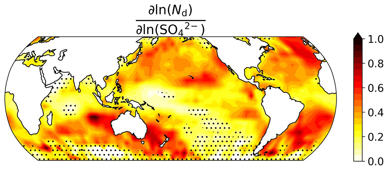
Figure 1 Regression coefficient map of the activation rate of cloud droplet number concentration (N_d) in response to variations in sulfate aerosol mass concentration (${{\mathrm{SO}}_{\mathrm{4}}}^{\mathrm{2}-}$) for the period January 2003 to December 2019, derived from cloud controlling factor (CCF) analysis (Appendix A6). The color scale indicates the magnitude of sensitivity, where an increase in ${{\mathrm{SO}}_{\mathrm{4}}}^{\mathrm{2}-}$ corresponds to an increase in N_d. Areas with stippling indicate where the changes are not statistically different from zero at the 95 % confidence level using Student's t test.

2.2 Observationally constrained ERFaci

We now proceed to estimate the observationally constrained ERFaci (ERFaci_obs), considering two scenarios: one with and the other without the inclusion of the activation rate. The basic form of ERFaci_obs following Wall et al. (2022), where the activation rate is not explicitly included, can be expressed as follows:

$$\begin{array}{}\text{(1)}& \mathrm{ERFaci}\mathrm{\_}\mathrm{obs}\approx {\displaystyle \frac{\partial \mathrm{CRE}\mathrm{\_}\mathrm{lcld}}{\partial \ln \left(X\right)}}\times \mathrm{\Delta }\ln \left(X\right),\end{array}$$

where CRE_lcld represents the cloud radiative effect from non-obscured (non-overlapped) low-level clouds, obtained from the Clouds and the Earth's Radiant Energy System (CERES) FluxByCldTyp Ed. 4.1 dataset (Sun et al., 2022), and X represents either ${{\mathrm{SO}}_{\mathrm{4}}}^{\mathrm{2}-}$ or AI. The right-hand side of the equation consists of two main parts: one is the susceptibility of the low cloud radiative effect to variations in aerosol concentrations, derived from CCF analysis while holding other environmental conditions constant (Appendix A6), and the other is the changes in aerosol concentrations from pre-industrial (PI) to present-day (PD). Due to the lack of observational data on PI aerosol concentrations, we employ the outputs of CMIP6 historical experiments. As expected, changes in sulfate mass concentration exhibit distinctive spatial patterns characterized by interhemispheric asymmetry, with particularly large values in proximity to major industrial regions on the Eurasian and North American continents (Fig. 2a).

In light of Fig. 1, the basic form of ERFaci_obs in Eq. (1) can be expanded to incorporate the influence of the activation rate by accounting for the interactions between aerosols and cloud droplet formation. This modified equation can be expressed as follows:

$$\begin{array}{}\text{(2)}& \mathrm{ERFaci}\mathrm{\_}\mathrm{obs}\approx \left({\displaystyle \frac{\partial \mathrm{CRE}\mathrm{\_}\mathrm{lcld}}{\partial \ln \left(N_{\mathrm{d}}\right)}}\times {\displaystyle \frac{\partial \ln \left(N_{\mathrm{d}}\right)}{\partial \ln \left(X\right)}}\right)\times \mathrm{\Delta }\ln \left(X\right),\end{array}$$

where the low cloud susceptibility is now the product of two terms: the susceptibility of low cloud CRE to N_d and the activation rate of X to N_d.

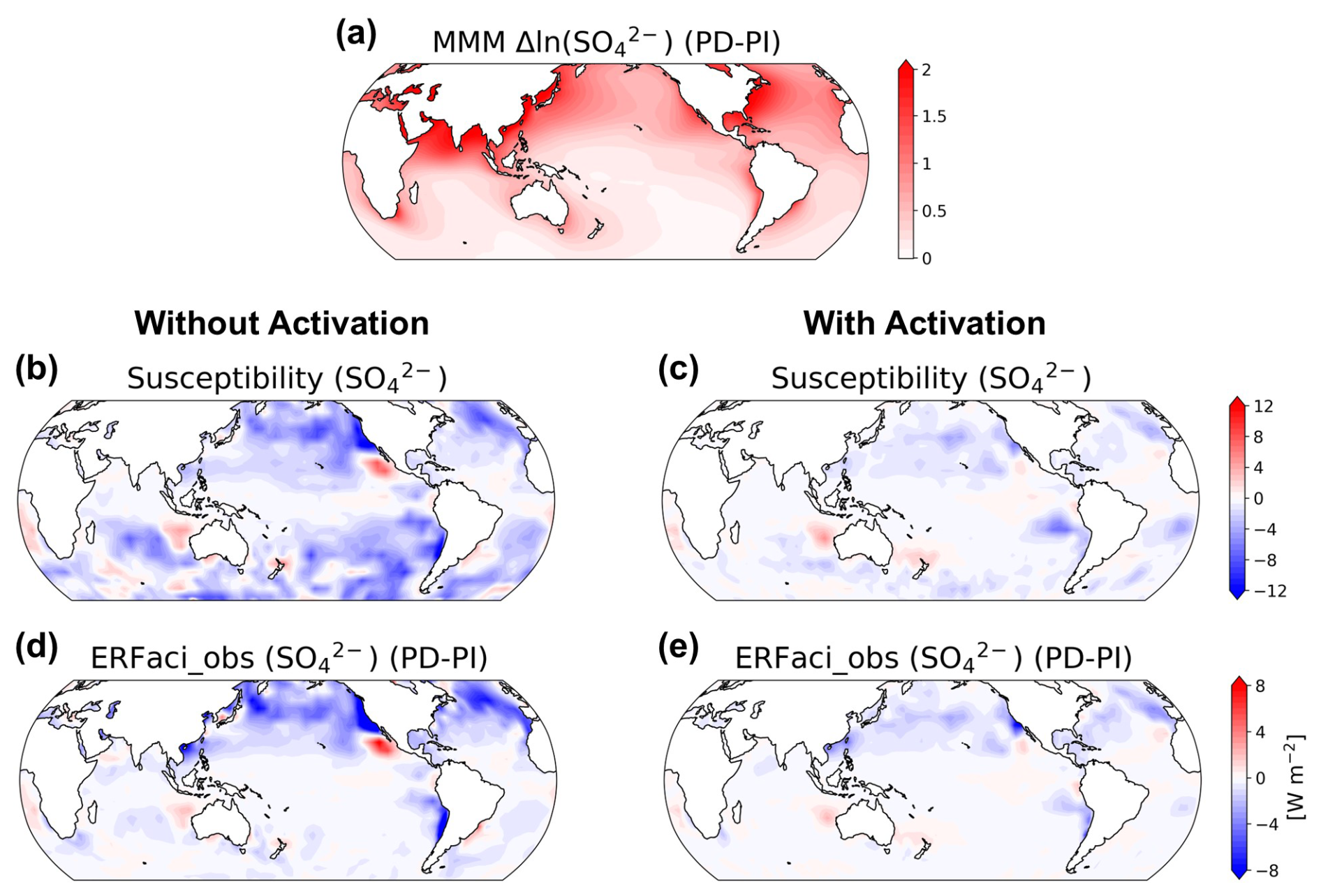
Figure 2 Spatial distribution of ERFaci_obs components and the estimated ERFaci_obs differentiated by the consideration of the activation rate. (a) Multi-model mean (MMM) of changes in ${{\mathrm{SO}}_{\mathrm{4}}}^{\mathrm{2}-}$ between pre-industrial (PI) and present-day (PD) periods. In total, 13 models are used for this analysis (Table S1 in the Supplement). (b, c) Susceptibility of low cloud radiative effect to ${{\mathrm{SO}}_{\mathrm{4}}}^{\mathrm{2}-}$ derived from CCF analysis using observational and reanalysis data (Appendix A6). (d, e) Observationally constrained ERFaci for ${{\mathrm{SO}}_{\mathrm{4}}}^{\mathrm{2}-}$ estimated by multiplying the susceptibility with the changes in ${{\mathrm{SO}}_{\mathrm{4}}}^{\mathrm{2}-}$.

Our analysis reveals pronounced differences in susceptibility in how low cloud radiative effects respond to variations in aerosol concentrations across the globe depending on whether the activation rate is considered or not. The inclusion of the activation rate in our analysis considerably diminishes the sensitivity of clouds to aerosols (Fig. 2b vs Fig. 2c). Noticeable decreases in susceptibility are captured in mid-latitudes and in subtropical regions where low clouds are dominant. This also indicates that the coefficient of ∂ln(CRE_lcld)/∂ln(${{\mathrm{SO}}_{\mathrm{4}}}^{\mathrm{2}-}$) without the activation rate is partially attributable to factors other than the N_d-mediated mechanism (Gryspeerdt et al., 2016).

Both methods of estimating ERFaci_obs show that an increase in aerosol concentration correlates with a negative cloud radiative adjustment that is especially prevalent in areas dominated by low clouds (Fig. 2d, e). However, due to the reduced susceptibility, the estimated ERFaci_obs is markedly smaller when activation is explicitly accounted for (Fig. 2e) than when it is not (Fig. 2d). Specifically, the global ERFaci_obs is ∼ 64 % smaller with activation (−0.32 W m⁻²) than without (−0.88 W m⁻²). Similar results are obtained if one uses AI instead of ${{\mathrm{SO}}_{\mathrm{4}}}^{\mathrm{2}-}$ as the measure of aerosol concentration (Fig. S2d, e).

2.3 Perfect-model cross-validation

In this section, we perform a perfect-model cross-validation exclusively using CMIP6 simulations to assess which of the two approaches – considering the activation rate or not – is more accurate. Specifically, in single-forcing (aerosol-only) experiments from the Radiative Forcing Model Intercomparison Project (RFMIP; Pincus et al., 2016), each model is sequentially treated as the “truth”, with its ERFaci considered the “true” value. Meanwhile, the same model from historical simulations, assumed to be a pseudo-observation, estimates ERFaci for comparison with the true ERFaci. The resulting root mean square error (RMSE) provides a quantitative measure of the accuracy of the ERFaci estimates.

As an initial step in the perfect-model test, single-forcing (aerosol-only) CMIP6 simulations are used to establish the true ERFaci for each model, referred to as ERFaci_true, which provides a benchmark for assessing the accuracy of the ERFaci estimated from the monthly outputs of CMIP6 historical experiments using Eqs. (1) and (2), where the model is treated as a pseudo-observation, and the estimate is referred to as ERFaci_est. Because the number of CMIP6 models that provide single-forcing (aerosol-only) simulations for ERFaci_true is limited, we also explore another technique for estimating ERFaci introduced by Soden and Chung (2017; referred to as ERFaci_SC17) that has been previously shown to agree well with ERFaci_true (Chung and Soden, 2017). For more details on the estimation of these three different ERFaci using CMIP6 model outputs, please refer to Appendix A7. A comparison, for the perfect-model test, of ERFaci_est with both ERFaci_true and ERFaci_SC17 is provided below.

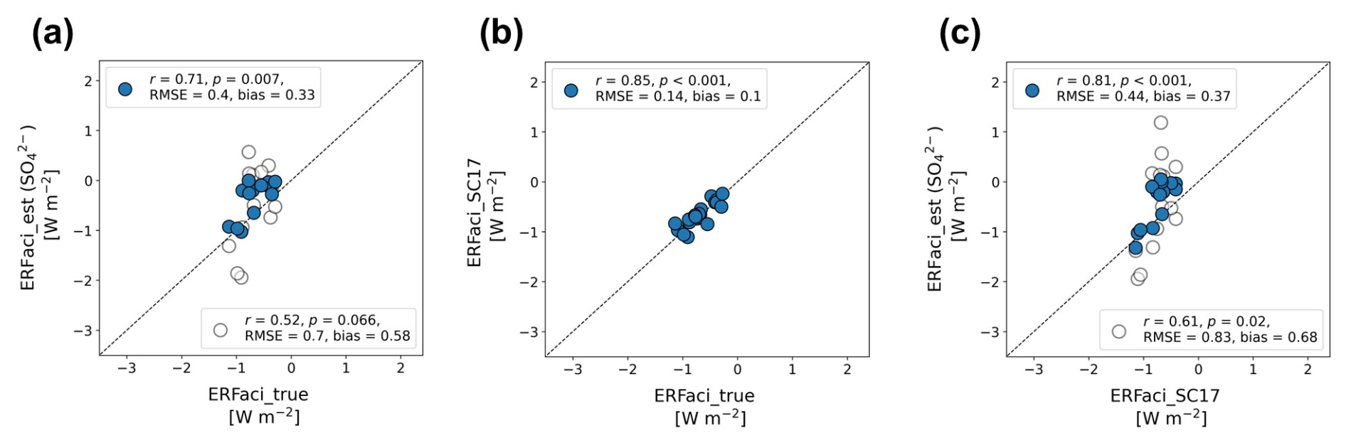
Figure 3 Perfect-model cross-validation analysis of global-mean ERFaci estimates. (a) ERFaci_true versus ERFaci_est, which is estimated by simplified version of Eqs. (1) and (2) with ${{\mathrm{SO}}_{\mathrm{4}}}^{\mathrm{2}-}$ as the aerosol proxy (Appendix A7); (b) ERFaci_true versus ERFaci estimates obtained using the method proposed by Soden and Chung (2017; SC17); and (c) ERFaci_SC17 versus ERFaci_est. Filled blue circles represent estimates where the activation rate is considered, and open grey circles represent estimates without activation rate consideration. The correlation coefficient (r), associated p value (p), root mean square error (RMSE), and bias are displayed in the upper left corner for the filled blue circles and in the lower right for the open grey circles in each panel. Bias is defined as the mean absolute difference from the 1:1 reference line, depicted by a dashed line. All panels have identical x and y axis ranges to highlight the variance among the estimation methods. Higher r values, lower RMSE, and minimal bias indicate consistency in ERFaci estimates across different estimation methods using CMIP6 models.

Figure 3 illustrates the correlation between ERFaci_true and two alternative approaches derived from CMIP6 model output. The estimates of ERFaci_est that omit the activation rate fail to replicate the true ERFaci values accurately, with RMSE of 0.7 W m⁻² and bias of 0.58 W m⁻². Conversely, incorporating an explicit activation rate into the ERFaci estimates provides better agreement with ERFaci_true, reducing both the RMSE and bias by around 43 % (Fig. 3a).

ERFaci_SC17 exhibits the best agreement with ERFaci_true, with markedly smaller RMSE (0.14 W m⁻²) and bias (0.1 W m⁻²) (Fig. 3b). This consistency allows us to expand the sample size of CMIP6 models, with which we can evaluate ERFaci_est by using ERFaci_SC17 as a surrogate for ERFaci_true (Fig. 3c). This expanded cross-validation once again highlights the importance of including the activation rate in ERFaci estimates, as it reduces both the RMSE and bias in ERFaci_est by over 45 %. Substituting AI for ${{\mathrm{SO}}_{\mathrm{4}}}^{\mathrm{2}-}$ in the calculation of ERFaci_est yields similar results, which reduces RMSE up to 36 % (Fig. S3). Our perfect-model cross-validation analysis with idealized model experiments from CMIP6 leads us to conclude that the inclusion of the activation rate is essential for accurate estimates of ERFaci.

2.4 Comparison with previous ERFaci estimates

Now, we compare our observationally constrained estimates of ERFaci_obs with those previously estimated. To estimate global-average ERFaci_obs from our domain-average ERFaci_obs, we multiply our domain estimate by a scalar multiplier, γ, which represents the ratio of multi-model mean of global-average ERFaci_true to domain-average ERFaci_true (Appendix A9). Our global estimates with inclusion of activation rate yield an ERFaci of −0.32 ± 0.21 W m⁻² for ${{\mathrm{SO}}_{\mathrm{4}}}^{\mathrm{2}-}$ and $-\mathrm{0.19}\pm \mathrm{0.17}$ W m⁻² for AI (Fig. 4). These values are at the higher bound (less negative) when compared with the ERFaci estimate reported in the Sixth Assessment Report of the Intergovernmental Panel on Climate Change (IPCC; Forster et al., 2021) and the estimate proposed by the World Climate Research Program (WCRP; Bellouin et al., 2020). However, it is worth noting that the ERFaci from WCRP has a highly skewed distribution, with its highest probability occurring around −0.4 W m⁻², which is consistent with our observational estimates (Fig. 4). Given the multiple lines of evidence introduced by the WCRP, which employs a process-oriented approach to bound ERFaci, our estimates offer further evidence to support estimates on the higher end (less negative) of their range. Furthermore, these constrained ERFaci_obs values are also consistent with the recent estimates provided by Wang et al. (2021), which demonstrate that models exhibiting weaker ERFaci are more in line with the observed variations in global mean surface temperature as well as hemispheric warming asymmetry during the historical period.

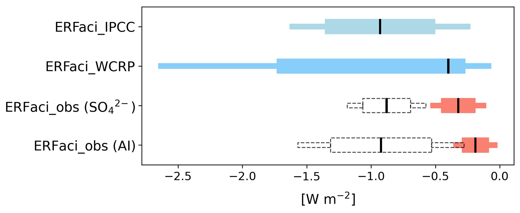
Figure 4 Estimates of globally averaged ERFaci values, including those from the IPCC Sixth Assessment Report, from the WCRP assessment, ERFaci_obs for ${{\mathrm{SO}}_{\mathrm{4}}}^{\mathrm{2}-}$, and ERFaci_obs for AI. The ERFaci_obs estimates considering activation rate are shown in red, while those not considering activation rate are displayed by dashed grey lines. Thin and thick bars represent the 90 % and 66 % confidence intervals (CI), respectively, except for the WCRP estimate of ERFaci, which shows 68 % CI for the thick bar. The black vertical lines indicate the best estimate of each ERFaci. The ERFaci estimate from the IPCC represents the assessment based on observational evidence alone.

As we emphasized the pronounced impact of including the activation rate in the ERFaci estimation process, with this inclusion, the ERFaci_obs values are approximately one-third for ${{\mathrm{SO}}_{\mathrm{4}}}^{\mathrm{2}-}$ and one-fifth for AI of those estimated without considering the activation rate, respectively ($-\mathrm{0.88}\pm \mathrm{0.31}$ W m⁻² for ${{\mathrm{SO}}_{\mathrm{4}}}^{\mathrm{2}-}$ and −0.92 ± 0.65 W m⁻² for AI).

2.5 Implications for cloud feedback

Our observational estimate of ERFaci is on the higher end (less negative) compared to previous estimates. This finding also has implications for our understanding of cloud feedback mechanisms. Following Wang et al. (2021), we compare the CMIP6 historical simulations of ERFaci across different climate models with their corresponding values of total cloud feedback, which are derived from the regression slope of total cloud radiative response to global-mean surface temperature anomalies from the abrupt-4xCO₂ experiment (Fig. 5). For this analysis, we use the ERFaci_SC17 since it ensures the widest possible selection of climate models (Table S1). Among the models we assessed, we identified a subset of 15 that we termed “GOOD HIST” models (Appendix A4). These models are characterized by their small discrepancies in simulating global-mean historical surface warming when compared to the GISS Surface Temperature Analysis (GISTEMP v4; Lenssen et al., 2019) observational data, indicating a higher reliability in their historical climate simulations. Within this subset, a strong negative correlation ($r=-\mathrm{0.85}$, p<0.001) exists between ERFaci_SC17 and the total cloud feedback, which is much more pronounced than in the remaining models ($r=-\mathrm{0.31}$, p=0.042). The strong correlation in the GOOD HIST models highlights the compensation that occurs between historical aerosol forcing and cloud feedback in order for models to reproduce the observed historical global-mean temperature.

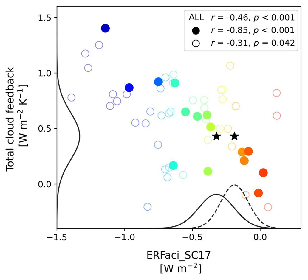
Figure 5 Correlation between global-mean ERFaci estimates obtained using the method proposed by Soden and Chung (2017; SC17), aimed at expanding the model availability, and the globally averaged total cloud feedback as determined by the corresponding models. Each dot represents a single model. The colors from red to blue indicate weak ERFaci models to strong negative ERFaci models. Filled circles represent the 15 GOOD HIST models that align more closely with historical observations of global-mean surface warming, whereas open circles denote the remaining models (Appendix A4). Correlation coefficients (r) and their associated p values (p) for the entire models, the GOOD HIST models, and remaining models are shown in the upper right corner. The probability density functions (PDFs), showing the 90 % confidence intervals for observationally constrained ERFaci from sulfate mass concentration (${{\mathrm{SO}}_{\mathrm{4}}}^{\mathrm{2}-}$; solid line) and the aerosol index (AI; dashed line) when the activation rate is accounted for, are plotted along the x axis, while the PDF for observationally constrained total cloud feedback (solid line), derived from Ceppi and Nowack (2021), is plotted on the y axis (amplitudes scaled arbitrarily). Stars denote the best estimates of the PDFs, signifying the most probable values within the distributions.

Also shown are the probability density functions for the observation-based estimates of ERFaci_obs, taking into account the activation rate, and utilizing both ${{\mathrm{SO}}_{\mathrm{4}}}^{\mathrm{2}-}$ and the AI. Alongside, we also consider the observationally constrained estimates of total cloud feedback, which a recent study (Ceppi and Nowack, 2021) has quantified at 0.43 ± 0.35 W m⁻² K⁻¹ (90 % confidence). These distributions help illustrate that our constraints on ERFaci fall within the realistic bounds of total cloud feedback strength. The best estimates, which show the highest probability (indicated by stars), also align with those from the GOOD HIST models and support the validity of our constraints. Notably, our analysis reveals that models with weaker (less negative) ERFaci and moderately low total cloud feedback agree best with observationally constrained values.

3 Conclusions

Our study offers critical insights into the quantification of the effective radiative forcing from aerosol–cloud interactions (ERFaci), a key source of uncertainty in understanding climate sensitivity. By integrating both satellite observations and reanalysis data, we focus on the activation rate of cloud droplet number concentration in response to aerosol concentration variations, estimated globally at 0.35 ± 0.17 for ${{\mathrm{SO}}_{\mathrm{4}}}^{\mathrm{2}-}$ and 0.21 ± 0.23 for AI (90 % confidence), providing a more sophisticated understanding of the impact of aerosols on low-level clouds. Our findings, validated through the perfect-model cross-validation using CMIP6 model simulations, reveal a less negative global ERFaci estimate (−0.32 ± 0.21 W m⁻² for ${{\mathrm{SO}}_{\mathrm{4}}}^{\mathrm{2}-}$ and −0.19 ± 0.17 W m⁻² for AI, 90 % confidence) than previously reported (e.g., −0.93 ± 0.7 W m⁻² in IPCC AR6, 90 % confidence).

However, we recognize that the error bars on our constraints may not fully capture the broader uncertainties present in climate assessments. Different methodologies employing multiple observational constraints (Regayre et al., 2023) and energy balance constraints (Albright et al., 2021) suggest a wider ERFaci uncertainty range, from −0.9 to −0.1 and −0.9 to −0.2 W m⁻², respectively (90 % confidence). Our reliance on selective satellite observations, reanalysis data, and model outputs may inherently limit our uncertainty range. Despite employing the optimal N_d filtering method in our analysis, which aligns well with aircraft in situ observations (Appendix A3), there remain uncertainties in N_d derived from cloud optical depth and effective radius retrievals from MODIS satellite observations. Thus, we estimate ERFaci using two additional cloud droplet filtering methods introduced in Gryspeerdt et al. (2022a), and the estimates remain qualitatively consistent (Fig. S4). Even considering the most negative ERFaci estimate among the three filtering methods, its value ($-\mathrm{0.46}\pm \mathrm{0.28}$ W m⁻² for ${{\mathrm{SO}}_{\mathrm{4}}}^{\mathrm{2}-}$ and −0.30 ± 0.19 W m⁻² for AI, 90 % confidence) still lies at the higher bound (less negative) of both IPCC and WCRP estimates. Overall, our range of ERFaci estimates, from −0.74 to −0.02 W m⁻², aligns with those obtained using alternative methodologies, while also highlighting the robustness of our findings across different data selections – a potentially smaller influence of aerosol–cloud interactions on climate forcing than previously assessed.

Appendix A: Methods

In this study, we analyze observational and reanalysis datasets characterized by their monthly temporal resolution and their geographical coverage extending from 60° S to 60° N, with a particular focus on oceanic regions due to unreliable retrieval over land and polar regions (Jia et al., 2019; Gryspeerdt et al., 2022a; Jia and Quaas, 2023). The dataset spans from January 2003 through December 2019, and all data fields were interpolated onto a 2.5°×2.5° grid.

A1 CERES

Our analysis employs monthly gridded satellite observations from the Clouds and the Earth's Radiant Energy System (CERES) FluxByCldTyp Edition 4.1 dataset (Sun et al., 2022), focusing on a combined analysis of cloud fraction and top-of-atmosphere radiative flux, segmented by cloud optical depth and cloud top pressure (CTP). We categorize clouds into low (CTP >680 hPa) and non-low clouds (CTP ≤680 hPa) based on their CTP values. Due to the passive retrieval mechanisms of satellite instruments, the detection of low-level clouds is notably challenged by the obscuration from upper-level clouds. This limitation highlights the importance of accurately estimating the fraction of non-obscured or non-overlapped low-level clouds (Scott et al., 2020). To address this, the non-obscured low cloud fraction is defined as following equation:

$$\begin{array}{}\text{(A1)}& L_{\mathrm{n}}=L/\mathrm{1}-U,\end{array}$$

where L and U represent the low and non-low cloud fraction retrieved by the satellite, and L_n denotes the total low-level cloud fraction that is not obscured by upper-level clouds. With this relationship, we can extend its application to the cloud radiative effect (CRE) attributable to non-obscured low-level clouds (CRE_lcld). Further details regarding this equation can be found in the work of Scott et al. (2020).

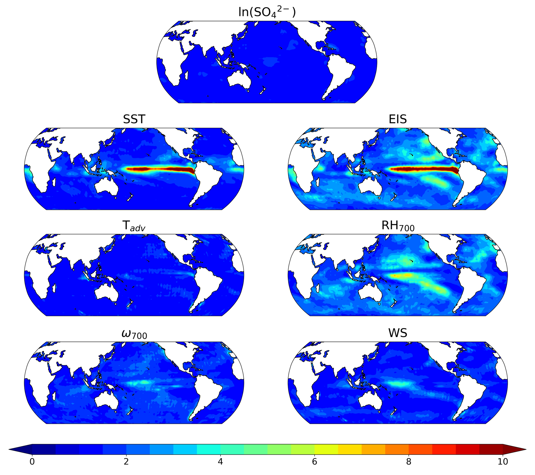
Figure A1 Variance inflation factors (VIFs) for each environmental factor Y_i in CCF analysis, calculated as ${\mathrm{VIF}}_i=\mathrm{1}/(\mathrm{1}-R_i^{\mathrm{2}})$, where $R_i^{\mathrm{2}}$ represents the total variance in Y_i explained by the remaining environmental predictors. The environmental predictors include natural logarithmic sulfate mass concentration (ln(${{\mathrm{SO}}_{\mathrm{4}}}^{\mathrm{2}-})$), sea surface temperature (SST), estimated inversion strength (EIS), horizontal surface temperature advection (T_adv), relative humidity at 700 hPa (RH₇₀₀), vertical velocity at 700 hPa (ω₇₀₀), and near-surface wind speed (WS).

A2 MERRA-2 reanalysis

We also use meteorological fields for cloud controlling factor analysis and sulfate aerosol mass concentrations (${{\mathrm{SO}}_{\mathrm{4}}}^{\mathrm{2}-}$) derived from the Modern-Era Retrospective analysis for Research and Applications, Version 2 (MERRA-2) reanalysis (Randles et al., 2017; Gelaro et al., 2017). MERRA-2 integrates observations with global model simulations to provide estimates of atmospheric conditions. Specifically for ${{\mathrm{SO}}_{\mathrm{4}}}^{\mathrm{2}-}$, it employs bias-corrected observations of total aerosol optical depth from the Moderate Resolution Imaging Spectroradiometer (MODIS; Platnick et al., 2015a, b) satellite data in conjunction with a comprehensive model addressing the emissions, removal processes, and chemistry of sulfate and its precursor gases. A notable feature of these data is that, while the total aerosol optical depth is observationally constrained, the distribution and vertical profiles of aerosol species are model-derived. In our analysis, we use ${{\mathrm{SO}}_{\mathrm{4}}}^{\mathrm{2}-}$ from 925 hPa instead of the surface level. This decision is based on the understanding that conditions near this altitude provide a more accurate reflection of CCN concentrations near the cloud base (Painemal et al., 2017). This pressure level is often closer to the actual height at which low-level clouds form, making it a more relevant indicator for assessing aerosol–cloud interactions.

A3 MODIS

We employ the aerosol index (AI) as an alternative proxy for aerosol concentration from MODIS on both the Aqua and Terra satellites (datasets MYD08_M and MOD08_M, respectively). These two are combined to enhance the robustness of our analysis. The AI is derived from the product of the Ångström exponent and the aerosol optical depth (AOD) at 550 nm. The Ångström exponent itself is derived from the wavelength dependency of the AOD, providing insight into the size distribution of aerosols (i.e., smaller Ångström exponent suggests larger particles). Notably, AI has demonstrated a more robust correlation with CCN compared to the use of AOD alone (Stier, 2016; Gryspeerdt et al., 2017; Hasekamp et al., 2019). However, it is important to note that since AI provides column-integrated quantities and does not account for the vertical profile, it may not accurately capture aerosol concentrations in low-level clouds, which are the focus of our study.

Figure A2 Same as Fig. A1 but for AI instead of ${{\mathrm{SO}}_{\mathrm{4}}}^{\mathrm{2}-}$.

We use cloud droplet number concentration (N_d) estimates from MODIS (Gryspeerdt et al., 2022a) and combine the data from the Aqua and Terra satellites. The retrievals at 3.7 µm, known to yield more accurate cloud droplet effective radius (r_e) measurements under inhomogeneous conditions, are employed (Zhang and Platnick, 2011). N_d measurements may be subject to biases under specific conditions, such as when the cloud droplet effective radius is sufficiently small, when the cloud visible optical thickness is low, or when three-dimensional radiative transfer effects impact the observed radiances. To enhance the accuracy and reliability of our N_d retrievals, we implement a rigorous sampling strategy (“BR17 sampling method” in Gryspeerdt et al., 2022a). This strategy introduced by Bennartz and Rausch (2017) demonstrates the highest correlation with aircraft data.

A4 GISTEMP

The global surface temperature observations used in our analysis are sourced from the GISS Surface Temperature Analysis (GISTEMP v4; Lenssen et al., 2019). We evaluate how well the models simulate the global-mean historical surface warming by the GOOD HIST index: the absolute difference in global-mean historical warming between CMIP6 models and GISTEMP data (Wang et al., 2021). The historical warming is defined as the averaged surface temperature in 1990–2014 minus that in 1880–1909. This suggests the models that are good at simulating historical warming have small GOOD HIST indices. For analysis, we select the 15 models with the lowest GOOD HIST indices (Table S1).

A5 CMIP6 data

Due to the unavailability of direct observational records for pre-industrial aerosol concentrations, we rely on the outputs from historical simulations with realistic emissions of greenhouse gases, aerosols, and aerosol precursor gases conducted by CMIP6 models to estimate changes in aerosol concentration (Δln (X), where X represents either ${{\mathrm{SO}}_{\mathrm{4}}}^{\mathrm{2}-}$ or AI). The pre-industrial (PI) period was defined as the years 1850 to 1899, and the present-day (PD) period was set from 1965 to 2014, each spanning 50 years to minimize the influence of interannual variability. Due to the limited availability of models for aerosol proxies, 13 models are used for $\mathrm{\Delta }\ln \left({{\mathrm{SO}}_{\mathrm{4}}}^{\mathrm{2}-}\right)$ and 9 models for Δln (AI), all models of which are among the 21 models that provide ERFaci_true (Table S1). It is important to note that, for the CMIP6 models, the emission concentrations of sulfur dioxide, a precursor to ${{\mathrm{SO}}_{\mathrm{4}}}^{\mathrm{2}-}$, are specified from the Community Emission Data Set (CEDS; Hoesly et al., 2018), and thus the projected changes in $\mathrm{\Delta }\ln \left({{\mathrm{SO}}_{\mathrm{4}}}^{\mathrm{2}-}\right)$ are highly consistent across models. The specified decadal trends in regional sulfate mass concentration in the models are also consistent with surface observations (Aas et al., 2019).

To evaluate our observationally constrained estimate of the ERFaci (ERFaci_obs), we employed 21 distinct models conducting single-forcing (aerosol-only) experiments (ERFaci_true). These models are from the Radiative Forcing Model Intercomparison Project (RFMIP; Pincus et al., 2016), specifically Tier 1 piClim-control and piClim-aer experiments with prescribed sea surface temperatures (SSTs) and sea ice derived from a climatology of pre-industrial conditions. These simulations are run for 30 years, incorporating realistic aerosol emissions in 1850 and 2014 to represent PI and PD conditions, respectively. This ensures an accurate estimation of the true baseline of ERFaci resulting solely from aerosol–cloud interactions. We use 30-year time periods for the PI and the PD scenario to evaluate ERFaci. Consequently, the ERFaci derived from these experiments is referred to as ERFaci_true.

A6 Cloud-controlling factor analysis

To improve our understanding of the cloud droplet number concentration and low cloud radiative effect in response to variations in aerosol concentration, we employed cloud controlling factor (CCF) analysis (Scott et al., 2020; Wall et al., 2022). This approach allows us to constrain the environmental factors influencing cloud droplets, low cloud properties, and their subsequent radiative impacts. The analysis considers a set of controlling factors that are known to be drivers of cloud droplets and low cloud behavior, which can be expressed as follows, respectively:

$$\begin{array}{}\text{(A2)}& {\displaystyle }{N}_{\mathrm{d}}{}^{\prime }\approx {\sum }_{i=\mathrm{1}}^{\mathrm{7}}{\displaystyle \frac{\partial N_{\mathrm{d}}}{\partial Y_i}}\times Y_i{}^{\prime }\text{(A3)}& {\displaystyle }\mathrm{CRE}\mathrm{\_}\mathrm{lcld}{}^{\prime }\approx {\sum }_{i=\mathrm{1}}^{\mathrm{7}}{\displaystyle \frac{\partial \mathrm{CRE}\mathrm{\_}\mathrm{lcld}}{\partial Y_i}}\times Y_i{}^{\prime },\end{array}$$

where N_d represents cloud droplet number concentration from MODIS, and CRE_lcld represents the non-obscured low-level cloud radiative effect from CERES. The factors (Y_i) from MERRA-2 reanalysis data included in our analysis are (1) sea surface temperature, (2) estimated inversion strength, (3) horizontal surface temperature advection, (4) relative humidity at 700 hPa, (5) vertical velocity at 700 hPa, and (6) near-surface wind speed. These parameters represent a combination of thermodynamic and dynamic influences that are critical in dictating low cloud formation and persistence (Scott et al., 2020). In addition to these standard meteorological variables, we introduce (7) aerosol concentration, as an additional controlling factor (Wall et al., 2022). Specifically, we consider either the natural logarithm of ${{\mathrm{SO}}_{\mathrm{4}}}^{\mathrm{2}-}$ at 925 hPa from the MERRA-2 reanalysis or the natural logarithm of the AI from MODIS.

For each grid point, we employ ordinary least-squares multilinear regression to model $N_{\mathrm{d}}^{\prime }$ or CRE_lcld^′ against anomalies in the seven cloud controlling factors. In this study, we focus specifically on the contribution of aerosol concentration variations to $N_{\mathrm{d}}^{\prime }$ or CRE_lcld^′, representing either activation rate ($\partial N_{\mathrm{d}}/\partial \ln \left(X\right)$) or susceptibility (∂CRE_lcld/∂ln (X)), while holding all other environmental conditions constant.

To assess potential multicollinearity among predictors, we calculated variance inflation factors (VIFs), as covariability among predictors can increase the uncertainty in regression coefficients (Figs. A1, A2). VIF values for each predictor remain below 5, except for SST and EIS over the equatorial Pacific, consistent with the VIF analysis by Scott et al. (2020). For aerosol proxies, such as ${{\mathrm{SO}}_{\mathrm{4}}}^{\mathrm{2}-}$ and AI, covariability with environmental factors is minimal and difficult to detect. This emphasizes the independence of aerosol concentrations from other environmental factors and supports that our ERFaci estimation is genuinely driven by aerosols.

A7 Estimating ERFaci using CMIP6 model outputs

A7.1 Estimating ERFaci_true

The ERFaci_true is calculated for PD minus PI conditions from aerosol-only, fixed-SST experiments as

$$\begin{array}{}\text{(A4)}& \mathrm{ERFaci}\mathrm{\_}\mathrm{true}=\mathrm{\Delta }\mathrm{CRE}\mathit{\_}\mathrm{lcld},\end{array}$$

where the low-level cloud radiative response (ΔCRE_lcld) is determined using cloud classification method introduced in Webb et al. (2006) and Soden and Vecchi (2011).

A7.2 Estimating ERFaci_SC17

This method partitions the low-level cloud radiative response observed in historical experiments into two components: one is a temperature-mediated component (i.e., cloud feedback) attributable to changes in the global-mean surface temperature and the other to aerosol–cloud interactions. The estimate of ERFaci is then obtained by subtracting the temperature-driven component from the low-level cloud radiative response, thus focusing solely on the impact of aerosol–cloud interactions.

$$\begin{array}{}\text{(A5)}& \mathrm{ERFaci}\mathrm{\_}\mathrm{SC}\mathrm{17}=\mathrm{\Delta }\mathrm{CRE}\mathrm{\_}\mathrm{lcld}-{\mathit{\alpha }}_{\mathrm{1}{\mathrm{pctCO}}_{\mathrm{2}}}\cdot \mathrm{\Delta }\stackrel{\mathrm{‾}}{T_s},\end{array}$$

where ${\mathit{\alpha }}_{\mathrm{1}{\mathrm{pctCO}}_{\mathrm{2}}}$ represents the low-level cloud feedback, derived from the 1 % CO₂ increase per year (1pctCO₂) scenario, which is calculated as the low-level cloud radiative response normalized by the corresponding global-mean surface warming. $\mathrm{\Delta }\stackrel{\mathrm{‾}}{T_s}$ denotes global mean temperature response to PD minus PI conditions. Because this method uses outputs from historical and 1 pctCO₂ simulations, it allows a much larger sample size of models to evaluate the two different versions of ERFaci_est.

A7.3 Estimating ERFaci_est

To estimate ERFaci_est, derived exclusively from CMIP6 model outputs calculated using Eqs. (1) and (2) from the main text, we use monthly anomalies spanning 2000 to 2014 in historical experiments for susceptibility calculation, after removing trends and climatological seasonality. We adhere to the same time frame for aerosol concentration changes as described in the main text. Additionally, given the challenges associated with deriving cloud-top N_d directly from CMIP6 model outputs, we adopt an alternative approach, which is the maximum N_d within a vertical atmospheric column (Saponaro et al., 2020; Jia and Quaas, 2023). Owing to the limited availability of models for CCF analysis, it is not explicitly employed in the estimation process of ERFaci_est. Instead, we assess the impact of including or excluding CCF analysis on ERFaci_obs to elucidate their influence on the estimation of ERFaci_est. The simplified version of Eqs. (1) and (2), which do not account for CCF analysis, are presented below:

$$\begin{array}{}\text{(A6)}& {\displaystyle }\begin{array}{rl}& \mathrm{ERFaci}\mathrm{\_}\mathrm{obs}\approx {\displaystyle \frac{\partial \mathrm{CRE}\mathrm{\_}\mathrm{lcld}}{\partial \ln \left(X\right)}}\times \mathrm{\Delta }\ln \left(X\right),\\ & \left(\text{without\hspace{0.17em} CCF\hspace{0.17em} analysis\hspace{0.17em} and\hspace{0.17em} activation\hspace{0.17em} rate}\right)\end{array}\text{(A7)}& {\displaystyle }\begin{array}{rl}& \mathrm{ERFaci}\mathrm{\_}\mathrm{obs}\approx \left({\displaystyle \frac{\partial \mathrm{CRE}\mathrm{\_}\mathrm{lcld}}{\partial \ln \left(N_{\mathrm{d}}\right)}}\times {\displaystyle \frac{\partial \ln \left(N_{\mathrm{d}}\right)}{\partial \ln \left(X\right)}}\right)\times \mathrm{\Delta }\ln \left(X\right)\\ & \text{(without\hspace{0.17em} CCF\hspace{0.17em} analysis\hspace{0.17em} but\hspace{0.17em} with\hspace{0.17em} activation\hspace{0.17em} rate).}\end{array}\end{array}$$

When applying these equations to estimate ERFaci_obs, we obtain best estimates of global-mean ERFaci_obs (without activation rate) of −1.64 for ${{\mathrm{SO}}_{\mathrm{4}}}^{\mathrm{2}-}$ and −1.85 for AI and global-mean ERFaci_obs (with activation rate) of −0.56 for ${{\mathrm{SO}}_{\mathrm{4}}}^{\mathrm{2}-}$ and −0.27 for AI. These values are 1.87, 2.01, 1.75, and 1.44 times larger, respectively, than those obtained when considering CCF analysis. In other words, by dividing model-driven ERFaci estimates by these factors, we can approximate its value under scenarios that include CCF analysis (ERFaci_est). These outcomes are employed in Figs. 3 and S3.

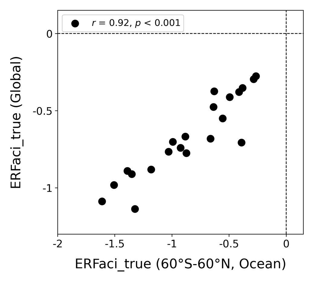
Figure A3 CMIP6 estimates of ERFaci_true, averaged for the domain region (60° S to 60° N over ocean), and globally averaged ERFaci_true values. Each black circle represents an individual model's estimate, with the correlation coefficient (r) and its associated p value (p) indicated in the upper left corner.

A8 Radiative kernel method

Originally developed by Soden et al. (2008) to facilitate the analysis of radiative feedbacks, “radiative kernels” describe the differential response of radiative fluxes to incremental changes in the radiative state variables (e.g., clouds, temperature, water vapor, albedo). In this study, we employed radiative kernel techniques derived from the HadGEM3-GA7.1 model (Smith et al., 2020b) for all CMIP6 model analysis, except for estimating ERFaci_est, as CCF analysis serves a similar role to the radiative kernel method in isolating the genuine cloud radiative response while minimizing interference from cloud masking effects.

A9 Extrapolating global-mean estimates from domain-mean estimates

Given that our observation data cover the domain extending from 60° S to 60° N over the ocean, it is necessary to extrapolate global-mean ERFaci values for comparison with the global-mean estimates reported in the IPCC Sixth Assessment Report and the WCRP. To bridge the gap between global and domain-specific averages we use 21 CMIP6 climate models in single-forcing experiments (ERFaci_true) to estimate a scalar, γ, representing the ratio of the multi-model mean of global-average ERFaci_true to domain-average ERFaci_true (Fig. A3). We ascertain γ's value at 0.86 with 0.92 correlation coefficient between models and a p value of less than 0.001, enabling us to adjust our domain-specific ERFaci estimates to better approximate the global mean. This extrapolation is performed using the following equation:

$$\begin{array}{}\text{(A8)}& \mathrm{ERFaci}\mathrm{\_}\mathrm{obs},\mathrm{global}=\mathit{\gamma }\times \mathrm{ERFaci}\mathrm{\_}\mathrm{obs},\mathrm{domain}.\end{array}$$

Additionally, following the approach of Wall et al. (2022), we conduct a sensitivity test for γ without relying on climate model results. In this alternative method, we assume that the albedo change associated with ERFaci is approximately uniform across the study domain and the entire globe. Under this assumption, γ is approximated as the ratio of global-mean insolation to domain-mean insolation, yielding a central estimate of 0.92. Notably, this value is highly consistent with our model-derived estimate of 0.86, supporting the robustness of our extrapolation approach. Given this consistency, we adopt γ=0.86 in this study.

We also apply this scalar multiplier to extrapolate the global mean activation rate, as variations in N_d in single-forcing (aerosol-only) experiments primarily result from changes in aerosol concentrations. This extrapolation remains consistent with the ratio of global mean ERFaci_obs calculated with and without accounting for activation rate, suggesting a global mean activation rate of 0.37 for ${{\mathrm{SO}}_{\mathrm{4}}}^{\mathrm{2}-}$ and 0.21 for AI.

Even though our study domain captures the primary anthropogenic aerosol sources, particularly near major industrial regions in Eurasia and North America, and our multi-model mean extrapolation inherently accounts for aerosol–cloud interactions outside our domain, recent studies have highlighted their significant influence in polar regions (e.g., Coopman et al., 2018). Aerosol-induced cloud property changes in the Arctic may be more efficient per unit aerosol mass than at mid-latitudes due to the greater susceptibility of Arctic clouds to aerosols. Incorporating these effects could lead to a more negative global-mean ERFaci estimate. The role of Arctic aerosol–cloud interactions warrants further investigation, and future research incorporating more comprehensive observational constraints would be valuable.

A10 Adjusting the IPCC's ERFaci estimate

We adjust the IPCC Sixth Assessment Report's estimate of ERFaci, which uses 2014 as the present-day reference year and 1750 as the pre-industrial reference year. The IPCC's initial global estimate for ERFaci between 2014 and 1750 is −1.0 ± 0.7 W m⁻². To make this pre-industrial reference period consistent with our analysis, we subtract the estimated ERFaci of −0.07 W m⁻² between 1850 and 1750 from the IPCC's value (Dentener et al., 2023). This adjustment yields an estimate based solely on observational evidence, with a 90 % CI of −0.93 ± 0.7 W m⁻² (Wall et al., 2022).

A11 Uncertainty

The uncertainty in ERFaci_obs, in the case where the activation rate is not considered, is attributed to uncertainties in the susceptibility, the regression coefficient for $\partial \mathrm{CRE}\mathrm{\_}\mathrm{lcld}/\partial \ln \left(X\right),$ and in the model estimates of Δln(X). Conversely, when considering the activation rate, the uncertainty in ERFaci_obs stems from uncertainties in the regression coefficients for $\partial \mathrm{CRE}\mathrm{\_}\mathrm{lcld}/\partial \ln \left(N_{\mathrm{d}}\right)$ and $\partial \ln \left(N_{\mathrm{d}}\right)/\partial \ln \left(X\right)$, as well as from uncertainties in the model predictions of Δln (X).

To quantify the uncertainty derived from regression coefficients, at each grid box a 90 % confidence interval of the susceptibility is given by

$$\begin{array}{}\text{(A9)}& {\displaystyle }\mathit{\delta }=t\sqrt{{\mathbf{C}}_{ii}}\sqrt{{\displaystyle \frac{N_{\mathrm{nom}}}{N_{\mathrm{eff}}}}}\left[\mathrm{\Delta }\ln \left(X\right)\right]\left(\text{without\hspace{0.17em} activation\hspace{0.17em} rate}\right),\text{(A10)}& {\displaystyle }\mathit{\delta }=t\sqrt{\mathrm{\Delta }{x}^T\mathbf{C}\mathrm{\Delta }x}\sqrt{{\displaystyle \frac{N_{\mathrm{nom}}}{N_{\mathrm{eff}}}}}\left[\mathrm{\Delta }\ln \left(X\right)\right]\left(\text{with\hspace{0.17em} activation\hspace{0.17em} rate}\right),\end{array}$$

where t is the critical value of Student's t test at the 95 % significance level with N_eff−7 degrees of freedom (von Storch and Zwiers, 1999); C is the variance–covariance matrix of regression coefficients, and hence C_ii represents the diagonal components of C; $N_{\mathrm{nom}}/N_{\mathrm{eff}}$ is the ratio of the nominal to effective number of monthly values of CRE_lcld^′; and Δx is the regression coefficient for $\partial \ln \left(N_{\mathrm{d}}\right)/\partial \ln \left(X\right)$. C is formulated as $\mathbf{C}={\widehat{\mathit{\sigma }}}^{\mathrm{2}}{\left(Z^{T}Z\right)}^{-\mathrm{1}}$, where Z is the data matrix with columns composed of detrended monthly anomalies. Specifically, these anomalies are of ln (X) in scenarios where the activation rate is not considered and of ln (N_d) in scenarios where the activation rate is included. The term ${\widehat{\mathit{\sigma }}}^{\mathrm{2}}$ denotes the mean of squared residuals of the regression model and we estimate $N_{\mathrm{nom}}/N_{\mathrm{eff}}$ as $(\mathrm{1}+r)/(\mathrm{1}-r)$, where r is the lag one autocorrelation of CRE_lcld^′. Square brackets indicate multi-model mean of a parameter.

Uncertainty for spatially averaged regression coefficients is calculated as

$$\begin{array}{}\text{(A11)}& {\mathrm{\Delta }}_{\mathrm{obs}}=\sqrt{{\displaystyle \frac{\sum _{k=\mathrm{1}}^{N_{\mathrm{nom}}^{\ast }}{\left({\mathit{\delta }}_k{w}_k\right)}^{\mathrm{2}}}{{\left(\sum _{k=\mathrm{1}}^{N_{\mathrm{nom}}^{\ast }}{w}_k\right)}^{\mathrm{2}}}}}\sqrt{{\displaystyle \frac{N_{\mathrm{nom}}^{\ast }}{N_{\mathrm{eff}}^{\ast }}}},\end{array}$$

where δ_k denotes the uncertainty of the kth grid box, and w_k is the cosine of the latitude. $N_{\mathrm{nom}}^{\ast }$ represents the nominal number of spatial degrees of freedom, while $N_{\mathrm{eff}}^{\ast }$ represents the effective number of spatial degrees of freedom. The ratio $N_{\mathrm{nom}}^{\ast }/N_{\mathrm{eff}}^{\ast }$ is determined through empirical orthogonal function (EOF) analysis applied to CRE_lcld^′ for all ocean grid boxes between 60° S and 60° N as outlined in Eq. (5) of Bretherton et al. (1999). Before conducting the EOF analysis, each grid of CRE_lcld^′ value is multiplied by $\sqrt{w_k}$ to mitigate dependencies on grid geometry (North et al., 1982). The derived value of Δ_obs quantifies the half-width of the 90 % CI for ERFaci_obs over our domain region, specifically reflecting the uncertainty associated with regression coefficients.

To estimate uncertainty derived from model predictions, we examine the entire range of aerosol concentration changes across each CMIP6 model, instead of estimating uncertainty within the 5th–95th percentile range, primarily due to the limited number of models available for our analysis: 13 models for Δln (SO₄) and 9 models for Δln (AI). This decision reflects a methodological adaptation to the limited model dataset, ensuring a comprehensive evaluation of model-derived uncertainty (Myers et al., 2023). We first calculate ERFaci_obs by multiplying Δln (X) from each of the models by the observationally derived susceptibility. The half-width of the CI, denoted as Δ_model, is derived by halving the difference between the maximum and minimum estimates of ERFaci_obs. The overall 90 % CI is determined by

$$\begin{array}{}\text{(A12)}& \mathrm{ERFaci}\mathrm{\_}\mathrm{obs},\mathrm{domain}\pm \sqrt{{\mathrm{\Delta }}_{\mathrm{obs}}^{\mathrm{2}}+{\mathrm{\Delta }}_{\mathrm{model}}^{\mathrm{2}}}.\end{array}$$

In our methodology, the scalar γ is used to extrapolate the global ERFaci_obs from our domain-specific ERFaci_obs estimates. This extrapolation introduces an additional component of uncertainty. Although both γ and the changes in aerosol concentration are obtained from CMIP6 model outputs, it is important to note that γ does not directly correlate with aerosol concentration changes across the models. Consequently, the uncertainty associated with γ is quantified using the root mean squared error (RMSE) between the domain-specific averaged ERFaci_true, multiplied by γ, and the global-mean ERFaci_true. The overall 90 % CI is determined by

$$\begin{array}{}\text{(A13)}& \mathrm{ERFaci}\mathrm{\_}\mathrm{obs},\mathrm{global}\pm \sqrt{{\left(\left[\mathit{\gamma }\right]{\mathrm{\Delta }}_{\mathrm{obs}}\right)}^{\mathrm{2}}+{\left(\left[\mathit{\gamma }\right]{\mathrm{\Delta }}_{\mathrm{model}}\right)}^{\mathrm{2}}+{\mathrm{\Delta }}_{\mathit{\gamma }}^{\mathrm{2}}}.\end{array}$$

The uncertainty in the activation rate is calculated in a similar manner, but it arises from the regression coefficient of $\partial \ln \left(N_{\mathrm{d}}\right)/\partial \ln \left(X\right)$ and the extrapolation of the global activation rate. The term δ is computed following Eq. (A9) but excluding [Δln (X)] and using ln (N_d)^′ in place of CRE_lcld^′. To estimate the uncertainty in spatially averaged regression coefficients for the activation rate, we employ Eq. (A11). Consequently, the overall 90 % CI for the global activation rate is given by

$$\begin{array}{}\text{(A14)}& \mathrm{activation}\mathrm{rate},\mathrm{global}\pm \sqrt{{\left(\left[\mathit{\gamma }\right]{\mathrm{\Delta }}_{\mathrm{obs}}\right)}^{\mathrm{2}}+{\mathrm{\Delta }}_{\mathit{\gamma }}^{\mathrm{2}}}.\end{array}$$