the Creative Commons Attribution 4.0 License.
the Creative Commons Attribution 4.0 License.
 | 11 Jul 2025
Global ground-based tropospheric ozone measurements: reference data and individual site trends (2000–2022) from the TOAR-II/HEGIFTOM project
Roeland Van Malderen
Anne M. Thompson
Debra E. Kollonige
Ryan M. Stauffer
Herman G. J. Smit
Eliane Maillard Barras
Corinne Vigouroux
Irina Petropavlovskikh
Thierry Leblanc
Valérie Thouret
Pawel Wolff
Peter Effertz
David W. Tarasick
Deniz Poyraz
Gérard Ancellet
Marie-Renée De Backer
Stéphanie Evan
Victoria Flood
Matthias M. Frey
James W. Hannigan
José L. Hernandez
Marco Iarlori
Bryan J. Johnson
Nicholas Jones
Rigel Kivi
Emmanuel Mahieu
Glen McConville
Katrin Müller
Tomoo Nagahama
Justus Notholt
Ankie Piters
Natalia Prats
Richard Querel
Dan Smale
Wolfgang Steinbrecht
Kimberly Strong
Ralf Sussmann
Tropospheric ozone trends from models and satellites are found to diverge. Ground-based (GB) observations are used to reference models and satellites, but GB data themselves might display station biases and discontinuities. Reprocessing with uniform procedures, the TOAR-II working group Harmonization and Evaluation of Ground-based Instruments for Free-Tropospheric Ozone Measurements (HEGIFTOM) homogenized public data from five networks: ozonesondes, In-service Aircraft for a Global Observing System (IAGOS) profiles, solar absorption Fourier transform infrared (FTIR) spectrometer measurements, lidar observations, and Dobson Umkehr data. Amounts and uncertainties for total tropospheric ozone (TrOC; surface to 300 hPa), as well as free- and lower-tropospheric ozone, are calculated for each network. We report trends (2000 to 2022) for these segments using quantile regression (QR) and multiple linear regression (MLR) for 55 datasets, including six multi-instrument stations. The findings are that (1) median TrOC trends computed with QR and MLR trends are essentially the same; (2) pole-to-pole, across all longitudes, TrOC trends fall within +3 to −3 ppbv per decade, equivalent to (−4 % to +8 %) per decade depending on site; (3) the greatest fractional increases occur over most tropical and subtropical sites, with decreases at northern high latitudes, but these patterns are not uniform; (4) post-COVID trends are smaller than pre-COVID trends for Northern Hemisphere mid-latitude sites. In summary, this analysis conducted in the frame of TOAR-II/HEGIFTOM shows that high-quality, multi-instrument, harmonized data over a wide range of ground sites provide clear standard references for TOAR-II models and evolving tropospheric ozone satellite products for 2000–2022.
- Article
(15587 KB) - Full-text XML
- Companion paper
-
Supplement
(2297 KB) - BibTeX
- EndNote


Tropospheric ozone, including ground-level ozone, plays a crucial role in atmospheric chemistry as a secondary pollutant formed by reactions between volatile organic compounds (VOCs) and nitrogen oxides (NOx) in the presence of sunlight (Vingarzan, 2004; Monks et al., 2015). In the stratosphere, ozone protects life from harmful ultraviolet rays. At ground level, ozone can harm human health and ecosystems, contributing to respiratory problems and crop damage (Lefohn et al., 2018; Mills et al., 2018). Additionally, tropospheric ozone is a potent greenhouse gas, contributing to climate change (IPCC, 2021). Thus, monitoring and controlling ozone levels is vital for environmental and public health.
Assessments of tropospheric ozone trends make use of several types of observations, among them surface ozone (Oltmans et al., 2013; Cooper et al., 2020), satellite estimates of full or partial ozone column content (Gaudel et al., 2018), aircraft (Gaudel et al., 2020), Fourier transform infrared tropospheric column (Vigouroux et al., 2015; Gaudel et al., 2018), and lidar (Granados-Muñoz and Leblanc, 2016; Ancellet et al., 2022) or ozonesonde profiles (Logan et al., 2012; Thompson et al., 2021, 2025; Van Malderen et al., 2021; Christiansen et al., 2017, 2022; Wang et al., 2022; Stauffer et al., 2024; Nilsen et al., 2024). In the first phase of the International Global Atmospheric Chemistry/Tropospheric Ozone Assessment Report (IGAC/TOAR), Gaudel et al. (2018) pointed out that five typical satellite products covering the 2005–2016 period differed greatly from one another, not only in magnitude but even in sign. A recent evaluation of six updated satellite products for 2004–2019 over the tropics (Gaudel et al., 2024), where satellite estimates tend to be most reliable (Thompson et al., 2021), also exhibited large divergence from one another. When compared to aircraft and ozonesonde profiles up to 270 hPa, some satellite comparisons for the years 2014–2019 showed correlations with R2 ∼ 0.3–0.6 (Gaudel et al., 2024). Recent harmonization efforts of 16 global tropospheric ozone satellite data records could only partially account for the observed discrepancies between the satellite datasets, with a reduction of about 10 %–40 % of the inter-product dispersion upon harmonization, depending on the products involved, and with strong spatiotemporal dependences (Keppens et al., 2025).
Chemistry–transport and coupled chemistry–climate models also vary greatly in tropospheric ozone due to uncertainties in anthropogenic emissions and/or different parameterizations for dynamical processes, e.g., treatments of boundary layer processes, convection, and stratosphere–troposphere exchange (e.g., Christiansen et al., 2022). Accordingly, both model output and satellite products, global in coverage, use networks of ground-based (GB) observations for evaluation (e.g., recently in Gong et al., 2025, and Jones et al., 2025, for model evaluation and in Arosio et al., 2024; Pennington et al., 2024; Dufour et al., 2025; Keppens et al., 2025; and Maratt Satheesan et al., 2025 for satellite validation). GB networks, with stations operating at fixed sites using well-characterized instruments, typically calibrated with world reference standards, provide suitable time series at more than 100 sites. However, GB data themselves display station biases and discontinuities, especially when instruments or processing methods change. Within the umbrella of the Network for the Detection of Atmospheric Composition Change (NDACC; De Mazière et al., 2018), working groups for several spectral ozone instruments have standardized data processing. The IGAC/TOAR-II project recognized that these spectrometric data as well as soundings and aircraft profiles provide the free-tropospheric (FT) information that is essential for model calculations of radiative forcing. The TOAR-II working group Harmonization and Evaluation of Ground-based Instruments for Free-Tropospheric Ozone Measurements (HEGIFTOM) was formed in 2021 to homogenize and archive publicly available data from five network types: ozonesondes, In-service Aircraft for a Global Observing System (IAGOS) profiles, Fourier transform infrared spectrometer (FTIR), lidar, and Dobson Umkehr. In addition to uniform procedures for data reprocessing within each network, uncertainty estimates and quality flags were provided. HEGIFTOM data can be downloaded via https://hegiftom.meteo.be/datasets (last access: 8 April 2025).
This article first gives details of harmonization methods for the five instrument types (Sect. 2) as well as three analysis methods for ozone trends over the 2000 to 2022 period (Sect. 3). Results begin with a climatology for a nominal total tropospheric ozone column amount (surface to 300 hPa or TrOC) (Sect. 4.1). Observational evidence for seasonal shifts over the 23-year period is also illustrated with a summary examination of COVID-19 impacts on the mean 2000–2022 TrOC. This is followed by two general sets of trend results (Sect. 4.2). Most of the focus is on TrOC trends for which all five GB methods have some information. Trends for a FT ozone column (between 700 and 300 hPa) and a lower-tropospheric (LT) column (surface to 700 hPa), which use only profiles from ozonesondes, aircraft, and lidar, are also presented. The individual site trends for TrOC are computed with two statistical approaches, quantile regression (QR) and multiple linear regression (MLR). In all cases trend results are tabulated and displayed in TOAR-II-preferred ppbv per decade units (Chang et al., 2023), but percent (%) per decade units are also used to allow meaningful comparisons across all sites. In Sect. 4.3, seasonal characteristics of trends are compared across instruments at six multi-sensor sites and across stations within densely sampled sub-regions in Europe and parts of North America. Comparisons of TrOC trends made with QR and MLR across multiple instruments at a single site give insights into some differences in trends derived from the sensors as do drifts among collocated instruments relative to one another. Section 5 is a summary with prospects for a merging of selected individual site data and further reprocessing, harmonization, and expansion of data in the HEGIFTOM archive.
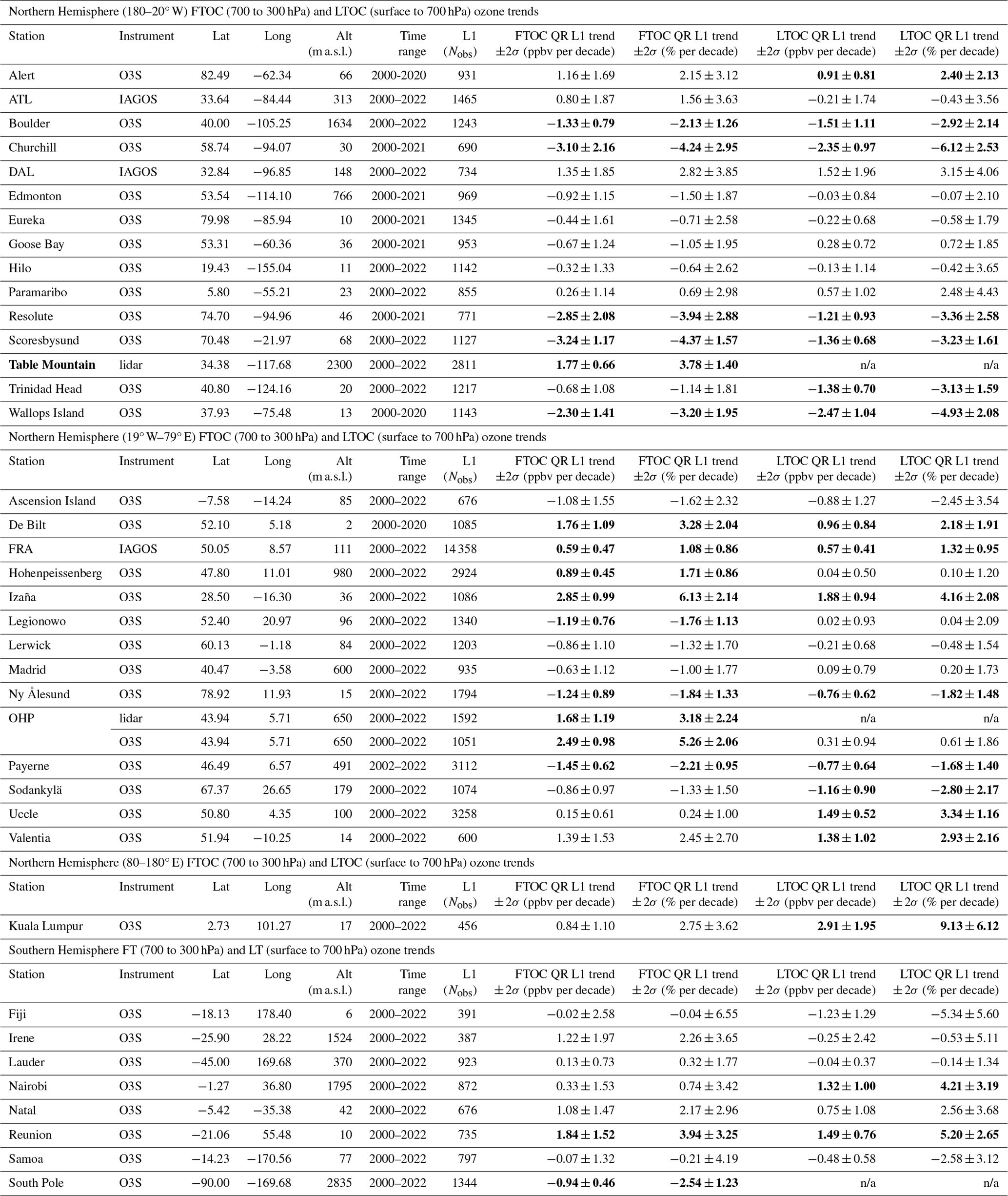
The five GB instruments considered here provide ozone profiles with high (ozonesondes, IAGOS, lidar) or low (Umkehr, FTIR) vertical resolution. After homogenization, different tropospheric ozone columns are calculated or retrieved from the profile measurements and are available at the HEGIFTOM archive, https://hegiftom.meteo.be/datasets/tropospheric-ozone-columns-trocs (last access: 8 April 2025). The total number of sites for which those tropospheric ozone columns can be downloaded is 356, made up of 280 IAGOS airports, as well as 43 ozonesonde, 25 FTIR, 6 Dobson/Umkehr, and 2 lidar sites. A map and table showing all the sites or airports that have had data available since 2000 are provided in Fig. S1 and Table S1 in the Supplement, respectively. In this paper, to calculate trends for the 2000–2022 period, we only retained time series starting in 2000–2002 and ending in 2019 or later, as recommended by the TOAR-II statistical guidelines (Chang et al., 2023). We also required that time series have at least 120 monthly values available (about half of the maximum coverage), essentially the lower limit for computing both reliable trends and uncertainties from monthly mean time series with the three used trend estimation tools. The final selection of stations used in our trend analyses is presented in Table 1 and Fig. 1. In Fig. 1, five types of network instruments are included with color coding: ozonesondes (34 sites, black circles), IAGOS aircraft profiles (three airports, magenta stars), FTIR (10 sites, cyan squares), Umkehr from Dobson spectrometers (six sites, red circles), and lidar (two sites, gray squares). A total of 55 datasets (Table 1) are used with six sites having more than one instrument type in operation as shown in Table 1 and Fig. 2. In this study, we focus on tropospheric ozone columns with different metrics that were calculated and made available in the HEGIFTOM archive. Of particular interest is the total tropospheric ozone column extending from the surface up to about 300 hPa; this is the only common metric for all five instruments. The 300 hPa lower pressure limit has been chosen because lower pressure levels are globally not always reached with the IAGOS aircraft. Umkehr and FTIR usually have only a maximum of 1 degree of freedom in the whole troposphere, so the division in smaller partial columns would not provide independent information. For the other three techniques, we also consider free-tropospheric ozone column (FTOC), defined here between 700 and 300 hPa, and lower-tropospheric ozone column (LTOC), between the surface and 700 hPa. All those (partial) tropospheric ozone columns are provided in ppb (as column-averaged integrated ozone mixing ratios) and DU, as well as with different temporal resolutions: all measurements (L1), daily means (L2), and monthly means (L3). In the following subsection, particulars of each dataset type and its harmonization are described. A more detailed description of the tropospheric ozone measurements with those different techniques is available in, e.g., Tarasick et al. (2019).
Table 1Sample (55 sites total) stations and instruments. Stations used in TrOC (surface to 300 hPa column) trend calculations, with instrument type, location, altitude, sample time range, and all-sample number of observations (L1) and monthly means (L3), with corresponding trends in ppbv per decade ± 2σ. Bold trends have p<0.05.
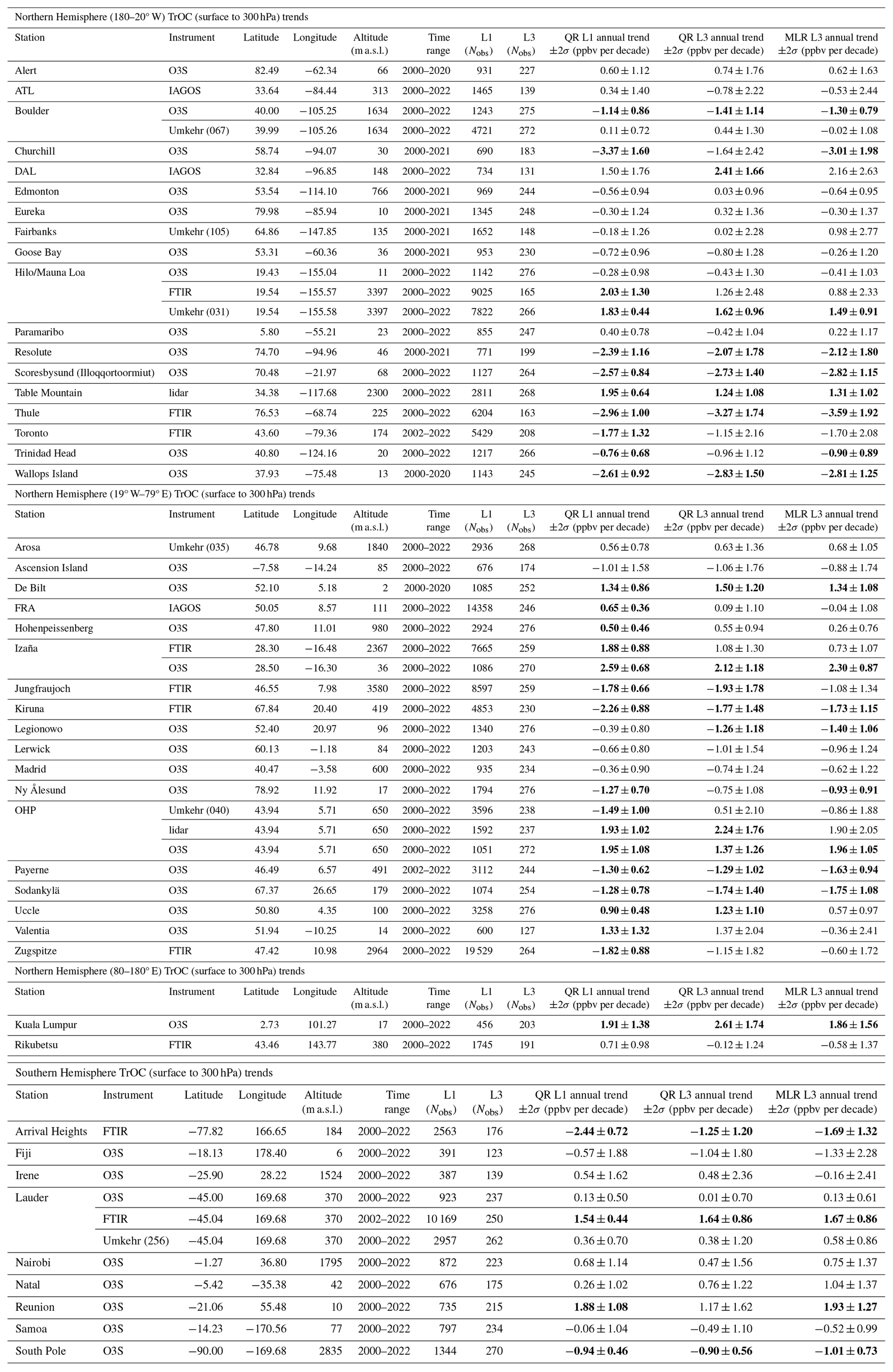
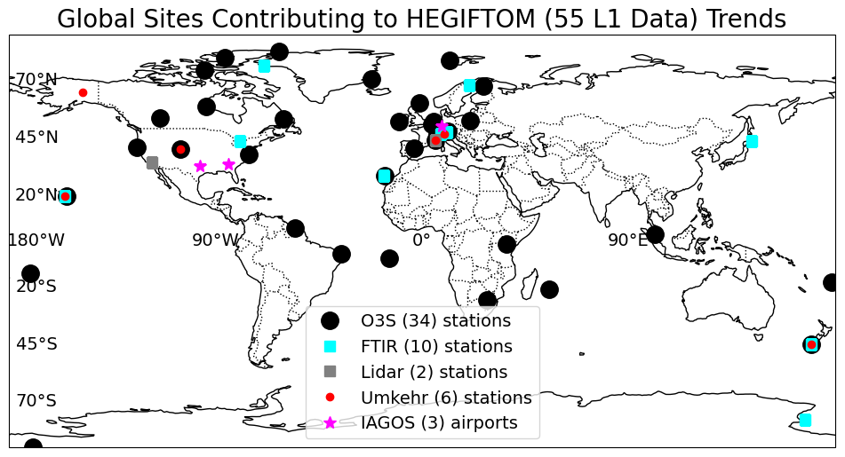
Figure 1Partial map of sites for which ozone data have been homogenized and TrOC are available at the HEGIFTOM archive: https://hegiftom.meteo.be/datasets/tropospheric-ozone-columns-trocs (last access: 8 April 2025). Five types of instruments are archived, color-coded as in key. Details on instrumentation, sample characteristics, and locations are presented in Table 1. Colors are superimposed at sites with data from more than one instrument (Table 1). Map shows 55 sites for which trends are computed according to the criteria: (1) all datasets must start within 2000–2002 and end within 2019–2022 (see TOAR-II statistical guidelines, Chang et al., 2023) and (2) more than 120 monthly mean values.
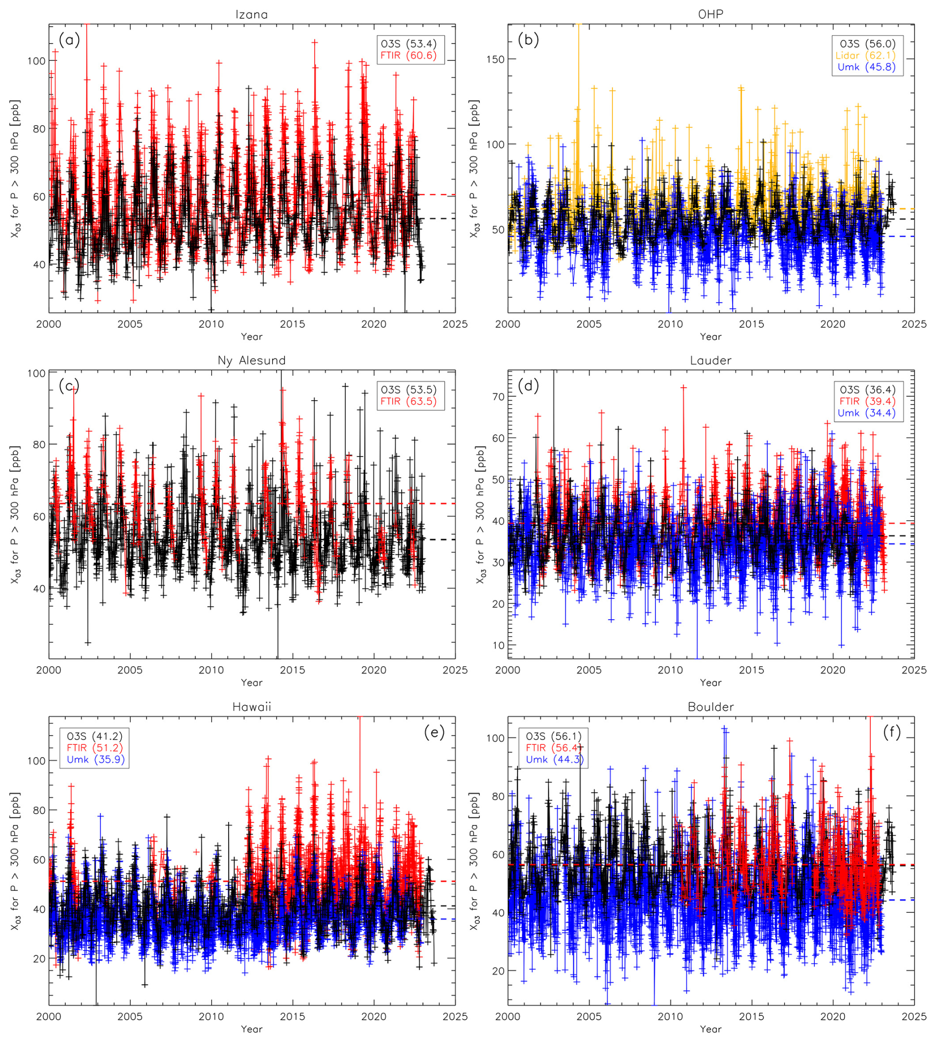
Figure 2TrOC daily mean (L2) time series, 2000–2022, for collocated instruments as archived in the HEGIFTOM database. Dashed lines are the long-term mean values over a 23-year period. (a) Izaña; (b) Observatoire de Haute-Provence (OHP); (c) Ny Ålesund; (d) Lauder; (e) Mauna Loa and Hilo, Hawaii; (f) Boulder. Note that the FTIR time series in Boulder and Ny Ålesund do not fulfill our criteria used for trend detection here. Measurements with time gaps of more than 4 months are not connected with lines.
2.1 Ozonesondes
The ozonesonde is a small and lightweight instrument that measures atmospheric ozone concentrations by pumping and bubbling air in differing concentrations of potassium iodide (KI) solutions in electrochemical concentration cells (ECCs). Known as the ECC sonde, this type is used in the HEGIFTOM analyses (except for Hohenpeissenberg, which uses the Brewer–Mast type). Coupled with a radiosonde during a weather balloon flight, the ECC ozonesonde provides vertical ozone profiles up to about 30–35 km altitude with a stated precision of 3 %–5 % and an uncertainty of about 5 %–10 % for both the troposphere and stratosphere (Smit et al., 2021). Since 1996 a series of laboratory ECC sonde evaluations have been conducted in the World Calibration Centre for Ozone Sondes (WCCOS) in Jülich, Germany, where a standard ozone photometer (OPM) is employed as the absolute reference in the so-called Jülich ozonesonde intercomparison experiments (JOSIE; Smit et al., 2007). The same OPM was flown on a single gondola with 18 sondes in a field experiment (BESOS) in 2004 (Deshler et al., 2008). The outcome of BESOS and the early JOSIE was the formation of an expert sonde team activity, Assessment of Standard Operating Procedures for Ozonesondes (ASOPOS), that codified sonde preparation handling and data processing in a WMO/GAW report (Report 201 by Smit and the ASOPOS Panel, 2014). Following the GAW Report 201, the most recent JOSIE took place in 2017 (Thompson et al., 2019), which, together with the activity described in the next paragraph, led to a second ASOPOS WMO/GAW report (Report 268, Smit et al., 2021).
Major contributors to uncertainties in ozone trends are discontinuities and biases in the long-term records of ozonesonde sites. Therefore, an Ozonesonde Data Quality Assessment (O3S-DQA) activity was initiated in 2011 (Smit and O3S-DQA Panel, 2012) to homogenize temporal and spatial ozonesonde data records under the framework of the SI2N initiative on Past Changes in the Vertical Distribution of Ozone (Hassler et al., 2014). The O3S-DQA homogenization design serves three major purposes: (i) removing all known inhomogeneities or biases due to changes in equipment, operating procedures, or processing; (ii) ensuring consistency of records across the ozonesonde network by providing and applying standard guidelines for data (re)processing steps (Smit and O3S-DQA Panel, 2012; appendices C and D in Smit et al., 2021); and (iii) providing an uncertainty estimate for each ozone partial pressure measurement in the profile. The O3S-DQA guidelines for data processing, standards, and uncertainty estimation are now the current recommendations in WMO/GAW Report 268 (Smit et al., 2021). About two-thirds of the current regularly operating stations have reprocessed and homogenized their data and made them publicly available (Tarasick et al., 2016; Van Malderen et al., 2016; Thompson et al., 2017; Witte et al., 2017, 2018, 2019; Sterling et al., 2018; Ancellet et al., 2022; Zeng et al., 2024; Nilsen et al., 2024). Only those homogenized ozonesonde data archived in the HEGIFTOM database are used in the analyses below.
The () ozone sensor response time (∼ 30 s) gives the ozonesonde a vertical resolution of about 150 m for a typical balloon ascent rate, so there are about 100 independent data points in the troposphere. To calculate tropospheric ozone columns in DU and ppb, the different ozone concentrations in the respective units at the pressure levels within a tropospheric column are integrated and only for the case of retrieving the column-averaged tropospheric ozone mixing ratio divided by the extent of the column. The uncertainties of tropospheric ozone columns are obtained by the squared sum of the individual uncertainties of the ozone concentration measurements. The monthly mean tropospheric ozone columns (L3) are only calculated if at least two ozonesonde measurements are available within that month.
2.2 IAGOS
The In-service Aircraft for a Global Observing System (IAGOS) is a European Research Infrastructure for global observations of atmospheric composition from commercial aircraft. IAGOS combines the expertise of scientific institutions with the infrastructure of civil aviation in order to provide essential data on climate change and air quality at a global scale (http://www.iagos.org, last access: 25 October 2024; Petzold et al., 2015; Thouret et al., 2022). IAGOS, previously named MOZAIC (Marenco et al., 1998), has recorded ozone mixing ratios from takeoff to landing since August 1994 over more than 70 000 flights, thus providing vertical profiles from near the ground to up to 12 km altitude over hundreds of airports worldwide. Note that only a few airports include sufficient time-series length and measurement frequency to allow statistically significant long-term trend analysis, as presented here. The remaining datasets require merging to form clusters for specific regions (e.g., in the tropical area as presented in Tsivlidou et al., 2023). The MOZAIC/IAGOS ozone data set complements other networks of in situ ozone measurements by providing data in regions poorly sampled or not at all as well as offering high-frequency measurements over some hubs of participating airlines, e.g., Frankfurt (FRA). Therefore, the MOZAIC/IAGOS record has been widely used for climatological and trends analysis (e.g., Petetin et al., 2016; Cohen et al., 2018; Gaudel et al., 2020; Wang et al., 2022; Gaudel et al., 2024) as well as model evaluations (e.g., Wagner et al., 2021; Eskes et al., 2024).
The ozone analyzer that has been installed on board each of the 5 to 10 commercial aircraft in operation since 1994 is a manufactured dual-beam UV absorption instrument modified to meet the aeronautical constraints including autonomous long-term operations. The response time is 4 sec as detailed in Thouret et al. (1998); the characteristics of ozone measurements performed on board the five MOZAIC aircraft include a detection limit 2 ppbv and uncertainties for individual (4 s) measurements ± [2 ppbv + 2 %]. The instrument technique, the standard operating procedures, and the pre- and post-flight calibrations have remained unchanged from MOZAIC to IAGOS (Nédélec et al., 2015). Ensuring the high quality of the ozone dataset is one of the main objectives of IAGOS. Indeed, systematic comparisons of different instruments on the same route or profile are continuously performed to control the internal consistency of the set of instruments and the long-term stability of the IAGOS ozone data set. This is confirmed, documented, and synthesized in Blot et al. (2021). More recently, an intercomparison exercise between the IAGOS instrument and the world standard ozone photometer for ozonesondes was conducted in the environmental simulation chamber of the World Calibration Center of Ozone Sondes (WCCOS) at Jülich (Germany), showing a good agreement of the two techniques within better than 2 %–5 % throughout the depth of the troposphere (Smit et al., 2025).
To calculate tropospheric ozone columns for the analysis presented here, vertical profiles of ozone mixing ratios measured by IAGOS are processed as follows. For individual profiles (L1 data), the average tropospheric ozone concentration (in ppbv) within a partial column is calculated by averaging the individual ozone mixing ratio measurements within the column. The total tropospheric ozone (in DU) for the partial column is determined by integrating the measured ozone mixing ratios with respect to height (in meters), weighted by the simultaneously measured air density profile. The uncertainties of both the average ozone concentration (in ppbv) and the total ozone (in DU) are derived from the uncertainties of individual measurements ± [2 ppbv + 2 %] using the same respective formulas. Daily means (L2 data) are computed as the arithmetic mean of the corresponding L1 data samples, while monthly means (L3 data) are obtained as the arithmetic mean of the L2 data samples (daily means). No minimum sample size is required for calculating daily or monthly means. The total uncertainties of daily means are calculated as the square root of the sum of the squares of the L1 uncertainties. Similarly, the total uncertainties of monthly means are computed as the square root of the sum of the squares of the L2 uncertainties.
2.3 FTIR
The FTIR (Fourier transform infrared) technique provides remote sensing solar absorption measurements of many trace gases in the atmosphere at more than 20 stations that are affiliated with NDACC. Within the NDACC Infrared Working Group (IRWG, https://www2.acom.ucar.edu/irwg, last access: 25 October 2024), considerable effort is made to harmonize target gas measurements and retrievals. First, the instruments, which are high-spectral-resolution spectrometers, are all from the same manufacturer (mainly Bruker 120/5HR or 120/5M). Requirements on spectral noise and verification of the correct alignment of the spectrometer need to be fulfilled before the station affiliation with NDACC is accepted. Then, only two different retrieval codes that provide results in close agreement (Hase et al., 2004) are used within the network, SFIT4 or PROFITT. These codes are based on optimal estimation from Rodgers (2000), which requires a priori profile information of atmospheric species and pressure/temperature profiles. The basic principle of FTIR retrievals is that the spectral line shapes provide some information on the target gas vertical distribution thanks to the pressure and temperature line broadening effect. Finally, the retrieval strategies for each NDACC target species are harmonized by providing guidelines to ensure that the same parameters are used within the network: among them are the spectroscopic database; the spectral windows with target signatures; and the pressure, temperature, and gas a priori profile information.
For ozone, the harmonization followed is described in Vigouroux et al. (2015), who use HITRAN 2008 for the spectroscopic parameters. An update of the retrievals is in progress within the network that will prescribe the use of HITRAN 2020. This will have an effect of reducing by 2 %–3 % the observed biases between the ozone UV and IR spectral ranges (Björklund et al., 2024; Gordon et al., 2022). Unfortunately, not all NDACC stations have yet adopted this new procedure.
As described in Vigouroux et al. (2015), FTIR ozone measurements can provide low-vertical resolution profiles with 4–5 DOFS (degrees of freedom for signal), distributed roughly as one independent vertical layer in the troposphere and three in the stratosphere, as given by the averaging kernels associated with the retrievals. Some FTIR stations have monitored ozone since the mid-1990s, and this technique has been commonly used in the past for ozone trend studies (Vigouroux et al., 2008, 2015; García et al., 2012; Harris et al., 2015; Gaudel et al., 2018; Steinbrecht et al., 2017; SPARC/IO3C/GAW, 2019; Godin-Beekmann et al., 2022; WMO, 2022). The FTIR tropospheric ozone columns have been used for IASI long-term validation in Boynard et al. (2018).
For the present HEGIFTOM work, tropospheric ozone columns have been provided for TrOC, as well as their random and systematic uncertainties calculated from the Rodgers formalism (Vigouroux et al., 2008; García et al., 2012), which are approximately 10 % and 3 %, respectively. Note that the dominant random uncertainty source for tropospheric ozone is the smoothing error, with the random noise uncertainty being much lower (about 2 %). No lower limit of available observations has been set for calculating daily or monthly means.
2.4 Dobson Umkehr
Umkehr is the observational method developed by Götz et al. (1934) to detect ozone change in several atmospheric layers including the troposphere and lower, middle, and upper stratosphere. The most recent version of the retrieval algorithm is described in Petropavlovskikh et al. (2005) and is operationally used to derive ozone profiles from zenith sky observations at several NOAA-GML and WMO-GAW Dobson stations (see station information at https://www.woudc.org, last access: 12 June 2024). The operational Umkehr algorithm is based on the Bass and Paur (BP) ozone cross-section (Bass and Paur, 1985). However, the impact of modifying cross-section spectral datasets (including temperature sensitivity analyses) was found to be negligible (less than 2 %, i.e., Petropavlovskikh et al., 2011). Several Umkehr records were used in the TOAR climate paper for tropospheric trend detection (Gaudel et al., 2018). The long-term records (including the longest continuing record collected since 1958 at Arosa station) were further homogenized to remove step changes in the data caused by instrumental artifacts and to ensure stability of the records for trend analyses (Petropavlovskikh et al., 2022; Maillard Barras et al., 2022). Assessment of Umkehr biases (±5 % in stratosphere and up to 10 % in the troposphere) and drifts relative to alternative observing systems (i.e., ozonesonde, satellite, models) were also addressed in Petropavlovskikh et al. (2022). Umkehr records are typically used to assess ozone trends in the stratosphere (SPARC/IO3C/GAW, 2019; Godin-Beekmann et al., 2022).
For HEGIFTOM we use ozone profile data that are gridded on the finely resolved pressure layers (Balis et al., 2024). However, because the Umkehr method has limited vertically resolved information in the troposphere, as identified by its relatively wide averaging kernel (Björklund et al., 2024), only one product is recommended for this paper: partial column below 300 hPa. Note that the Umkehr ozone profile is derived in Dobson units (1 DU = 2.69 × 1016 cm−2); mixing ratios used here are converted from DU partial columns. For the daily mean values (L2), no lower limit of available observations is imposed, so the daily mean data will contain either the mean of the AM and PM data (if available) or AM or PM data. For L3 (monthly mean) data, a minimum of two L2 measurements in each month is required.
2.5 Lidar
The ozone differential absorption lidar (DIAL) technique (using the absorption and backscatter of laser light by atmospheric molecules) has been used for about 4 decades and was first described in Mégie et al. (1977). Long-term routine measurements from two NDACC ozone DIAL instruments are used in the present study, namely from the Jet Propulsion Laboratory (JPL) Table Mountain Facility (TMF), California, tropospheric ozone lidar (TMTOL; McDermid et al., 2002) and from the Observatoire de Haute-Provence (OHP), France, tropospheric ozone lidar (LiO3Tr; Ancellet et al., 1989). TMTOL uses a combination of three DIAL pairs at 289/299 nm, one pair at 266/289 nm, and one pair at 299/355 nm, ensuring 3 h averaged nighttime ozone profiles with a total uncertainty comprised between 2 % and 15 % over the altitude range 0–21 km a.g.l. and with an effective vertical resolution ranging between 30 m and 2 km. The entire dataset (1999–present, 2500+ profiles) has been re-analyzed and homogenized using the NDACC-standardized uncertainty and vertical resolution recommendations described in Leblanc et al. (2016a, b). The TMTOL measurements have been compared and validated on many occasions using ozonesonde and collocated lidars, most recently during the Southern California Ozone Observation Project (SCOOP) campaign (Leblanc et al., 2018).
The OHP LiO3Tr uses a combination of two DIAL pairs at 299/316 nm, providing 2 h averaged after sunset ozone profiles with a total uncertainty comprised between 5 % and 15 % over the altitude range 2–13 km a.g.l. and with an effective vertical resolution ranging between 200 m and 1.5 km. Most of the dataset (1990–present) has been re-analyzed, homogenized, and validated against collocated ozonesondes (Ancellet et al., 2022). TrOC was computed for both TMF and OHP lidars according to the agreed HEGIFTOM working group definitions. The lidar ozone number density measurement is integrated to partial column (in DU) and converted to the column-averaged tropospheric ozone mixing ratio (ppb) using pressure/temperature (density) outputs from the MERRA-2 model interpolated at the TMF and OHP sites. Lidar measurements do not always cover the entire troposphere. Occasionally, cloud layers contaminate the measurements. In those cases, ozone cannot be retrieved inside the cloud layers, and outputs from the MERRA-2 model are used to avoid data gaps and ensure consistent TrOC datasets over the full period of trend derivation. MERRA-2 ozone outputs are also used at the bottom and top of the lidar profiles if the profiles do not extend far enough (downward or upward) to cover the entire column matching the HEGIFTOM TrOC definitions. Overall, the free-tropospheric partial columns referred to as “300–700 hPa” contain the best information content from lidar and should be considered the most reliable component of lidar TrOC in the rest of this study.
3.1 Trend calculations
Three trend methods have been employed in the HEGIFTOM analyses. TOAR-II recommends (Chang et al., 2023) using quantile regression (QR) because it is robust to intermittent data gaps and it yields trends among various segments of the ozone distributions, e.g., the lowest 5th percentile, representing low-ozone conditions typical of regions with minimum human influence; the median 50th percentile; and the 95th percentile, or most polluted samples. QR is favored by many tropospheric ozone researchers because sampling variability at many monitoring sites is highly varied (Gaudel et al., 2020; Chang et al., 2021; Wang et al., 2022; Chang et al., 2023). Multiple linear regression (MLR) analysis of monthly averaged ozone amounts has long been the workhorse of the stratospheric ozone community (Steinbrecht et al., 2017; SPARC/IO3C/GAW, 2019; Godin-Beekman et al., 2022; WMO, 2022). It is applied to globally gridded satellite data; various oscillations – e.g., seasonal and annual cycles, the QBO, and solar cycles – are routinely included in model fits to the data. Dynamical linear modeling (DLM) is applied to a subset of our sample for further analysis of the collocated and nearby sites.
3.1.1 Quantile regression (QR)
Quantile regression is a percentile-based method (Koenker, 2005); thus, the heterogeneous distributional changes in the trends can be estimated. In this study this method is applied to the median change in the trends, which is equivalent to the least absolute deviation estimator (i.e., aiming to minimize mean absolute deviation for residuals; Chang et al., 2021). Compared to the least-squares criterion, the median-based approach is more robust when extreme values or outliers are present. Median trends are estimated based on the following multivariate linear model:
where t is the time step (all measurements, L1, or months, L3), tM is the month, harmonic functions are used to represent the seasonality, a0 is the intercept, b is the trend value, c is the regression coefficient for ENSO (Multivariate ENSO Index, MEI, v2; https://www.psl.noaa.gov/enso/mei/, last access: 28 August 2024), and ∈(t) represents the residuals. The MEI ENSO term is only applied for stations within 15° latitude of the Equator. ENSO impacts to ozone are expected to be minimal outside of the tropics. Autocorrelation is accounted for by using the moving-block-bootstrap algorithm, and the implementation details are provided in the TOAR statistical guidelines (Chang et al., 2023).
3.1.2 Multiple linear regression (MLR)
We compare the QR results to annual and monthly tropospheric ozone trends derived from the monthly L3 data with a multiple linear regression (MLR) model. MLR has long been the standard for computing ozone trends from satellite- and ground-based datasets, including Nimbus 7 TOMS (Stolarski et al., 1991), OMI/MLS (Ziemke et al., 2019), merged satellite data (Szeląg et al., 2020; Godin-Beekmann et al., 2022), ozonesondes, lidar, and FTIR (e.g., Steinbrecht et al., 2017; Thompson et al., 2021; Godin-Beekmann et al., 2022; Stauffer et al., 2024). The MLR model can include proxies known to affect ozone concentrations such as ENSO, the QBO, and the solar cycle, among others. Here, we use a simplified version of the MLR model implemented in Thompson et al. (2021) and Stauffer et al. (2024) and include only the ENSO term within 15° of the Equator (see Eq. 1). In Eq. (1), t is now the month and equals tM, because the MLR is applied on L3 data only. The 95 % confidence intervals for the MLR model terms are determined with a moving-block-bootstrap technique with 1000 resamples to account for autocorrelation in the time series as was done in Thompson et al. (2021) and Stauffer et al. (2024).
3.1.3 Dynamical linear modeling (DLM)
Dynamical linear modeling (DLM) allows for the determination of a nonlinear time-varying trend from a monthly mean time series. This is a Bayesian approach regression which fits the data time series for a nonlinear time-varying trend and seasonal and annual modes. Regression coefficients from explanatory variables have not been considered here. The trend is allowed to smoothly vary in time, and its degree of nonlinearity is inferred from the data. We use the code implemented in Python by Alsing et al. (2019) from the formalism introduced by Laine et al. (2014). The model used allows for a variability of the sinusoidal seasonal modes and includes the autoregressive (AR1) correlation process with variance and correlation coefficient as free parameters in the regression. The estimation of the posterior uncertainty distribution is performed with the Markov chain Monte Carlo (MCMC) method and considers the uncertainties on the seasonal cycle, on the autoregressive correlation, and on the nonlinearity of the trend. DLM trend estimations show good agreement with MLR trend estimations on stratospheric ozone profiles, ozone total, and partial columns measured by ground-based instruments (Maillard Barras et al., 2022; Steinbrecht et al., 2025) and satellites (Ball et al., 2017; WMO, 2022).
4.1 Tropospheric ozone column distribution
4.1.1 Tropospheric ozone column comparisons between different techniques
Table 1 shows that there are six sites with more than one instrument type: Izaña (2 instruments), OHP (3), Ny Ålesund (2), Lauder (3), Hawaii (3), and Boulder (3). These typically feature ozonesondes and one or more spectrometers. We refer to these as “collocated” sites. In Fig. 2 the consistency of TrOC measurements from the multiple sets of instruments can be compared by looking at their time series of daily values and comparing the means of each instrument (dashed lines in Fig. 2). Some systematic differences between the TrOC mean values among the techniques at the collocated sites are observed: a positive and negative bias of FTIR and Umkehr, respectively, with respect to ozonesondes. The same observation can be made when looking at the time series of daily values within a region or “nearby” sites in Fig. 3, as illustrated for the eastern US (Fig. 3a), Japan and southeast Asia (several instrument types, Fig. 3b), and among instrument types within Europe (Fig. 3c–f).
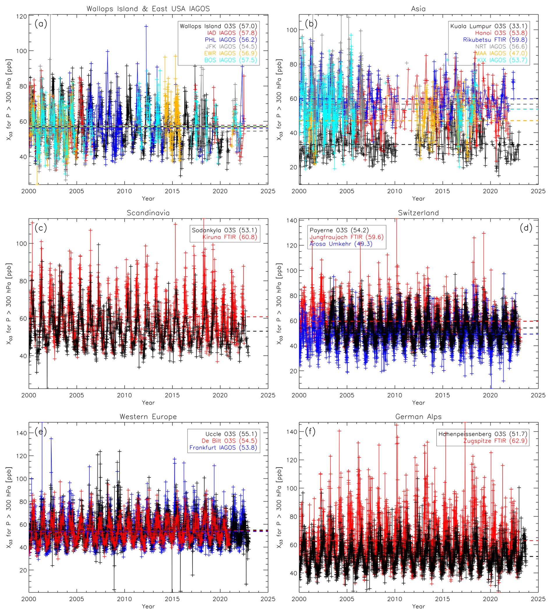
Figure 3Daily mean time series of TrOC extracted and archived in the HEGIFTOM database that are from stations located in a given region. Dashed lines are long-term mean values for each instrument over a 23-year period. Groupings illustrated for (a) the eastern US, (b) Japan and southeast Asia, and (c–f) various parts of Europe. Measurements with time gaps of more than 4 months are not connected with lines.
To investigate these differences between the means in more depth, TrOC intercomparison analyses were made between sites within ±4° in latitude and longitude (identical collocated criterion as in Wang et al., 2024), coincident within 12 h (closest measurements, for L1) or in the same month (L3, monthly mean comparison), and requiring at least 15 coincident measurements. This results in 45 pairwise inter-technique comparisons for all measurements (L1) (see Table S2) and 59 for the monthly means (L3) (see Table S3). Both those analyses confirm the strong positive TrOC bias of FTIR against ozonesondes, IAGOS, and Umkehr (around 5 ppbv on average) at all sites. At all sites except Lauder, Umkehr has a negative bias against all other techniques. The TMF lidar measurements reveal a positive TrOC difference with IAGOS, and the OHP lidar has a positive TrOC difference with Umkehr and ozonesondes (see Table S3). We should, however, note that both those lidars have their lowest data points at around 3 km above the surface, so the best lidar partial ozone column metric for comparison with other techniques is the FTOC between 700 and 300 hPa. With this metric, also positive FTOC differences with IAGOS (TMF) and ozonesondes (OHP) are found.
In our sample sets, there is no consistent bias between IAGOS and ozonesondes (see Tables S2 and S3). This is surprising because a robust positive bias of ozonesonde versus IAGOS ozone measurements has been reported in earlier studies (Zbinden et al., 2013; Staufer et al., 2013, 2014; Tanimoto et al., 2015; Wang et al., 2024; Zang et al., 2024). Note that if DU units are used instead of ppbv for the TrOC comparisons (in Tables S4 and S5), FTIR does not exhibit a consistent bias with the other techniques (as in Garcia et al., 2012), and the lidar mean differences flip to negative at the two sites, but only for the TrOC (not for the FTOC). The negative TrOC bias for Umkehr in DU compared to sondes remains the same. Part of the FTIR and lidar differences may be due to the atmospheric pressure inputs needed to convert between DU and column-averaged mixing ratios. However, the current positive bias of FTIR is well known and explained by the actual bias of 2 %–3 % between the spectroscopic parameters (currently HITRAN 2008) in the infrared range compared to the UV–visible ones. The expected use of HITRAN 2020 in the near future will solve this bias (Gordon et al., 2022; Björklund et al., 2024). In contrast to most of the collocated techniques, lidar ozone measurements are nighttime measurements. Based on the frequent IAGOS FRA profiles, Petetin et al. (2016) found statistically significant diurnal variations in the mean ozone mixing ratios regardless of pressure level, although they quickly decrease with altitude (and hardly discernible above 750 hPa). Therefore, differences in daytime and nighttime mean ozone mixing ratios might partially contribute to the TrOC and FTOC differences between lidar and other collocated techniques. In any case, for trend detection, time-independent biases among techniques are not a major issue, in contrast to drifts. Possible drifts at sites hosting different techniques are discussed later, in Sect. 4.3.1. Finally, in our intercomparison analysis, the best correlations (e.g., linear Pearson correlation coefficients around 0.65 and 0.70 on average for L1 and L3 comparisons, respectively; see Tables S2 to S5) and linear regression slopes closest to 1 are obtained between ozonesondes, IAGOS, and FTIR. A worse agreement between techniques is obtained for the comparisons involving Umkehr, in particular at Lauder.
In Fig. 3a and b, the daily mean time series of sites with large gaps (all IAGOS airports) or relatively short time series (O3S Hanoi, from 2004–2021) are shown. They do not meet the 2000–2022 criteria for trend estimation but remain potential candidates for studying tropospheric ozone variability on a regional scale (Van Malderen et al., 2025).
4.1.2 Geographical distribution for the 2000–2022 period
The overall geographical distribution of mean (column-averaged) tropospheric ozone column, TrOC, over the 2000–2022 period is shown in Fig. 4. For each site, this overall mean value has been calculated from (at least 120) monthly mean values. The lowest mean TrOC values are found in the tropics (< ±15°) and in the Southern Hemisphere (SH), ranging between 25 and 45 ppb. Only at Irene (South Africa) and Ascension Island do the means resemble those of most Northern Hemisphere (NH) sites, i.e., mostly between 50 and 60 ppbv. Cooper et al. (2014) pointed out that satellite TrOC estimates like OMI/MLS TrOC show NH averages exceeding those of the SH average. The higher NH TrOC concentrations are attributed to ozone production from enhanced anthropogenic emissions in the NH and higher rates of stratospheric downwelling (e.g., Griffiths et al., 2021). However, over the tropical Atlantic ozonesondes on multiple oceanographic cruises (Weller et al., 1996; Thompson et al., 2000) it has been shown that year-round tropospheric ozone is greater in the SH than the NH due to fire, lightning, and dynamical influences that bring more FT ozone into the SH (e.g., Moxim and Levy, 2000). Based on an updated OMI/MLS climatology (2004–2019), Elshorbany et al. (2024) found the highest TrOC values over the band of 20–50° N, especially over the eastern coast of the US, southern Europe, and east Asia. Although limited in spatial coverage, sites in those regions are consistent with the highest TrOC values in the HEGIFTOM data (Fig. 4).
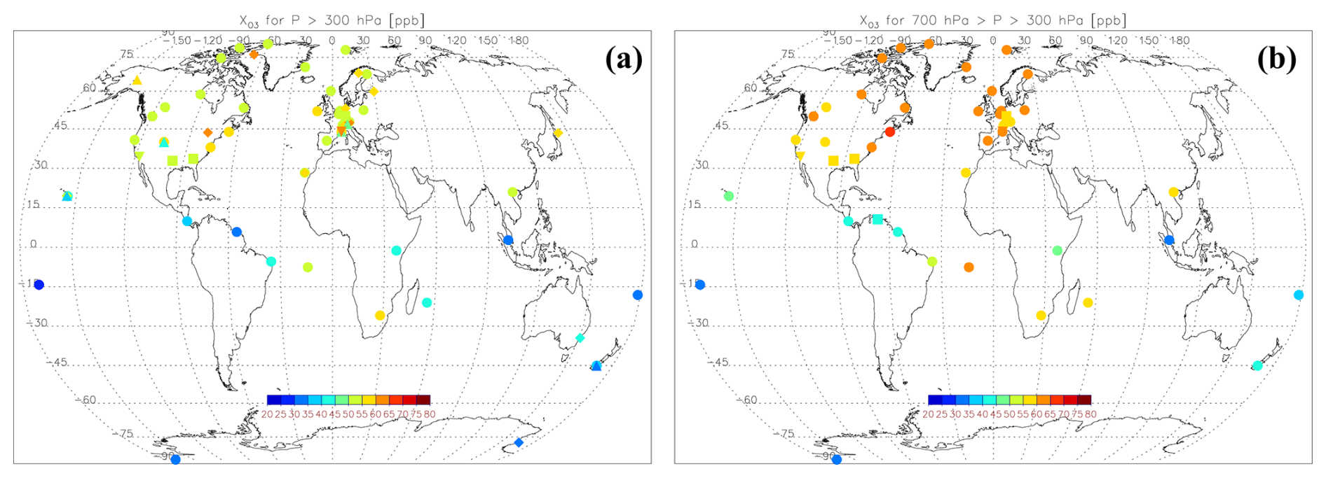
Figure 4Mean (a) TrOC (ppb, surface to 300 hPa) and (b) FTOC (ppb, 700 > p > 300 hPa) at HEGIFTOM sites with at least 120 monthly values in the 2000–2022 period. Circles denote ozonesondes, squares denote IAGOS airports, diamonds denote FTIR, upward triangles denote Umkehr, and downward triangles denote lidar. In the Supplement, a zoom over Europe of this figure is provided (Fig. S2), as well as the mean TrOC and FTOC distributions for DJF and JJA (Fig. S3).
In the Supplement (Fig. S3), we provide mean TrOC mixing ratios for different seasons (DJF and JJA). For the NH sites, TrOC clearly peaks in spring (MAM) and summer (JJA) due to peak stratospheric influence in late winter or spring, peak photochemical production in the summer, and a summertime emission maximum of the important biogenic VOC precursors (Bowman et al., 2022, and references therein). The seasonal variation seen in the SH sites has a well-studied pronounced peak in austral spring (SON), especially across the South Atlantic Ocean and southern Africa. That maximum coincides with the SH peak season for biomass burning and stratosphere-to-troposphere transport (Diab et al., 1996; Thompson et al., 1996; Gaudel et al., 2018, and references therein). These patterns in TrOC variation are observed globally in satellite ozone retrievals (Ziemke et al., 2006) and have been reproduced in chemistry–climate models (e.g., Cooper et al., 2014; Young et al., 2018; Griffiths et al., 2021). Regional dynamics also play a role in ozone over the oceans; e.g., over the tropical western Pacific and east Indian Ocean, minimum TrOC is largely influenced by deep convection (Thompson et al., 2003). Ground-based data also capture anomalous TrOC during extreme events, e.g., an ENSO, that may trigger or suppress fires and modify local convection (Thompson et al., 2001). Note that the reported spatial distribution and seasonal variation of the TrOC amounts are nearly identical when considering the amounts in DU instead of mixing ratios and when the ozone amounts are restricted to the FT only (i.e., column ozone between 700 and 300 hPa).
4.1.3 Climatological ozone changes during (post-)COVID-19
Several studies reported on a decrease in (free-)tropospheric ozone amounts in the years 2020 to 2022 due to the decreased emissions associated with the COVID-19 lockdown restrictions (e.g., Steinbrecht et al., 2021; Chang et al., 2022; Ziemke et al., 2022). Because our trend analyses end in this time frame, a check was made to determine if a tropospheric ozone decline is detectable. In Fig. 5a, we show relative differences between the mean TrOC (surface to 300 hPa) amounts in the years 2020–2022 compared to the years 2000–2019 for all the sites that have enough data in both time periods. For the 2020–2022 period, this means at least 15 monthly mean values and 120 values for the 2000–2019 period (same as for the 2000–2022 period). About 75 % of the sites have lower mean TrOC concentrations during the last 3 years than in the period 2000–2019, accounting for an overall relative decrease of −2.5 %. The decline is very prominent over northern latitudes.
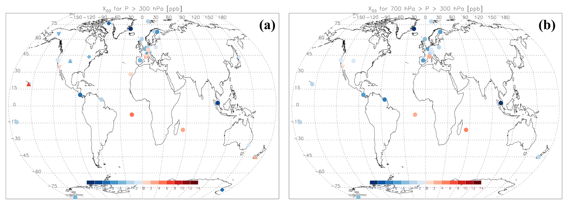
Figure 5Relative change (%) of the mean TrOC (a) and mean FTOC (b) for the time period 2020–2022 versus the period 2000–2019. Only sites which have at least 15, respectively 120, monthly mean values during the 2020–2022, respectively 2000–2019, time periods are retained. Symbols represent the different instruments; same as in Fig. 4.
When split among different seasons, we note that the TrOC decline during the COVID-19 pandemic is strongest during MAM (−5.2 % for 87 % of the sites), followed by JJA (−3.4 % for 70 % of the sites), while there are insignificant TrOC decreases in boreal autumn and winter, with equal amounts of sites experiencing decreases as increases. These numbers are consistent with the observed ozone decreases of approximately 7 % at multiple ozone profile monitoring locations across the northern extratropics, focusing on the 1–8 km column and April–August 2020 (Steinbrecht et al., 2021), and with the observed average decreases in combined satellite TrOC measurements in (boreal) spring–summer 2020 and 2021 in especially the northern midlatitudes (e.g., ∼ −7 %–8 % relative to 2016–2019 average ozone levels in 20–60° N TrOC) in Ziemke et al. (2022). These are attributed largely to decreases in emissions (e.g., NO2 in both years) and reduced photochemical production of ozone in the troposphere, although wildfires may have mitigated the impact after August (in the years 2020 and 2021). When we consider only the FT (700–300 hPa) column amounts (see Fig. 5b), the 2000–2022 reduction from the GB data is even larger (−3.2 % on average, with reduction for 83 % of the sites), with the same dominance in boreal spring (−5.3 %, 92 %) and summer (−4.4 %, 74 %) of the decline. A more systematic examination of the COVID-19 anomaly is presented in trend comparisons in Sect. 4.2.3.
4.1.4 Seasonal cycle changes in tropospheric ozone
Because of the reduction of NH TrOC in boreal spring and summer in recent (post-)COVID years with respect to the other two seasons, the amplitude of the seasonal cycle might be reduced. For example, Ziemke et al. (2022) reported an amplitude reduction in NH satellite tropospheric column ozone by about 15 % in 2020 and 2021 relative to previous years. Clearly, these changes might have an impact on calculations of long-term seasonal trends in tropospheric ozone. Here, we do not limit ourselves to the COVID years, but consider the change in the seasonal cycle between the earliest (2000–2005) and most recent years (2015–2022) in the time series (Fig. 6). Based on model simulations and selected surface and in situ observations, Bowman et al. (2022) found that since the mid-1980s, the amplitude of the seasonal cycle of baseline tropospheric ozone at northern midlatitudes decreased and its maximum shifted to earlier in the year. They attributed those changes to decreasing ozone precursor emissions (VOC and NOx) as a result of air quality control efforts, so that photochemical ozone production in NH summer becomes less dominant in the ozone budget, compared to the period before. In Fig. 6 no obvious consistent change in the phase of the seasonal cycle, represented here as the month of maximum TrOC or FTOC monthly mean, occurs between the 2000–2005 and 2015–2022 time periods. On the other hand, there is a clear overall (i.e., for all but five sites, 90 %) reduction in the amplitude of the seasonal cycle (−12 %) between both time periods. The increase in the minimum annual TrOC values (at 60 % of the sites) and the decrease in the maximum annual TrOC concentrations (at 70 % of the sites) appear to contribute equally to this amplitude reduction. For the FT ozone column (Fig. 6b), we find a (more modest) amplitude reduction in the seasonal cycle (−10 % for 75 % of the sites), which is now predominantly driven by the decrease in the maximum annual FT ozone column amounts. Bowman et al. (2022) attributed the more modest amplitude (and phase) shifts in FT ozone with respect to the surface ozone to the larger influence from the varying anthropogenic emissions in the latter.
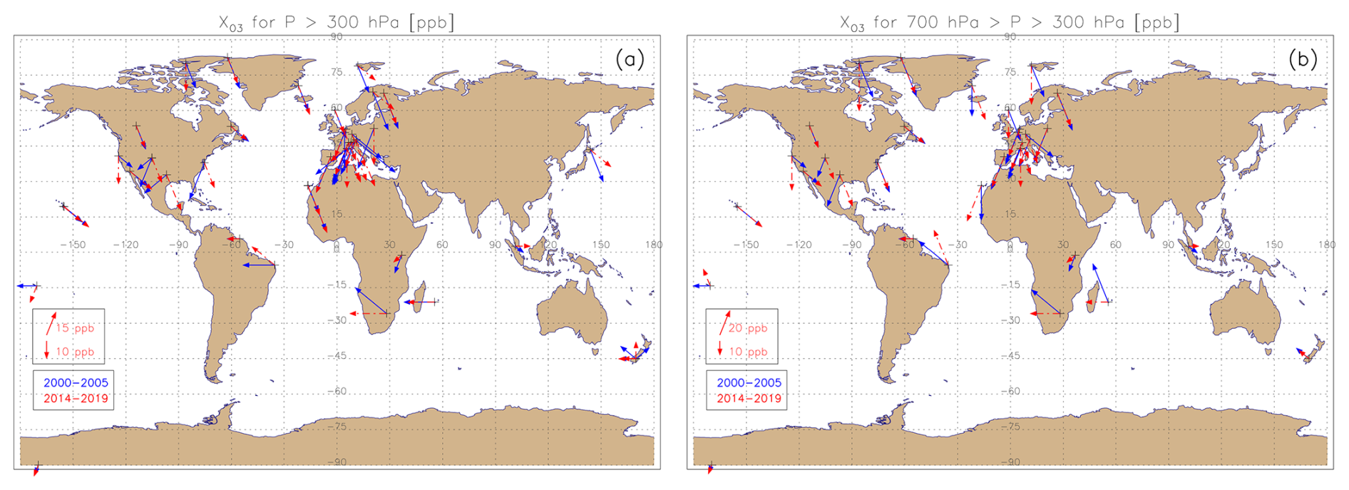
Figure 6Illustration of the mean seasonal cycle for the TrOC (a) and FTOC (b) time series for two different periods: 2000–2005 (blue) and 2015–2022 (red). The amplitude of the seasonal cycle, defined as the difference between the maximum and minimum long-term monthly mean, is represented by the length of the arrow (with units shown in the legend in the lower left of the plots). The phase of the seasonal cycle, defined here as the month with the maximum long-term monthly mean value, is denoted by the direction of the arrow as in a clock: 1 h indicates the phase or maximum long-term monthly mean in January, 2 h indicates February, 3 h indicates March, etc. A zoom over Europe of those figures is provided in Fig. S5.
To be more directly comparable with the Bowman et al. (2022) results, we also calculated the TrOC and FTOC seasonal cycle characteristics of the pre-COVID period 2014–2019 and compared those again with the 2000–2005 seasonal cycle (see Fig. S4). We found that, between those periods, the amplitude reduction is more modest (−6 %) and less general (for 70 % of the sites) than between the 2015–2022 and 2000–2005 periods. The increase in the minimum annual TrOC values (at 65 % of the sites) contributes slightly more than the decrease in the maximum annual TrOC concentrations (at 55 % of the sites). Also for the FTOC, the 2014–2019 amplitude reduction (−3 % for 65 % of the sites) is smaller than for the 2015–2022 period, with equal contributions from increasing minimum and decreasing maximum FT ozone column amounts. From this analysis, we can conclude that the post-COVID-19 period is responsible for about half of the amplitude reduction between 2015–2022 and 2000–2005, without a noticeable seasonal cycle phase shift. This post-COVID-19 seasonal cycle amplitude reduction can be mainly ascribed to a decrease in the maximum annual TrOC/FTOC concentrations (for 79 %/85 % of the sites) during the post-COVID-19 era. This finding is consistent with other observations of tropospheric ozone reductions during the post-COVID-19 period in NH spring and summer time series, mentioned in Sect. 4.1.3 and reported in Ziemke et al. (2022).
The impact of the seasonal cycle amplitude reduction on the trend estimation is rather limited. To this end, we estimated DLM trends for a couple of sites allowing for and without allowing for a changing seasonal cycle. We found insignificant trend differences between both DLM variants.
4.2 Global (partial) tropospheric ozone column trends at ground-based site locations
In this section the results of trends analysis are used to address the following questions.
-
What do TrOC (surface to 300 hPa) trends (2000–2022) look like site to site?
-
How do TrOC trends vary by region? Examine trends longitudinally and with maps.
-
How do TrOC (surface to 300 hPa) trends (2000–2022) compare when computed with QR and MLR?
-
How do FT (free-tropospheric) and TrOC trends compare and why might they differ? Determine FT ozone trends (700–300 hPa column), noting the latter are restricted to the three high-resolution profiling instrument types.
-
How do LTOC trend (surface to 700 hPa) columns (sondes, IAGOS, lidar) compare to TrOC and FTOC trends and why might they differ?
-
What is the impact of the post-COVID19 period (2020–2022) on the calculated trends?
4.2.1 TrOC QR and MLR trends
Figure 7a and b present trends based on QR analyses for the L1 dataset that includes all the data from five instrument types. Displayed are the TrOC changes for the 50th percentile (median, in ppbv O3 per decade, bars for ±2σ) color-coded for the datasets, as a function of latitude (longitude) in Fig. 7a (Fig. 7b). Comparable numbers of sites display positive and negative trends (albeit with sometimes large uncertainties) at all latitudes (Fig. 7a, refer to Table 1 for values) across all longitudes in Fig. 7b; Reunion and the sole Asian station, Kuala Lumpur, bracket a region where trends may be higher. Trends are also strongly positive (and consistently with different techniques) at the high-altitude sites Mauna Loa and Izaña. The principal exception to similarly distributed positive and negative trends is at high latitudes (> 55° N), where negative trends clearly dominate. However, ∼ 42 % of all sites have a TrOC trend non-significantly deviating from zero (p value higher than 0.05). Only the Churchill ozonesonde trend exceeds an absolute value greater than 3 ppbv per decade. These features are apparent in the histogram of median trends in Fig. 7c. Figure 7c indicates distributions among the various instruments. The TrOC trends based on FTIR and ozonesondes tend to be more negative (60 % of their sites) than trends derived from other instruments. The three IAGOS and two lidar sites display only positive trends. There are also positive trends for four of six Umkehr sites, with the sign of the Umkehr trend at some collocated sites differing from the other instrument(s). The FTIR trends are also strong for all but one site, i.e., significantly different from zero. As with Fig. 7c, Fig. 7d conveys a view of global rather than regional TrOC trends (see Fig. 4); however, a similar distribution to Fig. 7c is seen, except that the FTIR larger losses at a few sites are more prominent. It is important to mention here that these trend distributions among the various instruments do not reflect differences due to the different measurement techniques but are driven by the spatial distribution of the different sites for each technique. For instance, the three IAGOS airports are located in urban areas, while the FTIR sample is dominated by remote locations (e.g., polar, high altitude). To screen out the impact of different locations on possible trend differences between techniques, we will have a closer look at the trends of different techniques at collocated or nearby sites in Sect. 4.3.
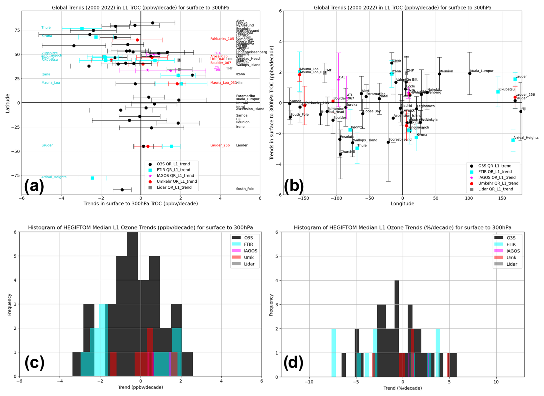
Figure 7(a) Trends for TrOC (in ppbv O3 per decade) over the period 2000–2022 with each station arranged by latitude. Symbols for the five instrument types, color-coded, represent median 50th percentile value. Results shown with +2σ range are based on QR analyses of 55 L1 datasets in the HEGIFTOM archive. (b) Same as panel (a) but arranged by longitude. (c) Histogram of median TrOC trends in ppbv per decade depicted in panels (a) and (b) with color coding for each instrument type. (d) Histogram of same median TrOC trends but in percent per decade based on mean 2000–2022 L1 TrOC values.
Data coverage (columns 7 and 8 in Table 1) is similar among the different techniques, except IAGOS, in terms of percentage of months covered with data. Those means are between 80 % (FTIR) and ∼ 90 % (ozonesondes, Umkehr, lidar), but the average number of daily observations (L2) for each month varies between almost 5 (ozonesondes) and almost 12 (Umkehr), with FTIR and lidar around 9. For IAGOS, where there are only three airports with sufficient coverage to compute trends, the sample numbers (SNs; i.e., number of daily means) are most divergent: ATL and DAL have only ∼ 50 % data coverage, with three to six profiles a month for these months, whereas FRA has around 90 % of months covered, with mean monthly SNs of ∼ 25. This complicates making comparisons among our individual trends. If the strictest SN criteria of Gaudel et al. (2024) or Chang et al. (2024) are applied (> 90 % of months with data, mean monthly SNs > 15), only two HEGIFTOM sites in Fig. 7 or Table 1 would be acceptable for high confidence. These are IAGOS FRA and Umkehr Mauna Loa. In addition, the different techniques have different TrOC uncertainties, with mean values of 2.5 % for lidar, 5.5 % for ozonesonde and IAGOS, 14 % for FTIR, and 15 % for Umkehr (these were estimated by simply averaging the TrOC uncertainties over each site by technique). The statistical methods QR and MLR are compared with the TrOC trends from the monthly mean L3 data in Fig. 8. For none of the sites are the trends significantly different from each other. This is expected because both trend estimates are based on linear regression, use the same proxies for seasonality, and include ENSO. Most sites show not only similar trends, but also similar uncertainties and p values. A comparison of the TrOC trends with L3 data from MLR vs. QR, expressed as ppbv per decade (QR-MLR), shows that the MLR trends are slightly larger, with ∼ 56 % of the differences lying within ± 0.3 ppbv per decade of one another (Fig. 8c). The trend estimation methods also show similar TrOC trend distributions among the various instruments, for both the absolute (ppbv per decade, Fig. 9a and b) and relative (percent per decade, Fig. 9c and d) trends. In Fig. 9d the higher MLR trends are apparent relative to QR: a larger number of positive trends in the MLR at 2 % per decade or higher. In summary, the TrOC trend results for the monthly (L3) QR and MLR data, given the relatively large uncertainty in each calculation, are sufficiently close (Figs. 8 and 9) that we can justify using only one data set and method (QR analysis, L1 data) to address questions about geographical variability in trends.
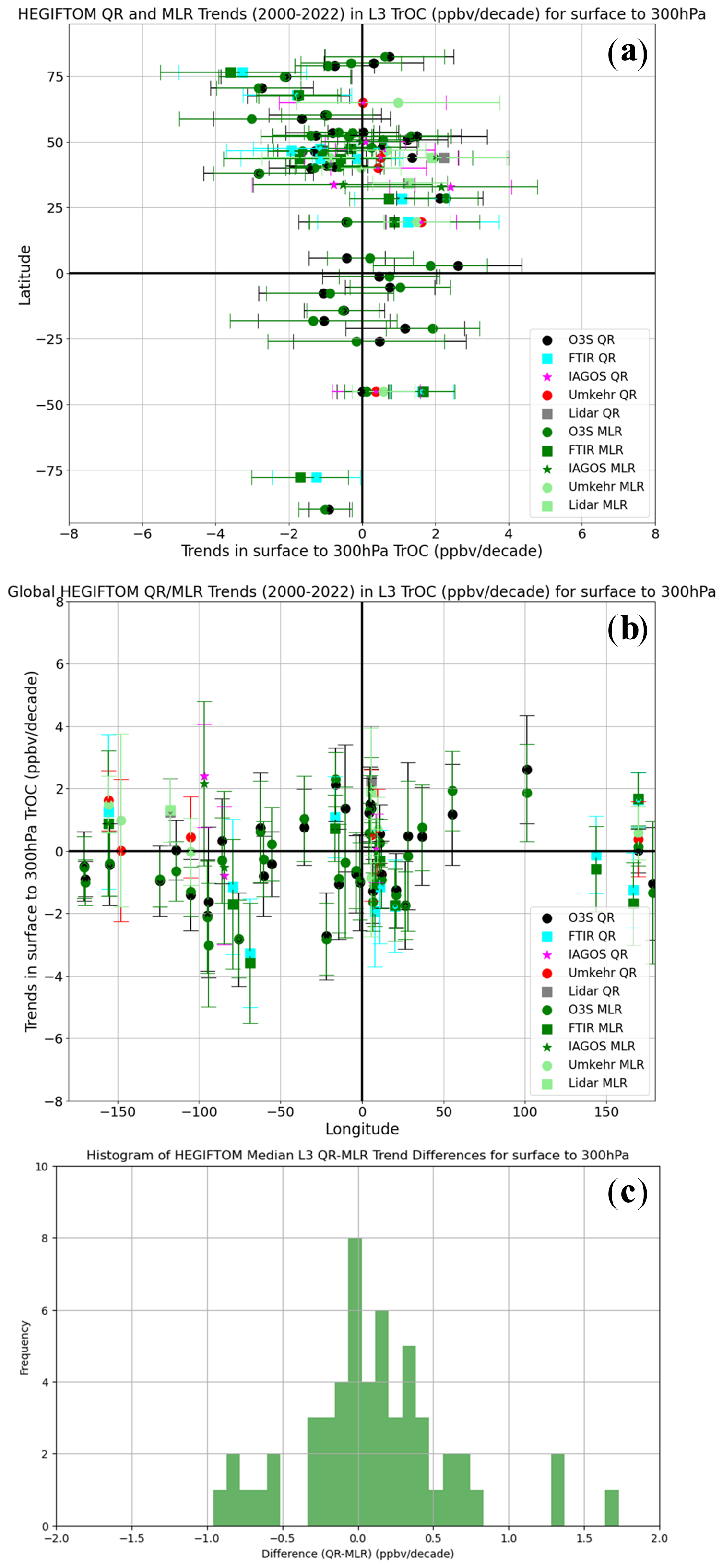
Figure 8(a) Trends for TrOC over the period 2000–2022 with each station arranged by latitude. Results are based on L3 HEGIFTOM data (monthly means) for QR and MLR analyses of 55 datasets. As in Fig. 7, symbols for the five instrument types, color-coded for QR trends, represent median 50th percentile value, shown with +2σ range. For MLR the various instruments have the same symbols as for QR, but colors are in shades of green. (b) Same as panel (a) but arranged by longitude. (c) Histogram of offsets between median trends for all instruments, expressed as QR relative to MLR (QR-MLR), in ppbv O3 per decade.
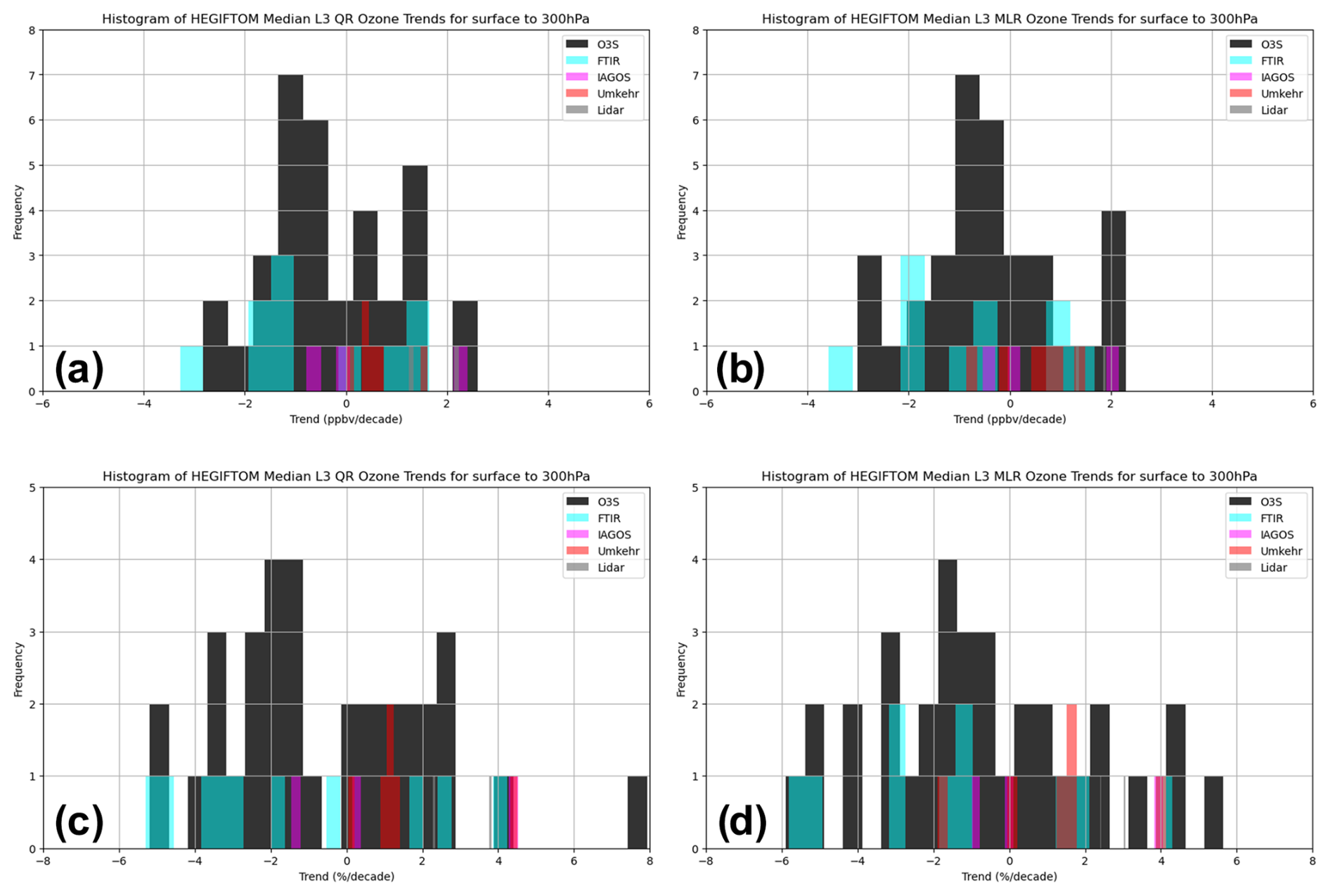
Figure 9Histogram of median TrOC trends for 2000–2022 determined for 55 HEGIFTOM L3 data with color coding for each instrument type. (a) Computed with QR analyses in ppbv per decade and percent per decade in panel (c). (b) Same as panel (a) but for MLR analyses; (d) same as panel (c) but for MLR analyses.
To further study the impact of the monthly SNs on the trend estimations and their uncertainties, we randomly selected for all sites two daily mean (L2) values for each month and calculated the corresponding monthly mean L3 data. Then, we estimated QR and MLR trends for both the original L3 and the subsampled L3 time series. As different combinations of two random samples per month are possible at the bulk of the sites, this trend sensitivity experiment should be executed for a large number of random subsampling strategies. This concept is illustrated in Fig. 6 of Chang et al. (2024), with trends calculated from the Mauna Loa Observatory (free-tropospheric) ozone data set, subsampled randomly and independently over 1000 iterations to a fixed number of samples per month (ranging between 2 and 20). Such an analysis for all our sites clearly falls outside the scope of this paper, and we consider only one subsampled L3 time series. The differences in the trends and their uncertainties with the full L3 time series are presented and shortly described in Table S6 and Fig. S6. In general, the mean absolute trend differences are rather modest (of the order of 0.4–0.5 ppb per decade for both QR and MLR). The most consistent feature of the comparison is the higher trend uncertainties (standard deviations and p values) for the large majority of the sites in the case of the subsampled datasets. We also found that the differences in trend values and trend uncertainties between the two L3 datasets are comparable with those between QR L3 and MLR L3 and between QR L1 and QR L3 for the complete, original time series (see Table 1 and details in Supplement Table S6). We can therefore conclude that the trend uncertainty due to a hypothetical monthly sampling frequency of 2 is comparable to the trend uncertainties associated with the choice of (i) the trend estimation method and (ii) the temporal sampling (all measurements vs. monthly means) for the QR trend estimation.
Figure 10 addresses questions about geographical and instrument variability in TrOC trends by superimposing trends on a global station map. The L1 absolute trends (ppbv per decade) computed with QR (Table 1) for 2000–2022 are illustrated with p values (color-shaded) and arrows for trend magnitudes (median 50th percentile) in Fig. 10a, with details magnified for North America (Fig. S7a–c) and mostly western Europe (Fig. S7b–d). Although TrOC trends in ppbv O3 per decade may seem modest, for regions in which the TrOC is relatively small, e.g., the tropics (Fig. 4), the percent per decade change can be large as in Fig. 10b. When comparing Fig. 10a and b, the largest differences in the trend directions occur in the tropics, e.g., for Kuala Lumpur in East Asia and La Reunion. Figure 10 illustrates variability in trends at individual stations where two or three arrows indicate collocation of multiple instruments (Table 1), typically an ozonesonde launch facility and one or two spectral instruments. A detailed analysis of variable trends at multi-instrument sites or across a region is presented in Sect. 4.3. Figure 10 shows that it is hard to distinguish a consistent geographical trend pattern based on the individual site trends, even for regions where the trends are most significant (p values < 0.05) as in North America and Europe. Except for one Arctic site, all others north of 55° N exhibit negative TrOC trends. Using a model and sonde profiles, Law et al. (2023) noted a “dipole effect” in the vertical tropospheric ozone trends for 1993–2019 of six Arctic stations, i.e., positive trends in winter and summer and negative trends in spring and autumn. This suggests that negative TrOC trends (Fig. 10) reported here may be dominated by negative spring and autumn trends, hypothesized by Law et al. (2023) to originate from decreasing NOx emissions leading to lower FTOC where photochemical production is NOx-limited. In the appendix, Fig. A2, we calculated the monthly TrOC and FTOC 2000–2022 trends for the Arctic sites and found mostly negative trends, except for Alert, with the largest negative trends in springtime. We refer to the appendix for more details.
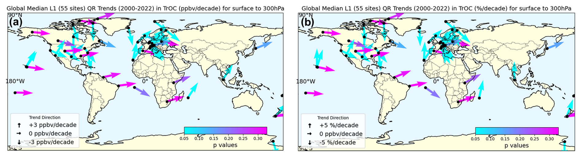
Figure 10Geographical distribution of TrOC trends. (a) Trends for TrOC (in ppbv O3 per decade) over the period 2000–2022 based on QR analyses with HEGIFTOM L1 data. Arrows give the magnitude of the median 50th percentile trend value; note that maximum limits are within ±3 ppbv. Confidence level is indicated with p value denoted by color scale, where p<0.05 is considered high certainty and p>0.3 is considered very low certainty. For multiple arrows at sites with more than one instrument, refer to Table 1 for instrument key. (b) Same as panel (a) except for trends in percent per decade and with the maximum range within ±5 % per decade.
4.2.2 FTOC and LTOC QR trends
Figure 11 is the counterpart to Figs. 7 and 10 except for showing trends in FTOC (column-averaged ozone mixing ratio within 300 < p < 700 hPa) instead of TrOC. The maps (Fig. 11e–f) and longitudinal summary (Fig. 11a–b) based on the QR median (50th percentile) L1 data trends are derived from three instrument types: ozonesondes, IAGOS aircraft profiles, and lidar. The trend estimate values are provided in Table 2. As for TrOC, the range of median trends for FTOC (Fig. 11c) is limited to within ±3 ppbv per decade, except for two sites. To interpret the relationship between FTOC and TrOC trends, fractional trends rather than mixing ratio changes are compared because the column-averaged FTOC mixing ratio is higher than its TrOC counterpart (Fig. 4). These fractional trends are also listed in Table 2.
Table 2Trends for FTOC (ozone mixing ratio within 700 > p>300 hPa) in ppbv per decade and percent (%) per decade based on QR analysis of L1 data for 39 of the 55 datasets in Table 1. Only sites with lidar, ozonesondes, and/or IAGOS ozone profiles collect data in the FT range. Bold trends are those with p<0.05. LTOC trends are also listed for surface to 700 hPa column in ppbv per decade and percent per decade. Only ozonesondes and IAGOS datasets collect data for LTOC.
n/a – not applicable.
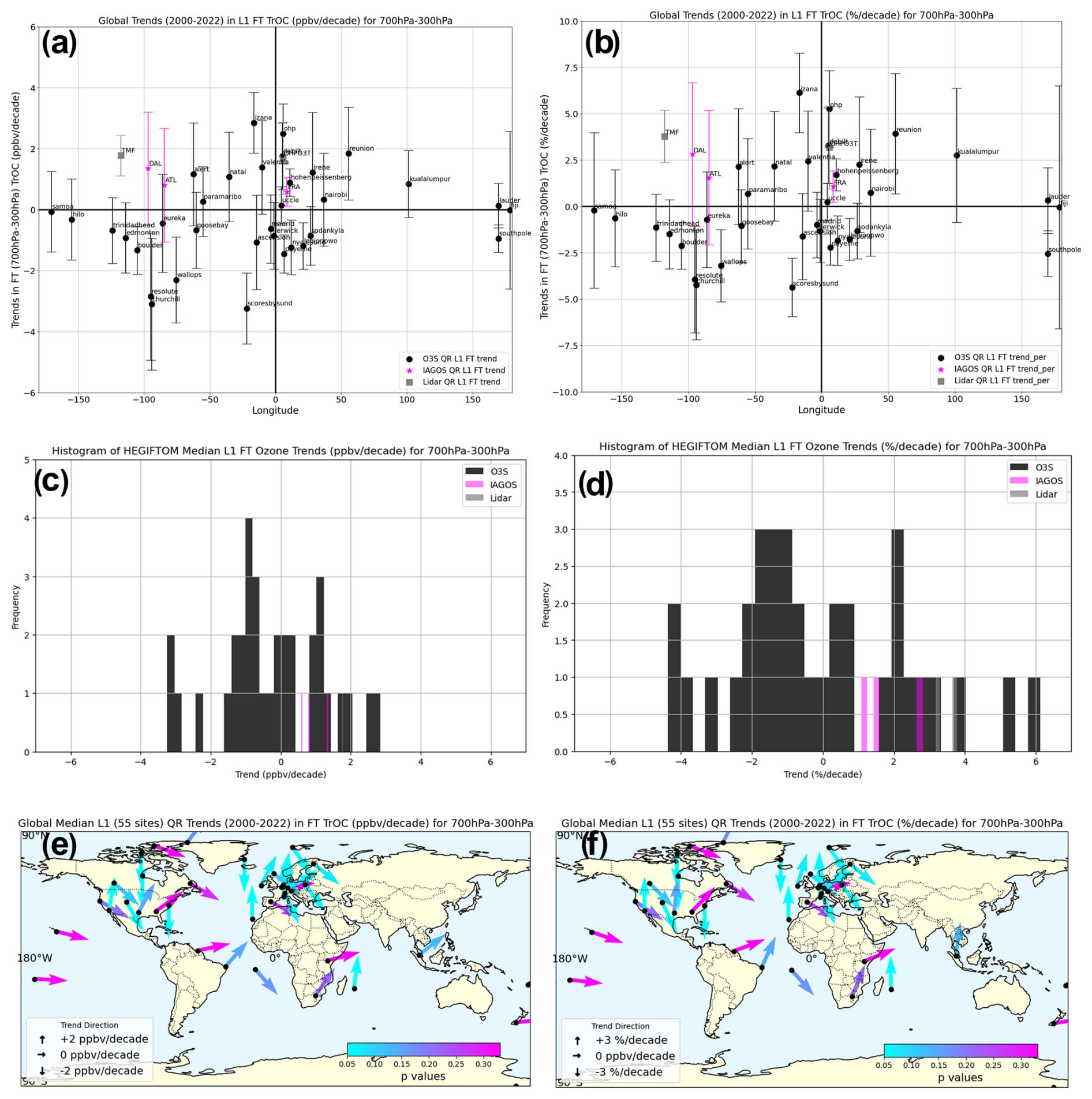
Figure 11(a) Similar to Fig. 7b but for trends for FTOC (change in column ozone, 300 < p < 700 hPa, in ppbv per decade) over the period 2000–2022 based on QR analyses with HEGIFTOM L1 data for three instrument types: ozonesondes, IAGOS profiles, and lidar as a function of longitude. Results for the median 50th percentile and ±2σ are shown. (b) Same as panel (a) but in percent per decade. (c) Histogram showing that most site–instrument datasets are within ±3 ppbv O3 per decade. (d) Same as panel (c) but in percent per decade. (e) Same as Fig. 10a but now for FTOC. (f) Same as panel (e) but in percent per decade.
We first consider the sites with a smaller trend in FTOC relative to TrOC. These include four tropical sites (Reunion Island, Nairobi, Kuala Lumpur, Paramaribo), four urban areas (Frankfurt, Dallas, Uccle, Legionowo), and about half of the Arctic sites (Lerwick, Scoresbysund/Illoqqortoormiut, Resolute, Eureka, Edmonton). For those cases, the relative LTOC trends (surface to 700 hPa, Fig. 12 and Table 2) are higher than the relative TrOC trends, suggesting that local near-surface pollution at the tropical and urban areas contributed to increased TrOC over the 2000–2022 period. Stauffer et al. (2024), writing about tropospheric ozone profile trends derived from Kuala Lumpur and Watukosek for 1998–2022, reported ∼ 6 %–10 % per decade LTOC increases in the February to April period over equatorial southeast Asia during that period. Van Malderen et al. (2021) described higher boundary layer ozone increases than FT ozone trends in Uccle and Frankfurt for the period 1995–2018. For the abovementioned Arctic sites, whose TrOC, LTOC, and FTOC trends are all negative, the larger relative LTOC trends compared to relative TrOC (and hence FTOC) trends (Fig. 12) indicate that the negative free-tropospheric trends, due to mid-tropospheric or low-stratospheric dynamics, are partially offset by the larger LTOC trends for obtaining the TrOC trends.
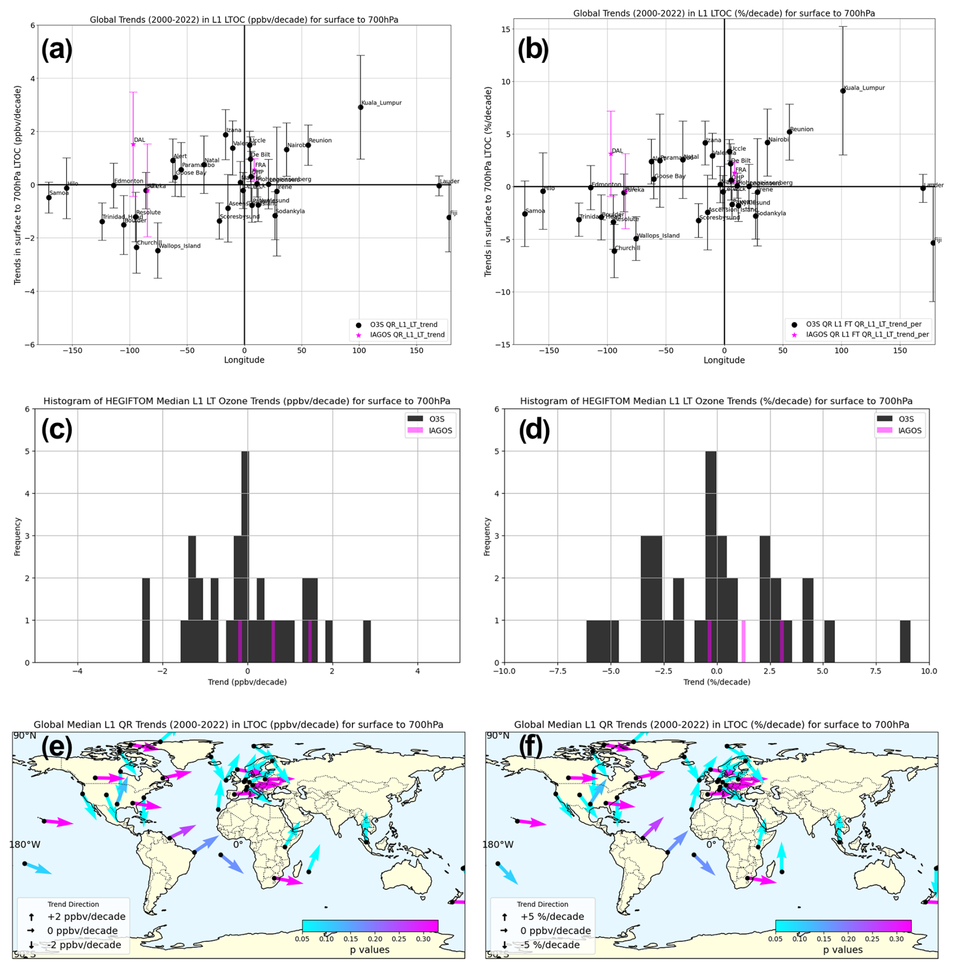
Figure 12Counterpart for Fig. 11 but for trends for LTOC (change in column ozone, 700 < p < surface, in ppbv O3 per decade) over the period 2000–2022 based on QR analyses with HEGIFTOM L1 data plotted versus longitude (a) in ppbv per decade and (b) in percent per decade. For LTOC trends, there are only data from ozonesondes and IAGOS. (c) Histogram showing that most site–instrument datasets are within +2 ppbv O3 per decade. (d) Same as panel (c) but in percent per decade. (e–f) Same as Fig. 11e–f but now for LTOC.
Second, we look at the sites with FTOC increases somewhat greater than TrOC, suggesting imported ozone above the boundary layer. We distinguish two different subsets here: first the one consisting of Irene, Fiji, Samoa, Ascension Island, Hilo, Atlanta, Wallops Island, Trinidad Head, Churchill, Sodankylä, and Ny Ålesund, all sites where LTOC is negative (Fig. 12). Many of these sites are remote locations (all but Atlanta and Irene). Imported pollution in the tropics and subtropics, often downwind of biomass fires, is a reasonable interpretation. This would apply to Ascension and Samoa; for Hilo, seasonal fires and/or industrial pollution from Asia may explain greater FT increases. Another subset is made up of the European ozonesonde sites OHP, Hohenpeissenberg, and De Bilt, which have positive 2000–2022 trends for all partial ozone columns, with the largest relative increase for the FTOC, suggesting that at least some of the column increase is from mid-tropospheric transport.
4.2.3 Post-COVID-19 TrOC trends
As shown in Sect. 4.1.3, the COVID-19 pandemic restrictions led to lower (mean) tropospheric ozone column amounts in the years after 2020, which may be continuing (Blunden and Boyer, 2024). To assess the impact of these tropospheric ozone reductions, we compare the QR L1 2000–2022 trends with the QR L1 trends estimated for the 2000–2019 period. In Fig. 13, the TrOC trends for both time ranges are shown versus latitude and longitude. For the majority of sites (75 %) the 2000–2019 trends are higher than the 2000–2022 trends, by 0.34 ± 0.50 ppbv per decade (or 0.78 ± 1.21 % per decade) on average for the entire sample. There is a trend reduction for all but one Arctic site (Churchill ozonesondes) and for all but one North American site (IAGOS Dallas). In the SH only half of the sites show a trend reduction. In continental Europe, there are a handful of (mainly alpine) sites for which a larger trend is found for 2000–2022 compared to 2000–2019. Overall, there are similar changes in the FTOC: a trend reduction in the 2020–2022 COVID-19 period, indeed for more sites (∼ 80 %), and with similar magnitude (−0.36 ± 0.53 ppb per decade or −0.79 ± 1.43 % per decade) and geographical distribution.
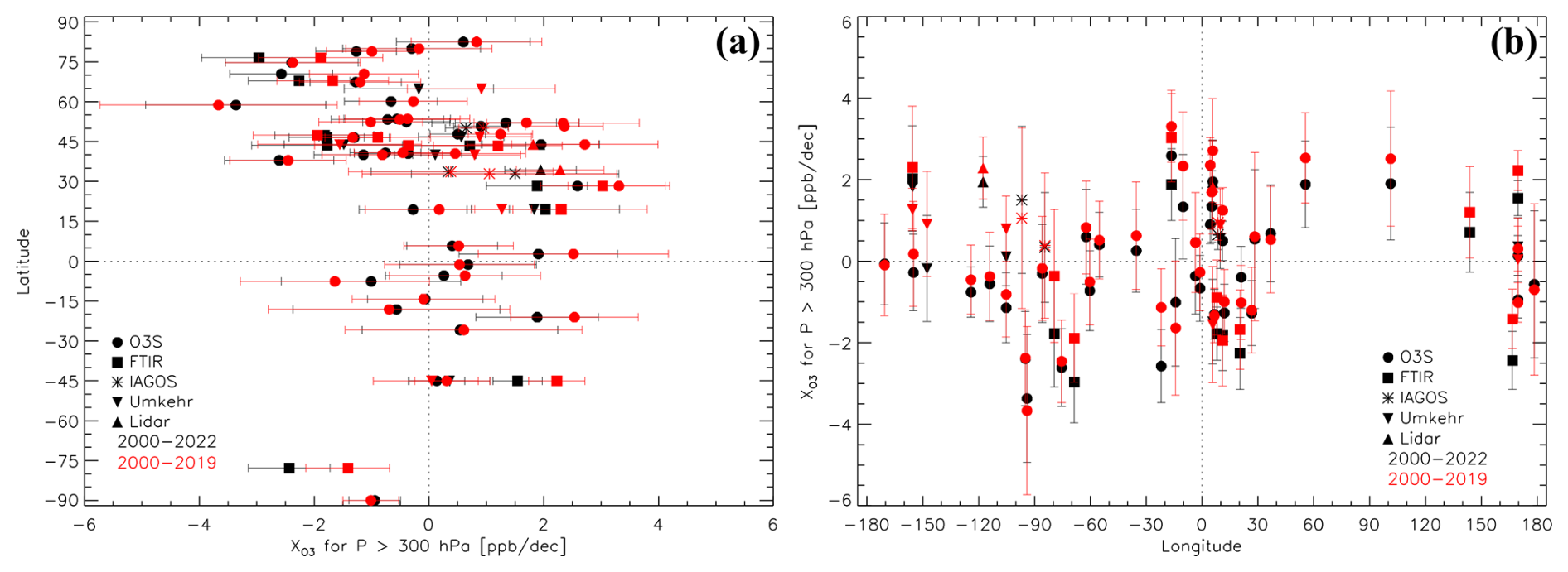
Figure 13TrOC trends (ppb per decade), 2000–2022, computed with L1 data and QR as in Fig. 7 for the five instrument types (black; see legend) as function of latitude (a) and longitude (b). For comparison, trends for the same stations for the pre-COVID-19 period, 2000–2019, are depicted in red.
4.3 Trend comparisons at collocated and nearby sites
Comparisons of QR 2000–2022 trends for TrOC from different techniques at the five collocated sites reveal differences at three of them (Boulder, OHP, and Lauder, Table 1, Fig. 10). For the two other sites, strong positive trends are observed at Izaña from both ozonesondes and FTIR, as well as at Mauna Loa from both Umkehr and FTIR. Similarly, for nearby sites, we observe both agreement and disagreement in trends between techniques. Differences due to instrument technique, e.g., sensitivity of various spectrometers throughout the troposphere, are expected (Petropavlovskikh et al., 2022; Björklund et al., 2024). For some techniques, such factors will vary over the course of a year (e.g., for Umkehr, change in averaging kernels with season and seasonally changing amount of the stray light driven by the amount of total ozone column), and a comparison of monthly averaged trends from the various instruments might be instructive. Differences between the monthly sampling frequency of the techniques can also lead to different trend estimates (e.g., Chang et al., 2024).
In this section, we first try to understand the differences between the median (50th percentile) trends at the collocated and nearby sites by having a closer look at the monthly anomaly time series and the presence of drifts. Then, the DLM technique, which allows for a nonlinear time-varying trend (see Sect. 3.1.3), is used to investigate how the trend changes during 2000–2022 for a subset of those collocated and nearby sites. Finally, monthly averaged trends derived with L3 data and MLR are examined for the collocated sites.
4.3.1 Comparison of trends and monthly anomalies among different techniques at collocated and nearby sites
From Table 1 it is seen that there are five sites with trend estimates for time series from at least two collocated techniques: Boulder (2), Izaña (2), Hawaii (3), OHP (3), and Lauder (3). These sites are used to investigate the consistency of TrOC trends between different techniques, although differences in location (e.g., altitude difference for Izaña and Hawaii), instrumental sensitivity, and temporal sampling (Table S7) might impact the estimated trends. For most of the techniques there is no significant difference among trend estimates at the same site, i.e., they lie within each other's confidence intervals. Notable exceptions are the Umkehr trend at OHP, the ozonesondes at Hawaii (Hilo), and the FTIR at Lauder, which result in significantly different trend values from the other two techniques at those sites (Table 1). It should, however, be noted that the Lauder FTIR trend derived with an improved retrieval strategy is in very close agreement with the trend obtained with the ozonesondes, as shown in detail in Bjorklund et al. (2024). At some sites, trends from collocated techniques even have opposite signs: Hawaii (ozonesondes vs. Umkehr and FTIR), Boulder (ozonesondes vs. Umkehr), and OHP (ozonesondes and lidar vs. Umkehr). As can be seen on the images comparing the monthly anomaly time series of the different techniques at those sites (see Fig. 14), in some of those cases, the overall agreement is rather good (e.g., at Boulder, Lauder, OHP), but outlying periods at the beginning (Umkehr at OHP) or end period (opposite behavior of Umkehr and FTIR at Lauder, drop in Ny Ålesund FTIR) seem to drive the deviating trends. Note that we did not provide trend estimates for the FTIR time series at Boulder and Ny Ålesund; the anomalies are included just for illustration here. From the monthly anomaly time-series differences between two time series, we can determine the drift as the linear regression fit slopes. These might aid in identifying a possible cause for the trend differences, which are summarized in Table S7.
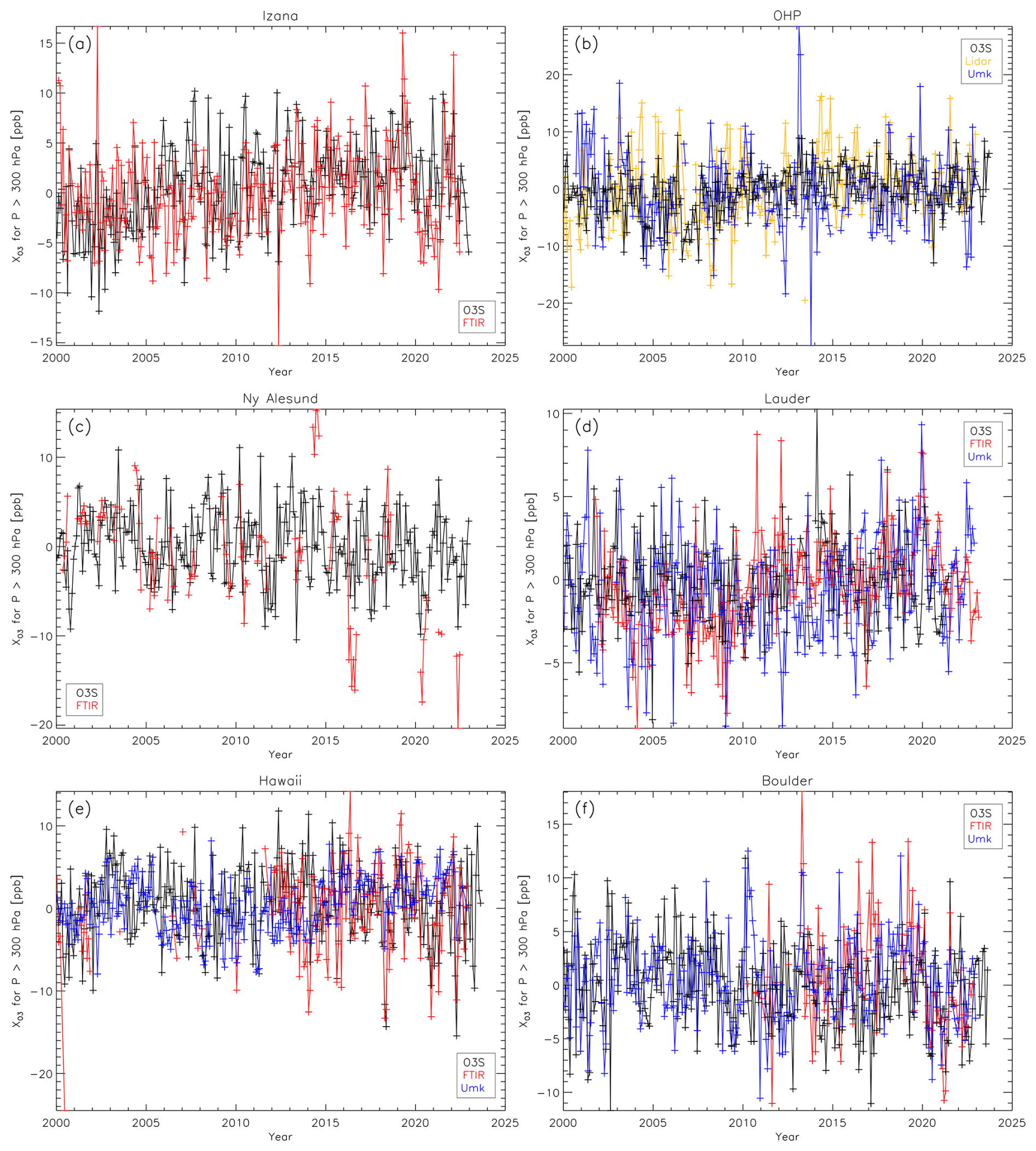
Figure 14Time series for TrOC monthly anomalies, 2000–2022, for six collocated sites, based on the TrOC daily mean time series shown in Fig. 2. The criteria for calculating trends eliminated Boulder FTIR (length of time series) and Ny Ålesund FTIR (sparse sampling). (a) Izaña; (b) OHP; (c) Ny Ålesund; (d) Lauder; (e) Mauna Loa and Hilo, Hawaii; (f) Boulder. Monthly anomalies with time gaps of more than 4 months are not connected with lines.
Figure 15 displays the HEGIFTOM monthly time-series anomalies among neighboring sites, e.g., in the European Arctic (Kiruna and Sodankylä), in the Alps, and in Western Europe (Uccle, De Bilt, Frankfurt). As can be seen, trends at the European Arctic (significantly negative) and Western Europe (significantly positive) sites are fairly consistent with each other (see also Van Malderen et al., 2021, for the latter), whereas the Alpine sites (Fig. 15e and f) reveal both positive (Arosa and Hohenpeissenberg) and negative (Payerne and the high-altitude sites Jungfraujoch and Zugspitze) trends. As some of these sites are high-altitude mountain peak sites (Table S8), the tropospheric ozone column measurements only represent the FT, which might explain differences with lower-altitude sites. Table S8 attempts to explain the trend differences among the various techniques at those sites.
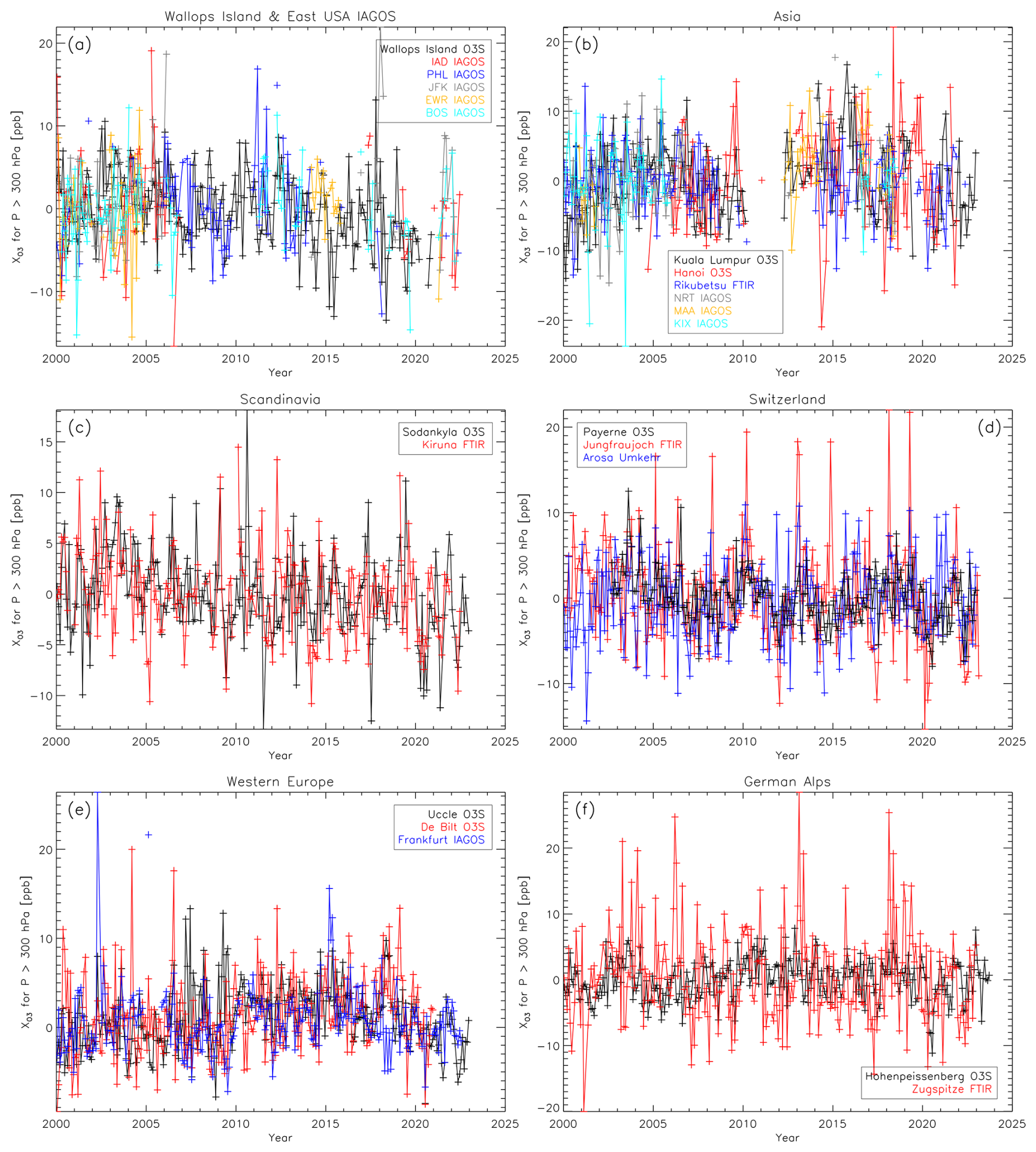
Figure 15Time series for TrOC monthly anomalies, 2000–2022, for regional and nearby instrument clusters illustrated in Fig. 3. (a) eastern US, (b) Japan and southeast Asian sites and airports, (c) two nearby Scandinavian monitoring stations, (d) three nearby Swiss stations, (e) three nearby western Europe ozonesonde stations and airport, and (f) two nearby alpine German stations. For the eastern US and Asian sites, we do not present trend estimates. Monthly anomalies with time gaps of more than 4 months are not connected with lines.
Tables S7 and S8 also summarize the monthly data sampling (in terms of number of days) of the different techniques. The monthly sampling affects the calculation of the monthly anomalies, e.g., in terms of its variability over the time series. For instance, Fig. 15d shows that the monthly anomaly ozonesonde time series at De Bilt (mean monthly launch frequency around 4.3) displays a much larger variability than those from the ozonesonde time series at Uccle (11.8 launches a month) and the IAGOS Frankfurt dataset (24.6) – a factor that may affect both the trend value and its uncertainty (Chang et al., 2020, 2022, 2024); see also the earlier discussion in Sect. 4.2.1. On the other hand, the ozonesonde monthly anomaly time series at OHP and Lauder (Fig. 14b and d, both with launch frequency ∼ 4 times a month) show no more variability than those of the collocated techniques (FTIR, Umkehr, lidar) that have a sampling frequency of at least a factor of 2 higher. Whether or not this is due to undersampling or due to the higher TrOC retrieval uncertainties of some techniques (Umkehr and FTIR, ∼ 15 %) compared to the other techniques (2 % to 6 %) is unclear.
At OHP, the lidar nighttime TrOC trend estimate is very close to the ozonesonde daytime TrOC trend, but those positive trends differ largely from the negative Umkehr daytime trend value. Therefore, at first sight, the impact of sampling during day or night on the trend estimations seems rather limited. However, if we estimate the daytime (76 % of the observations) and nighttime partial ozone column trend estimates from the IAGOS FRA time series, the close-to-zero daytime trends are substantially different from the large positive nighttime trends (between 1.61 and 2.04 ppb per decade, with the largest values for the lower-tropospheric ozone column trends). This finding requires further investigation, e.g., to check the extent of a possible sampling bias (temporal or spatial) between both subsets on the trend estimations. To summarize, apart from clear biases in column-averaged tropospheric ozone column amounts between different techniques (FTIR and Umkehr vs. ozonesondes and IAGOS, Sect. 4.1.1), trend estimates also differ among techniques at some collocated/nearby sites. Besides the impact of the sampling frequency (relatively high for FTIR and Umkehr) and the measurement uncertainty (also higher for FTIR and Umkehr), this might also point to, e.g., Umkehr being sensitive to different parts of the atmospheric column, with contributions from stratospheric ozone.
4.3.2 Comparisons of DLM trends (L3 data) at collocated and nearby sites
To investigate in greater detail the cause for trend differences at collocated and nearby sites, we consider how those trends changed over time in the 2000–2022 period. The DLM technique, described in Sect. 3.1.3, provides this information. As the DLM decadal trends, calculated from the yearly trend values, are not significantly different from the QR and MLR decadal trend estimates used up to now (see Fig. S8), the trend estimates are robust across statistical methods, and the DLM results complement the previously reported results.
Figure 16a–c show the TrOC DLM trend estimates as a function of year for the different measurement techniques at the collocated sites Boulder, Hawaii, and Lauder, respectively. For Boulder (Fig. 16a), the trend estimates are constant with time within ±0.2 ppbv yr−1, with non-significant differences between the always negative (ozonesondes) and close-to-zero (Umkehr) trends. In Hawaii (Fig. 16b), the FTIR trend estimates are constant with time at +0.2 ppbv yr−1, matching the overall QR trend of +2 ppbv per decade (Table S7). After 2014, significant discrepancies are found with significantly positive Umkehr trend estimates and negative ozonesonde trend estimates. The latter may be related to a small total column ozone drop-off in the Hilo ozonesonde dataset (Stauffer et al., 2020, 2022) that is negligible for the other tropical HEGIFTOM data. Hilo is the only station in the analysis where some of the negative trend could also derive from an artifact tropospheric ozone loss caused by SO2 interferences from greater Hawaiian volcanic activity in recent years. At Lauder (Fig. 16c), the positive FTIR DLM trend estimates are significantly different from the negative Umkehr trend estimates around 2009. After 2010, when the Umkehr trend estimates turned positive, they are not significantly different from the O3S and FTIR trend estimates, even after 2020, due to the consideration of the higher uncertainties of the year 2022 for the Umkehr data in the trend estimation.
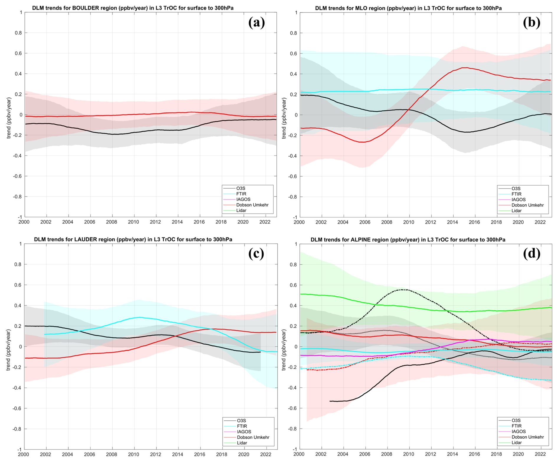
Figure 16DLM trend estimates in ppbv per year for the TrOC for the different measurement techniques at (a) Boulder, (b) Hawaii, (c) Lauder, and (d) OHP and nearby sites Payerne, Hohenpeissenberg, Arosa/Davos, Jungfraujoch, and Zugspitze. IAGOS Frankfurt is also included. For ozonesondes, the dash-dotted line represents OHP, the dotted Hohenpeissenberg, and full line Payerne; for Umkehr the dash-dotted represents OHP and the full line Arosa; for FTIR the dash-dotted represents Jungfraujoch and the full line Zugspitze. Shaded areas represent the ±2σ uncertainties.
In Fig. 16d, we focus on the TrOC DLM trend estimates at OHP and nearby alpine sites (Payerne, Hohenpeissenberg, Zugspitze, Jungfraujoch, Arosa/Davos). Trend estimates derived from Dobson Umkehr (red) and FTIR datasets (cyan) are rather constant with time within ±0.3 ppbv yr−1, although the FTIR Jungfraujoch time series has had increasingly negative trends since 2012. The OHP lidar trend (green) is significantly positive for the entire period. The OHP ozonesonde trend (black, dash-dotted) estimates show, however, an increasing value before 2010 followed by a decreasing trend and are significantly different from all other techniques between 2008–2012. Note that all trend estimate differences are not statistically significant except this one. In 2004–2008 the ozonesonde homogenization applied in Ancellet et al. (2022) is currently under investigation to identify a remaining ozone concentration underestimation when compared with both the stratospheric and the tropospheric OHP ozone lidar. The Payerne ozonesonde trend (full black) is negative for the entire 2002–2022 period but significantly different from zero only until 2009. The differences between the Payerne and Hohenpeissenberg ozonesonde trend estimates are most likely related to the application of the Dobson total ozone normalization factor to the Brewer–Mast ozonesonde at Hohenpeissenberg station (Steinbrecht et al., 2025).
4.3.3 Comparison of monthly MLR trends at collocated sites
Figure 17 displays the monthly trends with 95 % confidence intervals (error bars) over the period 2000–2022 for TrOC at the collocated sites for ozonesondes (O3S in the legend) and the same trend derived from collocated FTIR, lidar, and Umkehr (where available). Because much of the TrOC is located in the FT and large altitude differences exist between techniques at some of those sites (Table S7), the FT trends (4–8 km here) are also graphed. At all stations, the monthly to seasonal trend cycles for TrOC and FTOC from the ozonesondes track one another fairly closely, but there are periods during the year when the other instruments diverge greatly from the sonde trends. For example, the Umkehr monthly trend cycle differs from the ozonesondes at OHP (Fig. 17b), Lauder (Fig. 17c), and Hilo/Mauna Loa (MLO; Fig. 17d). This results in diverging annual MLR TrOC trends at OHP (O3S: 1.96 ± 1.05 ppbv per decade; Umkehr: −0.86 ± 1.88 ppbv per decade) and Hilo/MLO (O3S: −0.41 ± 1.03 ppbv per decade; Umkehr: 1.49 ± 0.91 ppbv per decade). At Lauder, monthly ozonesonde and Umkehr MLR trends that are strongly out of phase coincidentally result in similar annual MLR TrOC trends (O3S: 0.13 ± 0.61 ppbv per decade; Umkehr: 0.58 ± 0.86 ppbv per decade). Monthly MLR analyses show close examination of sub-seasonal differences in trends can reveal important information that is concealed when computing annual average trends. In Appendix A, monthly MLR trends are calculated for some selected nearby stations and airports within the most densely sampled regions represented in the HEGIFTOM database: Europe and North America.
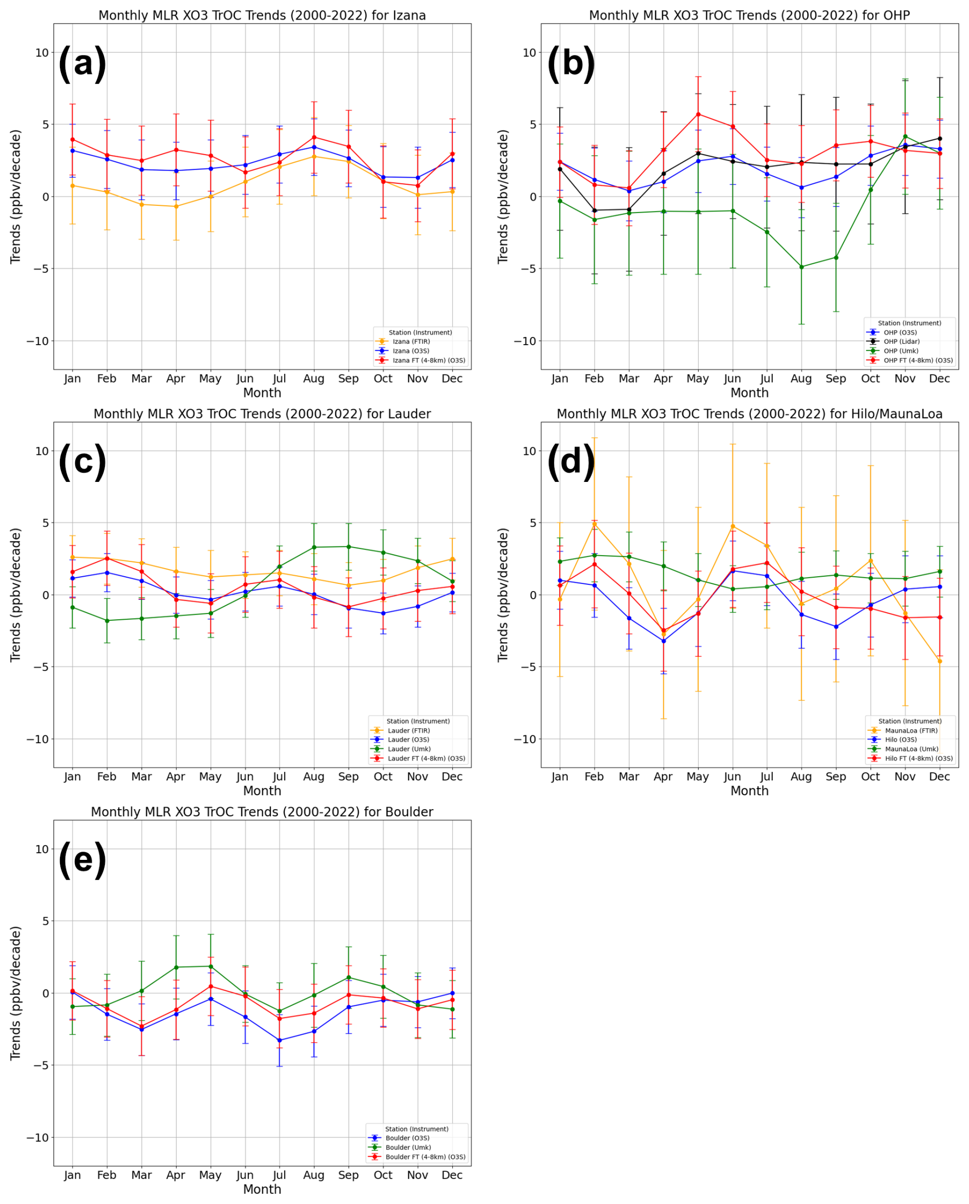
Figure 17Comparison at collocated sites based on TrOC monthly mean trends, 2000–2022. (a) Izaña; (b) OHP; (c) Lauder; (d) Hilo and MLO (Hawaii); (e) Boulder. FTOC (defined between 4 and 8 km here) trends are included for the ozonesonde data (in red).
The TOAR-II HEGIFTOM project to harmonize and evaluate tropospheric ozone measurements from five ground-based instrument types (IAGOS aircraft profiles, ozonesondes, lidar, FTIR, and Umkehr) has been described. The HEGIFTOM data and associated uncertainties, covering more than 350 individual datasets, are available via https://hegiftom.meteo.be/datasets (last access: 8 April 2025). Here, we focused on column ozone in three segments of the troposphere for the period 2000–2022: TrOC (surface to 300 hPa), FT (700 to 300 hPa), and lower troposphere (surface to 700 hPa). A climatology of TrOC is presented along with evidence for an overall (90 % of the sites) reduction in the amplitude of the seasonal cycle (−12 %) during this period, but without an obvious consistent change in the phase of the seasonal cycle.
Analysis of HEGIFTOM data when suitable sample number and time-series endpoint criteria are applied provides comprehensive trends in median TrOC for 55 stations from 2000–2022. The trends were determined using L1 (all data) data from station records with quantile regression (QR). Due to the various sampling protocols for different instruments, some datasets include multiple observations each day (e.g., FTIR, Umkehr, selected airports). Ozone profiles from ozonesondes are often 5 per month or less, while the monthly sampling is around 8 to 12 for lidar, Umkehr, and FTIR. At many airports, gaps are multi-year. Thus, trends with monthly averaged (L3) data were also analyzed using both QR and MLR methods. The main findings are listed below.
-
The three sets of calculations find that TrOC and FTOC median trends nearly all lie within −3 to +3 ppbv per decade. Given the variability of mean TrOC values, these changes range from −4 % per decade predominantly over North America and western Europe to +5 % per decade over much of the tropics and our single SE Asian site. FTOC percentage trends are similar to TrOC, but FTOC increases are greater than those for TrOC when imported FT ozone overlies declining boundary layer ozone in remote locations. In tropical and urban areas, high LTOC trends usually dominate the TrOC increase.
-
Median TrOC trends at all latitudes and across all longitudes include comparable numbers of positive and negative trends (p<0.05), but presented with conventional 2σ error bars about 40 % of the datasets have trend values not different from 0.
-
No geographically consistent patterns emerge from the distribution of TrOC individual site trends, except that 10 out of 11 Arctic sites (> 55° N) display negative TrOC trends.
-
We found evidence for a post-COVID-19 (i.e., the period 2020–2022) impact on the mean TrOC value (−2.5 % on average with respect to 2000–2019), most prominent over NH mid-latitudes and in MAM and JJA. Therefore, for the bulk of the sites (75 %) the 2000–2019 trends are higher than the 2000–2022 trends by 0.34 ± 0.50 ppb per decade on average for the entire sample, for both TrOC and FTOC. These findings are consistent with earlier studies (Steinbrecht et al., 2021; Chang et al., 2022; Ziemke et al., 2022).
-
The advantages of QR for trend detection have received considerable attention in the past decade because of its robustness when extreme values or outliers and gaps are present. However, we found similar trend estimates for QR applied on all observations (L1) and when using QR and MLR on monthly mean values (L3) only. DLM trend estimates for a subset of our sample lie in the same range, and DLM in addition allows us to highlight intermittent periods over which the trend is significant, where trends estimated with the traditional QR and MLR methods do not show any significance.
-
Furthermore, HEGIFTOM analyses demonstrated an essential complementarity of the MLR, QR, and DLM techniques for comprehensive tropospheric ozone trend assessment, between different techniques, at collocated and nearby sites. In addition, monthly trends may pinpoint times of the year when differences among collocated instruments may indicate seasonal impacts on sensing methods.
What is the value of the HEGIFTOM data and our trend results for TOAR II?
-
The individual site time series and trends are a reference for chemistry–climate models being used in TOAR II evaluations of ozone over the period 2000–2022. The trends likewise provide clear constraints for models. Some HEGIFTOM datasets have already been used in previous studies (Christiansen et al., 2022; Wang et al.; 2022; Fiore et al., 2022) to evaluate the tropospheric ozone distribution and trends in atmospheric chemistry models. Although HEGIFTOM data coverage is sparse in some regions, it is important in evaluating model performance to determine whether the observed seasonal and inter-annual variability in TrOC and FTOC in particular is reproduced in each model.
-
The HEGIFTOM data record and trends are also constraints for evaluating evolving satellite products. With a range of new satellite products covering different periods in the 2000–2022 window, the consistency of the HEGIFTOM record is essential for harmonizing and intercalibrating emerging tropospheric ozone satellite products.
-
Our HEGIFTOM trend results are broadly consistent with other TOAR II findings on tropical ozone changes published to date. Stauffer et al. (2024) found a strong seasonal increase over the Kuala Lumpur and Watukosek SHADOZ stations for 1998–2023, which coincides with a decrease in convective activity. Over the Aura satellite era, 2004–2019, roughly half of the SHADOZ period, Gaudel et al. (2024) and Thompson et al. (2025) found a similar FT ozone change of 3 to 5 ppbv per decade over southeast Asia, using a combination of IAGOS aircraft and SHADOZ observations. Our findings also generally agree with the OMI/MLS surface to 300 hPa TrOC trends shown for 2005–2019 in Elshorbany et al. (2024), their Fig. 6, in the sense that North America and Europe are characterized by a mixture of positive and negative trend patterns.
More work needs to be done to update and expand the HEGIFTOM archive and to ensure that the homogenized records are transmitted into long-running archives, e.g., NDACC for the spectral methods and both NDACC and WOUDC for the harmonized ozonesonde profiles. The relative scarcity of publicly available GB data for tropical Asia, Australia, Africa, and South America limits the assessment of tropospheric ozone changes over most of the Southern Hemisphere. Advances in data quality (accuracy and precision) brought about by reprocessing with uniform protocols will continue for instruments within each of the contributing GB networks. This includes updating FTIR records with improved spectroscopic datasets as done in Björklund et al. (2024), the application of new procedures for ozonesonde data processing (Vömel et al., 2020; Smit et al., 2024), and extension of the updated Umkehr tropospheric ozone retrieval (Petropavlovskikh et al., 2022) to other Dobson and Brewer time series, which are expected to enhance overall precision of these records. It was somewhat surprising in this study to find the degree of divergence in trends at multi-instrument sites. The identification of instrumental reasons as well as temporal sampling for the discrepancies has only begun. A follow-up paper (Van Malderen et al., 2025) will use synthesized trends from time series of the different techniques at the collocated sites Lauder and Mauna Loa, hence increasing the monthly sampling frequency at those sites, and will compare those with the trends from the individual time series shown here.
The presence of multi-years gaps and moderate sampling frequency at sites or airports might detract from the current state of assessing tropospheric ozone trends from GB data. Several studies (Chang et al., 2020, 2022, 2024; Gaudel et al., 2024) suggest that 7–15 observations per month, depending on the geographical area, are required to calculate tropospheric ozone trends with high accuracy, where high accuracy is defined as within 5 % of the “true” trend. On the other hand, Christiansen et al. (2022) showed that trends in low-level ozonesondes and TOAR surface sites largely match each other, concluding that ozonesonde sites launching at least three times monthly typically represent trends throughout the vertical column. Likewise, given the desire to reduce trend uncertainty with larger sample sizes and to include more multi-gap datasets, we have investigated approaches for calculating regional tropospheric ozone trends by combining individual site datasets or their trends. This is a challenge because of the extent of nearby site trend differences. Promising results are forthcoming in Van Malderen et al. (2025).
Monthly averaged trends for tropospheric ozone amounts might be suitable for looking at meteorological fields and parameters with pronounced influences on tropospheric ozone seasonal and interannual variability in the FT and lower stratosphere (Randel and Thompson, 2011; Thompson et al., 2011; Thompson et al., 2021; Stauffer et al., 2024). Likewise, divergent trends across stations where ground-based sampling is relatively dense, e.g., sections of Europe and North America, can use monthly patterns to identify which stations are affected by similar or dissimilar meteorological influences on ozone, e.g., as in Stauffer et al. (2024) for equatorial SE Asia. Figure A1 presents trends for TrOC over groups of North American (Fig. A1a) and European (Fig. A1b) stations that have high-confidence (p<0.05) annual MLR trends. The range of QR 50th percentile trends over Europe (Fig. 10) illustrates discrepancies within geographically close stations and airports, including disagreement between trends deduced from two techniques. The monthly MLR TrOC trends for each continent also depict how trends vary across different months of the year. For example, over North America (Fig. A1a), Wallops Island, Boulder, and Churchill ozonesondes show strongly negative trends during Northern Hemisphere summer. However, TMF lidar ozone trends are positive during summer months, likely reflecting differences in summertime pollution trends and long-range transport. Similarly, over Europe (Fig. A1b), OHP and Izaña positive monthly MLR trends from May to August are contrasted by mostly negative trends from all other European sites.
Another example of monthly MLR trends is given in Fig. A2, showing the TrOC (Fig. A2a) and FTOC (A2b) monthly trends for the Arctic sites. All these sites, except Alert, have negative yearly trends, which can be easily deduced from the monthly trend estimates. Using (operational) ozonesonde data from the same sites, Law et al. (2023) noted a dipole effect in the 1993–2019 vertical tropospheric ozone trends, i.e., positive trends in winter and summer and negative trends in spring and autumn. As in Law et al. (2023), the largest negative TrOC and FTOC 2000–2022 trends are evident in springtime (MAM) for most of the sites (with four sites having trends significantly different from zero during one of those months). Also, for most of the sites, the winter (December, January) shows among the largest trends, but positive trend values are hardly reached. In general, the mentioned dipole effect of the tropospheric ozone trends is not clearly present in the TrOC and FTOC 2000–2022 series considered here, and the different Arctic sites display different patterns of seasonal trends. For instance, Resolute has one of the more pronounced seasonalities in the trends, with a peak in negative trends in the spring (April) and a peak in positive trends in the autumn (September and October).
To summarize, the monthly MLR trends essentially serve two purposes: (1) monthly resolved trends allow a closer examination of potential causes for disagreement in annual ozone trends for multi-instrument and closely located stations and (2) monthly trends allow the opportunity to diagnose (although beyond the scope of this paper) the causes of ozone changes that may only be occurring in certain months of the year (e.g., convection as described in Stauffer et al., 2024).
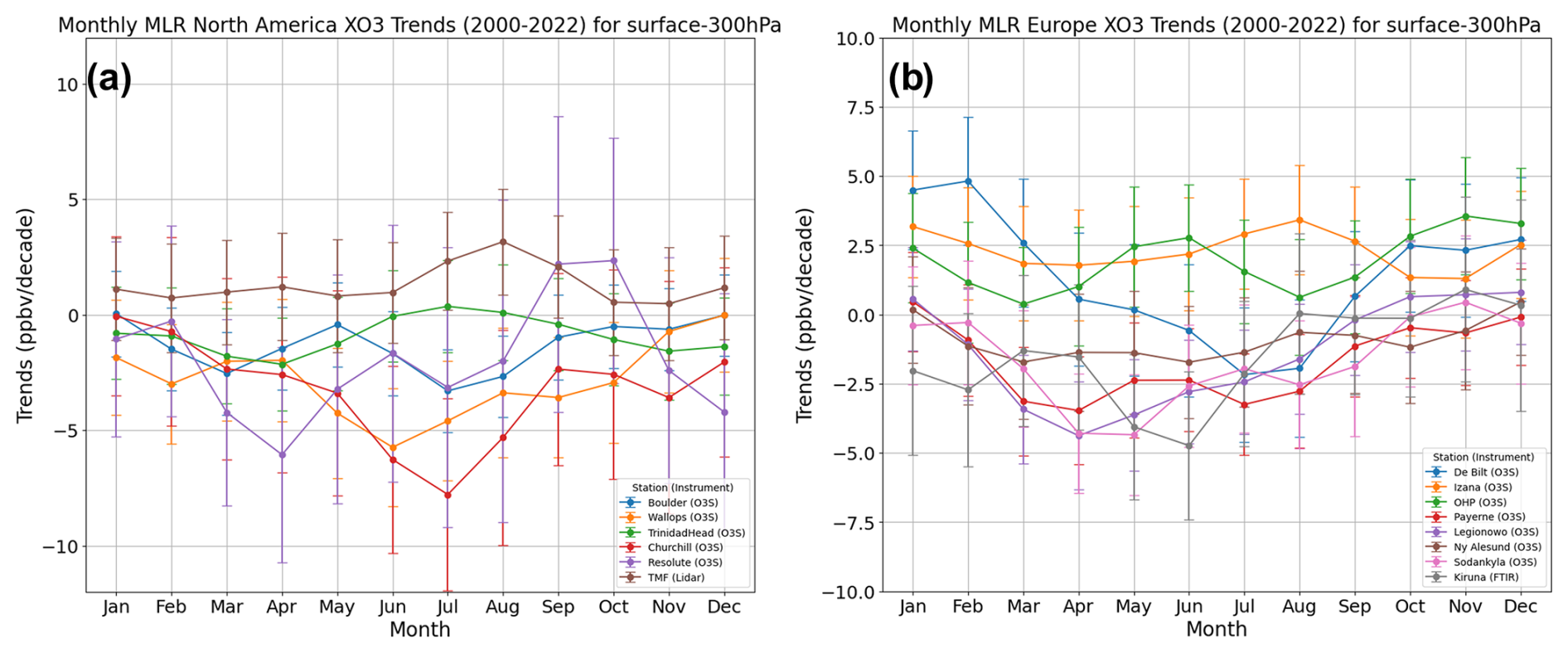
Figure A1Monthly mean TrOC trends computed with MLR for sites with high-confidence (p<0.05) annual MLR trends for (a) North America and (b) Europe.
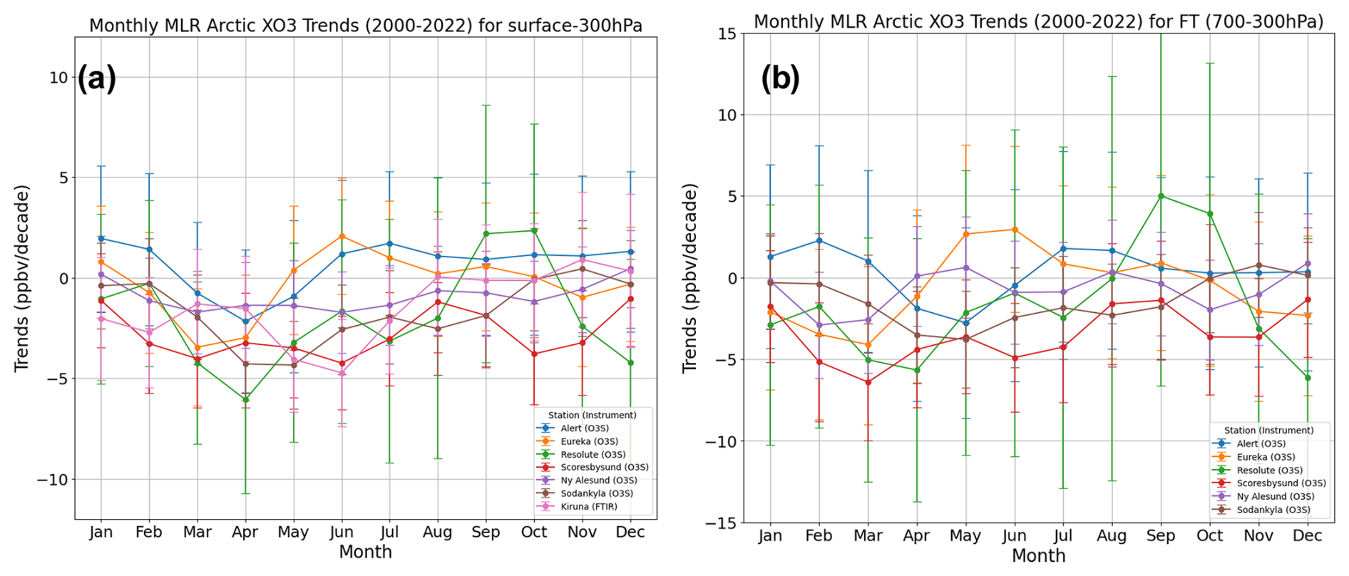
All the (partial) tropospheric ozone column time series used in the paper are available on a public ftp server, with connection details given on the HEGIFTOM website, https://hegiftom.meteo.be/datasets/tropospheric-ozone-columns-trocs (HEGIFTOM TrOC, 2025). The QR trend estimation code can be found at https://github.com/Kai-LanChang/statistical_guidelines and is described in Chang et al. (2023).
The supplement related to this article is available online at https://doi.org/10.5194/acp-25-7187-2025-supplement.
Conceptualization and methodology: RVM, AMT, DEK, RMS, HGJS, EMB, CV, IP, TL, VT, and DWT. Formal analysis and visualization: RVM, AMT, DEK, RMS, and EMB. Data curation: all authors. Writing – original draft preparation: RVM, AMT, RMS, and EMB. Writing – review and editing: all authors.
The contact author has declared that none of the authors has any competing interests.
Publisher’s note: Copernicus Publications remains neutral with regard to jurisdictional claims made in the text, published maps, institutional affiliations, or any other geographical representation in this paper. While Copernicus Publications makes every effort to include appropriate place names, the final responsibility lies with the authors.
This article is part of the special issue “Tropospheric Ozone Assessment Report Phase II (TOAR-II) Community Special Issue (ACP/AMT/BG/GMD inter-journal SI)”. It is a result of the Tropospheric Ozone Assessment Report, Phase II (TOAR-II, 2020–2024).
The FTIR monitoring program at Jungfraujoch was primarily supported by the FRS–FNRS (Brussels, Belgium) and the GAW-CH program of MeteoSwiss (Zürich, Switzerland). Peter Effertz and Irina Petropavlovskikh's research was supported by an NOAA Cooperative Agreement with CIRES, NA17OAR4320101. The National Center for Atmospheric Research is sponsored by the National Science Foundation. The NCAR FTS observation programs at Thule, GR; Boulder, CO; and Mauna Loa, HI, are supported under contract by the National Aeronautics and Space Administration (NASA). The Thule work is also supported by the NSF Office of Polar Programs (OPP). We wish to thank the Danish Meteorological Institute for support at the Thule site and NOAA for support of the MLO site. We are indebted to all the instrument operators, station (co-)PIs, and funding agencies without which the ozone data records used for this research would not have been available. The data used in this publication were obtained as part of the Network for the Detection of Atmospheric Composition Change (NDACC) and are available through the NDACC website https://www.ndacc.org (last access: 20 March 2024). Original ozonesonde data are also stored at https://www.woudc.org (last access: 24 November 2023) and https://tropo.gsfc.nasa.gov/shadoz/ (last access: 24 November 2023). MOZAIC/CARIBIC/IAGOS data were created with support from the European Commission; national agencies in Germany (BMBF), France (MESR), and the UK (NERC); and the IAGOS member institutions (https://www.iagos.org/organisation/members/, last access: 3 July 2025). The participating airlines (Lufthansa, Air France, Austrian, China Airlines, Hawaiian Airlines, Air Canada, Iberia, Eurowings Discover, Cathay Pacific, Air Namibia, Sabena) have supported IAGOS by carrying the measurement equipment free of charge since 1994. The data are available at http://www.iagos.fr (last access: 27 November 2023) thanks to additional support from AERIS.
We are very grateful to Kai-Lan Chang for guidance on applying his QR code and for discussions on statistical recommendations. We also thank Andrey Gaudel, Daan Hubert, and Owen Cooper for their active participation in HEGIFTOM telecoms; for setting the ground for this analysis; and for serving as liaisons to other TOAR-II Focus working groups. We also thank the two anonymous reviewers, whose to-the-point suggestions really improved the analysis, figures, and paper.
This paper was edited by Tim Butler and reviewed by two anonymous referees.
Alsing, J.: dlmmc: Dynamical linear model regression for atmospheric time-series analysis, J. Open Source Softw., 4, 1157, https://doi.org/10.21105/joss.01157, 2019.
Ancellet, G., Papayannis, A., Pelon, J., and Mégie, G.: DIAL tropospheric ozone measurement using a Nd:YAG laser and the Raman shifting technique, J. Atmos. Ocean. Tech., 6, 832–839, 1989.
Ancellet, G., Godin-Beekmann, S., Smit, H. G. J., Stauffer, R. M., Van Malderen, R., Bodichon, R., and Pazmiño, A.: Homogenization of the Observatoire de Haute Provence electrochemical concentration cell (ECC) ozonesonde data record: comparison with lidar and satellite observations, Atmos. Meas. Tech., 15, 3105–3120, https://doi.org/10.5194/amt-15-3105-2022, 2022.
Arosio, C., Sofieva, V., Orfanoz-Cheuquelaf, A., Rozanov, A., Heue, K.-P., Malina, E., Stauffer, R. M., Tarasick, D., Van Malderen, R., Ziemke, J. R., and Weber, M.: Inter-comparison of tropospheric ozone column datasets from combined nadir and limb satellite observations, EGUsphere [preprint], https://doi.org/10.5194/egusphere-2024-3737, 2024.
Balis, D., Koukouli, M., Fountoukidis, P., Fragkos, K., Miyagawa, K., Petropavlovskikh, I., Garane, K., and Bais, A., Umkehr Ozone Profile Analysis and Satellite Validation, Zenodo [report], https://doi.org/10.5281/zenodo.10550453, 2024.
Ball, W. T., Alsing, J., Mortlock, D. J., Rozanov, E. V., Tummon, F., and Haigh, J. D.: Reconciling differences in stratospheric ozone composites, Atmos. Chem. Phys., 17, 12269–12302, https://doi.org/10.5194/acp-17-12269-2017, 2017.
Bass, A. M. and Paur, R. J.: The ultraviolet cross-sections of ozone: I. The measurements, in: Atmospheric Ozone, Proceedings of the Quadrennial Ozone Symposium, held in Halkidiki, Greece, 3–7 September 1984, edited by: Zerefos, C. S. and Ghazi, A., D. Reidel, Norwell, Mass., USA, 606–610, https://doi.org/10.1007/978-94-009-5313-0_120, 1985.
Björklund, R., Vigouroux, C., Effertz, P., García, O. E., Geddes, A., Hannigan, J., Miyagawa, K., Kotkamp, M., Langerock, B., Nedoluha, G., Ortega, I., Petropavlovskikh, I., Poyraz, D., Querel, R., Robinson, J., Shiona, H., Smale, D., Smale, P., Van Malderen, R., and De Mazière, M.: Intercomparison of long-term ground-based measurements of total, tropospheric, and stratospheric ozone at Lauder, New Zealand, Atmos. Meas. Tech., 17, 6819–6849, https://doi.org/10.5194/amt-17-6819-2024, 2024.
Blot, R., Nedelec, P., Boulanger, D., Wolff, P., Sauvage, B., Cousin, J.-M., Athier, G., Zahn, A., Obersteiner, F., Scharffe, D., Petetin, H., Bennouna, Y., Clark, H., and Thouret, V.: Internal consistency of the IAGOS ozone and carbon monoxide measurements for the last 25 years, Atmos. Meas. Tech., 14, 3935–3951, https://doi.org/10.5194/amt-14-3935-2021, 2021.
Bowman, H., Turnock, S., Bauer, S. E., Tsigaridis, K., Deushi, M., Oshima, N., O'Connor, F. M., Horowitz, L., Wu, T., Zhang, J., Kubistin, D., and Parrish, D. D.: Changes in anthropogenic precursor emissions drive shifts in the ozone seasonal cycle throughout the northern midlatitude troposphere, Atmos. Chem. Phys., 22, 3507–3524, https://doi.org/10.5194/acp-22-3507-2022, 2022.
Blunden, J. and Boyer, T. (Eds.): State of the Climate in 2023, Bull. Am. Meteorol. Soc., 105, S1–S484, https://doi.org/10.1175/2024BAMSStateoftheClimate.1, 2024.
Boynard, A., Hurtmans, D., Garane, K., Goutail, F., Hadji-Lazaro, J., Koukouli, M. E., Wespes, C., Vigouroux, C., Keppens, A., Pommereau, J.-P., Pazmino, A., Balis, D., Loyola, D., Valks, P., Sussmann, R., Smale, D., Coheur, P.-F., and Clerbaux, C.: Validation of the IASI FORLI/EUMETSAT ozone products using satellite (GOME-2), ground-based (Brewer–Dobson, SAOZ, FTIR) and ozonesonde measurements, Atmos. Meas. Tech., 11, 5125–5152, https://doi.org/10.5194/amt-11-5125-2018, 2018.
Chang, K.-L., Cooper, O. R., Gaudel, A., Petropavlovskikh, I., and Thouret, V.: Statistical regularization for trend detection: an integrated approach for detecting long-term trends from sparse tropospheric ozone profiles, Atmos. Chem. Phys., 20, 9915–9938, https://doi.org/10.5194/acp-20-9915-2020, 2020.
Chang, K.-L., Schultz, M. G., Lan, X., McClure-Begley, A., Petropavlovskikh, I., Xu, X., and Ziemke, J. R.: Trend detection of atmospheric time series: Incorporating appropriate uncertainty estimates and handling extreme events, Elem. Sci. Anth., 9, 00035, https://doi.org/10.1525/elementa.2021.00035, 2021.
Chang, K.-L., Cooper, O. R., Gaudel, A., Allaart, M., Ancellet, G., Clark, H., Godin-Beekmann, S., Leblanc, T., Van Malderen, R., Nédélec, P., Petropavlovskikh, I., Steinbrecht, W., Stübi, R., Tarasick, D. W., and Torres, C., Impact of the COVID-19 economic downturn on tropospheric ozone trends: An uncertainty weighted data synthesis for quantifying regional anomalies above western North America and Europe, AGU Advances, 3, e2021AV000542, https://doi.org/10.1029/2021AV000542, 2022.
Chang, K. L., Schultz, M. G., Koren, G., and Selke, N.: Guidance note on best statistical practices for TOAR analyses, arXiv [preprint], https://doi.org/10.48550/arXiv.2304.14236, 2023 (code available at: https://github.com/Kai-LanChang/statistical_guidelines, last access: 3 July 2025).
Chang, K.-L., Cooper, O. R., Gaudel, A., Petropavlovskikh, I., Effertz, P., Morris, G., and McDonald, B. C.: Technical note: Challenges in detecting free tropospheric ozone trends in a sparsely sampled environment, Atmos. Chem. Phys., 24, 6197–6218, https://doi.org/10.5194/acp-24-6197-2024, 2024.
Christiansen, B., Jepsen, N., Kivi, R., Hansen, G., Larsen, N., and Korsholm, U. S.: Trends and annual cycles in soundings of Arctic tropospheric ozone, Atmos. Chem. Phys., 17, 9347–9364, https://doi.org/10.5194/acp-17-9347-2017, 2017.
Christiansen, A., Mickley, L. J., Liu, J., Oman, L. D., and Hu, L.: Multidecadal increases in global tropospheric ozone derived from ozonesonde and surface site observations: can models reproduce ozone trends?, Atmos. Chem. Phys., 22, 14751–14782, https://doi.org/10.5194/acp-22-14751-2022, 2022.
Cohen, Y., Petetin, H., Thouret, V., Marécal, V., Josse, B., Clark, H., Sauvage, B., Fontaine, A., Athier, G., Blot, R., Boulanger, D., Cousin, J.-M., and Nédélec, P.: Climatology and long-term evolution of ozone and carbon monoxide in the upper troposphere–lower stratosphere (UTLS) at northern midlatitudes, as seen by IAGOS from 1995 to 2013, Atmos. Chem. Phys., 18, 5415–5453, https://doi.org/10.5194/acp-18-5415-2018, 2018.
Cooper, O. R., Parrish, D. D., Ziemke, J., Balashov, N. V., Cupeiro, M., Galbally, I. E., Gilge, S., Horowitz, L., Jensen, N. R., Lamarque, J.-F., Naik, V., Oltmans, S. J., Schwab, J., Shindell, D. T., Thompson, A. M., Thouret, V., Wang, Y., and Zbinden, R. M.: Global distribution and trends of tropospheric ozone: An observation-based review, Elem. Sci. Anth., 2, 000029, https://doi.org/10.12952/journal.elementa.000029, 2014.
Cooper, O. R., Schultz, M. G., Schröder, S., Chang, K. L., Gaudel, A., Benítez, G. C., Cuevas, E., Fröhlich, M., Galbally, I. E., Molloy, S., and Kubistin, D.: Multi-decadal surface ozone trends at globally distributed remote locations, Elem. Sci. Anth., 8, 23, https://doi.org/10.1525/elementa.420, 2020.
De Mazière, M., Thompson, A. M., Kurylo, M. J., Wild, J. D., Bernhard, G., Blumenstock, T., Braathen, G. O., Hannigan, J. W., Lambert, J.-C., Leblanc, T., McGee, T. J., Nedoluha, G., Petropavlovskikh, I., Seckmeyer, G., Simon, P. C., Steinbrecht, W., and Strahan, S. E.: The Network for the Detection of Atmospheric Composition Change (NDACC): history, status and perspectives, Atmos. Chem. Phys., 18, 4935–4964, https://doi.org/10.5194/acp-18-4935-2018, 2018.
Deshler, T., Mercer, J., Smit, H. G. J., Stübi, R., Levrat, G., Johnson, B. J., Oltmans, S. J., Kivi, R., Davies, J., Thompson, A. M., Witte, J., Schmidlin, F. J., Brothers, G., and Sasaki, T.: Atmospheric comparison of electrochemical cell ozonesondes from different manufacturers, and with different cathode solution strengths: The Balloon Experiment on Standards for Ozonesondes, J. Geophys. Res., 113, D04307, https://doi.org/10.1029/2007JD008975, 2008.
Diab, R. D., Thompson, A. M., Zunckel, M., Coetzee, G. J. R., Combrink, J. B., Bodeker, G. E., Fishman, J., Sokolic, F., McNamara, D. P., Archer, C. B., and Nganga, D.: Vertical ozone distribution over southern Africa and adjacent oceans during SAFARI-92, J. Geophys. Res., 101, 23809–23821, 1996.
Dufour, G., Eremenko, M., Cuesta, J., Ancellet, G., Gill, M., Maillard Barras, E., and Van Malderen, R.: Performance assessment of the IASI-O3 KOPRA product for observing midlatitude tropospheric ozone evolution for 15 years: validation with ozone sondes and consistency of the three IASI instruments, EGUsphere [preprint], https://doi.org/10.5194/egusphere-2024-4096, 2025.
Elshorbany, Y., Ziemke, J. R., Strode, S., Petetin, H., Miyazaki, K., De Smedt, I., Pickering, K., Seguel, R. J., Worden, H., Emmerichs, T., Taraborrelli, D., Cazorla, M., Fadnavis, S., Buchholz, R. R., Gaubert, B., Rojas, N. Y., Nogueira, T., Salameh, T., and Huang, M.: Tropospheric ozone precursors: global and regional distributions, trends, and variability, Atmos. Chem. Phys., 24, 12225–12257, https://doi.org/10.5194/acp-24-12225-2024, 2024.
Eskes, H., Tsikerdekis, A., Ades, M., Alexe, M., Benedictow, A. C., Bennouna, Y., Blake, L., Bouarar, I., Chabrillat, S., Engelen, R., Errera, Q., Flemming, J., Garrigues, S., Griesfeller, J., Huijnen, V., Ilić, L., Inness, A., Kapsomenakis, J., Kipling, Z., Langerock, B., Mortier, A., Parrington, M., Pison, I., Pitkänen, M., Remy, S., Richter, A., Schoenhardt, A., Schulz, M., Thouret, V., Warneke, T., Zerefos, C., and Peuch, V.-H.: Technical note: Evaluation of the Copernicus Atmosphere Monitoring Service Cy48R1 upgrade of June 2023, Atmos. Chem. Phys., 24, 9475–9514, https://doi.org/10.5194/acp-24-9475-2024, 2024.
Fiore, A. M., Hancock, S. E., Lamarque, J.-F., Correa, G. P., Chang, K.-L., Ru, M., Cooper, O. R., Gaudel, A., Polvani, L. M., Sauvage, B., and Ziemke, J. R.: Understanding recent tropospheric ozone trends in the context of large internal variability: A new perspective from chemistry-climate model ensembles, Environ. Res. Clim., 1, 025008, https://doi.org/10.1088/2752-5295/ac9cc2, 2022.
García, O. E., Schneider, M., Redondas, A., González, Y., Hase, F., Blumenstock, T., and Sepúlveda, E.: Investigating the long-term evolution of subtropical ozone profiles applying ground-based FTIR spectrometry, Atmos. Meas. Tech., 5, 2917–2931, https://doi.org/10.5194/amt-5-2917-2012, 2012.
Gaudel, A., Cooper, O. R., Ancellet, G., Barret, B., Boynard, A., Burrows, J. P., Clerbaux, C., Coheur, P.-F., Cuesta, J., Cuevas, E., Doniki, S., Dufour, G., Ebojie, F., Foret, G., Garcia, O., Granados Muños, M. J., Hannigan, J. W., Hase, F., Huang, G., Hassler, B., Hurtmans, D., Jaffe, D., Jones, N., Kalabokas, P., Kerridge, B., Kulawik, S. S., Latter, B., Leblanc, T., Le Flochmoën, E., Lin, W., Liu, J., Liu, X., Mahieu, E., McClure-Begley, A., Neu, J. L., Osman, M., Palm, M., Petetin, H., Petropavlovskikh, I., Querel, R., Rahpoe, N., Rozanov, A., Schultz, M. G., Schwab, J., Siddans, R., Smale, D., Steinbacher, M., Tanimoto, H., Tarasick, D. W., Thouret, V., Thompson, A. M., Trickl, T., Weatherhead, E., Wespes, C., Worden, H. M., Vigouroux, C., Xu, X., Zeng, G., and Ziemke, J.: Tropospheric Ozone Assessment Report: Present-day distribution and trends of tropospheric ozone relevant to climate and global atmospheric chemistry model evaluation, Elem. Sci. Anth., 6, 39, https://doi.org/10.1525/elementa.291, 2018.
Gaudel, A., Cooper, O. R., Chang, K-L., Bourgeois, I., Ziemke, J. R., Strode, S. A. Oman, L. D., Sellitto, P., Nedelec, P., Blot, R., Thouret, V., and Granier, C.: Aircraft observations since the 1990s reveal increases of tropospheric ozone at multiple locations across the Northern Hemisphere, Science Advances, 6, eaba8272, https://doi.org/10.1126/sciadv.aba8272, 2020
Gaudel, A., Bourgeois, I., Li, M., Chang, K.-L., Ziemke, J., Sauvage, B., Stauffer, R. M., Thompson, A. M., Kollonige, D. E., Smith, N., Hubert, D., Keppens, A., Cuesta, J., Heue, K.-P., Veefkind, P., Aikin, K., Peischl, J., Thompson, C. R., Ryerson, T. B., Frost, G. J., McDonald, B. C., and Cooper, O. R.: Tropical tropospheric ozone distribution and trends from in situ and satellite data, Atmos. Chem. Phys., 24, 9975–10000, https://doi.org/10.5194/acp-24-9975-2024, 2024.
Godin-Beekmann, S., Azouz, N., Sofieva, V. F., Hubert, D., Petropavlovskikh, I., Effertz, P., Ancellet, G., Degenstein, D. A., Zawada, D., Froidevaux, L., Frith, S., Wild, J., Davis, S., Steinbrecht, W., Leblanc, T., Querel, R., Tourpali, K., Damadeo, R., Maillard Barras, E., Stübi, R., Vigouroux, C., Arosio, C., Nedoluha, G., Boyd, I., Van Malderen, R., Mahieu, E., Smale, D., and Sussmann, R.: Updated trends of the stratospheric ozone vertical distribution in the 60° S–60° N latitude range based on the LOTUS regression model, Atmos. Chem. Phys., 22, 11657–11673, https://doi.org/10.5194/acp-22-11657-2022, 2022.
Gong, W., Beagley, S. R., Toyota, K., Skov, H., Christensen, J. H., Lupu, A., Pendlebury, D., Zhang, J., Im, U., Kanaya, Y., Saiz-Lopez, A., Sommariva, R., Effertz, P., Halfacre, J. W., Jepsen, N., Kivi, R., Koenig, T. K., Müller, K., Nordstrøm, C., Petropavlovskikh, I., Shepson, P. B., Simpson, W. R., Solberg, S., Staebler, R. M., Tarasick, D. W., Van Malderen, R., and Vestenius, M.: Modelling Arctic Lower Tropospheric Ozone: processes controlling seasonal variations, EGUsphere [preprint], https://doi.org/10.5194/egusphere-2024-3750, 2025.
Gordon, I., Rothman, L., Hargreaves, R., Hashemi, R., Karlovets, E., Skinner, F., Conway, E., Hill, C., Kochanov, R., Tan, Y., Wcisło, P., Finenko, A., Nelson, K., Bernath, P., Birk, M., Boudon, V., Campargue, A., Chance, K., Coustenis, A., Drouin, B., Flaud, J., Gamache, R., Hodges, J., Jacquemart, D., Mlawer, E., Nikitin, A., Perevalov, V., Rotger, M., Tennyson, J., Toon, G., Tran, H., Tyuterev, V., Adkins, E., Baker, A., Barbe, A., Canè, E., Császár, A., Dudaryonok, A., Egorov, O., Fleisher, A., Fleurbaey, H., Foltynowicz, A., Furtenbacher, T., Harrison, J., Hartmann, J., Horneman, V., Huang, X., Karman, T., Karns, J., Kassi, S., Kleiner, I., Kofman, V., Kwabia-Tchana, F., Lavrentieva, N., Lee, T., Long, D., Lukashevskaya, A., Lyulin, O., Makhnev, V., Matt, W., Massie, S., Melosso, M., Mikhailenko, S., Mondelain, D., Müller, H., Naumenko, O., Perrin, A., Polyansky, O., Raddaoui, E., Raston, P., Reed, Z., Rey, M., Richard, C., Tóbiás, R., Sadiek, I., Schwenke, D., Starikova, E., Sung, K., Tamassia, F., Tashkun, S., Vander Auwera, J., Vasilenko, I., Vigasin, A., Villanueva, G., Vispoel, B., Wagner, G., Yachmenev, A., and Yurchenko, S.: The HITRAN2020 molecular spectroscopic database, J. Quant. Spectrosc. Ra., 277, 107949, https://doi.org/10.1016/j.jqsrt.2021.107949, 2022.
Götz, F. W. P., Meetham, A. R., and Dobson, G. M. B.: The vertical distribution of ozone in the atmosphere, Proc. R. Soc. London Ser. A, 145, 416–443, 1934.
Granados-Muñoz, M. J. and Leblanc, T.: Tropospheric ozone seasonal and long-term variability as seen by lidar and surface measurements at the JPL-Table Mountain Facility, California, Atmos. Chem. Phys., 16, 9299–9319, https://doi.org/10.5194/acp-16-9299-2016, 2016.
Griffiths, P. T., Murray, L. T., Zeng, G., Shin, Y. M., Abraham, N. L., Archibald, A. T., Deushi, M., Emmons, L. K., Galbally, I. E., Hassler, B., Horowitz, L. W., Keeble, J., Liu, J., Moeini, O., Naik, V., O'Connor, F. M., Oshima, N., Tarasick, D., Tilmes, S., Turnock, S. T., Wild, O., Young, P. J., and Zanis, P.: Tropospheric ozone in CMIP6 simulations, Atmos. Chem. Phys., 21, 4187–4218, https://doi.org/10.5194/acp-21-4187-2021, 2021.
Harris, N. R. P., Hassler, B., Tummon, F., Bodeker, G. E., Hubert, D., Petropavlovskikh, I., Steinbrecht, W., Anderson, J., Bhartia, P. K., Boone, C. D., Bourassa, A., Davis, S. M., Degenstein, D., Delcloo, A., Frith, S. M., Froidevaux, L., Godin-Beekmann, S., Jones, N., Kurylo, M. J., Kyrölä, E., Laine, M., Leblanc, S. T., Lambert, J.-C., Liley, B., Mahieu, E., Maycock, A., de Mazière, M., Parrish, A., Querel, R., Rosenlof, K. H., Roth, C., Sioris, C., Staehelin, J., Stolarski, R. S., Stübi, R., Tamminen, J., Vigouroux, C., Walker, K. A., Wang, H. J., Wild, J., and Zawodny, J. M.: Past changes in the vertical distribution of ozone – Part 3: Analysis and interpretation of trends, Atmos. Chem. Phys., 15, 9965–9982, https://doi.org/10.5194/acp-15-9965-2015, 2015.
Hase, F., Hannigan, J. W., Coffey, M. T., Goldman, A., Höpfner, M., Jones, N. B., Rinsland, C. P., and Wood, S. W.: Intercomparison of retrieval codes used for the analysis of high-resolution, ground-based FTIR measurements, J. Quant. Spectrosc. Ra., 87, 25–52, 2004.
Hassler, B., Petropavlovskikh, I., Staehelin, J., August, T., Bhartia, P. K., Clerbaux, C., Degenstein, D., Mazière, M. D., Dinelli, B. M., Dudhia, A., Dufour, G., Frith, S. M., Froidevaux, L., Godin-Beekmann, S., Granville, J., Harris, N. R. P., Hoppel, K., Hubert, D., Kasai, Y., Kurylo, M. J., Kyrölä, E., Lambert, J.-C., Levelt, P. F., McElroy, C. T., McPeters, R. D., Munro, R., Nakajima, H., Parrish, A., Raspollini, P., Remsberg, E. E., Rosenlof, K. H., Rozanov, A., Sano, T., Sasano, Y., Shiotani, M., Smit, H. G. J., Stiller, G., Tamminen, J., Tarasick, D. W., Urban, J., van der A, R. J., Veefkind, J. P., Vigouroux, C., von Clarmann, T., von Savigny, C., Walker, K. A., Weber, M., Wild, J., and Zawodny, J. M.: Past changes in the vertical distribution of ozone – Part 1: Measurement techniques, uncertainties and availability, Atmos. Meas. Tech., 7, 1395–1427, https://doi.org/10.5194/amt-7-1395-2014, 2014.
HEGIFTOM TrOC: HEGIFTOM (partial) tropospheric ozone column time series, Van Malderen, R., Vigouroux, C., Petropavlovskikh, I., Leblanc, T., Wolff, P., Thouret, V., HEGIFTOM TrOC [data set], https://hegiftom.meteo.be/datasets/tropospheric-ozone-column-trocs, last access: 8 April 2025.
IPCC: Climate Change 2021: The Physical Science Basis. Contribution of Working Group I to the Sixth Assessment Report of the Intergovernmental Panel on Climate Change, edited by: Masson-Delmotte, V., Zhai, P., Pirani, A., Connors, S. L., Péan, C., Berger, S., Caud, N., Chen, Y., Goldfarb, L., Gomis, M. I., Huang, M., Leitzell, K., Lonnoy, E., Matthews, J. B. R., Maycock, T. K., Waterfield, T., Yelekçi, O., Yu, R., and Zhou, B., Cambridge University Press, Cambridge, United Kingdom and New York, NY, USA, 2023, https://doi.org/10.1017/9781009157896, 2021.
Jones, D., Prates, L., Qu, Z., Cheng, W., Miyazaki, K., Sekiya, T., Inness, A., Kumar, R., Tang, X., Worden, H., Koren, G., and Huijen, V.: Assessment of regional and interannual variations in tropospheric ozone in chemical reanalyses, EGUsphere [preprint], https://doi.org/10.5194/egusphere-2024-3759, 2025.
Keppens, A., Hubert, D., Granville, J., Nath, O., Lambert, J.-C., Wespes, C., Coheur, P.-F., Clerbaux, C., Boynard, A., Siddans, R., Latter, B., Kerridge, B., Di Pede, S., Veefkind, P., Cuesta, J., Dufour, G., Heue, K.-P., Coldewey-Egbers, M., Loyola, D., Orfanoz-Cheuquelaf, A., Maratt Satheesan, S., Eichmann, K.-U., Rozanov, A., Sofieva, V. F., Ziemke, J. R., Inness, A., Van Malderen, R., and Hoffmann, L.: Harmonisation of sixteen tropospheric ozone satellite data records, EGUsphere [preprint], https://doi.org/10.5194/egusphere-2024-3746, 2025.
Koenker, R.: Quantile regression, vol. 38, Cambridge University Press, https://doi.org/10.1017/CBO9780511754098, 2005.
Laine, M., Latva-Pukkila, N., and Kyrölä, E.: Analysing time-varying trends in stratospheric ozone time series using the state space approach, Atmos. Chem. Phys., 14, 9707–9725, https://doi.org/10.5194/acp-14-9707-2014, 2014.
Law, K. S., Hjorth, J. L., Pernov, J. B., Whaley, C. H., Skov, H., Collaud Coen, M., Langner, J., Arnold, S. R, Tarasick, D., Christensen, J., Deushi, M., Effertz, P., Faluvegi, G., Gauss, M., Im, U., Oshima, N., Petropavlovskikh, I., Plummer, D., Tsigaridis, K., Tsyro, S., Solberg, S., and Turnock, S. T.: Arctic tropospheric ozone trends, Geophys. Res. Lett., 50, e2023GL103096, https://doi.org/10.1029/2023GL103096, 2023.
Leblanc, T., Sica, R. J., van Gijsel, J. A. E., Godin-Beekmann, S., Haefele, A., Trickl, T., Payen, G., and Gabarrot, F.: Proposed standardized definitions for vertical resolution and uncertainty in the NDACC lidar ozone and temperature algorithms – Part 1: Vertical resolution, Atmos. Meas. Tech., 9, 4029–4049, https://doi.org/10.5194/amt-9-4029-2016, 2016a.
Leblanc, T., Sica, R. J., van Gijsel, J. A. E., Godin-Beekmann, S., Haefele, A., Trickl, T., Payen, G., and Liberti, G.: Proposed standardized definitions for vertical resolution and uncertainty in the NDACC lidar ozone and temperature algorithms – Part 2: Ozone DIAL uncertainty budget, Atmos. Meas. Tech., 9, 4051–4078, https://doi.org/10.5194/amt-9-4051-2016, 2016b.
Leblanc, T., Brewer, M. A., Wang, P. S., Granados-Muñoz, M. J., Strawbridge, K. B., Travis, M., Firanski, B., Sullivan, J. T., McGee, T. J., Sumnicht, G. K., Twigg, L. W., Berkoff, T. A., Carrion, W., Gronoff, G., Aknan, A., Chen, G., Alvarez, R. J., Langford, A. O., Senff, C. J., Kirgis, G., Johnson, M. S., Kuang, S., and Newchurch, M. J.: Validation of the TOLNet lidars: the Southern California Ozone Observation Project (SCOOP), Atmos. Meas. Tech., 11, 6137–6162, https://doi.org/10.5194/amt-11-6137-2018, 2018.
Lefohn, A. S., Malley, C. S., Smith, L., Wells, B., Hazucha, M., Simon, H., Naik, V., Mills, G., Schultz, M. G., Paoletti, E., and De Marco, A.: Tropospheric ozone assessment report: Global ozone metrics for climate change, human health, and crop/ecosystem research, Elem. Sci. Anth., 6, 28, https://doi.org/10.1525/elementa.279, 2018.
Logan, J. A., Staehelin, J., Megretskaia, I. A., Cammas, J.-P., Thouret, V., Claude, H., De Backer, H., Steinbacher, M., Scheel, H.-E., Stübi, R., Fröhlich, M., and Derwent, R.: Changes in ozone over Europe since 1990: analysis of ozone measurements from sondes, regular aircraft (MOZAIC) and alpine surface sites, J. Geophys. Res., 117, D09301, https://doi.org/10.1029/2011JD016952, 2012.
Maillard Barras, E., Haefele, A., Stübi, R., Jouberton, A., Schill, H., Petropavlovskikh, I., Miyagawa, K., Stanek, M., and Froidevaux, L.: Dynamical linear modeling estimates of long-term ozone trends from homogenized Dobson Umkehr profiles at Arosa/Davos, Switzerland, Atmos. Chem. Phys., 22, 14283–14302, https://doi.org/10.5194/acp-22-14283-2022, 2022.
Maratt Satheesan, S., Eichmann, K.-U., Weber, M., Van Malderen, R., Stauffer, R., and Tarasick, D.: Extension of the S5P-TROPOMI CCD tropospheric ozone retrieval to mid-latitudes, EGUsphere [preprint], https://doi.org/10.5194/egusphere-2025-306, 2025.
Marenco, A., Thouret, V., Nédélec, P., Smit, H., Helten, M., Kley, D., Karsher, F., Simon, P., Law, K., Pyle, J., Poschmann, G., Von Wrede, R., Hume, C., and Cook, T.: Measurement of ozone and water vapour by Airbus in-service aircraft : The MOZAIC airborne programme, an overview, J. Geophys. Res., 103, 25631–25642, 1998.
McDermid, I. S., Beyerle, G., Haner, D. A., and Leblanc, T.: Redesign and improved performance of the tropospheric ozone lidar at the Jet Propulsion Laboratory Table Mountain Facility, Appl. Opt., 41, 7550–7555, 2002.
Mégie, G., Allain, J. Y., Chanin, M. L., and Blamont, J. E.: Vertical Profile of Stratospheric Ozone by Lidar Sounding from Ground, Nature, 270, 329–331, 1977.
Mills, G., Pleijel, H., Malley, C. S., Sinha, B., Cooper, O. R., Schultz, M. G., Neufeld, H. S., Simpson, D., Sharps, K., Feng, Z., and Gerosa, G.: Tropospheric Ozone Assessment Report: Present-day tropospheric ozone distribution and trends relevant to vegetation, Elem. Sci. Anth., 6, 47, https://doi.org/10.1525/elementa.302, 2018.
Monks, P. S., Archibald, A. T., Colette, A., Cooper, O., Coyle, M., Derwent, R., Fowler, D., Granier, C., Law, K. S., Mills, G. E., Stevenson, D. S., Tarasova, O., Thouret, V., von Schneidemesser, E., Sommariva, R., Wild, O., and Williams, M. L.: Tropospheric ozone and its precursors from the urban to the global scale from air quality to short-lived climate forcer, Atmos. Chem. Phys., 15, 8889–8973, https://doi.org/10.5194/acp-15-8889-2015, 2015.
Moxim, W. J. and Levy II, H.: A model analysis of tropical South Atlantic Ocean tropospheric ozone maximum: The interaction of transport and chemistry, J. Geophys. Res., 105, 17393–17415, https://doi.org/10.1029/2000JD900175, 2000.
Nédélec, P., Blot, R., Boulanger, D., Athier, G., Cousin, J.-M., Gautron, B., Petzold, A., Volz-Thomas, A., and Thouret, V.: Instrumentation on commercial aircraft for monitoring the atmospheric composition on a global scale: the IAGOS system, technical overview of ozone and carbon monoxide measurements, Tellus B, 67, 27791, https://doi.org/10.3402/tellusb.v67.27791, 2015.
Nilsen, K., Kivi, R., Laine, M. ,Poyraz, D., Van Malderen, R., von der Gathen, P., Tarasick, D. W., Thölix, L., and Jepsen, N.: Time-varying trends from Arctic ozonesonde time series in the years 1994–2022, Sci. Rep. 14, 27683, https://doi.org/10.1038/s41598-024-75364-7, 2024.
Oltmans, S. J., Lefohn, A. S., Shadwick, D., Harris, J. M., Scheel, H. E., Galbally, I., Tarasick, D. W., Johnson, B. J., Brunke, E.-G., Claude, H., Zeng, G., Nichol, S., Schmidlin, F., Davies, J., Cuevas, E., Redondas, A., Naoe, H., Nakano, T., and Kawasato, T.: Recent tropospheric ozone changes – A pattern dominated by slow or no growth, Atmos. Environ., 67, 331–351, https://doi.org/10.1016/j.atmosenv.2012.10.057, 2013.
Pennington, E. A., Osterman, G. B., Payne, V. H., Miyazaki, K., Bowman, K. W., and Neu, J. L.: Quantifying biases in TROPESS AIRS, CrIS, and joint AIRS+OMI tropospheric ozone products using ozonesondes, EGUsphere [preprint], https://doi.org/10.5194/egusphere-2024-3701, 2024.
Petetin, H., Thouret, V., Athier, G., Blot, R., Boulanger, D., Cousin, J.-M., Gaudel, A., Nédélec, P., and Cooper, O.: Diurnal cycle of ozone throughout the troposphere over Frankfurt as measured by MOZAIC-IAGOS commercial aircraft, Elem. Sci. Anth., 4, 000129, https://doi.org/10.12952/journal.elementa.000129, 2016.
Petropavlovskikh, I., Bhartia, P. K., and DeLuisi, J.: New Umkehr ozone profile retrieval algorithm optimised for climatological studies, Geophys. Res. Lett., 32, L16808, https://doi.org/10.1029/2005GL023323, 2005.
Petropavlovskikh, I., Evans, R., McConville, G., Oltmans, S., Quincy, D., Lantz, K., Disterhoft, P., Stanek, M., and Flynn, L.: Sensitivity of Dobson and Brewer Umkehr ozone profile retrievals to ozone cross-sections and stray light effects, Atmos. Meas. Tech., 4, 1841–1853, https://doi.org/10.5194/amt-4-1841-2011, 2011.
Petropavlovskikh, I., Miyagawa, K., McClure-Beegle, A., Johnson, B., Wild, J., Strahan, S., Wargan, K., Querel, R., Flynn, L., Beach, E., Ancellet, G., and Godin-Beekmann, S.: Optimized Umkehr profile algorithm for ozone trend analyses, Atmos. Meas. Tech., 15, 1849–1870, https://doi.org/10.5194/amt-15-1849-2022, 2022.
Petzold, A., Thouret, V., Gerbig, C., Zahn, A., Brenninkmeijer, C. A. M., Gallagher, M., Hermann, M., Pontaud, M., Ziereis, H., Boulanger, D., Marshall, J., Nédélec, P., Smit, H. G. J., Friess, U., Flaud, J.-M., Wahner, A., Cammas, J.-P., Volz-Thomas, A., and Team, I.: Global-scale atmosphere monitoring by in-service aircraft – current achievements and future prospects of the European Research Infrastructure IAGOS, Tellus B, 67, 28452, https://doi.org/10.3402/tellusb.v67.28452, 2015.
Randel, W. J. and Thompson, A. M.: Interannual variability and trends in tropical ozone derived from SHADOZ ozonesondes and SAGE II satellite data. J. Geophys. Res., 116, D07303, https://doi.org/10.1029/2010JD015195, 2011.
Rodgers, C. D.: Inverse methods for atmospheric sounding: Theory and Practice, Series on Atmospheric, Oceanic and Planetary Physics – Vol. 2, World Scientific Publishing Co., Singapore, https://doi.org/10.1142/3171, 2000.
Smit, H. G. J., Sträter, W., Johnson, B. J., Oltmans, S. J., Davies, J., Tarasick, D. W., Högger, B., Stübi, R., Schmidlin, F. J., Northam, T., Thompson, A. M., Witte, J. C., Boyd, I., and Posny, F.: Assessment of the performance of ECC ozonesondes under quasi-flight conditions in the environmental simulation chamber: Insights from the Jülich Ozone Sonde Intercomparison Experiment (JOSIE), J. Geophys. Res., 112, D19306, https://doi.org/10.1029/2006JD007308, 2007.
Smit, H. G. J. and O3S-DQA Panel: Guidelines for Homogenization of Ozonesonde Data, SI2N/O3S-DQA Activity as part of “Past Changes in the Vertical Distribution of Ozone Assessment”, https://www.wccos-josie.org/en/o3s-dqa/ (last access: 6 November 2024), 2012.
Smit, H. G. J. and the ASOPOS Panel: Quality Assurance and Quality Control for Ozonesonde Measurements in GAW, WMO Global Atmosphere Watch Report Series, No. 201, World Meteorological Organization, Geneva, https://library.wmo.int/idurl/4/55131 (last access: 6 November 2024), 2014.
Smit, H. G. J., Thompson, A. M., and the ASOPOS 2.0 Panel: Ozonesonde Measurement Principles and Best Operational Practices, WMO Global Atmosphere Watch Report Series, No. 268, World Meteorological Organization, Geneva, https://library.wmo.int/idurl/4/57720 (last access: 10 December 2023), 2021.
Smit, H. G. J., Poyraz, D., Van Malderen, R., Thompson, A. M., Tarasick, D. W., Stauffer, R. M., Johnson, B. J., and Kollonige, D. E.: New insights from the Jülich Ozone Sonde Intercomparison Experiment: calibration functions traceable to one ozone reference instrument, Atmos. Meas. Tech., 17, 73–112, https://doi.org/10.5194/amt-17-73-2024, 2024.
Smit, H. G. J., Galle, T., Blot, R., Obersteiner, F., Nédélec, P., Zahn, A., Cousin, J.-M., Bundke, U., Petzold, A., Thouret, V., and Clark, H.: Intercomparison of IAGOS-CORE, IAGOS-CARIBIC and WMO/GAW-WCCOS Ozone Instruments at the Environmental Simulation Facility at Jülich, Germany, EGUsphere [preprint], https://doi.org/10.5194/egusphere-2024-3760, 2025.
SPARC/IO3C/GAW: SPARC/IO3C/GAW report on long-term ozone trends and uncertainties in the stratosphere, in: SPARC report No. 9, GAW report No. 241, edited by: Petropavlovskikh, I., Godin-Beekmann, S., Hubert, D., Damadeo, R., Hassler, B., and Sofieva, V., WCRP-17/2018, https://doi.org/10.17874/f899e57a20b, 2019.
Staufer, J., Staehelin, J., Stübi, R., Peter, T., Tummon, F., and Thouret, V.: Trajectory matching of ozonesondes and MOZAIC measurements in the UTLS – Part 1: Method description and application at Payerne, Switzerland, Atmos. Meas. Tech., 6, 3393–3406, https://doi.org/10.5194/amt-6-3393-2013, 2013.
Staufer, J., Staehelin, J., Stübi, R., Peter, T., Tummon, F., and Thouret, V.: Trajectory matching of ozonesondes and MOZAIC measurements in the UTLS – Part 2: Application to the global ozonesonde network, Atmos. Meas. Tech., 7, 241–266, https://doi.org/10.5194/amt-7-241-2014, 2014.
Stauffer, R. M., Thompson, A. M. , Kollonige, D. E. , Witte, J. C., Tarasick, D. W., Davies, J. M., Vömel, H., Morris, G. A., Van Malderen, R., Johnson, B. J., Querel, R. R., Selkirk, H. B., Stübi, R., and Smit, H. G. J.: A post-2013 drop-off in total ozone at third of global ozonesonde stations: ECC Instrument Artifacts?, Geophys. Res. Lett., 47, e2019GL086791, https://doi.org/10.1029/2019GL086791, 2020.
Stauffer, R. M., Thompson, A. M., Kollonige, D. E., Tarasick, D. W., Van Malderen, R., Smit, H. G. J., Vömel, H., Morris, G. A., Johnson, B. J., Cullis, P. D., Stübi, R., Davies, J., and Yan, M. M.: An examination of the recent stability of ozonesonde global network data, Earth Space Sci., 9, e2022EA002459, https://doi.org/10.1029/2022EA002459, 2022.
Stauffer, R. M., Thompson, A. M., Kollonige, D. E., Komala, N., Al-Ghazali, H. K., Risdianto, D. Y., Dindang, A., Fairudz bin Jamaluddin, A., Sammathuria, M. K., Zakaria, N. B., Johnson, B. J., and Cullis, P. D.: Dynamical drivers of free-tropospheric ozone increases over equatorial Southeast Asia, Atmos. Chem. Phys., 24, 5221–5234, https://doi.org/10.5194/acp-24-5221-2024, 2024.
Steinbrecht, W., Froidevaux, L., Fuller, R., Wang, R., Anderson, J., Roth, C., Bourassa, A., Degenstein, D., Damadeo, R., Zawodny, J., Frith, S., McPeters, R., Bhartia, P., Wild, J., Long, C., Davis, S., Rosenlof, K., Sofieva, V., Walker, K., Rahpoe, N., Rozanov, A., Weber, M., Laeng, A., von Clarmann, T., Stiller, G., Kramarova, N., Godin-Beekmann, S., Leblanc, T., Querel, R., Swart, D., Boyd, I., Hocke, K., Kämpfer, N., Maillard Barras, E., Moreira, L., Nedoluha, G., Vigouroux, C., Blumenstock, T., Schneider, M., García, O., Jones, N., Mahieu, E., Smale, D., Kotkamp, M., Robinson, J., Petropavlovskikh, I., Harris, N., Hassler, B., Hubert, D., and Tummon, F.: An update on ozone profile trends for the period 2000 to 2016, Atmos. Chem. Phys., 17, 10675–10690, https://doi.org/10.5194/acp-17-10675-2017, 2017.
Steinbrecht, W., Kubistin, D., Plass-Dülmer, C., Davies, J., Tarasick, D. W., von der Gathen, P., Deckelmann, H., Jepsen, N., Kivi, R., Lyall, N., Palm, M., Notholt, J., Kois, B., Oelsner, P., Allaart, M., Piters, A., Gill, M., Van Malderen, R., Delcloo, A. W., Sussmann, R., Mahieu, E., Servais, C., Romanens, G., Stübi, R., Ancellet, G., Godin-Beekmann, S., Yamanouchi, S., Strong, K., Johnson, B., Cullis, P., Petropavlovskikh, I., Hannigan, J. W., Hernandez, J.-L., Diaz Rodriguez, A., Nakano, T., Chouza, F., Leblanc, T., Torres, C., Garcia, O., Röhling, A. N., Schneider, M., Blumenstock, T., Tully, M., Paton-Walsh, C., Jones, N., Querel, R., Strahan, S., Stauffer, R. M., Thompson, A. M., Inness, A., Engelen, R., Chang, K.-L., and Cooper, O. R.: COVID-19 crisis reduces free fropospheric ozone across the Northern Hemisphere, Geophys. Res. Lett., 48, e2020GL091987, https://doi.org/10.1029/2020GL091987, 2021.
Steinbrecht, W., Velazco, V. A., Dirksen, R., Doppler, L., Oelsner, P., Van Malderen, R., De Backer, H., Maillard Barras, E., Stübi, R., Godin-Beekmann, S., and Hauchecorne, A.: Ground-based monitoring of stratospheric ozone and temperature over Germany since the 1960s, Earth Space Sci., 12, e2024EA003821, https://doi.org/10.1029/2024EA003821, 2025.
Sterling, C. W., Johnson, B. J., Oltmans, S. J., Smit, H. G. J., Jordan, A. F., Cullis, P. D., Hall, E. G., Thompson, A. M., and Witte, J. C.: Homogenizing and estimating the uncertainty in NOAA's long-term vertical ozone profile records measured with the electrochemical concentration cell ozonesonde, Atmos. Meas. Tech., 11, 3661–3687, https://doi.org/10.5194/amt-11-3661-2018, 2018.
Stolarski, R. S., Bloomfield, P. R., McPeters, R. D., and Herman, J. R.: Total ozone trends deduced from Nimbus 7 TOMS data, Geophys. Res. Lett., 18, 1015–1018, https://doi.org/10.1029/91GL01302, 1991.
Szeląg, M. E., Sofieva, V. F., Degenstein, D., Roth, C., Davis, S., and Froidevaux, L.: Seasonal stratospheric ozone trends over 2000–2018 derived from several merged data sets, Atmos. Chem. Phys., 20, 7035–7047, https://doi.org/10.5194/acp-20-7035-2020, 2020.
Tanimoto, H., Zbinden, R. M., Thouret, V., and Nédélec, P.: Consistency of tropospheric ozone observations made by different platforms and techniques in the global databases, Tellus B, 67, 27073, https://doi.org/10.3402/tellusb.v67.27073, 2015.
Tarasick, D. W., Davies, J., Smit, H. G. J., and Oltmans, S. J.: A re-evaluated Canadian ozonesonde record: measurements of the vertical distribution of ozone over Canada from 1966 to 2013, Atmos. Meas. Tech., 9, 195–214, https://doi.org/10.5194/amt-9-195-2016, 2016.
Tarasick, D. W., Galbally, I., Cooper, O. R., Schultz, M. G., Ancellet, G., LeBlanc, T., Wallington, T. J., Ziemke, J., Liu, X., Steinbacher, M., Stähelin, J., Vigouroux, C., Hannigan, J., García, O., Foret, G., Zanis, P. Weatherhead, E., Petropavlovskikh, I., Worden, H., Neu, J. L., Osman, M., Liu, J., Lin, M., Granados-Muñoz, M., Thompson, A. M., Oltmans, S. J., Cuesta, J., Dufour, G., Thouret, V., Hassler, B., Thompson, A. M., and Trickl, T.: Tropospheric Ozone Assessment Report: Tropospheric ozone from 1877 to 2016, observed levels, trends and uncertainties, Elem. Sci. Anth., 7, 39, https://doi.org/10.1525/elementa.376, 2019.
Thompson, A. M., Pickering, K. E., McNamara, D. P., Schoeberl, M. R., Hudson, R. D., Kim, J. H., Browell, E. V., Kirchhoff, V. W. J. H., and Nganga, D.: Where did tropospheric ozone over southern Africa and the tropical Atlantic come from in October 1992? Insights from TOMS, GTE/TRACE-A and SAFARI-92, J. Geophys. Res., 101, 24251–24278, 1996.
Thompson, A. M., Doddridge, B. G., Witte, J. C., Hudson, R. D., Luke, W. T., Johnson, J. E., Johnson, B. J., Oltmans, S. J., and Weller, R.: A tropical Atlantic paradox: Shipboard and satellite views of a tropospheric ozone maximum and wave-one in January–February 1999, Geophys. Res. Lett., 27, 3317–3320, 2000.
Thompson, A. M., Witte, J. C., Hudson, R. D., Guo, H., Herman, J. R., and Fujiwara, M.: Tropical tropospheric ozone and biomass burning, Science, 291, 2128–2132, https://doi.org/10.1126/science.291.5511.2128, 2001.
Thompson, A. M., Witte, J. C., McPeters, R. D., Oltmans, S. J., Schmidlin, F. J., Logan, J. A., Fujiwara, M., Kirchhoff, V. W. J. H., Posny, F., Coetzee, G. J. R., Hoegger, B., Kawakami, S., Ogawa, T., Johnson, B. J., Vömel, H., and Labow, G.: Southern Hemisphere additional ozonesondes (SHADOZ) 1998–2000 tropical ozone climatology 1. comparison with total ozone mapping spectrometer (TOMS) and ground-based measurements, J. Geophys. Res., 108, 8238, https://doi.org/10.1029/2001jd000967, 2003.
Thompson, A. M., Allen, A. L., Lee, S., Miller, S. K., and Witte, J. C.: Gravity and rossby wave signatures in the tropical troposphere and lower stratosphere based on Southern Hemisphere additional Ozonesondes (SHADOZ), 1998–2007, J. Geophys. Res., 116, D05302, https://doi.org/10.1029/2009jd013429, 2011.
Thompson, A. M., Witte, J. C., Sterling, C., Jordan, A., Johnson, B. J., Oltmans, S. J., Fujiwara, M., Vömel, H., Allaart, M., Piters, A., Coetzee, G. J. R., Posny, F., Corrales, E., Andres Diaz, J., Félix, C., Komala, N., Lai, N., Maata, M., Mani, F., Zainal, Z., Ogino, S.-Y., Paredes, F., Luiz Bezerra Penha, T., da Silva, F. R., Sallons-Mitro, S., Selkirk, H. B., Schmidlin, F. J., Stübi, R., and Thiongo, K.: First reprocessing of Southern Hemisphere Additional Ozonesondes (SHADOZ) ozone profiles (1998–2016). 2. Comparisons with satellites and ground-based instruments, J. Geophys. Res., 122, 13000–13025, https://doi.org/10.1002/2017JD027406, 2017.
Thompson, A. M., Smit, H. G. J., Witte, J. C., Stauffer, R. M., Johnson, B. J., Morris, G. A., von der Gathen, P., Van Malderen, R., Davies, J., Piters, A., Allaart, M., Posny, F., Kivi, R., Cullis, P., Nguyen T. H. Ahn, Corrales, E., Machinini, T., DaSilva, F. R., Paiman, G., Thiong'o, K., Zainal, A., Brothers, G. B., Wolff, K. R., Nakano, T., Stübi, R., Romanens, G., Coetzee, G. J. R., Diaz, J. A., Mitro, S., Mohamad, M., and Ogino, S.-Y.: Ozonesonde Quality Assurance: The JOSIE-SHADOZ (2017) Experience, B. Am. Meteorol. Soc., 100, 155–171, https://doi.org/10.1175/BAMS-17-0311, 2019.
Thompson, A. M., Stauffer, R. M., Wargan, K., Witte, J. C., Kollonige, D. E., and Ziemke, J. R.: Regional and seasonal trends in tropical ozone from SHADOZ profiles: Reference for models and satellite products, J. Geophys. Res., 126, e2021JD034691, https://doi.org/10.1029/2021JD034691, 2021.
Thompson, A. M., Stauffer, R. M., Kollonige, D. E., Ziemke, J. R., Cazorla, M., Wolff, P., and Sauvage, B.: Tropical Ozone Trends (1998 to 2023): A Synthesis from SHADOZ, IAGOS and OMI/MLS Observations, EGUsphere [preprint], https://doi.org/10.5194/egusphere-2024-3761, 2025.
Thouret, V., Marenco, A., Logan, J., Nédélec, P., and Grouhel, C.: Comparisons of ozone measurements from the MOZAIC airborne programme and the ozone sounding network at eight locations, J. Geophys. Res., 103, 25695–25720, 1998.
Thouret, V., Clark, H., Petzold, A., Nédélec, P., and Zahn, A.: IAGOS: Monitoring Atmospheric Composition for Air Quality and Climate by Passenger Aircraft, 1–14, https://doi.org/10.1007/978-981-15-2527-8_57-1, 2022.
Tsivlidou, M., Sauvage, B., Bennouna, Y., Blot, R., Boulanger, D., Clark, H., Le Flochmoën, E., Nédélec, P., Thouret, V., Wolff, P., and Barret, B.: Tropical tropospheric ozone and carbon monoxide distributions: characteristics, origins, and control factors, as seen by IAGOS and IASI, Atmos. Chem. Phys., 23, 14039–14063, https://doi.org/10.5194/acp-23-14039-2023, 2023.
Van Malderen, R., Allaart, M. A. F., De Backer, H., Smit, H. G. J., and De Muer, D.: On instrumental errors and related correction strategies of ozonesondes: possible effect on calculated ozone trends for the nearby sites Uccle and De Bilt, Atmos. Meas. Tech., 9, 3793–3816, https://doi.org/10.5194/amt-9-3793-2016, 2016.
Van Malderen, R., De Muer, D., De Backer, H., Poyraz, D., Verstraeten, W. W., De Bock, V., Delcloo, A. W., Mangold, A., Laffineur, Q., Allaart, M., Fierens, F., and Thouret, V.: Fifty years of balloon-borne ozone profile measurements at Uccle, Belgium: a short history, the scientific relevance, and the achievements in understanding the vertical ozone distribution, Atmos. Chem. Phys., 21, 12385–12411, https://doi.org/10.5194/acp-21-12385-2021, 2021.
Van Malderen, R., Zang, Z., Chang, K.-L., Björklund, R., Cooper, O. R., Liu, J., Maillard Barras, E., Vigouroux, C., Petropavlovskikh, I., Leblanc, T., Thouret, V., Wolff, P., Effertz, P., Gaudel, A., Tarasick, D. W., Smit, H. G. J., Thompson, A. M., Stauffer, R. M., Kollonige, D. E., Poyraz, D., Ancellet, G., De Backer, M.-R., Frey, M. M., Hannigan, J. W., Hernandez, J. L., Johnson, B. J., Jones, N., Kivi, R., Mahieu, E., Morino, I., McConville, G., Müller, K., Murata, I., Notholt, J., Piters, A., Prignon, M., Querel, R., Rizi, V., Smale, D., Steinbrecht, W., Strong, K., and Sussmann, R.: Ground-based Tropospheric Ozone Measurements: Regional tropospheric ozone column trends from the TOAR-II/ HEGIFTOM homogenized datasets, EGUsphere [preprint], https://doi.org/10.5194/egusphere-2024-3745, 2025.
Vigouroux, C., Blumenstock, T., Coffey, M., Errera, Q., García, O., Jones, N. B., Hannigan, J. W., Hase, F., Liley, B., Mahieu, E., Mellqvist, J., Notholt, J., Palm, M., Persson, G., Schneider, M., Servais, C., Smale, D., Thölix, L., and De Mazière, M.: Trends of ozone total columns and vertical distribution from FTIR observations at eight NDACC stations around the globe, Atmos. Chem. Phys., 15, 2915–2933, https://doi.org/10.5194/acp-15-2915-2015, 2015.
Vigouroux, C., De Mazière, M., Demoulin, P., Servais, C., Hase, F., Blumenstock, T., Kramer, I., Schneider, M., Mellqvist, J., Strandberg, A., Velazco, V., Notholt, J., Sussmann, R., Stremme, W., Rockmann, A., Gardiner, T., Coleman, M., and Woods, P.: Evaluation of tropospheric and stratospheric ozone trends over Western Europe from ground-based FTIR network observations, Atmos. Chem. Phys., 8, 6865–6886, https://doi.org/10.5194/acp-8-6865-2008, 2008.
Vingarzan, R.: A review of surface ozone background levels and trends, Atmos. Environ., 38, 3431–3442, https://doi.org/10.1016/j.atmosenv.2004.03.030, 2004.
Vömel, H., Smit, H. G. J., Tarasick, D., Johnson, B., Oltmans, S. J., Selkirk, H., Thompson, A. M., Stauffer, R. M., Witte, J. C., Davies, J., van Malderen, R., Morris, G. A., Nakano, T., and Stübi, R.: A new method to correct the electrochemical concentration cell (ECC) ozonesonde time response and its implications for “background current” and pump efficiency, Atmos. Meas. Tech., 13, 5667–5680, https://doi.org/10.5194/amt-13-5667-2020, 2020.
Wagner, A., Bennouna, Y., Blechschmidt, A.-M., Brasseur, G., Chabrillat, S., Christophe, Y., Errera, Q., Eskes, H., Flemming, J., Hansen, K. M., Inness, A., Kapsomenakis, J., Langerock, B., Richter, A., Sudarchikova, N., Thouret, V., and Zerefos, C.: Comprehensive evaluation of the Copernicus Atmosphere Monitoring Service (CAMS) reanalysis against independent observations, Elem. Sci. Anth., 9, 171, https://doi.org/10.1525/elementa.2020.00171, 2021.
Wang, H., Lu, X., Jacob, D. J., Cooper, O. R., Chang, K.-L., Li, K., Gao, M., Liu, Y., Sheng, B., Wu, K., Wu, T., Zhang, J., Sauvage, B., Nédélec, P., Blot, R., and Fan, S.: Global tropospheric ozone trends, attributions, and radiative impacts in 1995–2017: an integrated analysis using aircraft (IAGOS) observations, ozonesonde, and multi-decadal chemical model simulations, Atmos. Chem. Phys., 22, 13753–13782, https://doi.org/10.5194/acp-22-13753-2022, 2022.
Wang, H., Tarasick, D. W., Liu, J., Smit, H. G. J., Van Malderen, R., Shen, L., Blot, R., and Zhao, T.: Consistency evaluation of tropospheric ozone from ozonesonde and IAGOS (In-service Aircraft for a Global Observing System) observations: vertical distribution, ozonesonde types, and station–airport distance, Atmos. Chem. Phys., 24, 11927–11942, https://doi.org/10.5194/acp-24-11927-2024, 2024.
Weller, R., Lilischkis, R., Schrems, O., Neuber, R., and Wessel, S.: Vertical ozone distribution in the marine atmosphere over the central Atlantic Ocean (56° S–50° N), J. Geophys. Res., 101, 1387–1399, https://doi.org/10.1029/95JD02838, 1996.
Witte, J. C., Thompson, A. M., Smit, H. G. J., Fujiwara, M., Posny, F., Coetzee, G. J. R., Northam, E. T., Johnson, B. J., Sterling, C. W., Mohamad, M., Ogino, S.-Y., Jordan, A., and da Silva, F. R.: First reprocessing of Southern Hemisphere ADditional OZonesondes (SHADOZ) profile records (1998–2015) 1: Methodology and evaluation, J. Geophys. Res., 122, 6611–6636, https://doi.org/10.1002/2016JD026403, 2017.
Witte, J. C., Thompson, A. M., Smit, H. G. J., Vömel, H., Posny, F., and Stübi, R.: First reprocessing of Southern Hemisphere Additional Ozonesondes profile records: 3. Uncertainty in ozone profile and total column, J. Geophys. Res., 123, 3243–3268, https://doi.org/10.1002/2017JD027791, 2018.
Witte, J. C., Thompson, A. M., Schmidlin, F. J., Northam, E. T., Wolff, K. R., and Brothers, G. B.: The NASA Wallops Flight Facility digital ozonesonde record: Reprocessing, uncertainties, and dual launches, J. Geophys. Res., 124, 3565–3582, https://doi.org/10.1029/2018JD030098, 2019.
World Meteorological Organization (WMO): Scientific Assessment of Ozone Depletion: 2022, WMO, Geneva, GAW Report No. 278, 509 pp., ISBN 978-9914-733-97-6, https://library.wmo.int/idurl/4/58360 (last access: 30 October 2024), 2022.
Young, P. J., Naik, V., Fiore, A. M., Gaudel, A., Guo, J., Lin, M. Y., Neu, J. L., Parrish, D. D., Rieder, H. E., Schnell, J. L., Tilmes, S., Wild, O., Zhang, L., Ziemke, J. R., Brandt, J., Delcloo, A., Doherty, R. M., Geels, C., Hegglin, M. I., Hu, L., Im, U., Kumar, R., Luhar, A., Murray, L., Plummer, D., Rodriguez, J., Saiz-Lopez, A., Schultz, M. G., Woodhouse, M. T., and Zeng, G.: Tropospheric Ozone Assessment Report: Assessment of global-scale model performance for global and regional ozone distributions, variability, and trends, Elem. Sci. Anth., 6, 10, https://doi.org/10.1525/elementa.265, 2018.
Zang, Z., Liu, J., Tarasick, D., Moeini, O., Bian, J., Zhang, J., Thompson, A. M., Van Malderen, R., Smit, H. G. J., Stauffer, R. M., Johnson, B. J., and Kollonige, D. E.: The improved Trajectory-mapped Ozonesonde dataset for the Stratosphere and Troposphere (TOST): update, validation and applications, Atmos. Chem. Phys., 24, 13889–13912, https://doi.org/10.5194/acp-24-13889-2024, 2024.
Zbinden, R. M., Thouret, V., Ricaud, P., Carminati, F., Cammas, J.-P., and Nédélec, P.: Climatology of pure tropospheric profiles and column contents of ozone and carbon monoxide using MOZAIC in the mid-northern latitudes (24° N to 50° N) from 1994 to 2009, Atmos. Chem. Phys., 13, 12363–12388, https://doi.org/10.5194/acp-13-12363-2013, 2013.
Zeng, G., Querel, R., Shiona, H., Poyraz, D., Van Malderen, R., Geddes, A., Smale, P., Smale, D., Robinson, J., and Morgenstern, O.: Analysis of a newly homogenised ozonesonde dataset from Lauder, New Zealand, Atmos. Chem. Phys., 24, 6413–6432, https://doi.org/10.5194/acp-24-6413-2024, 2024.
Ziemke, J. R., Chandra, S., Duncan, B. N., Froidevaux, L., Bhartia, P. K., Levelt, P. F., and Waters, J. W.: Tropospheric ozone determined from Aura OMI and MLS: Evaluation of measurements and comparison with the Global Modeling Initiative's Chemical Transport Model, J. Geophys. Res.-Atmos., 111, D19303, https://doi.org/10.1029/2006JD007089, 2006.
Ziemke, J. R., Oman, L. D., Strode, S. A., Douglass, A. R., Olsen, M. A., McPeters, R. D., Bhartia, P. K., Froidevaux, L., Labow, G. J., Witte, J. C., Thompson, A. M., Haffner, D. P., Kramarova, N. A., Frith, S. M., Huang, L.-K., Jaross, G. R., Seftor, C. J., Deland, M. T., and Taylor, S. L.: Trends in global tropospheric ozone inferred from a composite record of TOMS/OMI/MLS/OMPS satellite measurements and the MERRA-2 GMI simulation , Atmos. Chem. Phys., 19, 3257–3269, https://doi.org/10.5194/acp-19-3257-2019, 2019.
Ziemke, J. R., Kramarova, N. A., Frith, S. M., Huang, L.-K., Haffner, D. P., Wargan, K., Lamsal, L. N., Labow, G. J., McPeters, R. D., and Bhartia, P. K.: NASA satellite measurements show global-scale reductions in free tropospheric ozone in 2020 and again in 2021 during COVID-19, Geophys. Res. Lett., 49, e2022GL098712, https://doi.org/10.1029/2022GL098712, 2022.
- Abstract
- Introduction
- Description of the harmonized HEGIFTOM datasets
- Analysis methods
- Results and discussion
- Summary and conclusions
- Appendix A: Comparison of trends within North American and European regions using monthly MLR trends
- Code and data availability
- Author contributions
- Competing interests
- Disclaimer
- Special issue statement
- Acknowledgements
- Review statement
- References
- Supplement