Comparative ozone production sensitivity to NO_x and VOCs in Quito, Ecuador, and Santiago, Chile

Amid the current climate and environmental crises, cities are being called to reduce levels of atmospheric pollutants that also act as short-lived climate forcers, such as ozone and PM_2.5. This endeavor presents new challenges, especially in understudied regions. Here, we use a chemical box model to investigate ozone production sensitivity to NO_x and VOCs in Quito, Ecuador, and Santiago, Chile. We present ozone production rates (P(O₃)) calculated using VOC measurements taken in Santiago, along with VOC vs. CO linear regressions (LRs), and complement the analysis with Monte Carlo (MC) simulations. In Quito, VOC measurements are unavailable. We therefore simulated a range of VOC concentrations using LRs and MC simulations. We modeled P(O₃) in March 2021 and for typical conditions per season in 2022. We calculated a range of P(O₃) in Quito of 15–50 ppbv h⁻¹ year-round. In Santiago, we found that P(O₃) is 23–50 ppbv h⁻¹ in the ozone season (austral summer). Although the P(O₃) magnitudes were found to be comparable, Santiago has a well-established ozone season, unlike Quito where concentrations are lower. From sensitivity experiments, alkenes and aromatics contribute 50 % to P(O₃) in Santiago and could reach 70 %–90 % in Quito (noon and afternoon). Aldehydes and ketones contribute 30 %–40 % in Santiago and about 20 % in Quito (noon and afternoon). We estimate the isoprene contribution to be 20 % in Santiago and 10 % in Quito. VOC reduction experiments generally lowered P(O₃) in both cities. In Santiago, NO_x reductions increased the morning P(O₃).

1 Introduction

Tropospheric ozone bears a dual nature of a serious air contaminant and a short-lived climate forcer (SLCF). At the ground level, ozone negatively impacts human health and vegetation due to its oxidative nature that affects the respiration function in living beings (Fleming et al., 2018; Gaudel et al., 2018; Karlsson et al., 2017; Malley et al., 2017; Mills et al., 2018; Soares and Silva, 2022). Furthermore, tropospheric ozone is the third largest anthropogenic climate forcer (Anon, 2014; Checa-Garcia et al., 2018; Skeie et al., 2020) and it deters carbon sinks as it is a limiting factor to carbon capture in vegetation (Mills et al., 2016; Zhang et al., 2022). Hence, mitigating the ozone abundance in the ambient air is an action that simultaneously protects public health while it combats climate change. In most cities across the world, ozone is considered one of the criteria air pollutants and thus is regulated by local and national legislation (Lyu et al., 2023). However, ozone continues to be a major air quality concern in many regions of the world despite decades of studying the complex and non-linear nature of its production chemistry. This complexity imposes tailoring control strategies appropriate for each city that carefully consider the chemical composition of the ambient air.

The mitigation of ozone to benefit, in parallel, air quality and climate presents a new challenge in devising efficient controls on ozone precursors at the urban level. This need is particularly pressing in understudied regions that are highly vulnerable to climate change and that still struggle with poor air quality, such as cities in South America (SA) (Cazorla et al., 2022). In this work, we investigate the sensitivity of ozone production to its precursors (NO_x and VOCs) in a comparative fashion between Santiago (Chile) and Quito (Ecuador) during time periods in 2021 and 2022. To this end, we use a constrained photochemical box model, namely the F0AM (Framework for 0-D Atmospheric Modeling) (Wolfe et al., 2016). We present ozone production rates (P(O₃)) calculated using VOC measurements taken in Santiago, along with VOC vs. CO linear regressions (LRs), and complement the analysis with Monte Carlo (MC) simulations. In Quito, in situ measurements of VOCs are not available. Hence, we used MC simulations to generate an array of VOC inputs to the model. We present the results as a series of sensitivity model runs. We discuss the impact of changing the precursor proportion on the chemistry of ozone production in both cities.

A recent ozone trend study in South America demonstrated that the short- and long-term ozone exposure in tropical cities Quito and Bogota are lower than those encountered at extratropical cities Santiago and São Paulo (Seguel et al., 2024). This regional distribution of ozone exposure seems somewhat counterintuitive, given year-round solar radiation at high altitudes over tropical Andean cities combined with their intense traffic emissions. Previous work showed that a VOC-limited environment constrained ozone production in Quito, but rates of ozone production were not compared to other cities in the region (Cazorla, 2016). On the other hand, Santiago has been dealing with over two decades of ozone pollution and seasonal exceedances that are worsening in time due to an increased frequency of extreme heat and wildfire events (Seguel et al., 2020, 2024). Here, we compare the ozone production chemistry between both cities to gain insight into mechanisms that can lead to ozone formation in the ambient air.

An important angle to consider is the effect that a shift in precursors would have on ozone production rates. For example, many cities in SA, including Quito and Santiago, have a seasonal high PM_2.5 problem (Gómez Peláez et al., 2020). As with ozone, reducing levels of PM_2.5 in cities protects public health while it is an effective climate action (Szopa et al., 2023). A direct way of cutting down levels of PM_2.5 is reducing diesel-based traffic emissions, which in turn lowers NO_x levels. This beneficial outcome was observed during the COVID-19 pandemic confinements, when primary pollutants and PM_2.5 decreased immediately as a direct consequence of mobility restrictions. However, the effect on ozone was the opposite. Research conducted in Quito, Santiago and other South American cities showed that NO_x reductions increased ozone production rates and ground-level ozone due to a shift in the production chemistry from a VOC-limited towards a more NO_x-limited regime (Cazorla et al., 2021; Seguel et al., 2022; Sokhi et al., 2021). Meanwhile, in the free troposphere ozone generally decreased (Putero et al., 2023). Another example worth noting is a modeling study in the city of Cuenca, Ecuador, that showed how the sole measure of replacing diesel-based public transportation by electric vehicles would decrease PM_2.5 and NO₂ but the levels of ambient ozone would increase (Parra and Espinoza, 2020). These results impose a need to assess the impact of shifting the composition of precursors on the ozone forming chemistry that could arrive from applying controls on individual contaminants. It follows that assessing combined changes in both sets of precursors (NO_x and VOCs) is critical, which we present in this work.

With the above motivations, we employ a sensitivity approach to address the following research questions:

1. How do the typical magnitudes of ozone production rates compare between Quito and Santiago?

2. What chemical groups of VOCs contribute the most to ozone production in each city?

3. What would be the effect on ozone production if drastic reductions in NO_x, VOCs, or both, were applied in each city?

In the Methods section, we briefly describe ozone chemistry and the way we calculate ozone production and loss rates as well as radical production rates. Furthermore, we provide details of the study sites, time periods, and data sets. In addition, we give a full explanation of model settings, constraints, and runs. In the Results and Discussion section, we compare pollutant levels, magnitudes of ozone production rates, radical abundances, and radical production rates between both cities. In addition, we quantify the contribution of different VOC groups to ozone production, and we discuss ozone production rates under different sensitivity scenarios of NO_x and VOCs. In the Conclusions section we present the main findings.

2 Methods

2.1 Ozone and radical production and losses

The abundance of ozone in the ambient air is the result from a balance between chemical production, chemical loss, dry deposition, and ozone transport due to advection (Seinfeld and Pandis, 2016). Sometimes, stratospheric intrusions could also contribute to the ozone budget (Archibald et al., 2020). The net chemical production rate, denoted as P(O₃) in this study (instantaneous chemical production minus chemical loss), is a direct source of ozone in the ambient air. Under stable atmospheric conditions, P(O₃) is the main factor that causes ozone accumulation within the mixing layer. The chemistry of ozone production has been studied extensively for several decades (Gery et al., 1989; Haagen-Smit and Fox, 1956; Kleinman, 2005a; Logan et al., 1981; Thornton et al., 2002). A simplified mechanism is depicted in reactions R1-R8. The hydroxyl radical, OH, oxidizes VOCs and leads to the formation of the hydroperoxyl radical, HO₂, and other peroxy- radicals, RO₂ (Reaction R1). The latter two react with fresh emissions of NO, which produces NO₂ (Reactions R2, R3). From these reactions, OH and other organic radicals (RO^′) are formed. The photolysis of NO₂ with daylight splits the molecule into ground state oxygen, O, and reforms NO (Reaction R4). Subsequently, O rapidly reacts with O₂ and ozone is formed (Reaction R5). Depending on the proportion of VOCs to NO_x, both sets of precursors compete to react with OH. Hence, OH and HO₂ radicals very rapidly cycle in a catalytic fashion to feed the mechanism with new NO₂ that undergoes photolysis and forms ozone. The titration of NO by ozone (Reaction R6) is not a real ozone sink during daytime due to the rapid NO₂ photolysis. In contrast, reactions that consume radicals such as the formation of nitric acid (Reaction R7) or the formation of hydrogen peroxide (Reaction R8) lead to chain termination. From this mechanism, the rate equation for the instantaneous chemical production of ozone (p) is derived from Reactions (R2) and (R3), as is depicted in Eq. (1) (Ren et al., 2013; Seinfeld and Pandis, 2016; Shirley et al., 2006; Thornton et al., 2002).

$$\begin{array}{}\text{(R1)}& {\displaystyle }\mathrm{OH}+\text{VOC}+{\mathrm{O}}_{\mathrm{2}}\to {\mathrm{HO}}_{\mathrm{2}},{\mathrm{RO}}_{\mathrm{2}}+{\mathrm{H}}_{\mathrm{2}}\mathrm{O}+{\mathrm{O}}_{\mathrm{2}}\text{(R2)}& {\displaystyle }{\mathrm{HO}}_{\mathrm{2}}+\mathrm{NO}\to {\mathrm{NO}}_{\mathrm{2}}+\mathrm{OH}\text{(R3)}& {\displaystyle }{\mathrm{RO}}_{\mathrm{2}}+\mathrm{NO}\to {\mathrm{NO}}_{\mathrm{2}}+{\mathrm{RO}}^{\prime }\text{(R4)}& {\displaystyle }{\mathrm{NO}}_{\mathrm{2}}+h\mathit{\nu }\to \mathrm{O}+\mathrm{NO}\text{(R5)}& {\displaystyle }\mathrm{O}+{\mathrm{O}}_{\mathrm{2}}+M\to {\mathrm{O}}_{\mathrm{3}}+M\text{(R6)}& {\displaystyle }{\mathrm{O}}_{\mathrm{3}}+\mathrm{NO}\to {\mathrm{NO}}_{\mathrm{2}}+{\mathrm{O}}_{\mathrm{2}}\text{(R7)}& {\displaystyle }\mathrm{OH}+{\mathrm{NO}}_{\mathrm{2}}+M\to {\mathrm{HNO}}_{\mathrm{3}}+M\text{(R8)}& {\displaystyle }{\mathrm{HO}}_{\mathrm{2}}+{\mathrm{HO}}_{\mathrm{2}}\to {\mathrm{H}}_{\mathrm{2}}{\mathrm{O}}_{\mathrm{2}}+{\mathrm{O}}_{\mathrm{2}}\end{array}$$

$$\begin{array}{}\text{(1)}& p=k_{{\mathrm{HO}}_{\mathrm{2}}+\mathrm{NO}}\left[\mathrm{NO}\right]\left[{\mathrm{HO}}_{\mathrm{2}}\right]+\sum k_i\left[\mathrm{NO}\right]{\left[{\mathrm{RO}}_{\mathrm{2}}\right]}_i\end{array}$$

Meanwhile, ozone loss is driven by reactions that deplete radicals. In urban environments, the reaction of OH and NO₂ to form nitric acid (Reaction R7) is a main mechanism of ozone loss (Seinfeld and Pandis, 2016; Sillman, 1995; Thornton et al., 2002). Other ozone losses are O₃ photolysis, the reaction of O₃ with HO₂, the reaction of alkenes (ALK) and O₃, and the reaction of RO₂ radicals with NO to produce organic nitrate, P(RONO₂). Thus, the net ozone production rate, P(O₃), can be calculated using Eq. (2), where k_i represents reaction rate constants, $J_{{\mathrm{O}}_{\mathrm{3}}}$ is the frequency of photolysis for ozone (Reaction R9), and species abundance is depicted within brackets.

$$\begin{array}{}\text{(2)}& \begin{array}{rl}P\left({\mathrm{O}}_{\mathrm{3}}\right)& =k_{{\mathrm{HO}}_{\mathrm{2}}+\mathrm{NO}}\left[\mathrm{NO}\right]\left[{\mathrm{HO}}_{\mathrm{2}}\right]+\sum \left(k_i\left[\mathrm{NO}\right]{\left[\mathrm{RO}\right]}_i\right)\\ & -k_{\mathrm{OH}+\mathrm{N}{\mathrm{O}}_{\mathrm{2}}+M}\left[\mathrm{OH}\right]\left[{\mathrm{NO}}_{\mathrm{2}}\right]\left[M\right]-J_{{\mathrm{O}}_{\mathrm{3}}}\left[{\mathrm{O}}_{\mathrm{3}}\right]\\ & -k_{{\mathrm{HO}}_{\mathrm{2}}+{\mathrm{O}}_{\mathrm{3}}}\left[{\mathrm{HO}}_{\mathrm{2}}\right]\left[{\mathrm{O}}_{\mathrm{3}}\right]-\sum \left(k_i\left[{\mathrm{O}}_{\mathrm{3}}\right]{\left[\mathrm{ALK}\right]}_i\right)\\ & -P\left({\mathrm{RONO}}_{\mathrm{2}}\right)\end{array}\end{array}$$

In a VOC-limited regime, HO_x radicals are lost due to reactions with NO_x with Reaction (R7) being a well-known chemical fate (Kleinman, 2005a; Kleinman et al., 2001; Sillman, 1995). In addition, the production of organic nitrate can also be an important loss (Schroeder et al., 2017). In a NO_x-limited regime, reactions between HO_x radicals (collectively OH and HO₂) have been identified as an important chemical loss. For example, the reaction between two HO₂ radicals produces hydrogen peroxide, H₂O₂ (Reaction R8). The equations to quantify these two radical losses are depicted as $L_{{\mathrm{NO}}_x}$ and $L_{{\mathrm{RO}}_x}$ in Eqs. (3) and (4).

$$\begin{array}{}\text{(3)}& {\displaystyle }{L}_{{\mathrm{NO}}_x}=k_{\mathrm{OH}+{\mathrm{NO}}_{\mathrm{2}}+M}\left[\mathrm{OH}\right]\left[{\mathrm{NO}}_{\mathrm{2}}\right]\left[M\right]+P\left({\mathrm{RONO}}_{\mathrm{2}}\right)\text{(4)}& {\displaystyle }{L}_{{\mathrm{RO}}_x}=\mathrm{2}{k}_{{\mathrm{HO}}_{\mathrm{2}}+{\mathrm{HO}}_{\mathrm{2}}}{\left[{\mathrm{HO}}_{\mathrm{2}}\right]}^{\mathrm{2}}\end{array}$$

In this work, we use the ratio $L_{\mathrm{NO}X}/(L_{\mathrm{NO}X}+L_{\mathrm{RO}X})$ as an indicator of the chemical regime of ozone production (Kleinman, 2005b; Kleinman et al., 2001; Schroeder et al., 2017). With this method, ratios greater than 0.5 indicate that radical losses to the production of nitric acid dominate, which takes place in a VOC-limited (NO_x-saturated) regime, while ratios below 0.5 indicate that reactions among radicals, such as Reaction (R8), are important and mark a shift towards the NO_x-limited regime. According to (Schroeder et al., 2017), the 0.5 threshold should be revisited to 0.74 (or $L_{{\mathrm{RO}}_x}/L_{{\mathrm{NO}}_x}=\mathrm{0.35}$) by incorporating losses to the production of organic nitrate. Other useful indicators include the ratio of formaldehyde to reactive nitrogen $\mathrm{HCHO}/{\mathrm{NO}}_y$ for which a ratio below 1 is an indicative of a VOC-limited regime (Souri et al., 2020). Here, we used model output of this ratio to complement the analysis.

With respect to the production of HO_x, we examine the main atmospheric sources of OH and HO₂ (independently from Reactions (R2) and (R3), which are discussed in the ozone production section) to calculate radical production rates, P(HO_x). Thus, Reactions (R9) to (R11) briefly depict ozone photolysis followed by the reaction of O¹D with water vapor, which produces OH radicals (Levy, 1971). Other important sources of OH and HO₂ in the urban atmosphere are the photolysis of HONO and formaldehyde (Reactions R12 and R13) (Dusanter et al., 2009; Ren, 2003; Ren et al., 2013). Moreover, the reaction of ozone and alkenes (ALK) is known to produce OH and other radicals (Reaction R14). Therefore, Eqs. (5) to (8) were used to quantify these rates.

$$\begin{array}{}\text{(R9)}& {\displaystyle }{\mathrm{O}}_{\mathrm{3}}+h\mathit{\nu }\to {\mathrm{O}}_{\mathrm{2}}+{\mathrm{O}}^{\mathrm{1}}\mathrm{D}\text{(R10)}& {\displaystyle }{\mathrm{O}}^{\mathrm{1}}\mathrm{D}+M\to \mathrm{O}+M\text{(R11)}& {\displaystyle }{\mathrm{O}}^{\mathrm{1}}\mathrm{D}+{\mathrm{H}}_{\mathrm{2}}\mathrm{O}\to \mathrm{2}\mathrm{OH}\text{(R12)}& {\displaystyle }\mathrm{HONO}+h\mathit{\nu }\to \mathrm{OH}+\mathrm{NO}\text{(R13)}& {\displaystyle }\mathrm{HCHO}+h\mathit{\nu }\to \mathrm{2}{\mathrm{HO}}_{\mathrm{2}}+\mathrm{CO}\text{(R14)}& {\displaystyle }\mathrm{ALK}+{\mathrm{O}}_{\mathrm{3}}\to \mathrm{OH}+{\mathrm{RO}}^{\prime }\end{array}$$

$$\begin{array}{}\text{(5)}& {\displaystyle }P{\left({\mathrm{HO}}_x\right)}_{\mathrm{1}}=\mathrm{2}{J}_{{\mathrm{O}}_{\mathrm{3}}\to {\mathrm{O}}^{\mathrm{1}}\mathrm{D}}\left[{\mathrm{O}}_{\mathrm{3}}\right]k_{\left({\mathrm{O}}^{\mathrm{1}}\mathrm{D}+{\mathrm{H}}_{\mathrm{2}}\mathrm{O}\right)}\left[{\mathrm{H}}_{\mathrm{2}}\mathrm{O}\right]/\left(k_{\left({\mathrm{O}}^{\mathrm{1}}\mathrm{D}+M\right)}\left[M\right]\right)\text{(6)}& {\displaystyle }P{\left({\mathrm{HO}}_x\right)}_{\mathrm{2}}=\mathrm{2}{J}_{\mathrm{HCHO}}\left[\mathrm{HCHO}\right]\text{(7)}& {\displaystyle }P{\left({\mathrm{HO}}_x\right)}_{\mathrm{3}}=J_{\mathrm{HONO}}\left[\mathrm{HONO}\right]\text{(8)}& {\displaystyle }P{\left({\mathrm{HO}}_x\right)}_{\mathrm{4}}=\sum \left(k_i\left[{\mathrm{O}}_{\mathrm{3}}\right]{\left[\mathrm{ALK}\right]}_i\right)\end{array}$$

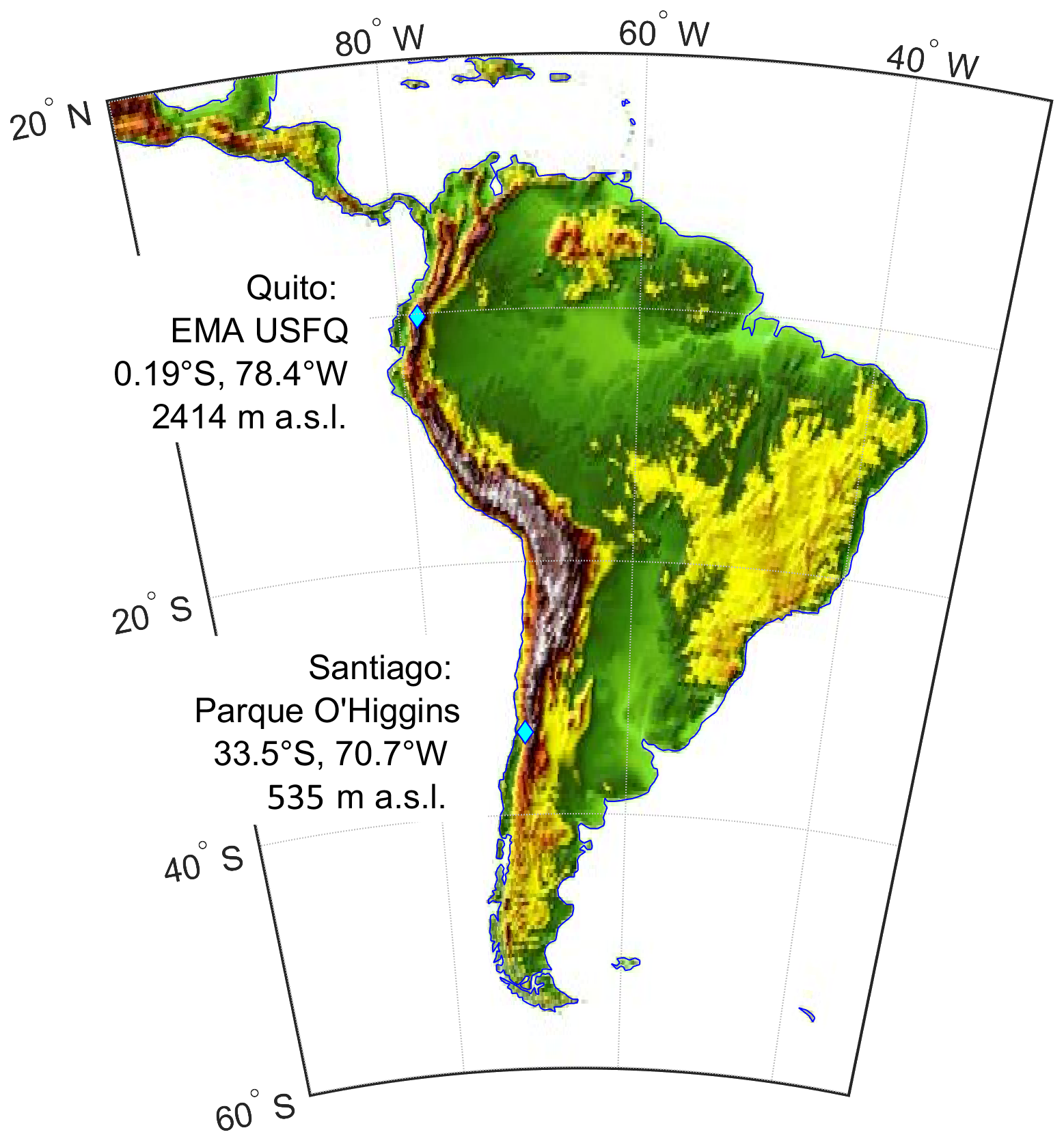
Figure 1 Map of South America with location and coordinates of EMA USFQ station in Quito, Ecuador, and Parque O'Higgins station in Santiago, Chile.

2.2 Study sites and background information

A map with the location of the two study sites in Quito, Ecuador, and Santiago, Chile is shown in Fig. 1. Details of the stations chosen for the study as well as background information follow.

One of the sites is located at Universidad San Francisco de Quito's Atmospheric Measurement Station (EMA USFQ, Spanish acronym) at coordinates 0.19° S, 78.43° W, and 2414 m a.s.l. Quito (2.78 million inhabitants) is an Andean city located at high altitude on the Equator. In Quito, the typical UV index is greater than 11 on 40.0 %–76.1 % of days per month, while the number of days per month with UV index greater than 16.0 varies between 0.7 % and 32.0 % (Parra et al., 2019). In particular, intense insolation and UV index take place during the equinox months of March and September. In parallel, the times of the year with increased precipitation peak around March–April and November, while the drier months run from July to September (Cazorla et al., 2024), although conditions vary mildly within a year. A discussion on weather patterns that influence air quality in Quito can be found in previous work (Cazorla and Juncosa, 2018).

In Santiago, we chose Parque O'Higgins station, located some 5 km away from downtown Santiago, at coordinates 33.46° S, 70.66° W, and 535 m a.s.l. This station is run by the Ministry of the Environment, and it typically represents the city's average conditions (Osses et al., 2013). Santiago (8 million inhabitants) is a subtropical city that exhibits four seasons. The warmest and sunniest months take place during the austral summer (December to February), but the high ozone season often extends until March. This is an interesting month in terms of air quality in Santiago because high temperatures and insolation prevail, while anthropogenic emissions and ozone precursors increase as the school year starts and the flow of people into the city increases.

2.3 Study time periods

2.3.1 Santiago

Ozone production was calculated for time periods in 2021 and 2022. A field campaign to measure VOCs in Santiago was conducted in March 2021 (description in Sect. 2.4.2 and Appendix A). Therefore, we performed detailed modeling of the chemistry of ozone production for sunny days during the month of March. We filtered out overcast days because photolysis frequencies were not measured and, thus, we rely on modeled actinic flux without cloud cover correction for the photolysis component of the model. March 2021 was mostly sunny in Santiago, so only 5 d were filtered out. Fig. S1 in the Supplement shows the time series of solar radiation overlapping mostly sunny days to all days.

To further explore ozone production under additional precursor conditions that are typically observed within a year, we ran simulations for average conditions per season in 2022. Thus, we run the model for a typical sunny day in austral summer (February and March, data in January was not included because of poor quality), fall (April, May), winter (June to August), and spring (September to November). As in the previous case, we filtered out overcast days from the time series. Mean conditions were found by overlapping meteorological and air quality data (1 h resolution) in 24 h plots and finding the average for every hour, namely the mean diurnal variation (MDV). These mean conditions were used as inputs to run the model. Model input variables are described in Sect. 3.

2.3.2 Quito

As in the case of Santiago, we performed detailed photochemical modeling for sunny days in March 2021 (11 overcast days were filtered out, Fig. S1) and for typical sunny conditions in 2022. Thus, we ran the model for typical conditions in January, often a sunny month; June–July, a time with low precursors due to summer vacation; September, an equinox month with increased precursors due to the return from summer vacation; and October–November, a time of transitioning into the rainy season. Mean conditions (sunny days only) for each period were found in a similar way as it was done for Santiago.

2.4 Data

2.4.1 Ozone, NO, NO₂, CO, and meteorological data

Santiago

Air quality data and meteorological conditions (1 h) measured at Parque O'Higgins station were obtained from the Air Quality National Information System maintained by the Ministry of Environment (SINCA, Spanish acronym, https://sinca.mma.gob.cl/, last access: 1 October 2024). From network information, ozone is measured with UV photometry, NO_x with chemiluminescence, CO with infrared photometry, and published data complies with quality control standards according to national legislation (https://sinca.mma.gob.cl/index.php/documentos, last access: 1 October 2024). Figure S2 in the Supplement depicts the time series of measurements in March 2021. For comparisons with Quito, the time coordinates in all figures in this work are presented in UTC−5 (local and solar time in Quito and roughly solar time in Santiago).

All data described in this section are available as complete input files for the F0AM model for Quito (Cazorla et al., 2025a) and Santiago (Cazorla et al., 2025b), see also the Data Availability statement.

Quito

Ozone is measured at EMA USFQ with a Thermo 49i UV photometer. Measurements are periodically intercompared against a 2B-Technologies UV photometer. The agreement between measurements is better than 5 %. A Teledyne 400 chemiluminescence instrument is used to measure NO-NO₂-NO_x. Calibration is done with a certified NO standard and zero air to prepare calibration mixtures. Uncertainty in measurements is better than 5 % (Cazorla, 2016). The original rate of acquisition of ozone and NO_x measurements is 1 s. Meteorological measurements are also available at EMA USFQ with an original rate of acquisition of 30 s. CO is not measured at EMA USFQ. However, the car fleet is similar in the entire city. Hence, following previous work (Cazorla et al., 2021), we used an average of CO measurements from three stations (Belisario, Centro and Tumbaco) run by the Quito Air Quality Network (Secretariat of the Environment, Quito, Ecuador) (https://aireambiente.quito.gob.ec/, last access: 15 August 2024). Figure S3 depicts the time series of Quito observations.

2.4.2 In situ measurements of VOCs in Santiago

VOC measurements in Santiago were taken from a fourth story window at the Geophysics Department of Universidad de Chile (33.457° S, 70.662° W, 535 m a.s.l.) from 17 to 28 March 2021, corresponding to the late summer. The site is located at campus Beauchef, in downtown Santiago, 770 m away from Parque O'Higgins station, where ozone, carbon monoxide, nitrogen oxides, and meteorological parameters are measured.

Table 1 VOCs measured in Santiago from 17 to 28 March 2021 and linear regressions of VOCs vs. CO in ppbv.

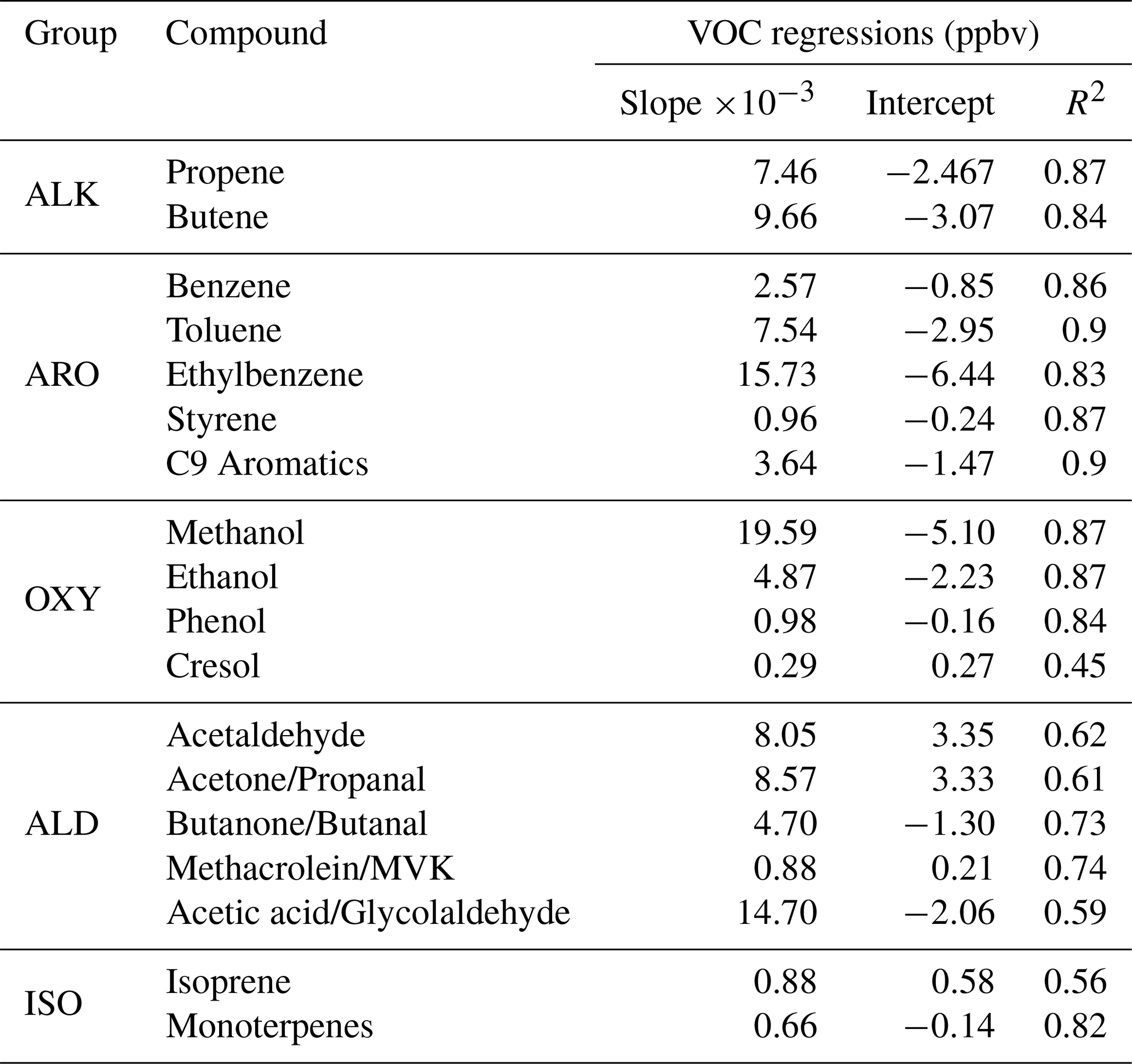
VOCs were measured using PTR-TOF-MS (proton transfer reaction time of flight mass spectrometry) at 1 s resolution. The instrument used was an Ionicon Analytik GmbH, Model 1000. A detailed description of the sampling operation of the PTR-TOF-MS instrument, calibration and mass discrimination methodology as well as the limit of detection of measured compounds is given in Appendix A. Table 1 shows the VOCs utilized in this study. Grouping was done for the practical purpose of organizing model runs, as explained in Sect. 2.5. The ISO nomenclature contains isoprene and monoterpenes also for practical reasons (isoprene contributes to P(O₃) formation but the monoterpene contribution was found to be marginal). In Appendix B (Fig. B1), we present the time series of measured VOCs. Based on details in Appendix A, we estimate a conservative error of 30 %–40 % in all VOC observations.

Previous studies conducted in numerous cities demonstrate that ambient measurements of VOCs, especially those whose source is fuel in vehicles, linearly correlate with CO, an anthropogenic tracer of combustion (Baker et al., 2008; Bon et al., 2011; Borbon et al., 2013; Brito et al., 2015). These correlations are useful as they can be used as emission ratios (Borbon et al., 2013). Thus, we obtained linear regressions between VOC and CO observations in Santiago for the campaign period. To this end, we linearly correlated the diurnal cycle of each VOC with the diurnal cycle of CO. We checked the results by correlating nighttime VOC and CO measurements and subtracting the background CO (noontime concentration) from the time series (Borbon et al., 2013; Brito et al., 2015). Both approaches yielded about similar slope values, but the determination coefficients were generally lower for the second approach. However, the determination coefficients improved for cresol, acetaldehyde, acetone, and isoprene. Thus, only for the latter compounds we used the linear fits obtained with the second approach. Table 1 shows the linear fit parameters used in this work. Table S1 contains the parameter regressions obtained with both approaches. Graphs for the VOC vs. CO regressions for benzene and toluene can be found in Figs. S4 and S5. The entire compendium of regression figures (both methods) can be found in the link indicated in the Data availability statement.

Compared to $\mathrm{VOC}/\mathrm{CO}$ ratios (slope of linear fit in pptv ppbv⁻¹) reported for other cities in Latin America, namely Mexico City (Bon et al., 2011) and São Paulo (Brito et al., 2015), the slope we found for benzene (2.57) is about twice the value reported for Mexico City (1.21) and 2.5 times the value for São Paulo (1.03). For toluene, the slope in this study (7.54) is also higher than in Mexico City (4.2) and São Paulo (3.1). For C9 aromatics, we found a value of 3.64, close to what was reported in Mexico City (2.8). The Mexico City and São Paulo studies were done about a decade ago. Further work is needed regionally to better compare these ratios across cities, preferably with more recent measurements.

Linear fits for compounds associated with traffic (10 cases) show R²>0.83 and correspond to alkenes, aromatics, and some oxygenated compounds (methanol, ethanol, and phenol). Some of the latter compounds could also have a biogenic origin, but finding exact proportions from each source was not within the scope of this study. The determination coefficient is less good for other oxygenated compounds, namely acetaldehyde, acetone, and acetic acid (R²∼0.61), which can be attributed to the secondary nature of these compounds. As expected, the linear fit for isoprene is less good (R²=0.56) due to its combined anthropogenic and biogenic origin. In contrast, monoterpenes correlate well (R²=0.82), for which we associate these compounds with traffic sources in addition to biogenic sources as observed in other cities (Borbon et al., 2023).

2.4.3 Monte Carlo perturbations on VOCs in Santiago

Direct measurements of VOCs were not available in Santiago on all days of March 2021 or on typical days per season in 2022. In addition, the available measurements were subject to methodological limitations, as previously discussed. Given the error in measurements and the uncertainty of applying regressions in Table 1 to derive VOCs at times other than the campaign period, we ran 10 000 Monte Carlo (MC) simulations within ±35 % of the known values to find an array of inputs to the F0AM model. Thus, we ran individual MC simulations for 22 compounds (Table 1). From the bulk of each MC simulation, we extracted percentiles 10 to 90, which covered the simulation range. Figure S6 depicts the flow diagram followed to generate MC simulations. In Fig. S7, we present the MC simulations for benzene (time series and percentile distribution as diurnal cycles). The entire compendium of MC simulation figures for all VOCs are accessible through the link provided under Data Availability.

2.4.4 Simulations of VOCs in Quito

Measurements of VOCs are unavailable in Quito. For this reason, we used a Monte Carlo approach to simulate VOCs and to find an array of inputs to the model. VOCs in Quito could be derived from CO provided suitable emission ratios were available (Borbon et al., 2013). Given the lack of experimental data, we generated VOCs using CO measurements in Quito and the regressions in Table 1. Subsequently, we perturbed these data 10 000 times within ±50 % through Monte Carlo simulations. This conservative factor was applied based on the observation that CO in Quito varies from CO in Santiago by about ±25 % at noon, but during rush hours this variability could be up to ±50 %. From the bulk of the simulations, we extracted percentiles 10 to 90. This process was applied to all time periods analyzed in this study. In Fig. S8, we present the flow diagram followed to generate VOCs.

In Quito, 98 % of ambient CO is a primary emission that comes from on-road traffic (Hernandez and Mendez, 2020; Parra, 2017; Vega et al., 2015). Hence, alkene and aromatic compounds such as propene, butene, benzene, toluene, and xylenes, as well as C8 and C9 aromatics, are expected in the Quito environment. Fuel options such as gasoline mixtures with ethanol are not currently commercialized in Quito, but they are available in some other cities, mainly in the coast of Ecuador. Thus, we included ethanol and methanol to investigate the potential effect if these types of fuels were available. In addition, methanol can also be present from biogenic sources. Aldehydes and ketones are usually present in an urban environment as they are byproducts of oxidation and photolysis reactions.

We present MC simulations for benzene in Fig. S9. The entire compendium of MC simulation figures for all VOCs for Quito can be found in the link provided under Data availability.

2.5 Model details

We used the F0AM (Wolfe et al., 2016) to model ozone formation chemistry in Quito and Santiago in the time periods indicated in Sect. 2.3. The chemical mechanistic information was taken from the Master Chemical Mechanism, MCM v3.3.1 (Bloss et al., 2005; Jenkin et al., 1997, 2003, 2015; Saunders et al., 2003), via website: http://www.mcm.york.ac.uk (last access: 1 July 2024). The F0AM is a model that runs in MATLAB (https://la.mathworks.com/, last access: 1 May 2024). Details of model settings and simulations follow.

2.5.1 Model input and options

Time step

The time step for the March 2021 model runs for Santiago and Quito was 10 min. To this end, the original Quito data were integrated into 10 min resolution. The same was done with Santiago 1 min VOC data. Regarding air quality and meteorological observations in Santiago, 1 h data were interpolated to generate 10 min time series. In contrast, the 2022 runs were done using 1 h data for average conditions in a season (Santiago) or month-grouping (Quito).

Model constraints, boundary layer depth, and dilution constant

We constrained the model with ozone, CO, and meteorological observations from both cities. VOCs (obtained as described in the previous section) were also used to constrain the model. NO and NO₂ were not constrained but the NO_x sum was conserved (constrained). Following model recommendations, background concentrations were set to zero to avoid buildup of secondary species (Wolfe, 2023).

For boundary layer depth (PBLh) we used results from previous work done in Quito and Santiago. For Quito, we used the empirical model published by Cazorla and Juncosa (2018) that was inferred from balloon-borne measurements of PBLh and surface observations between 2014 and 2017. This approach was used to obtain PBLh in March 2021 and for the 2022 runs. For Santiago, we used results from the EMEP MSC-W model, that is an offline chemical transport model (Simpson et al., 2012), as recently applied in Santiago and other South American cities (Pachón et al., 2024). For the seasonal runs in 2022, we scaled the March 2021 PBLh with an empirical factor using, as reference, previous work (Muñoz and Undurraga, 2010). Thus, we used $\mathrm{1}/\mathrm{3}$ of the summertime values for winter PBLh and $\mathrm{2}/\mathrm{3}$ for fall. Figure S10 shows PBLh for Quito and Santiago in March 2021.

As stated in the F0AM model documentation, dilution is treated as a first order sink (Wolfe, 2023). Thus, we calculated a first order constant of dilution (kdil in the model) for each city by relating the time evolution of the PBL (m s⁻¹) to PBLh (m) at every step of the run. The bottom panels in Fig. S10 show kdil for both cities.

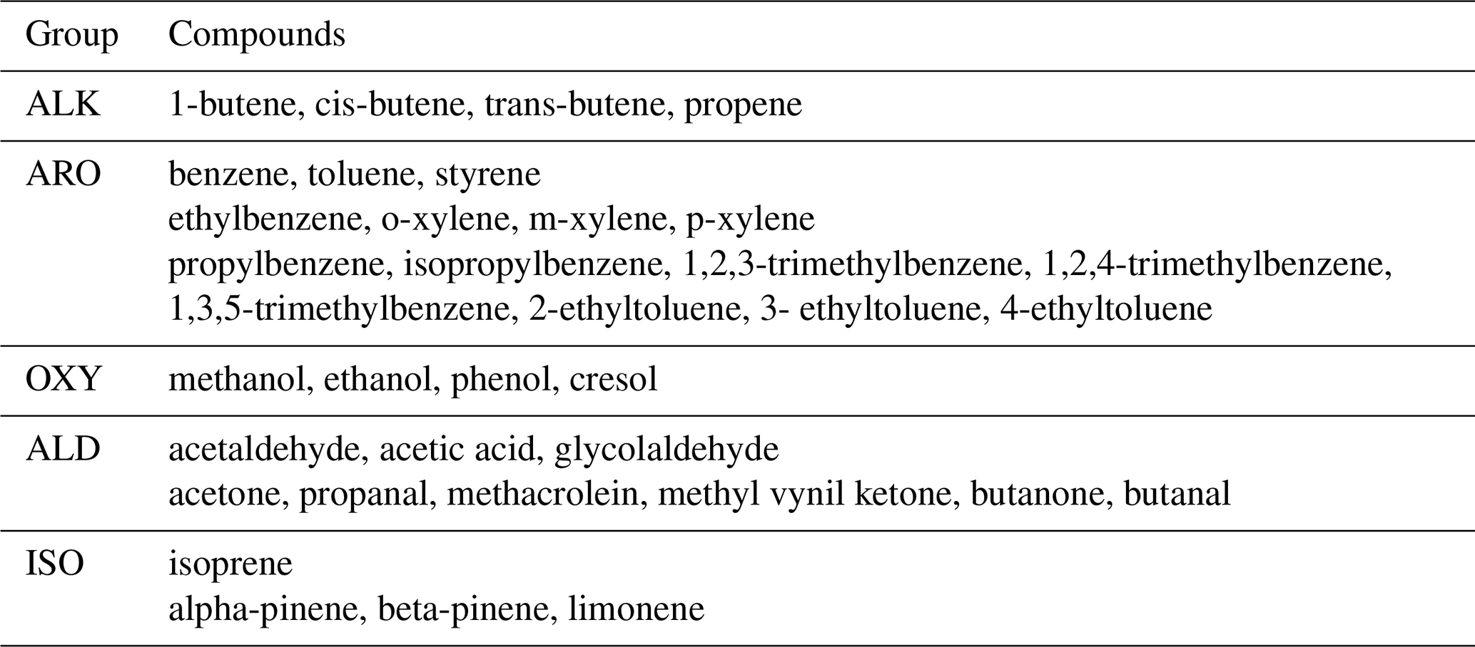
Table 2 VOCs measured in Santiago, Chile in March 2021 and used as model input.

VOC input

For the VOC input, compounds were distributed among explicit VOCs available in the MCM using weighing factors indicated in Table S2 in the Supplement. For example, compounds measured as butanone/butanal were distributed as 50 % butanone and 50 % butanal. These correspond to MCM notations MEK and C₃H₇CHO, respectively. Thus, a total of 36 VOCs were input to the model resulting in 9189 reactions. Compound-grouping and notation used in this study, along with all input species are depicted in Table 2.

Frequencies of photolysis ozone column and albedo

Frequencies of photolysis were modeled using the MCM option in the F0AM for both cities. In the Results section we compare the mean diurnal variation of JNO₂ and JO¹D between both cities and with previous studies. For the ozone column and albedo, we used 1 h area-averaged MERRA-2 (Modern-Era Retrospective analysis for Research and Applications, Version 2) data sets for Quito and Santiago (Global Modeling and Assimilation Office (GMAO), 2015a, b). This data selection was based on previous work that showed good performance of MERRA-2 products for total column ozone in the region (Cazorla and Herrera, 2022). Table S3 contains a summary of options chosen in the F0AM for model runs.

2.5.2 Sensitivity runs

We ran a series of experiments to investigate the individual contribution of VOC groups to P(O₃) as well as the sensitivity of P(O₃) to different combinations of VOC and NO_x levels.

For determining the contribution of VOC groups to P(O₃), we ran the model starting with alkenes (ALK) and adding one VOC group at the time until completion of all groups (ALK, ARO, OXY, ALD, and ISO). From these runs, we determined the percentage contribution of each group to P(O₃) in each city. For the last group (ISO), the percentage contribution refers to isoprene because adding monoterpenes essentially did not cause change.

We tested the sensitivity of P(O₃) to VOC levels P10, P50, and P90 (percentiles 10, 50 and 90 from MC simulations) under observed NO_x concentrations, 25 % NO_x reductions, and 75 % NO_x reductions in each city. VOC level P10 (P90) corresponds to a 30 % decrease (increase) from P50 in Santiago and 40 % in Quito. The group contribution runs were done using P50. In addition, we performed seasonal runs in 2022 for the entire VOC range (P10, P50, and P90) under observed NO_x levels in each city. Thus, we present the results from a total of 50 model runs (25 per city).

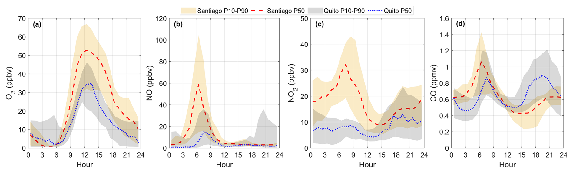
Figure 2 Diurnal variation of (a) ozone, (b) NO, (c) NO₂, and (d) CO observed in Santiago and Quito in March 2021. The red dashed line is the diurnal variation from observations in Santiago at the 50th percentile and the dotted blue line is the same but for Quito. The orange shadow is limited at the bottom and top by the 10th and 90th percentile diurnal variations from observations of every variable in Santiago. The gray shadow is the same but for Quito. Time is in UTC−5.

3 Results and discussion

3.1 March 2021

3.1.1 Air pollutant levels

Ozone maxima in Santiago ranged between 30 to below 70 ppbv in March 2021, as shown by percentiles 10 and 90 of diurnal profiles obtained with 1 h observations in Fig. 2a. Looking at the entire data set, half of the days in the month had ozone higher than 50 ppbv and there was a day with a maximum of 100 ppbv on 4 March (the school year started on 1 March). Unlike Santiago, Quito does not have a well-established ozone problem or season, despite equatorial solar radiation at high altitude and urban emissions. Usually, 1 h data remain below 50 ppbv. For example, in March 2021, ozone maxima during mostly sunny days ranged between 30 to 50 ppbv for percentiles 10 and 90 as depicted in Fig. 2a. In previous years, high ozone in Quito (up to 80 ppbv) has been recorded episodically and has been associated with wildfires in the surrounding forests, usually during the month of September (Cadena et al., 2021). During the study period, PM_2.5 levels (24 h mean) were 17.6 µg m⁻³ in Quito and 22 µg m⁻³ in Santiago.

Regarding levels of NO_x, ambient concentrations of NO and NO₂ in Santiago in March 2021 were greater than in Quito by a factor of 3 for the maximum at the 50th percentile, as depicted in Fig. 2b and c. However, levels of CO at the 50th percentile from the mid-morning to noon were about similar (Fig. 2d), although data dispersion is within ±25 %. During the rush hours CO can differ by ±50 %. The CO and NO diurnal profiles show strong traffic signatures in the morning and evening rush hours over Quito. In contrast, the morning rush hour in Santiago stands out more, while the evening signature is delayed and less prominent. These features are associated with the urban activity and work habits of citizens in both cities. In Santiago, work hours extend into the evening and night, often past the work schedule, and citizens take a long time to return to their homes. In Quito, citizens usually leave work before dark and usually do not extend the 8 h work schedule.

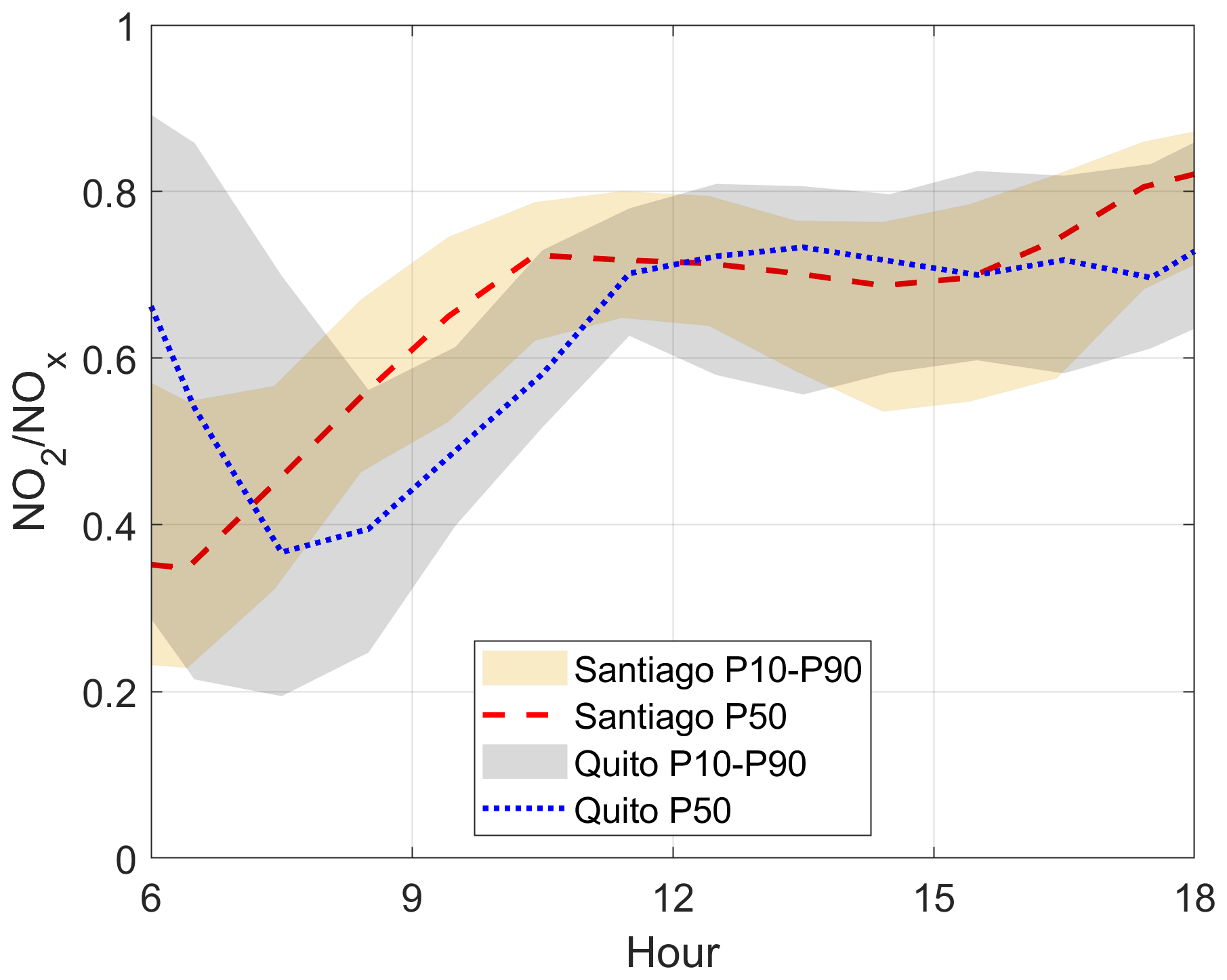
Figure 3 Diurnal variation of the ${\mathrm{NO}}_{\mathrm{2}}/{\mathrm{NO}}_x$ ratio at the 50th percentile from observations in Santiago (red dashed line) and Quito (blue dotted line) in March 2021. Shadows depict limits at the 10th and 90th percentiles at Santiago (orange) and Quito (gray). Time is in UTC−5.

The diurnal ${\mathrm{NO}}_{\mathrm{2}}/{\mathrm{NO}}_x$ ratio is an indicator of photochemical activity. It involves nitric oxide (NO) reacting with hydroperoxyl (HO₂) and alkyl peroxy (RO₂) radicals to form NO₂. The shape of the diurnal cycle of this ratio is similar between Quito and Santiago. However, Santiago's photochemical activity starts earlier than in Quito as given by an earlier increase of ${\mathrm{NO}}_{\mathrm{2}}/{\mathrm{NO}}_x$ (Fig. 3) right after the rush hour dip (due to increased NO_x from traffic emissions). This is related to the earlier start in traffic in Santiago as seen in NO and CO (Fig. 2b and d), which in turn leads to a distinct NO₂ morning maximum that is not present in Quito (Fig. 2c). At noon and in the afternoon, ${\mathrm{NO}}_{\mathrm{2}}/{\mathrm{NO}}_x$ at the 50th percentile (observations) is about similar in both cities, which indicates similar photochemical activity.

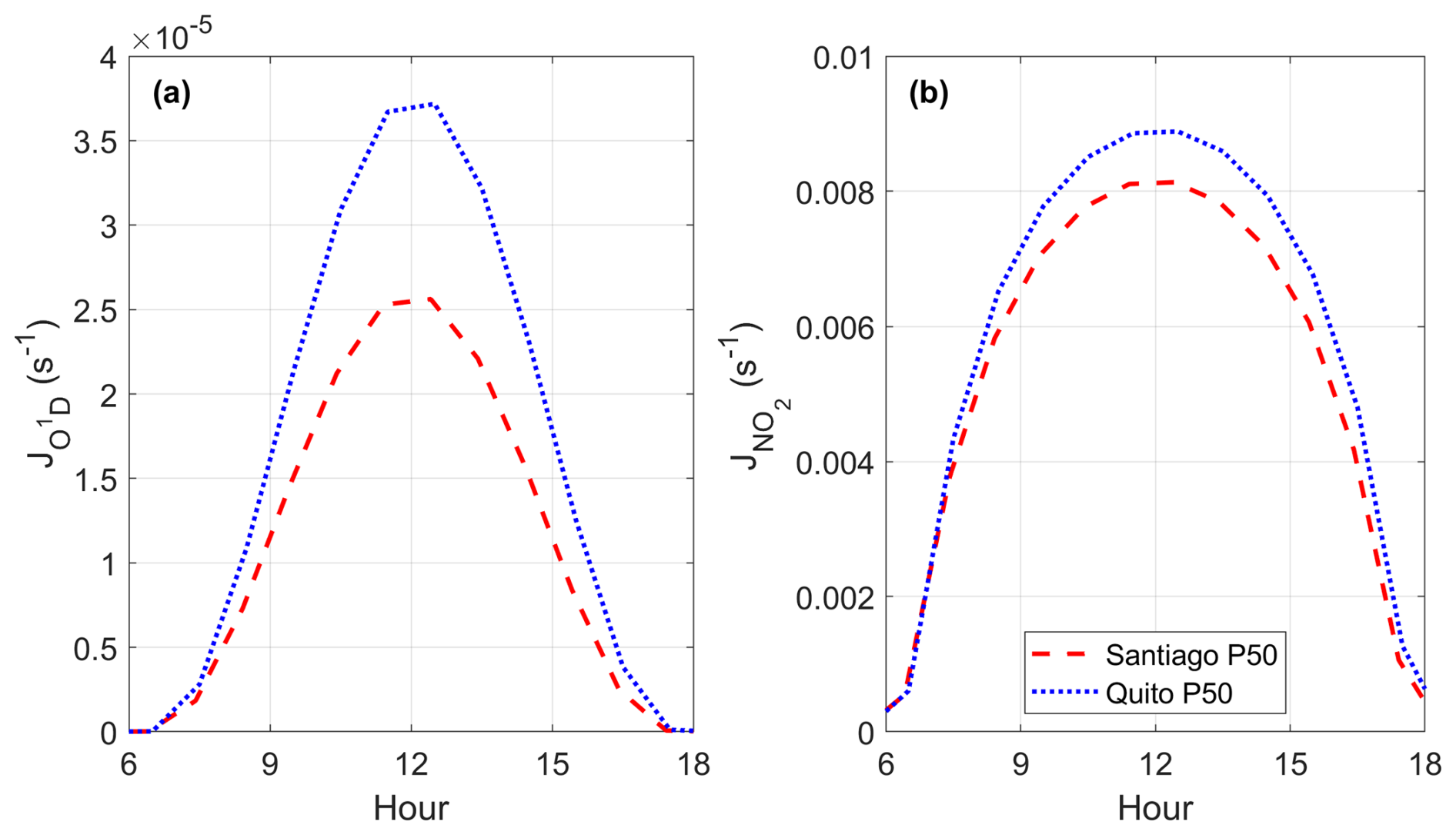
Figure 4 Comparison between the diurnal variation of frequencies of photolysis (a) JO¹D and (b) JNO₂ in Quito and Santiago at the 50th percentile from model output. Time is in UTC−5.

3.1.2 Model output

JO¹D and JNO₂

Photolysis reactions are key to radical and ozone production during daylight hours. Being that Quito and Santiago are located on the Equator and in the subtropics, respectively, the magnitude of frequencies of photolysis are different due to the intensity of solar radiation at both locations. From model output, the diurnal variation at the 50th percentile of frequencies of photolysis of ozone (towards the production of O¹D) and NO₂ in March 2021 are presented in Fig. 4. As expected, both quantities are greater in Quito than in Santiago due to its equatorial location and high altitude. Previous work on the oxidation capacity of the Santiago air reported direct measurements of JO¹D and JNO₂ taken during a field campaign in March 2005 (Elshorbany et al., 2009b). These measurements for diurnal maxima in Santiago were JNO₂∼0.008 and JO¹D $\sim \mathrm{2.5}\times {\mathrm{10}}^{-\mathrm{5}}$ s⁻¹, which are similar to mean values obtained through modeling in this work.

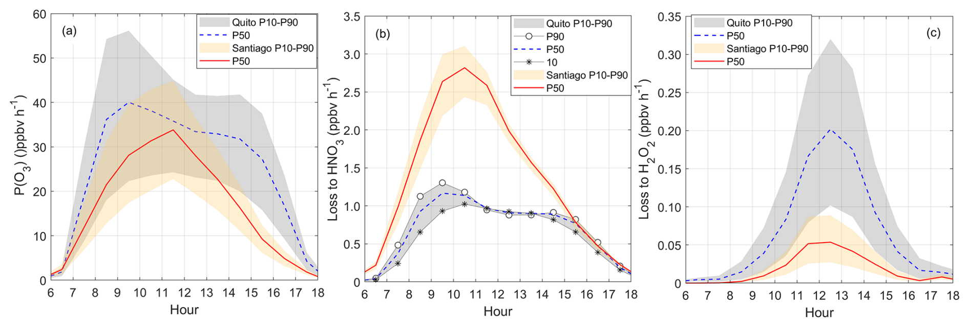
Figure 5 Diurnal variation of (a) net ozone production, (b) loss to nitric acid, and (c) loss to hydrogen peroxide in Quito and Santiago. Shadows correspond to boundaries obtained with VOC levels P10 (10th percentile) and P90 (90th percentile) from Monte Carlo simulations (orange for Santiago and gray for Quito). Symbols were added to better visualize percentile boundaries when needed. Results obtained at the VOC level P50 (50th percentile) are given by the solid red line for Santiago and dashed blue line for Quito in each graph. Time is in UTC−5.

Ozone production and loss

Ozone production rates were modeled for a range of VOC inputs and so are discussed in terms of ranges bounded by percentiles P10 and P90 obtained from the VOC distribution in each city (Fig. 5a). For Santiago, the range represents the uncertainty in the P(O₃) simulation given the uncertainty in VOC measurements. Thus, the best estimation of P(O₃) for Santiago is represented by P50 in Fig. 5a. The uncertainty was determined from the mean percentage difference of the upper and lower boundaries from percentile 50 and corresponds to ±32 % (Fig. S11). For Quito, P10 and P90 set the boundaries of the possible range of P(O₃) magnitudes expected for Quito calculated to the best of our knowledge from a distribution of VOC inputs. Due to a lack of in situ measurements we deal with the entire range when discussing Quito and we only present P50 curves in a referential way. The mean variability from percentile 50 is ±42 % (Fig. S11).

The range of net ozone production rates at both cities at noon are comparable (22–45 ppbv h⁻¹), but in the mid-morning values could be higher for the upper boundary in Quito (up to 55 ppbv h⁻¹) (Fig. 5a). Further below we show that in Quito the HO₂ and RO₂ abundance is greater when compared to Santiago (Fig. 9), but NO levels are lower (Fig. 2b). Thus, there is a compensating effect in the levels of HO₂ and NO in both cities in a way that application of Eq. (1) yields about similar ozone production rates. Previous work that determined net ozone production rates in Santiago from measurements and model calculations in 2005, reported substantially higher values for the mean P(O₃) diurnal maximum (160 ppbv h⁻¹) (Elshorbany et al., 2009a). Such high value is outside of our calculation range, although it is possible that after almost 20 years of reassessing P(O₃) in Santiago, conditions changed. P(O₃) maxima presented in Fig. 5a for percentiles 50 of the distributions in both cities are consistent with values obtained in previous studies. For example, direct measurements of P(O₃) in Houston in 2009 were about 30 ppbv h⁻¹ on average (Cazorla et al., 2012). Another example is a recent sensitivity study of ozone production to NO_x and VOCs in New York city that found P(O₃) within 26–37 ppbv h⁻¹ from modeling work with the F0AM (Sebol et al., 2024).

Losses to nitric acid are higher in Santiago than in Quito (Fig. 5b). This is consistent with higher NO_x levels present in the Santiago ambient air. Meanwhile, losses to hydrogen peroxide are higher in Quito but the magnitude of this loss is one order of magnitude lower that the loss to nitric acid (Fig. 5c). Other losses are presented in Fig. S12. The loss due to ozone photolysis and the reaction of ozone with HO₂ are two and one orders of magnitude lower than the loss to nitric acid, respectively. The reaction of ozone with alkenes is also an order of magnitude lower than the loss to nitric acid, but this is higher than the loss to hydrogen peroxide. The upper boundaries of the loss to alkyl nitrates (P(RONO₂)) approach a digit and become important along with the loss to nitric acid in both cities.

NO and NO₂ were unconstrained in the model, but the NO_x sum was constrained. A comparison of measured and modeled $\mathrm{NO}/{\mathrm{NO}}_{\mathrm{2}}$ ratio is presented in Fig. S13. From the mid-morning to the early afternoon values are about similar.

An interesting point to investigate in the future is the connection between ozone production rates and ambient ozone, whose budget not only depends on atmospheric chemistry but also on meteorological and circulation factors, including long-range transport. From our calculations, the range of P(O₃) in both cities is similar but ambient ozone is higher in Santiago. This city has a year-round influence of the Subtropical Pacific High that determines a strong subsidence inversion, which is often strengthened by low-level lows and occasionally disrupted by passing synoptic disturbances (Gallardo et al., 2002; Garreaud et al., 2002; Huneeus et al., 2006; Muñoz and Undurraga, 2010). Such meteorological condition is known to be the cause of pollutant accumulation in the boundary layer in Santiago. In contrast, Quito is not affected by a similar high-pressure system. In our simulations, we used information of the boundary layer evolution in both cities. The boundary layer in Quito can often grow up to 2200 m a.g.l. (Fig. S10) (Cazorla and Juncosa, 2018). Under such conditions, the first order dilution constant in the model reached up to $\mathrm{2.5}\times {\mathrm{10}}^{-\mathrm{4}}$–$\mathrm{5.8}\times {\mathrm{10}}^{-\mathrm{4}}$ s⁻¹. Meanwhile in Santiago, the boundary layer can reach up to 1500 m and dilution constants usually stay below $\mathrm{2.5}\times {\mathrm{10}}^{-\mathrm{4}}$ s⁻¹ (Fig. S10). Additional research that uses a chemical transport model is needed to explain ambient ozone levels.

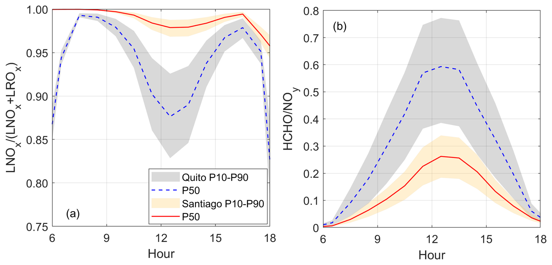
Figure 6 Indicators of the chemical regime of ozone production: (a) ratio ${\mathrm{LNO}}_x/({\mathrm{LNO}}_x+{\mathrm{LRO}}_x)$ (defined by Eqs. 3 and 4) and (b) ratio $\mathrm{HCHO}/{\mathrm{NO}}_y$ (formaldehyde to reactive nitrogen). Shaded area indicates model output boundaries obtained with the 10th and 90th percentiles (P10 and P90) of the VOC Monte Carlo distribution (orange for Santiago and gray for Quito). The solid red line and dashed blue lines correspond to model output at the 50th percentile (P50) for Santiago and Quito, respectively. Time is in UTC−5.

Ozone production regime

The chemical regime of ozone production in Santiago is strongly VOC-limited as indicated by the ratio ${\mathrm{LNO}}_x/({\mathrm{LNO}}_x+{\mathrm{LRO}}_x)$ being very close to one for the entire range of the model output as depicted in Fig. 6a. This indicator is consistent with the formaldehyde to reactive nitrogen ratio ($\mathrm{HCHO}/{\mathrm{NO}}_y$) being well below 1 (Fig. 6b), and with the losses to nitric acid being substantial (Fig. 5b).

For the Quito runs, ${\mathrm{LNO}}_x/({\mathrm{LNO}}_x+{\mathrm{LRO}}_x)$ points to a VOC-limited regime as this indicator is above suggested thresholds of 0.5 (Kleinman, 2005c; Kleinman et al., 2001) or revisited 0.74 (Schroeder et al., 2017). Meanwhile, the $\mathrm{HCHO}/{\mathrm{NO}}_y$ ratio is still below 1 for the entire range (VOC-limited) even though the upper boundary approaches one digit. This indicates that with a higher VOC content, the Quito environment is more prone to transitioning towards a more NO_x-limited regime. At the moment, a lack of in situ measurements constrains our ability to define how close the Quito environment is from the transition region. Even though from our calculations both cities are in the VOC-limited chemical regime, this character is noticeably more intense in Santiago from the indicators in Fig. 6. This finding illustrates that within the VOC-limited and NO_x-limited categories of ozone production there is a range of intensities that depend on the unique conditions that surround every urban area.

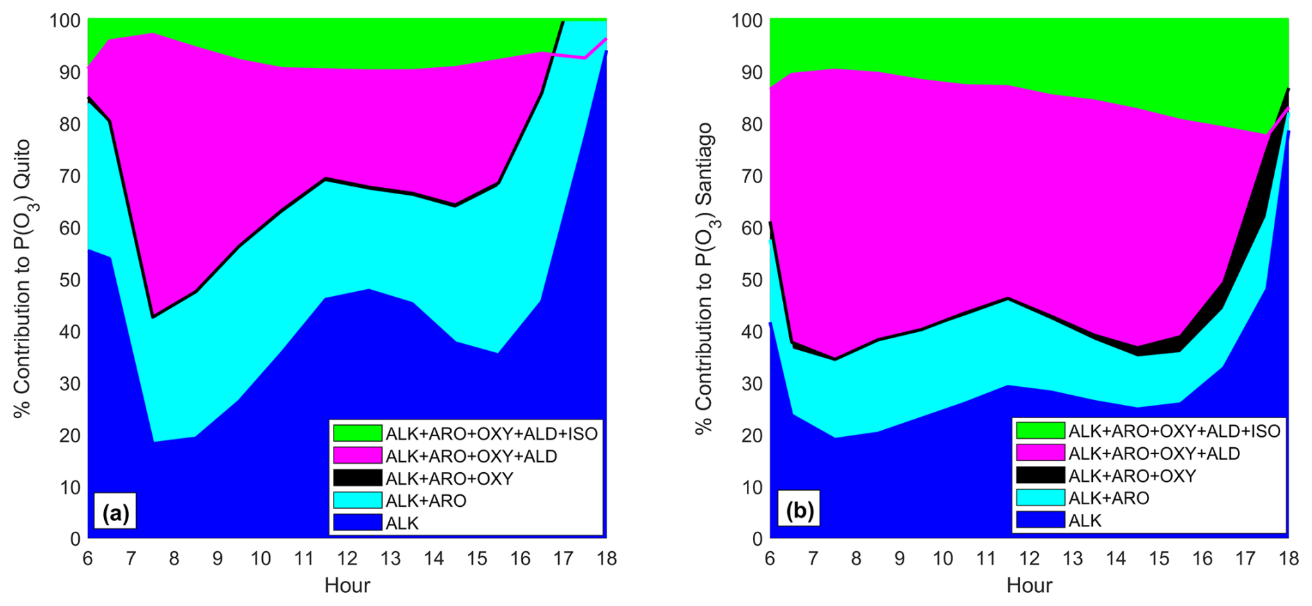
Figure 7 Percentage contribution to P(O₃) by chemical groups in (a) Quito and (b) Santiago obtained with model output at the 50th percentile from VOC Monte Carlo simulations. Time is in UTC−5.

VOC group contribution to P(O₃)

The percentage contribution to P(O₃) caused by every chemical group (Table 2) during daylight hours in both cities is depicted in Fig. 7a (Quito) and 7b (Santiago). For the Quito simulations, alkenes and aromatics combined (blue and cyan in Fig. 7a) contribute 45 % of ozone formation around the morning rush-hour, 70 % at noon, and up to 90 % in the afternoon. Meanwhile, the contribution of these two groups to P(O₃) in Santiago is under 50 % throughout the day. The contribution of aldehydes and ketones is substantial over Santiago and, when combined with alkenes and aromatics, adds up to 80 %–90 % of P(O₃) during daylight hours (magenta in Fig. 7b). In Quito, aldehydes and ketones are important in the morning, between 07:00–08:00, when the percentage contribution could be up to an additional 40 %–50 %, while at noon and in the afternoon this contribution is about 20 %. Isoprene contributes an additional 10 %–20 % in Santiago and becomes increasingly important towards the afternoon. In Quito, we estimate that this contribution is about 10 %. It must be noted that Central and Southern Chile suffered a long-standing drought between 2010 and 2022 (Garreaud et al., 2020) that likely caused an increase in isoprene emissions by vegetation due to hydrological stress (Jiang et al., 2018). The contribution of oxygenated compounds in both cities is marginal (black in Fig. 7). Future work needs to evaluate the contribution of alkanes in both cities as liquid petroleum gas is used for heating and cooking (Chen et al., 2001).

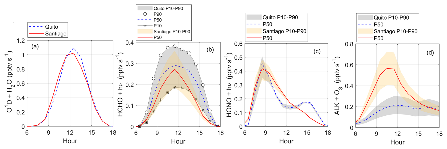
Figure 8 Diurnal variation of radical sources in Quito and Santiago: (a) ozone photolysis followed by O¹D + H₂O, (b) formaldehyde photolysis, (c) HONO photolysis, and (d) ozone reaction with alkenes. Shaded area indicates model output boundaries obtained with the 10th and 90th percentiles (P10 and P90) of the VOC Monte Carlo distribution (orange for Santiago and gray for Quito). Symbols were added to better visualize percentile boundaries when needed. The solid red line and dashed blue lines correspond to percentile 50 (P50) for Santiago and Quito, respectively. Time is in UTC−5.

Radical production and abundance

The main sources of radical production are depicted in Fig. 8 and correspond to the photolysis of ozone followed by the reaction of O¹D with water vapor (Fig. 8a), the photolysis of formaldehyde (Fig. 8b), the photolysis of HONO (Fig. 8c), and the reaction of ozone with alkenes (Fig. 8d). The first contribution has the largest magnitude in both cities. Computing this rate does not depend on VOC abundance for which percentile boundaries are absent in Fig. 8a. Thus, the curves depict the mean diurnal cycles whose maxima are about 1 pptv s⁻¹ in both cities, on average. However, within the month, variability in Santiago (0.5–1.75 pptv s⁻¹) is somewhat greater than in Quito (0.75–1.5 pptv s⁻¹). From meteorological data, the water vapor content at solar noon in Quito and Santiago is similar (10 vs. 9 g kg⁻¹) but solar radiation does not vary much on the Equator while in Santiago daylight progressively lowers as the season advances towards the fall.

P(HO_x) production from formaldehyde photolysis in Quito and Santiago is comparable (0.18–0.35 pptv s⁻¹) (Fig. 8b). Overall, this contribution is 2–3 times lower than the first source. In the morning, radical production from the photolysis of HONO is equally important in Santiago and in Quito (0.35–0.5 pptv s⁻¹), as indicated in Fig. 8c, which is expected given the high abundance of NO_x in the morning. However, the contribution from this radical source gradually decreases from the mid-morning into the afternoon. The contribution from the reaction of alkenes and ozone is higher in Santiago (Fig. 8d), which is consistent with higher ozone levels. Previous work determined P(HO_x) from different sources in Santiago (Elshorbany et al., 2009b). They found rates of HO₂ production from formaldehyde photolysis of 0.15 ppt s⁻¹, on average, and rates of OH production from HONO photolysis of 0.4 ppt s⁻¹. Our calculations are consistent with these findings. However, rates of OH production reported by Elshorbany et al. (2009b) from ozone photolysis are substantially lower (0.27 ppt s⁻¹, on average). It is important to remark that this study only considers gas phase chemistry and urban emissions following previous work (Elshorbany et al., 2009a, b; Ren, 2003; Ren et al., 2013).

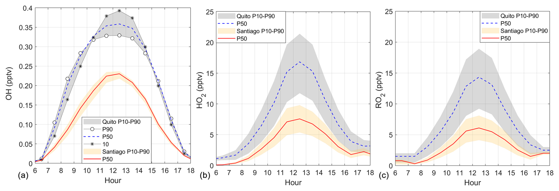
Figure 9 Diurnal variation of (a) OH, (b) HO₂, and (c) RO₂ in Quito and Santiago. Shaded area indicates model output boundaries obtained with the 10th and 90th percentiles (P10 and P90) of the VOC Monte Carlo distribution (orange for Santiago and gray for Quito). Symbols were added to better visualize percentile boundaries when needed. The solid red line and dashed blue lines correspond to the output with the VOC 50th percentile (P50) for Santiago and Quito, respectively. Time is in UTC−5.

Radical abundances in both cities during the study time period are illustrated in Fig. 9. With higher frequencies of photolysis, the OH abundance in Quito for the entire simulation range (0.33–0.38 pptv) is overall greater than in Santiago (0.23 pptv) (Fig. 9a). The order of magnitude of radical abundances is similar to those found in other studies (Cazorla et al., 2021; Dusanter et al., 2009; Ren et al., 2013). Given the greater OH availability in Quito, reactions with VOCs yield HO₂ and RO₂ abundances that at noon in Quito are about three times greater than in Santiago (Fig. 9b and c). From the magnitudes in the latter figures, HO₂ and RO₂ are equally important, which is consistent with previous work (Bottorff et al., 2023; Dusanter et al., 2009; Elshorbany et al., 2009b).

3.1.3 NO_x and VOC scenarios

In this section we explore the effect on P(O₃) due to changes in NO_x and VOCs that could arise from potential actions intended to improve air quality and help reduce SLCF. As stated before, diesel-based public transportation in South American cities is an important source of PM_2.5 and NO_x. It follows that a relevant scenario to consider is the effect on ozone production if this type of transportation were replaced, as it is often included in air quality and climate mitigation planning. Notice that Santiago's public transport bus fleet is roughly 10 % electric buses, a fraction that is expected to increase in the future. This type of action would significantly lower ambient NO_x (and PM_2.5), although VOCs would also decrease. Another relevant scenario is exploring changes in VOCs. For example, applying changes in the quality of fuels to reduce the content of aromatic compounds would influence P(O₃). Here, we explore some sensitivity scenarios, but additional research is needed to precisely determine the proportion in precursor reduction associated with specific environmental actions.

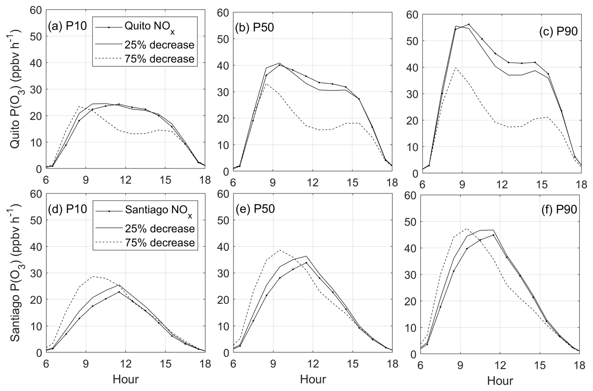
Figure 10 P(O₃) sensitivity to changes in NO_x and VOCs in Quito (a–c) and Santiago (d–f) obtained with VOC levels P10, P50 and P90 from Monte Carlo simulations. Time is in UTC−5.

The effect on P(O₃) with different combinations of NO_x and VOCs is quantified in Fig. 10. The scenarios investigated were those of current NO_x levels, NO_x reductions by 25 %, and NO_x reductions by 75 % at VOC levels P10, P50 and P90. For the latter, the percentage decrease (or increase) from P50 to P10 (or to P90) is 30 % in Santiago and 40 % in Quito. In Santiago and Quito, lowering the levels of VOCs would result in lower ozone production rates at all tested levels of NO_x as presented by the progression of panels in Fig. 10a to c (Quito) and 10d to f (Santiago). This feature is expected in VOC-limited environments. For example, at the current NO_x Quito levels, reducing VOCs by 40 % from the P50 level reduces the maximum P(O₃) by 37 %. In Santiago, a 30 % decrease in VOCs would result in a 32 % decrease in the maximum P(O₃).

At lower levels of VOCs in Quito (P10), a 25 % decrease in NO_x causes a slight P(O₃) increase in the morning and almost no change in the afternoon (Fig. 10a), while a 75 % NO_x reduction modestly raises the morning P(O₃) but causes a drop at noon. As VOC levels increase (P50 and P90), a 25 % reduction in NO_x causes a modest decrease in P(O₃), but a 75 % decrease causes the noon P(O₃) to decrease by half. This result indicates that at higher VOC levels in Quito the ozone production chemistry is prone to transitioning towards a more NO_x-limited regime, especially at noon and in the afternoon. This aspect underscores the necessity of implementing in situ measurements of VOCs in Quito to accurately determine how close the Quito environment is to the transition region.

In Santiago, at the current levels of VOCs and NO_x (P50), lowering NO_x increases ozone production rates, especially in the morning and mainly when the decrease is substantial (75 %), but the change at noon and in the afternoon is modest. Thus, at 09:00 a.m. P(O₃) grows from 25 to 38 ppbv h⁻¹ (Fig. 10e). Similar effects are observed at the lowest (P10) and highest (P90) VOC levels (Fig. 10d and f). Thus, P(O₃) increases in the morning and either there is a modest change or a decrease from noon to the afternoon. Therefore, NO_x decreases cause the peak P(O₃) to shift from noon to morning.

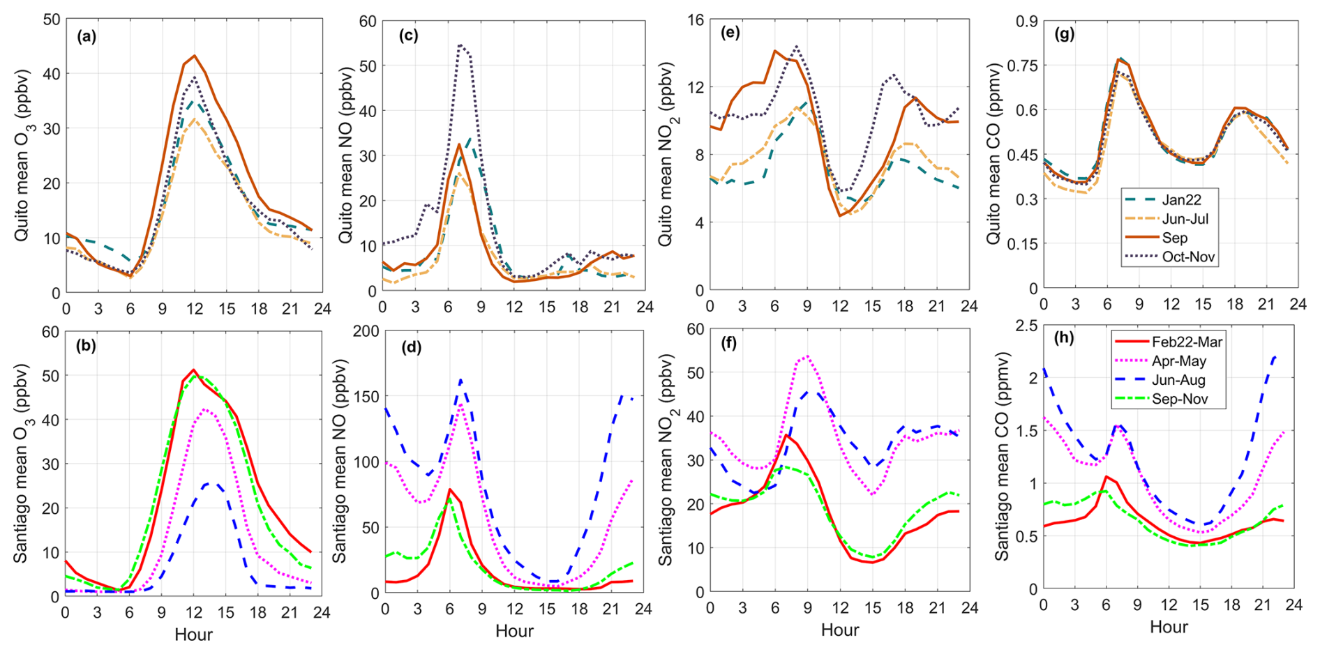
Figure 11 Mean air quality conditions observed within a year by season (Santiago) or month-grouping (Quito) presented comparatively for (a, b) ozone, (c, d) NO, (e, f) NO₂, and (g, h) CO. Time is in UTC−5.

3.2 Mean conditions by season in 2022

As per additional conditions observed within a year in Quito and Santiago, Fig. 11 illustrates the range of mean levels of O₃, NO, NO₂, and CO that are typically observed in both cities (2022 1 h data). In Quito, the daily ozone maxima range from 30 to 45 ppbv, with higher ozone in September and lower in June–July (Fig. 11a). In contrast, Santiago data show clear seasonal differences in data distribution with mean summer peak ozone concentrations being more than 2.5 times higher than those of the winter (20 vs. 55 ppbv) (Fig. 11b). The diurnal cycles shown in Fig. 11 are smoothed out when hourly data are averaged within a season. However, when inspecting the 1 h time series in Quito, only on 1 d in 2022 ozone was higher than 60 ppbv. Meanwhile in Santiago, the peak ozone values were between 60–100 ppbv in 48 d. Table S4 shows statistics for 2022 data in both places.

Regarding NO, peak values in the diurnal cycle in Quito range between 30 to 55 ppbv, but there are times in the year when NO spikes substantially during the rush hour (Fig. 11c). In 2022, this spike happened in October–November. In Santiago, NO is substantially higher in the winter months, when in addition to transportation and industry, residential sources become significant (Fig. 11d). As temperatures are low, the mixing volume remains shallow and primary pollutants such as NO accumulate, while the actinic flux is not sufficient to activate photochemistry. In the 1 h time series, 148 d in 2022 had NO higher than 100 ppbv in Santiago, while in Quito there were 31 d with morning NO of such magnitudes.

In Santiago, the winter-to-summer variability is also evident in the diurnal cycles of NO₂ and CO, with higher concentrations during the cold months (Fig. 11f and h). In contrast, the variability is small in Quito for NO₂, especially during daylight hours, and marginal for CO (Fig. 11e and g).

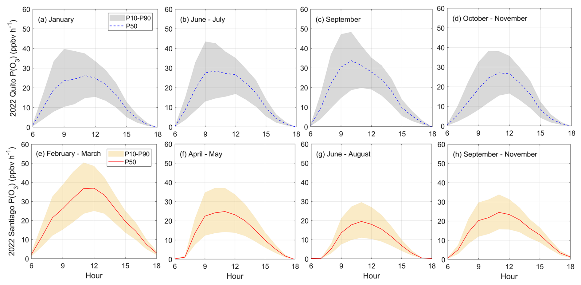
Figure 12 Comparison of the range of net ozone production rates observed in a year (2022) in Quito (a–d) and Santiago (e–h). Shaded area indicates model output boundaries obtained with the 10th and 90th percentiles (P10 and P90) of the VOC Monte Carlo distribution (orange for Santiago and gray for Quito). The solid red lines and dashed blue lines correspond to percentile 50 (P50) for Santiago and Quito, respectively. Time is in UTC−5.

With the range of conditions presented in Fig. 11, the range of ozone production rates calculated on average is depicted in the top panels of Fig. 12 for Quito and at the bottom for Santiago. In Quito, the mean ozone production rates roughly range from 15–40 ppbv h⁻¹ year-round (Fig. 12a to d), although in September the upper boundary is right under 50 ppbv h⁻¹. These magnitudes of P(O₃) resemble ozone production rates during the ozone season in Santiago (February–March, Fig. 12e). The rest of the seasons, P(O₃) in Santiago is lower by 10-20 ppbv h⁻¹. Therefore, with the range of VOCs used in the model, ozone production rates during sunny days in Quito stay high most of the year. In contrast, ozone in Santiago is high only during the ozone season. However, ozone levels in Quito are generally lower than in Santiago.

4 Conclusions

Ozone production rates in Quito and Santiago (sunny days) were calculated using the F0AM (Framework for 0-D Atmospheric Modeling) for March 2021 and for mean conditions per season in 2022. The model was constrained with ground station observations (air quality and meteorology) and VOCs. The latter were measured in Santiago during part of March 2021. When measurements were not available, VOCs were generated with experimental VOC vs. CO linear regressions and Monte Carlo simulations within 35 % of error in the observed values. We estimate an uncertainty of 32 % in P(O₃) calculations for Santiago. As measurements of VOCs in Quito are not available, we simulated the entire set of VOCs. To this end, we scaled Quito CO using Santiago linear regressions, but we perturbed these values within 50 % using Monte Carlo simulations. The percentage variability in the range of calculated P(O₃) for Quito is 42 % from the mean.

Santiago is impacted by a well-established ozone season during the austral summer, which extends into March. In March 2021, the P(O₃) maximum was 32 ppbv h⁻¹ (±32 % or 22–42 ppbv h⁻¹). During this period, there were 11 d in Santiago when 1 h ozone observations were between 60–80 ppbv and 1 d when ozone was 100 ppbv. In the summer 2022, the peak P(O₃) was similar (37 ppbv h⁻¹ ±32 %), while the rest of the seasons P(O₃) was 10–20 ppbv h⁻¹ lower. Meanwhile in Quito, our calculations indicate that the P(O₃) range in March 2021 was 23–45 ppbv h⁻¹ at noon, but in the mid-morning the upper boundary could reach 55 ppbv h⁻¹. From calculations in 2022 we found a range between 15–40 ppbv h⁻¹ except in September when the upper boundary could reach 50 ppbv h⁻¹. However, ozone levels in Quito (1 h) usually remain below 50 ppbv (only 1 d in 2022 was just over 60 ppbv). Therefore, we found that P(O₃) in Quito is comparable or possibly even higher than in Santiago (during the ozone season), but ambient ozone is generally lower. The air quality in Santiago is permanently impacted by the Subtropical Pacific High, which causes a strong subsidence inversion. In contrast, Quito is not influenced by a similar high-pressure system. Furthermore, we found that often a deep boundary layer of up to 2200 m develops over Quito and the model first order dilution constant reaches $\mathrm{2.5}\times {\mathrm{10}}^{-\mathrm{4}}$–$\mathrm{5.8}\times {\mathrm{10}}^{-\mathrm{4}}$ s⁻¹. Meanwhile in Santiago, we found that the boundary layer depth reaches 1500 m and the dilution constant stays below $\mathrm{2.5}\times {\mathrm{10}}^{-\mathrm{4}}$ s⁻¹. These findings provide some indications of relevant physical factors but additional research using a chemical transport model is needed to explain ambient ozone levels and the ozone budget.

As per the chemical nature of VOCs that contribute the most to the formation of ozone, we found that alkenes in Quito contribute 45 % in the morning and 70 %–90 % at noon and in the afternoon. In Santiago, the contribution of alkenes and aromatics is about 50 % throughout the day. Aldehydes and ketones contribute about 50 % in the morning in Quito and 20 % at noon and in the afternoon. In Santiago, aldehydes and ketones contribute an additional 40 %, which adds up to 90 % of the contribution along with alkenes and aromatics. We estimate that isoprene contributes about 10 % in Quito and 20 % in Santiago. The latter may be linked to the effects of a long-standing drought that affected Central and Southern Chile until 2022.

Ozone production rates of similar ranges in both cities result from a compensating effect in the magnitude of radical abundance relative to NO abundance. Thus, HO₂ and RO₂ radicals in Quito (HO₂: 12–22 pptv, RO₂: 9–18 pptv) are about twice the abundance in Santiago (HO₂: 6–9 pptv, RO₂: 4–8 pptv) but NO is two to three times higher in Santiago than in Quito. As in the case of ozone production rates, radical production rates from several sources are comparable in both cities. From ozone photolysis radical production rates are about 1 pptv s⁻¹; from formaldehyde photolysis 0.18–0.35 pptv s⁻¹; and from HONO photolysis 0.35–0.5 pptv s⁻¹. The contribution of ozone reactions with alkenes is greater in Santiago (0.4–0.7 pptv s⁻¹) than in Quito (0.12–0.3 pptv s⁻¹).

Indicators of the chemical regime of ozone production from model output, $({\mathrm{LNO}}_x/({\mathrm{LNO}}_x+{\mathrm{LRO}}_x$ and $\mathrm{HCHO}/{\mathrm{NO}}_y$), point to Santiago being a strongly VOC-limited environment. This is confirmed by higher ozone losses to nitric acid than in Quito although losses to the production of organic nitrate are comparable in both cities. In addition, from sensitivity tests in Santiago, NO_x reductions at all levels of VOCs lead to higher ozone production rates in the morning. In Quito, the two indicators also point to a chemical regime limited by VOCs. However, the value of $\mathrm{HCHO}/{\mathrm{NO}}_y$ (0.8) approaches 1 at higher percentiles of VOC abundance. At such VOC levels, NO_x decreases cause a drop in ozone production especially at noon and in the afternoon, which indicates transitioning into a more NO_x-limited regime. However, a lack of VOC measurements in Quito limits our ability to better determine these thresholds. From sensitivity tests, VOC reductions lead to a general decrease in P(O₃) in both cities.

Finally, our results remark the importance of implementing in situ measurements of VOCs in Quito and conducting more extended measurements in Santiago given the current conditions of environmental vulnerability and the need to implement policies that protect public health and climate.

Appendix A: VOC measurements in Santiago, Chile

VOCs were measured by a PTR-TOF-MS (Ionicon Analytik GmbH, Model 1000). Ambient air was drawn with an external pump (KNF, N86KN.18) through a sampling line ($\mathrm{1}/{\mathrm{8}}^{\prime \prime }$). The sample air was injected into the PTR from a T-union via a polyether-ether-ketone (PEEK) capillary ($\mathrm{1}/{\mathrm{16}}^{\prime \prime }$) conditioned at 80 °C. The ion source was supplied with a 15 cm³ min⁻¹ water vapor flow. The drift tube was operated at temperature, voltage and pressure of 353 K, 600 V and 2.3 mbar, respectively, corresponding to a reduced electric field strength ($E/N$ ratio) of ∼136 Td (Townsend) (1 Td = 10–17 V cm²).

The mass scale was calibrated every 10 min using H₃O⁺ isotope (21.0220), NO⁺ (29.9970) and protonated acetone (59.0490), while the voltage of the multichannel plate detector was optimized weekly. The relative mass discrimination (transmission) was calculated before the campaign using the sensitivity and known reaction rates. The limit of detection (LoD) was calculated as three times the standard deviation of the background signal from zero air measurements (ENVEA, Model ZAG7001). We use a certified gas standard (Airgas Specialty Gases) valid until 2023, traceable to NIST (National Institute of Standards and Technology), for calibration checks for benzene (79.054), toluene (93.070), and ethylbenzene + xylenes (107.086). The error for toluene, ethylbenzene + xylenes and benzene was −1.2 %, −34.6 % and +27.2 %, respectively.

PTR-TOF-MS provides several advantages, including mass range and high measurement frequency. However, this technique is susceptible to fragmentation that may interfere at a given $m/z$. The data used in this work resulted from a series of field campaigns aiming to optimize the measurements (e.g., $E/N$) and know the impact of fragmentation on benzene. We used specific ion peaks in the mass spectrum collected by Pagonis et al. (2019) in a public online library to identify reasonable VOC candidates in urban environments. Table A1 shows the protonated parent molecules detected in Santiago's atmosphere and the compound assigned by the monoisotopic $m/z$ for identification. In general terms, PTR has been reported as a reliable way to measure species with higher proton affinities, such as aromatics (Table A1). However, $m/z$ 107.086 produces fragments that interfere with $m/z$ 79.054 (assigned to benzene), and therefore, a conservative error of 35 % should be considered for aromatics and up to 50 % for small hydrocarbons without known molecular fragmentation. We also detected interferences with $m/z$ 69.070 (assigned to isoprene) during the morning rush hours. On the other hand, reactive species such as acetaldehyde, with high levels in Santiago, should be interpreted considering the photochemistry of Santiago.

Table A1 Protonated parent molecules utilized in this study and VOCs assigned according to literature. More details can be found in Pagonis et al. (2019) and in the PTR library. The table indicates names, parent ions and proton affinity obtained from https://webbook.nist.gov/chemistry/ (last access: 15 August 2024) and limit of detection.

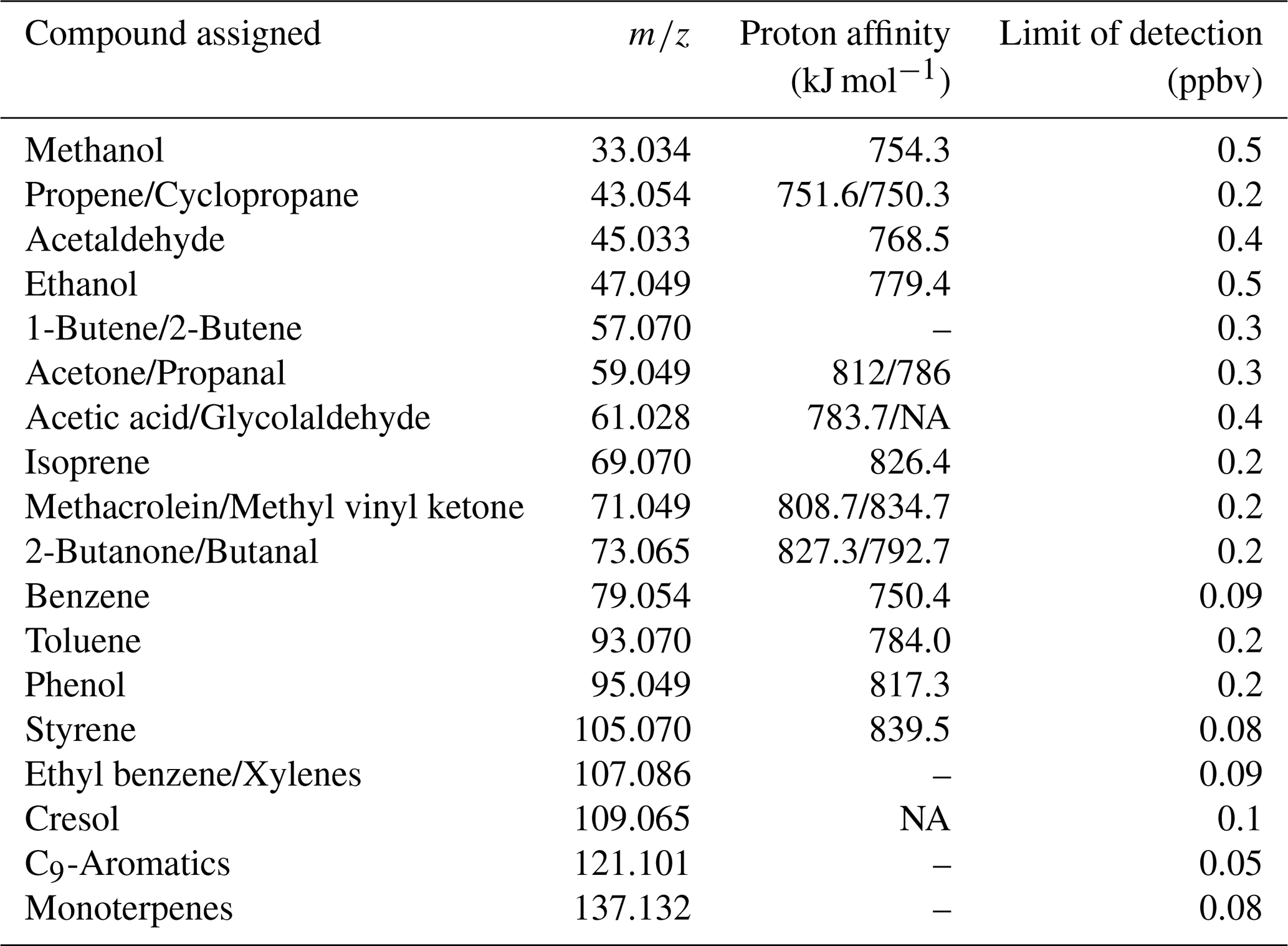
NA: not available

Appendix B: Time series of VOC measurements taken in Santiago

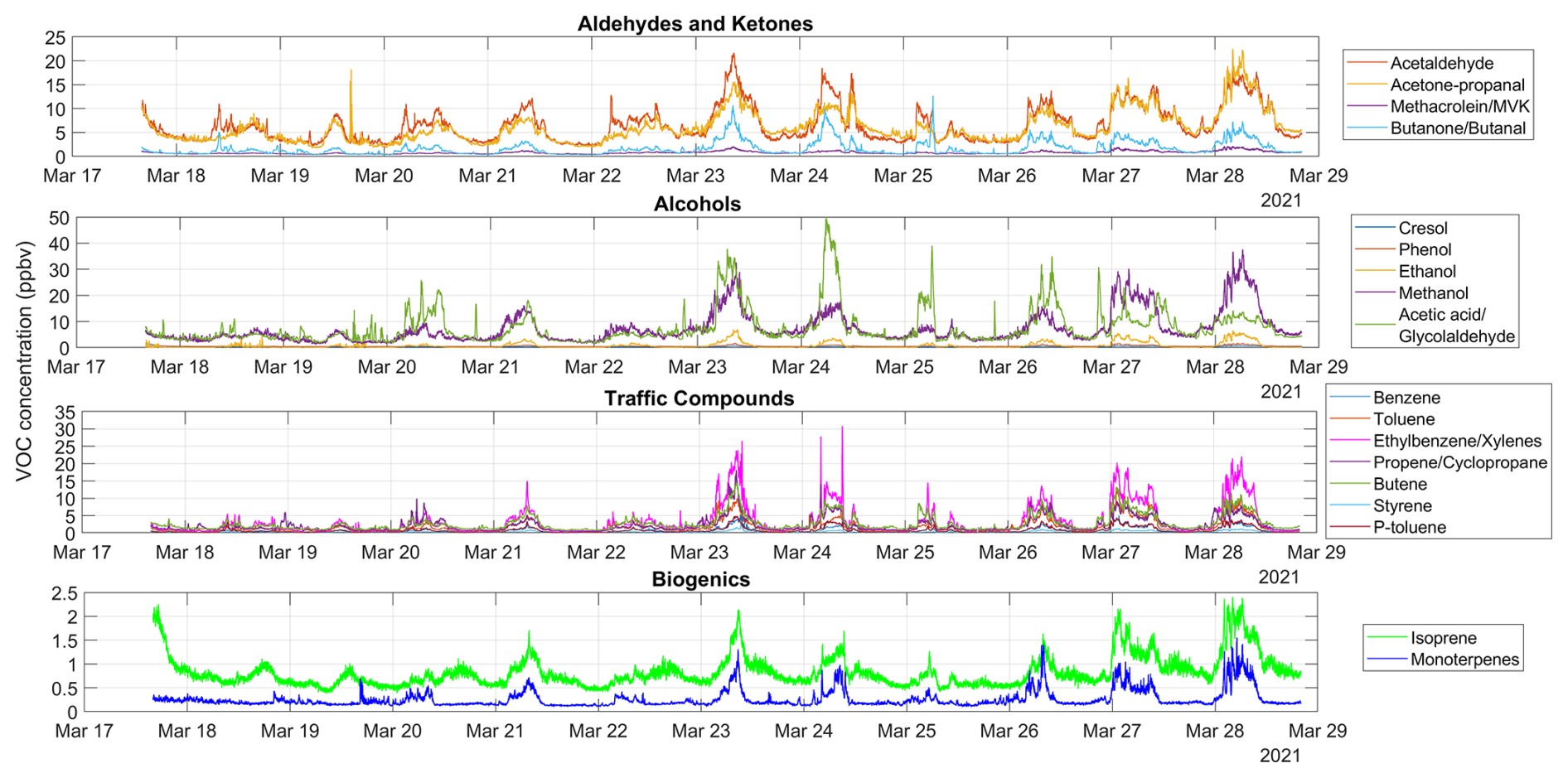
Figure B1 Time series (1 min data) of VOC measurements taken in Santiago, Chile from 17 to 28 March.