Kinematic properties of regions that can involve persistent contrails over the North Atlantic and Europe during April and May 2024

Contrails can last for many hours in the sky if they form in ice supersaturated regions (ISSRs). Contrail formation is possible once the ambient air is sufficiently moist and cold (below −40 °C). Contrails are persistent when the ambient relative humidity with respect to ice is at least 100 %. Cirrus clouds and contrails consist of ice crystals, which move with the wind. Ice supersaturation is an immaterial feature, which does not generally move with the wind. However, the movement of ISSRs relative to the winds is currently unknown. We analyse the movement of ISSRs and the wind using data for aviation weather forecasts, the WAWFOR package, from the German Weather Service (DWD). Our results demonstrate the kinematic differences and similarities of the movement of ISSRs in comparison to the wind. We show that the ISSRs on average move slower than the wind at the same location, the direction of movement is usually quite similar and the distributions of both velocities follow Weibull distributions. The almost identical direction of the movements is beneficial for contrail lifetimes, but the lifetime of contrails is not generally determined by the lifetime of ISSRs. Contrails are blown out of ISSRs with the wind. We assume that our study can be used as a basis for further analyses of the movement of ISSRs. Furthermore, our method of analysis is applicable to other extended features or areas, for instance to areas where aircraft non-CO₂ emissions would have a particularly large climate effect.

1 Introduction

Climate change is ongoing, and the necessity to take action against it is getting more and more pressing. All sectors have to reduce their share of the overall climate warming, including aviation. Although the latter sector currently contributes only about 3.5 % to the radiative forcing of climate, it cannot be exempted from urgent measures because aviation demand is increasing at a more rapid pace than the fuel need for a unit distance (the specific fuel consumption) is being reduced by commissioning of more efficient engines (Grewe et al., 2021; Lee et al., 2021). A peculiarity of aviation is its relatively strong climate impact induced by non-CO₂ emissions and effects. The individual non-CO₂ effects from a single flight depend strongly on the actual ambient conditions (synoptic weather situation, ambient cloudiness, position of the sun, etc.), which may open a possibility for climate friendly and environmentally friendly air transport by explicitly searching for routes where the climate impact is minimal (Matthes et al., 2021; Yin et al., 2023). An important part of climate-aware aviation is the avoidance of those persistent contrails that contribute to the warming of the climate. Persistent contrails can form if the so-called Schmidt–Appleman criterion, introduced by Schumann (1996), is fulfilled and when the flights transect a so-called ice supersaturated region (ISSR; see Gierens et al., 2012, for a review), where the relative humidity with respect to ice RH_i ≥ 100 %.

The Schmidt–Appleman criterion is often fulfilled once the ambient temperature is a few degrees below −40 °C. Supersaturation with respect to ice or in short ice supersaturation (ISS) occurs in particularly cold and humid regions in the troposphere, and it is primarily found in areas below the tropopause (Spichtinger et al., 2003; Petzold et al., 2020). Both conditions, low temperature and ice supersaturation, are found in regions that are termed cold ice supersaturated regions (CISSRs) by Irvine and Shine (2015). Ice supersaturated regions (ISSRs) arise mainly from large-scale vertical movements where rising air masses containing water vapour cool adiabatically and the relative humidity increases (Gierens and Brinkop, 2012). CISSRs and ISSRs are mostly the same areas since the Schmidt–Appleman criterion is most often fulfilled in ISSRs. ISS is often connected to slightly stable to neutral stratification because of the increases in the temperature gradient of rising air layers (Gierens et al., 2022).

ISSRs become visible either when natural cirrus clouds form or when aircraft fly through them because contrails that form in ISSRs are persistent and can remain in the sky for up to several hours. In spite of this close relation, contrails and their ambient ISSRs do not generally have the same lifetime (Bakan et al., 1994) and can also differ in their movement. Individual contrails and cirrus clouds may be driven out of the parental ISSR, which sooner or later terminates their existence when the ice crystals get into subsaturated air and sublimate. That is, contrails and cirrus on the one hand and ISSRs on the other have different lifetimes. The lifetime of ISSRs themselves is limited by the dynamics of the atmosphere. As soon as downdraft and thus adiabatic warming occurs, the ice supersaturation decreases and disappears eventually. The different lifetimes motivated us to study the differences between the real wind and the motion (pseudo-velocities) of ISSRs or, more precisely, CISSRs. A peculiar difference is that ISSRs have an initiation and an end in time, which also marks the end of their motion. In contrast, the wind is ceaseless (see the apt title of an old textbook, “The ceaseless wind” by Dutton, 1986).

For this initial study and the sake of simplicity, we consider horizontal motions only. We use data (see Reinert et al., 2024) from a weather forecast model that cover Europe and the North Atlantic and compare the motion of the air to the movement of CISSRs; that is, we compare the wind with a kind of pseudo-velocity. Unfortunately, only data from 2 months were available for this study, April and May 2024. But we have compared the wind distribution for this period with that from all other months in 12 different years to ascertain that the 2 selected months were not exceptional. The paper is organised as follows: first, we describe our data source in Sect. 2. Methods of the data analysis are compiled in Sect. 3. Results are presented in Sect. 4, and these are discussed in Sect. 5. At the end we conclude in Sect. 6.

2 Data

The German Weather Service (DWD) provides aviation weather forecasts four times per day (WAWFOR data), based on the weather forecast model ICON (Zängl et al., 2015), with hourly temporal resolution. The usual WAWFOR data inform aviation users on temperature, humidity, winds, etc. (WAWFOR Package 1), but for the German D-KULT project (Demonstrator Klima- und Umweltfreundlicher Lufttransport; Demonstration of climate-friendly and environmentally friendly air transport), additional datasets are produced that inform on the potential to form persistent contrails, i.e. on CISSRs, and on the climate effect of other gaseous emissions from aviation. The additional information that is used here is in particular as follows:

• PPC, the potential of persistent contrails – a binary value $(\mathrm{0}/\mathrm{1})$,

• PPC_prob, the probability of persistent contrails, the fraction of ensemble forecast members that have PPC = 1 – a real number between 0 and 1.

PPC is computed from the Schmidt–Appleman criterion (SAC) (Schumann, 1996) applying an overall propulsion efficiency of η = 0.365 and using temperature and relative humidity from the regular forecast. In order to compensate for a low humidity bias in the forecast (Gierens et al., 2022), situations with values of relative humidity with respect to ice (RH_i) in excess of 93 % are considered ice (super)-saturated (Hofer et al., 2024). PPC_prob is simply the number of members of the 40-member forecast ensemble that predict PPC = 1, divided by the total number of ensemble members (40). It can thus obtain values $n/\mathrm{40}$; n∈ℕ₀, 0 ≤ n ≤ 40. The meteorological data, PPC and PPC_prob, are available globally and with higher spatial resolution for the European region (EU nest, 0.0625° × 0.0625°, approx. 6.5 km × 6.5 km). The latter are used here in an area from 23.5° W to 62.5° E and 29.5 to 70.5° N. Altitudes that are most relevant for air traffic, between 8 and 12 km and with 0.5 km increments, are used. They correspond approximately to pressures $p\in (\mathrm{197},\mathrm{207},\mathrm{227},\mathrm{238},\mathrm{262},\mathrm{287},\mathrm{301},\mathrm{329},\mathrm{360})$ hPa.

PPC = 1 thus marks CISSR grid points where persistent contrails are possible, and PPC = 0 marks all the rest where either no contrails at all or merely short contrails can be formed. Only a few percent of ISSRs are not cold enough for contrail formation, but once a contrail is formed in a CISSR it can later spread into a slightly warmer ISSR (Wolf et al., 2023). Thus, we often simply write ISSR instead of CISSR. In addition, we use the wind data to compare them with the pseudo-velocity of ISSRs. The wind is given with its components in zonal (x) and meridional (y) directions.

The data cover April and May 2024. Due to missing data, 3 different days have been excluded: 30 April and 14 and 28 May. We use data for each day at the time of analysis 12 UTC+t hours, where $t\in (\mathrm{10},\mathrm{11},\mathrm{\dots },\mathrm{20})$ h.

We admit that an analysis of only 2 months does not allow us to draw general conclusions, but unfortunately, at the time of the study, more WAWFOR data of the additional sets were not available. It cannot be excluded that the 2 selected months have peculiarities in comparison to other seasons and other years. But a comparison of the wind directions and speeds over all 12 months and over 12 years, with months shuffled such that consecutive months are several years apart, did not point to any peculiarities (see Appendix D).

As we will see later, we always examine ISSRs that appear in three subsequent output times of a forecast run. The dataset contains 19 259 of these groups of ISSRs.

3 Methods

3.1 Identification of ISSR pairs

In order to determine the kinematics of ISSRs we consider PPC and PPC_prob in subsequent hourly outputs of the WAWFOR data. A pseudo-velocity of these regions is determined numerically in a way analogue to the numerical determination of a wind speed at a certain time. To determine the pseudo-velocity, V_ISSR(t_n), at a certain point in time, t_n (e.g. at time step n), the positions of the ISSR on the same pressure level at two additional times are needed, say at t_n−1 and t_n+1. It is thus necessary to identify ISSRs at these three points in time in the respective three outputs of the forecast. This task is solved first.

To identify ISSRs in several subsequent forecast steps (beginning with t_n and t_n−1), first their size (N, number of simply connected grid points, in longitude, latitude, and diagonally with PPC = 1) is determined. ISSRs consisting of fewer than 500 grid points are not considered further. We introduced the limit of 500 (N ≥ 500) to avoid examining small ISSR patches and to neglect this kind of noise. With 500 grid boxes, the length scale of ISSRs is about 145 km, quite close to that determined from in situ data (Gierens and Spichtinger, 2000; Spichtinger and Leschner, 2016). For all other ISSRs we calculate an analogue of a centre of mass, here termed centre of probability (COP) in the following way:

$$\begin{array}{}\text{(1)}& \begin{array}{l}{x}_{\mathrm{COP}}=\frac{{\sum }_{n=\mathrm{1}}^N{\text{PPC}}_{{\mathrm{prob}}_n}\cdot x_n}{{\sum }_{n=\mathrm{1}}^N{\text{PPC}}_{{\mathrm{prob}}_n}}\text{and}\\ y_{\mathrm{COP}}={\displaystyle \frac{{\sum }_{n=\mathrm{1}}^N{\text{PPC}}_{{\mathrm{prob}}_n}\cdot y_n}{{\sum }_{n=\mathrm{1}}^N{\text{PPC}}_{{\mathrm{prob}}_n}}}.\end{array}\end{array}$$

For the calculation, the spherical coordinates (longitude and latitude) are first converted into Cartesian coordinates (with the centre of the Earth as the origin), then the COP is determined in the Cartesian system, and finally the coordinates are transformed back into spherical coordinates to provide the longitude and latitude of each COP.

Thus, each ISSR has one centre of probability in each forecast and pressure level. Note that PPC = 1 for all points that belong to a distinct ISSR, while outside it is zero (PPC_prob can be non-zero, even if PPC = 0; the sums do not extend over such points). An example will follow later (see Sect. 3.6); the locations of the COPs are shown as red dots in Fig. 2. With the centres of probability at hand, Euclidean distances, d_i,j, of any pairs of COPs can be determined. ISSRs i, j are not identified if their distance exceeds 280 km.

However, for each ISSR at forecast time t_n we take the three closest ISSRs at forecast time t_n−1 into closer inspection for the identification with the respective ISSR at t_n, as long as these are less than 280 km apart. If there are no such candidates at t_n−1, the ISSR is not used for further analysis.

We assume 280 km as the maximum distance an ISSR can move within 1 h since the maximum wind speed in the data is 281 km h⁻¹.

A pair of ISSRs in a respective pair of forecasts must not change size N by more than 45 %. From the three candidates (the three closest ISSRs), if they fulfil this condition, the partner with the smallest d_i,j is selected. That is, a certain ISSR in 1 forecast hour is recognised in the adjacent forecast hour (previous or next). If the size condition is not met for the closest one, the second closest ISSR is chosen as a partner of the other time step. If this condition is not fulfilled for the two closest ISSRs, the third closest ISSR is chosen. If the condition is not fulfilled for this one either, no partner can be found in the other time step and this ISSR at time point t_n is not part of our analysis.

It may happen that more than one ISSR at time t_n has the same partner at time t_n−1. In this case we find a unique recognition via a measure of similarity provided by the Hu moments, in that we identify the pair having the smallest similarity difference (see Appendix A for more explanation). The other pair or pairs are not considered for the investigation. The same tests are performed between t_n+1 and t_n and only if an ISSR is recognised in all three forecasts, its kinematics can be determined. The last criterion refers to the fact that we do not consider ISSRs at the edges of our region, as they can distort the statistics. For this reason, the distance from each COP (at time t_n−1, t_n and t_n+1) to the upper, lower, right and left edge of our area (region: 23.5° W to 62.5° E and 29.5 to 70.5° N) is calculated. Only the ISSR triples are used where the COPs are at least 500 km away from the edge at all three times. For these ISSRs we calculate their kinematics, which is described in the next chapter.

3.2 Kinematics of ISSRs

To describe the dynamic motion of an ISSR, one needs to determine how fast it moves. This can be done in many ways, but the simplest way is chosen here; that is, the pseudo-velocity of an ISSR at t_n is taken as the Euclidean distance of its COP at t_n+1 and t_n−1 divided by the temporal difference:

$$\begin{array}{}\text{(2)}& {\displaystyle }{V}_{{\mathrm{ISSR}}_i}\left(t_n\right)={\displaystyle \frac{d\left(i,n+\mathrm{1},n-\mathrm{1}\right)}{t_{n+\mathrm{1}}-t_{n-\mathrm{1}}}},\text{where}\text{(3)}& {\displaystyle }\begin{array}{rl}& d\left(i,n+\mathrm{1},n-\mathrm{1}\right)\\ & =\sqrt{{\left[x_{{\mathrm{COP}}_i}\left(t_{n+\mathrm{1}}\right)-x_{{\mathrm{COP}}_i}\left(t_{n-\mathrm{1}}\right)\right]}^{\mathrm{2}}+{\left[y_{{\mathrm{COP}}_i}\left(t_{n+\mathrm{1}}\right)-y_{{\mathrm{COP}}_i}\left(t_{n-\mathrm{1}}\right)\right]}^{\mathrm{2}}}.\end{array}\end{array}$$

$V_{{\mathrm{ISSR}}_i}\left(t_n\right)$ is the pseudo-velocity of ISSR i at time t_n, $d(i,n+\mathrm{1},n-\mathrm{1})$ is the Euclidean distance of the COPs of ISSR i at the two time steps before and after t_n. In our case, the coordinates are given as longitude and latitude. The conversion of distances on a great circle to distances in kilometres is given in Appendix B.

In order to determine the direction of movement of an ISSR at t_n, the vector from its COP at t_n−1 to the COP at t_n+1 is used. Using the included angle between this vector and the zonal direction, the trigonometric functions and $V_{{\mathrm{ISSR}}_i}\left(t_n\right)$, the Cartesian components u_ISSR and v_ISSR of the ISSR can be determined.

3.3 Characterisation of the winds

As mentioned before, the velocity of the movement of the ISSRs and the wind speed are different. Since the wind and its Cartesian components u_wind and v_wind are only predicted for the grid points, the grid point that is closest to the centre of probability of an ISSR is selected. The magnitude of the wind speed is calculated using the components as follows:

$$\begin{array}{}\text{(4)}& V_{\mathrm{wind}}=\sqrt{u_{\mathrm{wind}}^{\mathrm{2}}+v_{\mathrm{wind}}^{\mathrm{2}}}.\end{array}$$

3.4 Angle between the motion of the ISSRs and the winds

The angle, δ, between the direction of motion of the ISSR and the direction of the local wind is the angle between the two vectors V_ISSR and V_wind with the following convention: if it needs an anti-clockwise rotation to turn from V_ISSR to V_wind, the angle δ > 0, otherwise δ ≤ 0. δ ranges from −180 to 180° (or −π ≤ δ ≤ π in radians). In order to retain the sign in this convention, we use the triple product, $\langle \cdot ,\cdot ,\cdot \rangle$, with the three unit vectors ${\widehat{\mathit{V}}}_{\mathrm{ISSR}}$, ${\widehat{\mathit{V}}}_{\mathrm{wind}}$, and $\widehat{\mathit{z}}$. The latter points upward into the vertical direction. A preliminary result is

$$\begin{array}{}\text{(5)}& {\mathit{\delta }}^{\prime }=\arcsin \left(\langle {\widehat{\mathit{V}}}_{\mathrm{ISSR}},{\widehat{\mathit{V}}}_{\mathrm{wind}},\widehat{\mathit{z}}\rangle \right).\end{array}$$

The result is not yet unique because the sin function is not unique in the range $[-\mathit{\pi },\mathit{\pi }]$. Thus, a second piece of information is obtained using

$$\begin{array}{}\text{(6)}& \cos {\mathit{\delta }}^{\prime \prime }={\widehat{\mathit{V}}}_{\mathrm{ISSR}}\cdot {\widehat{\mathit{V}}}_{\mathrm{wind}}.\end{array}$$

With this, the final result is

$$\begin{array}{}\text{(7)}& {\displaystyle }\begin{array}{rcl}\text{for}\cos {\mathit{\delta }}^{\prime \prime }>\mathrm{0}& :& \mathit{\delta }={\mathit{\delta }}^{\prime }\\ \text{for}\cos {\mathit{\delta }}^{\prime \prime }<\mathrm{0}\text{and}{\mathit{\delta }}^{\prime }<\mathrm{0}& :& \mathit{\delta }=-\mathit{\pi }-{\mathit{\delta }}^{\prime }\\ \text{for}\cos {\mathit{\delta }}^{\prime \prime }<\mathrm{0}\text{and}{\mathit{\delta }}^{\prime }>\mathrm{0}& :& \mathit{\delta }=\mathit{\pi }-{\mathit{\delta }}^{\prime }.\end{array}\end{array}$$

3.5 Rotation of ISSRs

As ISSRs are extended features, their characterisation with the COP is just the first of a series of conceivable moments. The second moments (inertia in the mechanical analogue) form a covariance matrix from which further characteristics can be derived via its eigenvalues and eigenvectors. The former can be used to compute an eccentricity of the ISSR, while the latter provide the principal axes of an ISSR.

For a given ISSR with N grid points the covariance matrix is

$$\begin{array}{}\text{(8)}& \begin{array}{rl}& \mathrm{\Theta }=\\ & \left(\begin{array}{ll}{\sum }_{n=\mathrm{1}}^N{\text{PPC}}_{{\mathrm{prob}}_n}\cdot (x_n-x_{\mathrm{COP}}{)}^{\mathrm{2}}& {\sum }_{n=\mathrm{1}}^N{\text{PPC}}_{{\mathrm{prob}}_n}\cdot (x_n-x_{\mathrm{COP}})\cdot (y_n-y_{\mathrm{COP}})\\ {\sum }_{n=\mathrm{1}}^N{\text{PPC}}_{{\mathrm{prob}}_n}\cdot (x_n-x_{\mathrm{COP}})\cdot (y_n-y_{\mathrm{COP}})& {\sum }_{n=\mathrm{1}}^N{\text{PPC}}_{{\mathrm{prob}}_n}\cdot (y_n-y_{\mathrm{COP}}{)}^{\mathrm{2}}\end{array}\right).\end{array}\end{array}$$

The calculation needs distances, not angles. Thus the necessary transformation is done before the application of Eq. (8). As Θ is a symmetric matrix, it has real eigenvalues and the eigenvectors are orthogonal. The eigenvector corresponding to the larger eigenvalue, V_PA, defines the principal axis (PA) and the other one the minor axis (MA) of the ISSR on the sphere. The direction of the axes may look strange because they are computed on the sphere; in the Euclidean geometry of a tangential plane the axes follow the projection of the ISSRs. However, the tangential plane moves as the COPs move, so they are not used to compute rotation rates. The example in Fig. 2 in Sect. 3.6 will show the principal axes in red (the extension in orange) and minor axes in yellow. The angle, α, between the principal axis at t_n−1 and t_n+1 is determined with the same convention as the angle δ from above: if it needs an anti-clockwise rotation to turn V_PA(t_n−1) onto V_PA(t_n+1), α > 0, otherwise α ≤ 0. The calculation of α is thus analogue to the calculation of δ:

$$\begin{array}{}\text{(9)}& \begin{array}{rl}& {\mathit{\alpha }}^{\prime }=\arcsin \left(\langle {\widehat{\mathit{V}}}_{\mathrm{PA}}\left(t_{n-\mathrm{1}}\right),{\widehat{\mathit{V}}}_{\mathrm{PA}}\left(t_{n+\mathrm{1}}\right),\widehat{\mathit{z}}\rangle \right),\\ & \cos {\mathit{\alpha }}^{\prime \prime }={\widehat{\mathit{V}}}_{\mathrm{PA}}\left(t_{n-\mathrm{1}}\right)\cdot {\widehat{\mathit{V}}}_{\mathrm{PA}}\left(t_{n+\mathrm{1}}\right),\end{array}\end{array}$$

and then the distinction of the cases (see Eq. 7) yields α.

α can be used to define a kind of angular velocity (pseudo-angular velocity) by dividing it by the temporal difference $t_{n+\mathrm{1}}-t_{n-\mathrm{1}}$:

$$\begin{array}{}\text{(10)}& \dot{\mathit{\alpha }}={\displaystyle \frac{\mathit{\alpha }}{t_{n+\mathrm{1}}-t_{n-\mathrm{1}}}}.\end{array}$$

Angular velocities are features of extended objects and thus not comparable to either the veering of the wind or its rotation, which are local quantities.

3.6 An example

An illustration of the methods and how they work is given in Figs. 1 and 2. The map of Fig. 1 shows the domain of the ICON-EU model. The coloured areas are CISSRs (PPC = 1) that are sufficiently large according to the conditions set out above. The different colours mark different individuals that should be identified in the same forecast run 1 h earlier and later. An identification in further forecast hours or even in forecasts with different initialisation times may be tried as well for the purpose of forecast verification. This has been done for the D-KULT project, but is not in the scope of the present paper.

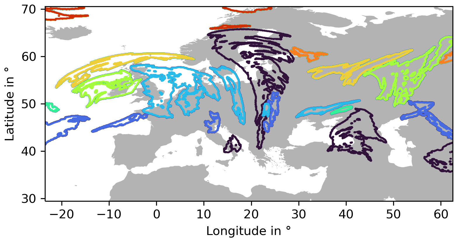
Figure 1 Map of the area covered by ICON-EU with regions where PPC = 1 (CISSRs) marked in different colours for the example situation from 4 April 2024 at 12:00 UTC initialisation for +15 h at approximately 301 hPa. These individual CISSRs may be identified in earlier and later forecast hours and in forecasts with differing initialisation time using the methods described in the text. Note that all ISSRs in the area under consideration are shown here. But ISSRs whose COPs are less than 500 km away from the edge are not included in the statistical analysis.

The characterisation of an individual CISSR is exemplified in Fig. 2. The coloured area again marks an individual CISSR. Its COP is located at the intersection of the coloured straight lines. Note that the COP lies not necessarily within the CISSR if the latter has a strongly bent shape. The red–orange lines are the major principal axes and the yellow ones the minor principal axes of the CISSRs.

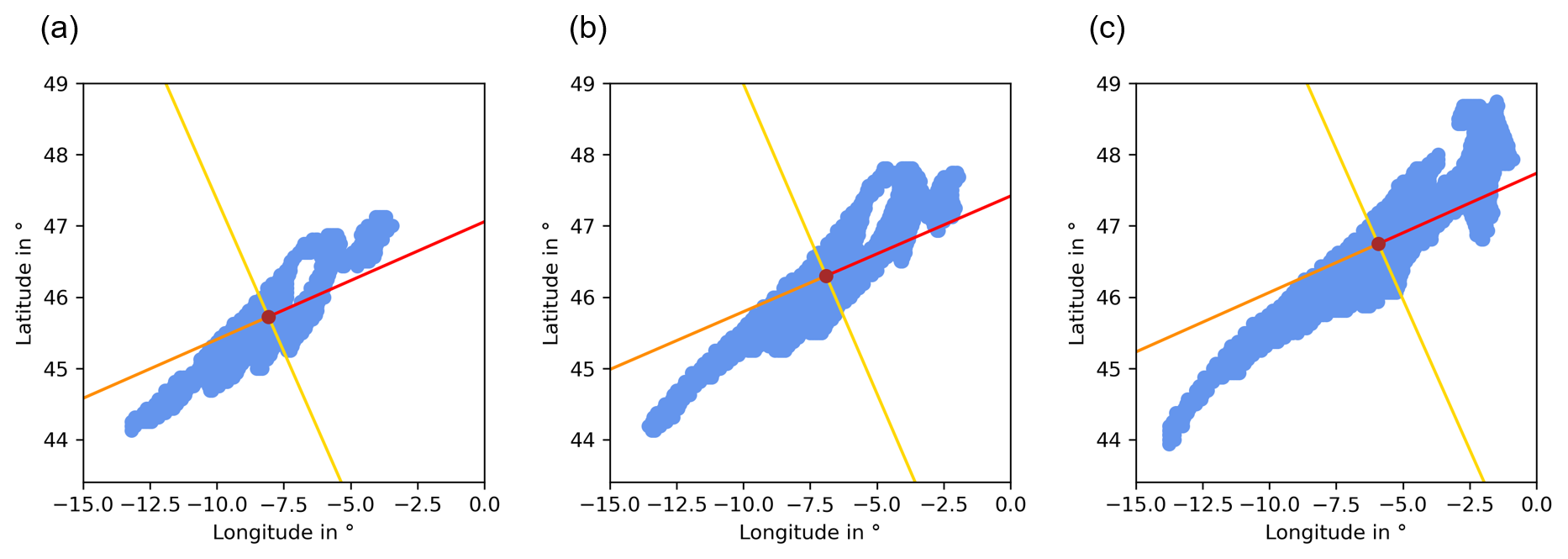
Figure 2 Basic characteristics of individual CISSRs: the CISSR, that is the grid points with PPC = 1 is marked in blue for t_n−1 (a), for t_n (b), and for t_n+1 (c). The centre of the crossed lines is the centre of probability (COP). The red–orange lines are the major principal axes and the yellow ones the minor principal axes of the CISSRs. Note that the CISSR in panel (b) corresponds to the dark-blue CISSR in Fig. 1 in the southwest between approximately −15 to 0° longitude and 43.4 to 49° latitude. The direction of the axes is computed on the sphere, and they therefore do not follow the flat projection that is shown in the figure.

4 Results

4.1 The relative motion of air and embedded ISSRs

4.1.1 Speeds

Figure 3a shows the histogram of pseudo-velocities of ISSRs calculated according to Eq. (2). The distribution of ISSR velocities has a mean and a standard deviation of 15.3 m s⁻¹ (black line) and 9.4 m s⁻¹ (blue lines), respectively. The median is 13.5 m s⁻¹ (red line). The distribution is right-skewed with a skewness of about 1.1. The corresponding distribution for the wind speeds at the COPs of the ISSRs, calculated according to Eq. (4), are shown in Fig. 3b. The distribution of wind velocities has a mean and a standard deviation of 20.6 m s⁻¹ (black line) and 10.6 m s⁻¹ (blue lines), respectively. The median is 19.4 m s⁻¹ (red line). The distribution is right-skewed with a skewness of about 0.6. Both distributions can be well approximated by a Weibull distribution (orange), a generalised exponential distribution, which is defined as follows:

$$\begin{array}{}\text{(11)}& f\left(v\right)=\mathit{\gamma }\cdot m\cdot v^{(m-\mathrm{1})}\cdot \exp \left(-\mathit{\gamma }\cdot v^m\right).\end{array}$$

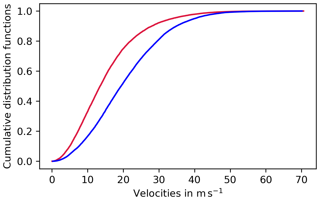
The two parameters m and γ can be determined by plotting the cumulative distribution functions (CDFs) of the pseudo-velocities of ISSRs V_ISSR and the wind speeds V_wind on a so-called Weibull paper (Gierens and Brinkop, 2002), where the x axis is log v and the y axis is $\log \left(\log (\mathrm{1}/(\mathrm{1}-\text{CDF}\left)\right)\right)$. For an illustration see Fig. C1 in Appendix C. In this representation, the two CDFs can be approximated by straight lines, which indicates that the original distributions can be approximated very well by Weibull distributions. The slopes are m_ISSR = 1.85 and m_wind = 1.95. The intercepts (s) are related to γ = e^s. These intercepts are s_ISSR = −5.2 and s_wind = −6.2, which are obtained by fitting the two lines to the CDFs in the Weibull paper. Compared to an exponential distribution (a Weibull distribution with m = 1) the two speed distributions with their m > 1 have quite different characteristics. At very low v the probability densities approach zero; that is very low wind and very slow motion of ISSRs hardly occurs in the study region. In contrast to an exponential, which maximises probability at zero, the considered speeds have mode values (maximum probability) at higher values, namely at 10.9 m s⁻¹ for ISSRs and 16.6 m s⁻¹ for the wind. Finally, Weibull distributions with m > 1 have lower tails than the exponential; this implies that high speeds would occur more often than observed if speeds were exponentially distributed.

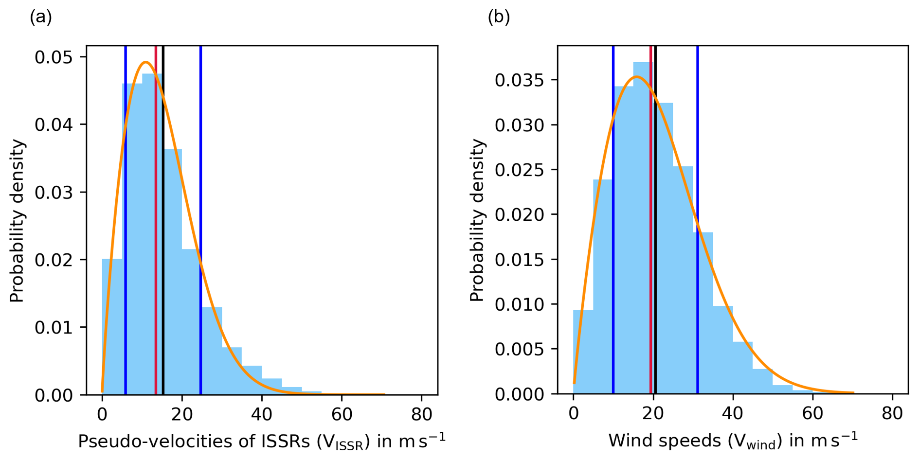
Figure 3 Histograms of pseudo-velocities of ISSRs (a) and wind speeds (b) in m s⁻¹. The histograms are normalised such that they present approximations of probability density functions, with a resolution of 5 m s⁻¹. Means (black lines) ± standard deviations (dark-blue lines) as well as the medians (red lines) are indicated. The orange curves show Weibull distributions that fit the histogram in panel (a) quite well and in panel (b) excellently. Please note the different scales on the y axes in both panels.

Wind data have been fitted by Weibull distributions already by Dixon and Swift (1984). Weibull distributions of wind speed are used by the wind energy business for the design of their installations and to estimate the expected gain (see, for example, Wais, 2017; Jung and Schindler, 2019). It seems that Weibull distributions are appropriate to model wind speed distributions both for the altitude of wind turbines and for the upper troposphere, although there is no theoretical justification for this (but read Weibull's remark on this problem, Weibull, 1951). As a test, we have evaluated wind speed statistics at 250 hPa in the study region for 12 months (every third day) in 12 different years (from ERA5 reanalyses, Hersbach et al., 2018), shuffled such that adjacent months are from years several years apart. For all months, the wind speed statistics closely follows a Weibull distribution (see Appendix D).

The distribution of individual differences of pseudo-velocities of ISSRs and of the wind speeds at ISSR COPs is nearly symmetric (the skewness is almost zero, 0.09) with a peak around 0 m s⁻¹; see Fig. 4. This means that the velocities of ISSRs and the wind in the COP hardly differ in most cases. The mean of the distribution is −5.3 m s⁻¹ (black), and the standard deviation is 11.8 m s⁻¹ (blue). The median of this distribution is −5.0 m s⁻¹ (red). To characterise the peaked shape of the distribution, we use the excess kurtosis, which is the standardised central fourth moment of a distribution minus 3 (the normal distribution has a kurtosis of 3). Positive excess kurtosis values indicate a more pointed and steeper distribution, while negative values indicate a flatter distribution than the normal.

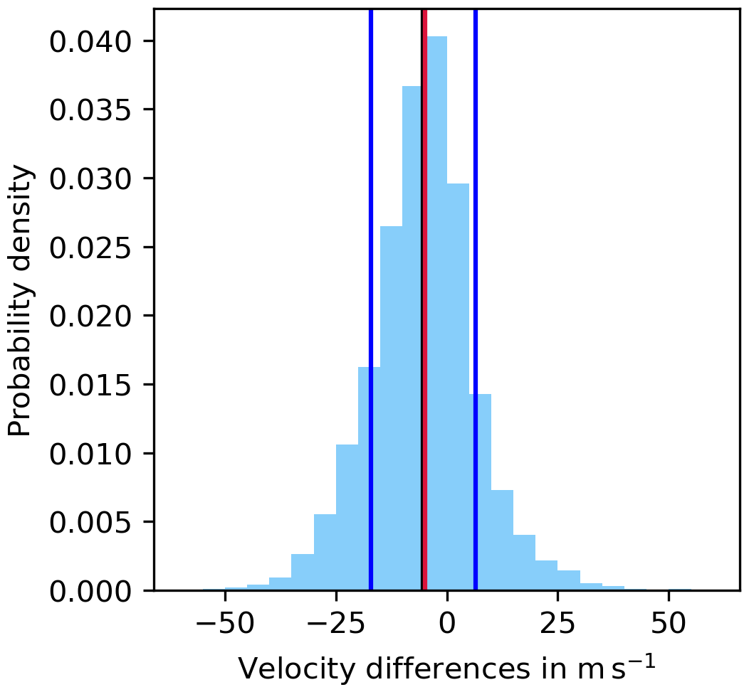
Figure 4 Histogram of velocity differences: pseudo-velocities of ISSRs minus the wind speeds in m s⁻¹. The histogram is normalised, such that it represents an approximation of the corresponding probability density, with a resolution of 5 m s⁻¹. The mean (black line) ±1 standard deviation (dark-blue lines) are indicated as well as the median (red line).

As expected for a peaked distribution, the kurtosis (1.2) exceeds zero significantly, if we estimate its uncertainty with $\mathit{\delta }\left(\text{kurtosis}\right)\approx \sqrt{(\mathrm{24}/N)}$ ≈ 0.035, where N = 19 259 is the number of data in the histogram (Press et al., 1989 p. 457). In rare cases the speed differences exceed 50 m s⁻¹ in both directions.

Figure 5 shows a joint histogram for ISSR pseudo-velocities and wind speeds. The highest density of cases is at low pseudo-velocities of ISSRs with slightly higher wind speeds. In order to see whether the two (marginal) distributions of the pseudo-velocities of ISSRs and of the wind speeds differ significantly, we perform a Kolmogorov–Smirnov test on the pair of their corresponding cumulative distribution functions ($F_{V_{\mathrm{ISSR}}}$ and $F_{V_{\mathrm{wind}}}$); see Fig. 6. To do this, we test the null hypothesis H₀ that $F_{V_{\mathrm{ISSR}}}$ = $F_{V_{\mathrm{wind}}}$, which states that the two distributions are equal. The alternative hypothesis H₁ is $F_{V_{\mathrm{ISSR}}}$ ≠ $F_{V_{\mathrm{wind}}}$, i.e. that the two distribution functions do not match. We select a significance level α = 5 %. If H₀ is rejected on this level, H₁ can be accepted, and the likelihood that this result is wrongly obtained by chance is less than 5 %. For the test, the maximum vertical distance D between the two CDFs ($F_{V_{\mathrm{ISSR}}}$ and $F_{V_{\mathrm{wind}}}$) is determined. The larger this distance, the more likely H₀ is rejected. The test statistic D and the p value are calculated using the statistics software package R, which yields D ≈ 0.24 and a p value so much smaller than the significance level that the exact choice of α does not matter: the null hypothesis H₀ can firmly be rejected and the two distributions, $F_{V_{\mathrm{ISSR}}}$ and $F_{V_{\mathrm{wind}}}$, differ significantly from each other.

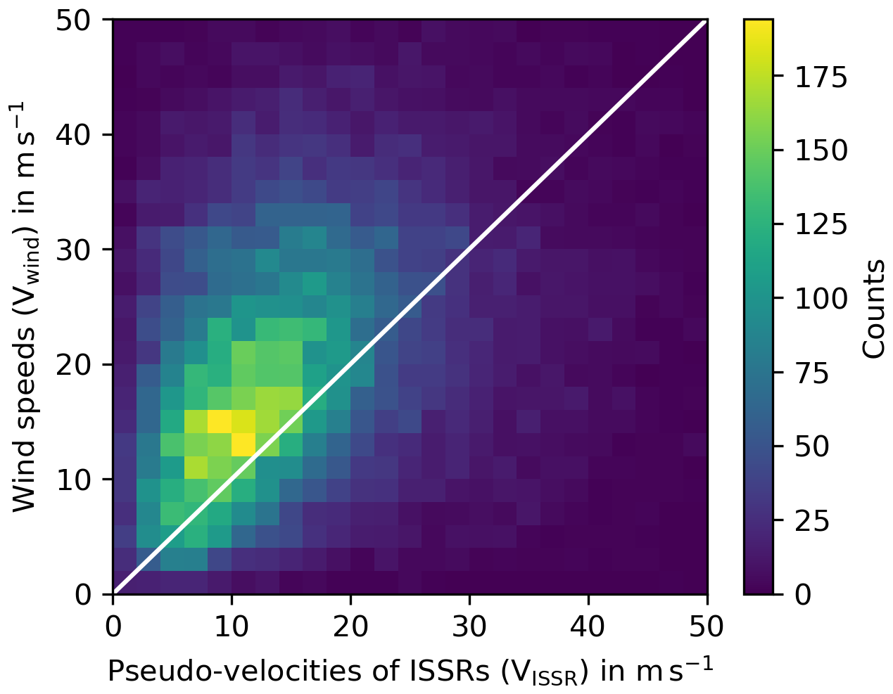
Figure 5 Joint histogram of ISSR pseudo-velocities and real air wind speeds at the position of the ISSR COPs. The number of joint occurrences in 2 m s⁻¹ × 2 m s⁻¹ square bins is given in the colour bar. The white diagonal marks the points where the two speeds are equal (or nearly so). Higher speeds than 50 m s⁻¹ occur in our data, but very rarely.

Figure 6 Cumulative distribution functions $F_{V_{\mathrm{ISSR}}}$ (red) and $F_{V_{\mathrm{wind}}}$ (blue).

Finally, we study the (linear) correlation between the ISSR speeds and the wind speeds. It measures how the individual ISSR speeds deviate from their mean in a positive or negative direction when simultaneously the wind speeds deviate positively or negatively from their mean and vice versa. It is important to note that the correlation compares anomalies, not the absolute values. This quantity is given as

$$\begin{array}{}\text{(12)}& \begin{array}{rl}& \text{Corr}\left(V_{\mathrm{ISSR}},V_{\mathrm{wind}}\right)\\ & ={\displaystyle \frac{\mathrm{1}}{{\mathit{\sigma }}_{V_{\mathrm{ISSR}}}{\mathit{\sigma }}_{V_{\mathrm{wind}}}}}\sum _i\left(V_{\mathrm{ISSR},i}-\langle V_{\mathrm{ISSR}}\rangle \right)\left(V_{\mathrm{wind},i}-\langle V_{\mathrm{wind}}\rangle \right),\end{array}\end{array}$$

where the σ_x are the two standard deviations, and the means are indicated with angular brackets. The sum extends over all our cases. We find quite a moderate correlation of 0.32 for the two speed anomalies. This might seem surprising since the absolute speed differences are mainly small. But it simply indicates that the speed differences are positive and negative with similar probability.

In some cases, there are significant velocity differences between the motion of ISSRs and the wind (as can be seen in Fig. 4 due to the large standard deviation). For the case of the largest speed difference (61.27 m s⁻¹), the synoptic situation was examined more closely (4 April 2024, at 00:00 UTC). It turned out that for this specific case the two COPs 1 h before and after t_n are almost on top of each other, while the COP at t_n lies further west of it. Thus, the vector from t_n−1 to t_n+1 is also very short, which means that the resulting velocity for the ISSR movement at t_n is very low. The wind, however, blows strongly to the east. In addition, east of the COPs, strong upward movements can be observed, where new air is constantly being supplied from below, which cools and increases its RH_i. This means that new ISS is constantly being created (or enlarged) at this point, while the horizontal wind simply moves on. The gradient of the vertical wind would probably show a maximum at this location. However, this case study only shows the explanation for the case of the maximum speed difference. There are also other cases with significant differences, but not all of them can be examined within the scope of this work. However, this would be very interesting for further analysis.

4.1.2 Directions

Next, we consider the direction of the movement of the ISSRs and the wind at their COPs separately, where 0° refers to movement to the north, and 90° corresponds to eastward motion; see Fig. 7. (Please note that this convention is different from meteorological use; it is rather oriented on a compass. We use eastward wind instead of west wind, for instance.) Both histograms show that the most frequent direction of motion of ISSRs and of the winds at ISSR COPs is eastward. There is also a second maximum in the westward direction for the direction of ISSR movements, but this is much weaker than the eastward maximum. The similarity of the histograms does not necessarily imply that the motion of an ISSR and the wind at its COP are often aligned as the histograms show the statistics of both quantities separately. To check this, we consider again a two-dimensional histogram, that is, the joint probability of the directions of motion (see Fig. 8). This shows that both ISSRs and the wind usually move in very similar directions; that is, the motions are aligned.

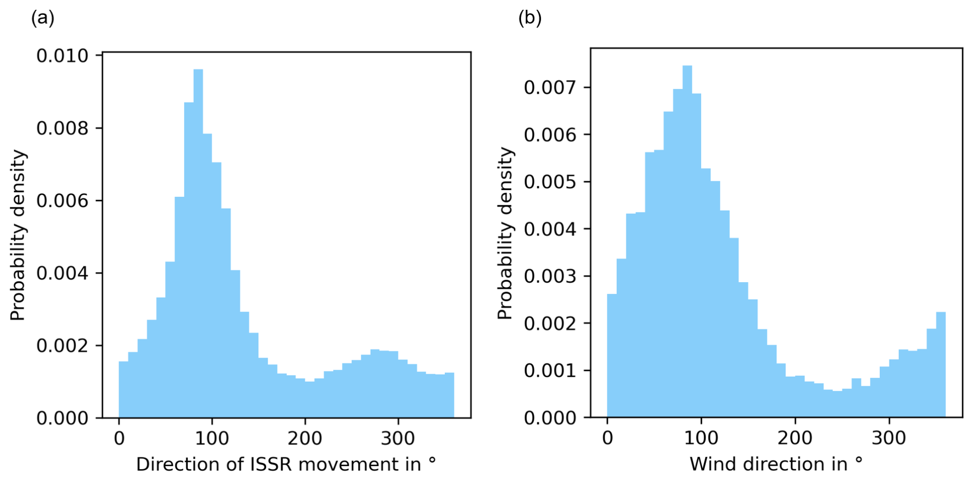
Figure 7 Histograms of the direction of movement of ISSRs (a) and the wind at their COPs (b). Angles range from 0 to 360°, where 0 or 360° means movement to the north, 90° a movement to the east, and so on. The histograms are normalised, such that they represent approximations of the corresponding probability densities, with a resolution of 10°. The histograms are very similar. Both have their maximum between 80 and 90°, which indicates a predominant west-to-east movement.

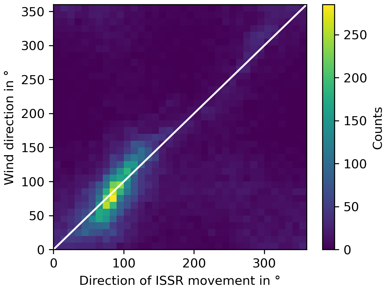
Figure 8 Joint probability distribution of the direction of motion of ISSRs and the wind at their COPs. The number of joint occurrences in 10° × 10° square bins is given in the colour bar. The white diagonal marks the points where the two directions are equal (or nearly so). The alignment is quite strong.

Figure 9 shows the differences of both directions of motion. In this histogram, a positive angle means the angle from the ISSR vector in an anti-clockwise direction to the wind vector. The mean angle is 3.5° with a standard deviation of 63.7°. The median is 1.9°. If their directions differ then the difference is slightly more common in the anti-clockwise direction than in the clockwise direction. The peaked shape of the distribution at 0° again shows the quite strong directional alignment of ISSRs and winds. However, the standard deviation is not small, and thus cases with quite different directions of motion are no exceptions. The differences in directions and speed mean that air parcels belonging to an ISSR will leave it sooner or later. Consequences for contrail lifetimes are analysed using trajectory calculations by Hofer and Gierens (2025b).

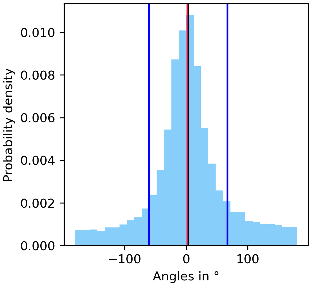
Figure 9 Histogram of the angles (in degree) between the movement of ISSRs (vector of COP at t_n−1 and COP at t_n+1) and wind vectors from −180 to 180°. Positive angles mean anti-clockwise rotation from the ISSR vector to the wind vector. The histogram is normalised, such that it represents an approximation to a probability density function, with a resolution of 12°. Mean ±1 standard deviation are indicated with the black and blue lines and the median with a red line, respectively.

4.2 Rotation of ISSRs

The rotation of ISSRs is treated as the rotation of its principal axes in time. This can be caused by a real rotation (if the whole system rotates), but a change of the shape or the spatial distribution of probability around the COP can induce rotation of the principal axes as well; thus it is appropriate to speak of a pseudo-rotation with a corresponding pseudo-angular speed. Figure 10 shows a histogram of the pseudo-angular speed of ISSRs. It is remarkably symmetric around zero (the skewness is almost zero) and peaks at zero. That is, ISSRs most often do hardly rotate, and if so, they do it with similar probability in clockwise and anti-clockwise directions. Accordingly, both mean and median are very nearly 0° h⁻¹ (black and red line) with a standard deviation of 20.5° h⁻¹ (blue lines).

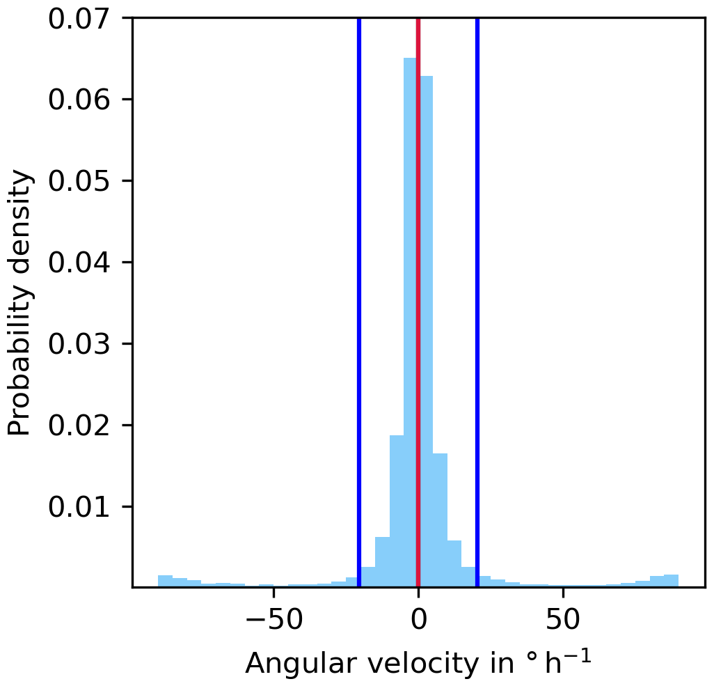
Figure 10 Histogram of the differences in angles between the principal axis of t_n−1 and principal axis of t_n+1 covered within 2 h, i.e. the angular velocity $\dot{\mathit{\alpha }}$ (in ° h⁻¹). The histogram is normalised, such that it represents an approximation of the corresponding probability density, with a resolution of 5° h⁻¹. The mean (black line) ±1 standard deviation (dark-blue lines) are indicated as well as the median (red line). Note that the median and the mean are nearly the same. For this reason the latter one can hardly be seen.

5 Discussion

5.1 Discussion of the methods

This analysis was constrained to horizontal movement only, for the sake of simplicity. This means that the vertical movement of ISSRs was not taken into account. This might seem surprising since vertical lift of moist air is the primary source of ice supersaturation (Gierens et al., 2012). However, vertical movements are 2 to 3 orders of magnitudes smaller than horizontal movements in the atmosphere. Therefore we think that this simplification may be justified. Anyway, vertical movements of ISSRs could pretend horizontal movements (e.g. by shape changes) or could perturb the identification of ISSRs in consecutive forecasts if, for example, uplifting air leads to new supersaturation popping up on the considered pressure level close to an ISSR that already exists on that level.

Two ISSRs can also coagulate to a single one or vice versa. In principle, the mechanistic parts of this study (i.e. determination of the COP and the principal axes) can be performed in three dimensions straightforwardly, but the problems with the identification of ISSRs in consecutive forecasts would become much more involved. For instance, the application of the Hu moments would not be possible. Therefore, this study constrains the analysis to two dimensions.

ISSRs are not rigid bodies; they generally change shape, extension and total probability while they move and rotate. Thus, one could think of dividing their kinematic properties into internal and external effects, internal being the change in shape and total probability and external being the “true” shift and rotation. Both internal and external effects change the COP and the principal axes, but it is very difficult and perhaps even impossible or useless to disentangle internal and external effects. One could argue that external effects are caused by shifts and rotation of the carrier fluid air that contains the ISSR; that is, it would be characterised by V_wind and a large-scale rotation of the air. Then the difference V_ISSR−V_wind would be completely due to internal changes in the shape, extension, and probability distribution of an ISSR.

Considering rotation, the situation is analogous, but also numerically quite difficult. A large-scale rotation of the air could be given by the circulation of the wind along the perimeter of an ISSR which, however, is not well defined in a discrete model space. Similarly, the partition of rotation of the ISSR into external and internal cannot be computed adequately since rotation is not well defined in discrete spaces (e.g. Thibault, 2010). Because of these unsolved problems, we have not tried to separate V_ISSR or $\dot{\mathit{\alpha }}$ into external and internal contributions.

We admit that the study is based on only 2 months of data, and it is confined to the EU-nest of the ICON model. As the atmospheric dynamics which is at the base of our findings changes seasonally and geographically, the relation between ISSR motion and the motion of the ambient wind may change from season to season and geographically, in particular in the meridional direction. As a basic test for seasonal and/or interannual variations we have checked that wind speed statistics follow Weibull distributions with nearly equal exponent over all the selected months (January to December) and years (2013–2024), at least for the considered study region. From this it seems that April and May 2024 have a quite usual wind speed distribution.

5.2 Implications for contrail lifetimes

It turned out that ISSRs move very often with similar speeds and in similar directions to the wind as their COPs do. A similar direction of the movements implies that contrails are not easily blown out of their ambient ISSRs, which favours the growth of their ice crystals. In such cases contrails end once their crystals are sufficiently large for sedimentation or once the ice supersaturation itself vanishes by subsidence, increasing temperature and thus decreasing relative humidity. However, contrail lifetimes are not controlled by the lifetime of their parent ISSR for the rare cases where wind and ISSR directions differ. In such cases contrails are blown out of the ISSR with the wind. The reverse process is not possible; persistent contrails cannot be blown into an ISSR because if a contrail does not form within an ISSR, it evaporates quickly so there is nothing left to be blown into the ISSR. Thus, individual contrails must have a shorter lifetime on average than their parental ISSR exists. This is shown by Hofer and Gierens (2025b), who performed trajectory calculations for air parcels that initially reside within an ISSR. The individual air parcels are followed until they eventually either leave the ISSR or until the relative humidity itself falls under ice saturation. This leads to a statistics of “survival” times (again a Weibull distribution), which allows us to derive a synoptic timescale for contrail termination. This timescale is a few hours, which is consistent with results from satellite tracking of contrails (Gierens and Vázquez-Navarro, 2018).

However, an ISSR may be always filled with new contrails if new aircraft cross it, producing new contrails. This was observed 30 years ago by Bakan et al. (1994).

5.3 Application to other features

The presented method was originally developed for the verification of forecasts of CISSRs. An older forecast is to be compared to a newer forecast for the same valid time. The latter forecast serves as a proxy for the reality that is not otherwise available. With the mechanical method we simply determine the COPs and principal axes of individual CISSRs in both forecasts, additionally to their size and total probability, and calculate the individual differences (or other statistics if desired). We note that the method can be used for other features as well, for instance in areas where aircraft non-CO₂ emissions would have a particularly large climate effect. For this purpose, we would use the (algorithmic) climate change function fields (Dietmüller et al., 2023; Yin et al., 2023), select a threshold (which isolates maxima), and use the value of the aCCF (or the excess over the threshold) in place of the PPC_prob. Then everything else is completely analogous to the analyses presented in the current paper.

6 Conclusions

In this study, DWD WAWFOR data from 2 months are analysed to obtain information about the movement of ice supersaturated regions (ISSRs) and to compare this with the local wind at the ISSRs. To this end we use humidity, temperature, and wind information and determine the location of ISSRs. We develop a procedure to identify ISSRs in three consecutive forecasts. For each ISSR we determine a centre of probability (COP) and the principal axes at this point. Speeds of ISSRs are determined by the movement of the COPs together with rotations of their principal axes. For these positions the wind speeds and the rotation of the wind vectors are recorded. These data form the basis of our comparisons. On average, the wind speeds are larger than the ISSR movement speed. The mean of the pseudo-velocities of ISSRs is approximately 15 m s⁻¹. The mean of the wind speeds is around 21 m s⁻¹. Both distributions, the ISSR speed and the wind speed, follow a Weibull distribution very well. In most cases ISSRs move at a similar speed as the local wind. An analogous statement pertains to the directions of the movement. Both ISSRs and the local wind move in most cases in an eastward direction. Extended ISSRs not only move straight forward but also rotate, but quite slowly. Within 1 h the rotation angle rarely exceeds ±10°. Clockwise and anti-clockwise rotations occur with almost equal probability.

The study results imply that persistent contrails, which move with the wind, should often move parallel to and inside their parent ISSR. Under this condition, the lifetime of contrails is constrained by the sedimentation of ice crystals or by the end of the lifetime of the ISSR itself. Once ISSRs and the wind move in different directions, contrails are blown out of the ISSR into the subsaturated environment and vanish.

Finally, we note that the methods used in this paper can be applied to other extended features in the atmosphere in an analogous way. One can determine the centre of mass and the principal axes for any 2-dimensional coherent and closed feature in a weather map with the current methods, at least after suitable adaptations (for instance replacement of PPC and PPC_prob). If the same feature can be delineated on, say satellite data, or if the same features are compared in various forecasts (with different time horizons of from different forecast models), there is the possibility of comparison and checking the plausibility of the features under consideration quantitatively using the centres of mass and the principal axes. As an example, one could use the algorithmic climate change functions (Dietmüller et al., 2023; Yin et al., 2023) from the WAWFOR-Klima data, set a threshold value, and define everything where the threshold is exceeded as a feature. Our method can then be applied. Then one might use the 40 ensemble members of ICON to see how these features behave over the whole ensemble to check whether the considered forecast produces a coherent or incoherent picture of the situation.

Appendix A: Hu moments

Hu moments are based on normalised central moments. The general formula of normalised central moments in our application is

$$\begin{array}{}\text{(A1)}& {\mathit{\eta }}_{k,l}={\displaystyle \frac{{\sum }_x{\sum }_y{\text{PPC}}_{\mathrm{prob}}(x,y)\cdot {\left(x-x_{\mathrm{COP}}\right)}^k\cdot {\left(y-y_{\mathrm{COP}}\right)}^l}{{\left[{\sum }_x{\sum }_y{\text{PPC}}_{\mathrm{prob}}(x,y)\right]}^{\mathrm{1}+\frac{k+l}{\mathrm{2}}}}}.\end{array}$$

All η_k,l values, for which k+l = 2, are related to the entries of the covariance matrix Θ (see Eq. 8).

Normalised central moments are invariant to translation and scale. The advantage of the seven Hu moments is that they are invariant to translation, scale and rotation. The first six Hu moments are also invariant to reflection; however, for the seventh Hu moment the sign changes for reflection. The Hu moments can be calculated this way (Prokop and Reeves, 1992; Huang and Leng, 2010; Mallick and Bapat, 2018):

$$\begin{array}{}\text{(A2)}& {\displaystyle }{h}_{\mathrm{1}}={\mathit{\eta }}_{\mathrm{20}}+{\mathit{\eta }}_{\mathrm{02}}\text{(A3)}& {\displaystyle }{h}_{\mathrm{2}}={\left({\mathit{\eta }}_{\mathrm{20}}-{\mathit{\eta }}_{\mathrm{02}}\right)}^{\mathrm{2}}+\mathrm{4}\cdot {\mathit{\eta }}_{\mathrm{11}}^{\mathrm{2}}\text{(A4)}& {\displaystyle }{h}_{\mathrm{3}}={\left({\mathit{\eta }}_{\mathrm{30}}-\mathrm{3}\cdot {\mathit{\eta }}_{\mathrm{12}}\right)}^{\mathrm{2}}+\left(\mathrm{3}\cdot {\mathit{\eta }}_{\mathrm{21}}-{\mathit{\eta }}_{\mathrm{03}}^{\mathrm{2}}\right)\text{(A5)}& {\displaystyle }{h}_{\mathrm{4}}={\left({\mathit{\eta }}_{\mathrm{30}}+{\mathit{\eta }}_{\mathrm{12}}\right)}^{\mathrm{2}}+{\left({\mathit{\eta }}_{\mathrm{21}}+{\mathit{\eta }}_{\mathrm{03}}\right)}^{\mathrm{2}}\text{(A6)}& {\displaystyle }\begin{array}{rl}{h}_{\mathrm{5}}=& \left({\mathit{\eta }}_{\mathrm{30}}-\mathrm{3}\cdot {\mathit{\eta }}_{\mathrm{12}}\right)\cdot \left({\mathit{\eta }}_{\mathrm{30}}+{\mathit{\eta }}_{\mathrm{12}}\right)\\ & \cdot \left[{\left({\mathit{\eta }}_{\mathrm{30}}+{\mathit{\eta }}_{\mathrm{12}}\right)}^{\mathrm{2}}-\mathrm{3}\cdot {\left({\mathit{\eta }}_{\mathrm{21}}+{\mathit{\eta }}_{\mathrm{03}}\right)}^{\mathrm{2}}\right]\\ & +\left(\mathrm{3}\cdot {\mathit{\eta }}_{\mathrm{21}}-{\mathit{\eta }}_{\mathrm{03}}\right)\cdot \left({\mathit{\eta }}_{\mathrm{21}}+{\mathit{\eta }}_{\mathrm{03}}\right)\\ & \cdot \left[\mathrm{3}\cdot {\left({\mathit{\eta }}_{\mathrm{30}}+{\mathit{\eta }}_{\mathrm{12}}\right)}^{\mathrm{2}}-{\left({\mathit{\eta }}_{\mathrm{21}}+{\mathit{\eta }}_{\mathrm{03}}\right)}^{\mathrm{2}}\right]\end{array}\text{(A7)}& {\displaystyle }\begin{array}{rl}{h}_{\mathrm{6}}=& \left({\mathit{\eta }}_{\mathrm{20}}-{\mathit{\eta }}_{\mathrm{02}}\right)\cdot [{\left({\mathit{\eta }}_{\mathrm{30}}+{\mathit{\eta }}_{\mathrm{12}}\right)}^{\mathrm{2}}-{\left({\mathit{\eta }}_{\mathrm{21}}+{\mathit{\eta }}_{\mathrm{03}}\right)}^{\mathrm{2}}\\ & +\mathrm{4}\cdot {\mathit{\eta }}_{\mathrm{11}}\cdot \left({\mathit{\eta }}_{\mathrm{30}}+{\mathit{\eta }}_{\mathrm{12}}\right)\cdot \left({\mathit{\eta }}_{\mathrm{21}}+{\mathit{\eta }}_{\mathrm{03}}\right)]\end{array}\text{(A8)}& {\displaystyle }\begin{array}{rl}{h}_{\mathrm{7}}=& \left(\mathrm{3}\cdot {\mathit{\eta }}_{\mathrm{21}}-{\mathit{\eta }}_{\mathrm{03}}\right)\cdot \left({\mathit{\eta }}_{\mathrm{30}}+{\mathit{\eta }}_{\mathrm{12}}\right)\\ & \cdot \left[{\left({\mathit{\eta }}_{\mathrm{30}}+{\mathit{\eta }}_{\mathrm{12}}\right)}^{\mathrm{2}}-\mathrm{3}\cdot {\left({\mathit{\eta }}_{\mathrm{21}}+{\mathit{\eta }}_{\mathrm{03}}\right)}^{\mathrm{2}}\right]\\ & +\left({\mathit{\eta }}_{\mathrm{30}}-\mathrm{3}\cdot {\mathit{\eta }}_{\mathrm{12}}\right)\cdot \left({\mathit{\eta }}_{\mathrm{21}}+{\mathit{\eta }}_{\mathrm{03}}\right)\\ & \cdot \left[\mathrm{3}\cdot {\left({\mathit{\eta }}_{\mathrm{30}}+{\mathit{\eta }}_{\mathrm{12}}\right)}^{\mathrm{2}}-{\left({\mathit{\eta }}_{\mathrm{21}}+{\mathit{\eta }}_{\mathrm{03}}\right)}^{\mathrm{2}}\right].\end{array}\end{array}$$

Since the seven Hu moments have different orders of magnitude and are therefore difficult to compare, they are adjusted using a log transformation:

$$\begin{array}{}\text{(A9)}& H_i=-\text{sgn}\left(h_i\right)\cdot \log \left(\right|h_i\left|\right).\end{array}$$

These log-transformed H_i values are then combined, and a difference can be calculated that reflects the similarity difference between two forms of ISSR A and ISSR B:

$$\begin{array}{}\text{(A10)}& D(A,B)=\sum _{i=\mathrm{1}}^{\mathrm{7}}|{\displaystyle \frac{\mathrm{1}}{H_i^B}}-{\displaystyle \frac{\mathrm{1}}{H_i^A}}|.\end{array}$$

In order to identify two shapes of ISSR A and ISSR B in subsequent forecasts, D(A,B) should be as small as possible.

Appendix B: Distances on great circles

The distance between two points with longitudes λ_1,2 and latitudes φ_1,2 on a sphere can be determined using the equations for an orthodrome, i.e. the shortest connection between two points on a sphere (see any textbook on navigation or spherical geometry and trigonometry). Let us assume that λ_1,2 and φ_1,2 are given in radians. Let Δ_λ = |λ₁ − λ₂|. Then the distance, d_1,2, on the surface of the Earth is given as

$$\begin{array}{}\text{(B1)}& \begin{array}{rl}{d}_{\mathrm{1},\mathrm{2}}& =R\arccos \\ & \left[\sin \left({\mathit{\phi }}_{\mathrm{1}}\right)\sin \left({\mathit{\phi }}_{\mathrm{2}}\right)+\cos \left({\mathit{\phi }}_{\mathrm{1}}\right)\cos \left({\mathit{\phi }}_{\mathrm{2}}\right)\cdot \cos \left({\mathrm{\Delta }}_{\mathit{\lambda }}\right)\right],\end{array}\end{array}$$

with the radius of the Earth R ≈ 6373 km. If the longitudes and latitudes are given in degrees, they must be translated into radians with the factor $\mathit{\pi }/\mathrm{180}$°.

Appendix C: Cumulative distribution functions of the pseudo-velocities of ISSRs and the wind speeds plotted on Weibull paper

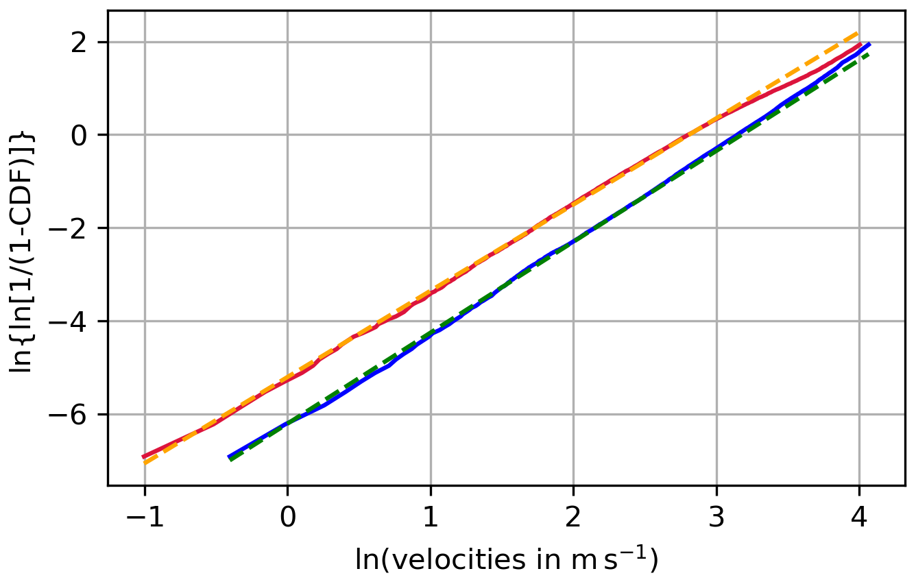
Figure C1 Cumulative distribution functions of the pseudo-velocities of ISSRs V_ISSR (red) and the wind speeds V_wind (blue) plotted on Weibull paper together with linear fits as dashed lines: g_ISSR = $\mathrm{1.85}\cdot x-\mathrm{5.2}$ (orange) and g_wind = $\mathrm{1.95}\cdot x-\mathrm{6.2}$ (green).

Appendix D: Comparison of the wind speed and direction distributions with those of other months and years

To test whether the 2 analysed months, April and May 2024, do not have exceptional wind conditions, we additionally analysed the horizontal winds on 250 hPa in the study region for 12 months from 12 years (January 2017, February 2014, March 2019, April 2022, May 2015, June 2024, July 2021, August 2018, September 2023, October 2016, November 2013, December 2020). The distribution of wind speeds is shown in Fig. D1. It shows the cumulative distribution functions (CDF) of the 2 analysed months April and May as dashed black lines plotted on a Weibull probability diagram, together with cumulative distribution functions of the selected 12 months (every fourth day, with spring in the Northern Hemisphere in green, summer in red, autumn in yellow and winter in blue). The CDFs of April and May 2024 are in the middle of the others and show no particular outliers. All lines show a very similar slope; only their intercepts differ slightly. Those of the warmer months/seasons tend to have higher intercepts than those of the colder months/seasons. The Weibull PDF (probability density function) is relatively flat if the intercept is low (higher variance, as in winter), and it gets sharper and more peaked with increasing intercept (lower variance, as in summer). Additionally, we have checked the wind roses for the 2 investigated months and the other 12 months of our test data. By and large they are similar, and there is no indication that April and May 2024 had any kind of exceptional wind distribution (speed and direction).

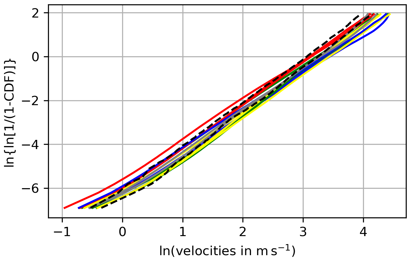
Figure D1 Cumulative distribution functions of the winds within the ISSRs of the 2 analysed months April and May 2024 as dashed black lines plotted on a Weibull probability diagram, together with cumulative distribution functions of all winds of April and May 2024 as grey lines and the winds of 12 months of 12 years, shuffled (spring in the Northern Hemisphere in green, summer in red, autumn in yellow and winter in blue).