Estimation of diurnal emissions of CO₂ from thermal power plants using spaceborne integrated path differential absorption (IPDA) lidar

Coal-fired power plants are a major source of global carbon emissions, and accurately accounting for these significant emission sources is crucial in addressing global warming. Many previous studies have used Gaussian plume models to estimate power plant emissions, but there is a gap in observation capabilities for high-latitude regions and nighttime emissions. However, large emitting power plants exist in high-latitude areas. The DQ-1 satellite is equipped with the world's first active remote sensing lidar for detecting CO₂ column concentrations, which, compared to passive remote sensing satellites, enables observations in these regions. This paper applies a two-dimensional Gaussian plume model to the XCO₂ results from the DQ-1 satellite and analyses the instantaneous CO₂ emissions of 10 power plants globally. Among these, 15 cases of data are from nighttime observations, and 3 cases are from power plants located above 60° N latitude. The estimation results show good consistency when compared with emission inventories such as Climate TRACE and Carbon Brief, with a correlation coefficient R = 0.97. The correlation coefficient between the model fits and satellite observations ranges from 0.49 to 0.88, and the overall relative random error in the estimates is 15.11 %. This paper also analyses the diurnal differences in CO₂ emissions from power plants and finds emission fluctuations directly correlated with regional electricity demand dynamics. This method is very effective for monitoring emissions from strong point sources such as power plants.

1 Introduction

Global warming is caused by the continuous increase in greenhouse gases in the atmosphere. The Kyoto Protocol under the United Nations Framework Convention on Climate Change classifies six gases, including carbon dioxide (CO₂), methane (CH₄), nitrous oxide (N₂O), hydrofluorocarbons (HFCS), perfluorocarbons (PFCS), and sulfur hexafluoride (SF₆), as major greenhouse gases, with CO₂ being the largest contributor and a key anthropogenic greenhouse gas (Kyoto Protocol, 1997). Changes in atmospheric composition due to industrial development, land-use changes, deforestation, and livestock farming have led to global warming and a series of severe events impacting the Earth's ecological environment, such as frequent natural disasters. These effects are further exacerbated by increasing greenhouse gas emissions (Arias et al., 2021; Searchinger et al., 2018). Currently, greenhouse gas emissions are accelerating, with global annual CO₂ emissions rising from 27 to 49 Pg over the past 40 years (Friedlingstein et al., 2022). In response to the severe challenges posed by climate change, countries worldwide are actively participating in CO₂ growth control initiatives and formulating strategies. China aims to peak CO₂ emissions by 2030 and achieve carbon neutrality by 2060 to curb the sharp rise in atmospheric CO₂ concentrations (Li et al., 2022).

Effective control of CO₂ emissions relies on accurate, timely, and transparent monitoring. Currently, countries assess emission reduction measures through greenhouse gas inventories, but challenges such as data lag, inconsistent standards, and insufficient information transparency undermine comparability and credibility (Tubiello et al., 2015; Peters et al., 2012). For monitoring urban CO₂ emissions, most methods employ emission models based on inventory data, following a “bottom-up” approach (Gurney et al., 2017; Turnbull et al., 2018; Lauvaux et al., 2016). In recent years, some studies have used “top-down” approaches, such as combining satellite observation data with WRF-STILT or WRF-Chem models to quantify urban greenhouse gas emissions (Turner et al., 2020; Pillai et al., 2012; Hu et al., 2022; Wu et al., 2018; Ye et al., 2020). For small point sources like power plants, airborne or ground-based monitoring is typically used to measure CO₂ concentrations. Relevant studies have employed the mass balance method to assess CO₂ emissions from power plants and cities through airborne observations (Ahn et al., 2020). Some research teams have also utilized the inverse Gaussian plume model with Methane Airborne MAPper (MAMAP) instruments to remotely sense the column-averaged dry-air mole fractions of CO₂ (XCO₂) from power plants (Krings et al., 2018, 2011). Ground-based equipment, such as portable Fourier transform spectrometers (EM27/SUN), combined with the Gaussian plume model and the cross-sectional flux method, has also been used to measure ground-level CO₂ concentrations for specific power plants and urban areas (Ohyama et al., 2021; Luther et al., 2019).

Satellite remote sensing technology holds significant potential for monitoring atmospheric CO₂ due to its capability for long-term, periodic observations on a global scale (Zhang et al., 2021). Monitoring point-source emissions using satellites is challenging. Compared to the budgeting approach for estimating point-source emissions (Amediek et al., 2017), the Gaussian plume model (GPM) is highly influenced by the precision of atmospheric background driving fields (Nassar et al., 2017; Brunner et al., 2023), it is not constrained by the spatial resolution of the model, and it is more stable and effective in modelling point-source dispersion if limited by the background wind field (Toja-Silva et al., 2017; Schwandner et al., 2017). The Orbiting Carbon Observatory-2 (OCO-2) has high measurement accuracy and stable results (Sheng et al., 2023; Crisp et al., 2017; Miller et al., 2007), and its XCO₂ product can be used in conjunction with GPM for the estimation of point-source emissions. When it passes downwind of a single point source, a significant increase in XCO₂ can be observed due to strong CO₂ emissions, and by fitting the observed XCO₂ with plume simulations, instantaneous CO₂ emissions can be quantified (Nassar et al., 2017). In recent years, a series of studies have been conducted to estimate CO₂ emissions from power plants, volcanoes, and cities based on OCO-2's XCO₂ data (Nassar et al., 2017; Guo et al., 2023; Zheng et al., 2020; Crisp et al., 2017). Nassar et al. (2021) used the Gaussian plume model to estimate CO₂ emissions and uncertainties from 20 power plants and related facilities in the USA, India, South Africa, Poland, Russia, and South Korea, noting an average difference of 15.1 % between the estimated emissions and reported values for US power plants (Nassar et al., 2021). However, OCO-2 and OCO-3 are passive remote sensing satellites, which present data gaps in high-latitude and nighttime observations, and their spatial resolution of 1.5 km × 2.25 km poses limitations for monitoring small-scale strong point sources (Shi et al., 2023; Eldering et al., 2019). For power plants, due to variations in power demand, nighttime emissions differ significantly from daytime levels, and there may be instances of illegal nighttime over-emissions at certain plants, making nighttime CO₂ emission observations necessary (Letu et al., 2014).

Spaceborne active remote sensing of CO₂ primarily employs the integrated path differential absorption (IPDA) principle (Ehret et al., 2008), enabling nighttime and high-latitude observations. Kiemle et al. (2017) discussed the ability to monitor CO₂ emissions using spaceborne lidar in combination with the plume model and a mass budget approach (Kiemle et al., 2017). Recent studies have demonstrated the feasibility of laser-based detection techniques for CO₂ emission monitoring (Menzies et al., 2014; Wolff et al., 2021). In 2022, China launched the Atmospheric Environment Monitoring Satellite (AEMS, also known as DQ-1), the first equipped with a spaceborne IPDA lidar capable of global XCO₂ measurements. This technology addresses the gap in XCO₂ observations at high latitudes and during nighttime (Cai et al., 2022; Fan et al., 2024). The XCO₂ results from DQ-1 were validated against TCCON (Total Carbon Column Observing Network) observations, showing an average deviation of less than 1 ppm at a 50 km (149 footprints averaged) resolution (Zhang et al., 2024). Additionally, its satellite footprint interval is 330 m, significantly enhancing the estimation accuracy for small power plants (Zhang et al., 2023). Han et al. (2024) applied the EMI-GATE model, based on the Gaussian plume, to evaluate power plant emissions using DQ-1 data (Han et al., 2024). The main differences between the Gaussian plume model used in this study and the EMI-GATE model used by Han et al. (2024) are the methods used to calculate the Gaussian plume model parameters such as the atmospheric instability parameters and the wind field, as well as the fact that we additionally quantify the uncertainty due to atmospheric instability. This paper also analyses 2 years of satellite data, examining emission variations in a single power plant over time. Section 2 introduces the data sources and methods of this study. In Sect. 3, the improved Gaussian plume model is integrated with DQ-1 satellite observations, selecting 10 globally high-emission power plants, including 15 nighttime observations and 23 observations of power plants in high-latitude regions, estimating their CO₂ emissions. Analyses of diurnal and seasonal variations in CO₂ emissions are also conducted. Section 4 provides a summary and discusses the potential applications of the Gaussian plume model with spaceborne IPDA lidar.

2 Data and methodology

2.1 Data

2.1.1 DQ-1 satellite data

On 16 April 2022, China launched the world's first satellite designed for the active remote sensing of carbon dioxide. This satellite is equipped with an aerosol and carbon dioxide laser detection lidar (ACDL). The primary scientific objectives are to measure high-resolution vertical profiles and the optical properties of global atmospheric aerosols and clouds, as well as to obtain global atmospheric CO₂ column concentration data. This provides precise quantitative information for studies on CO₂ sources and sinks (Fan et al., 2024). The satellite utilizes integrated path differential absorption (IPDA) technology to measure CO₂ column concentration. It employs a 1572 nm pulsed laser and the IPDA lidar method, using two wavelengths (λon and λoff, corresponding to regions of strong and weak absorption lines). The difference in absorption cross-sections (σ) between these two wavelengths is used to determine the CO₂ column concentration. XCO₂ can be calculated using these two wavelength echo signal strengths combined with the following equation (Ehret et al., 2008):

$$\begin{array}{}\text{(1)}& {\mathrm{XCO}}_{\mathrm{2}}={\displaystyle \frac{\mathrm{DAOD}}{\mathrm{IWF}}}={\displaystyle \frac{\frac{\mathrm{1}}{\mathrm{2}}\ln \frac{P_{\mathrm{off}}{E}_{\mathrm{on}}}{P_{\mathrm{on}}{E}_{\mathrm{off}}}}{{\int }_{P_{\mathrm{TOA}}}^{P_{\mathrm{G}}}\frac{\mathrm{\Delta }\mathit{\sigma }\left(p,T\right)}{\left(m_{\mathrm{dryair}}+{\mathit{\rho }}_{{\mathrm{H}}_{\mathrm{2}}\mathrm{O}}\left(p\right)m_{{\mathrm{H}}_{\mathrm{2}}\mathrm{O}}\right)g}\mathrm{d}p}}.\end{array}$$

DAOD is differential absorption optical depth, IWF is the integral weight function, P_on/P_off represents the echo power of the two laser beams, E_on/E_off represents the emitted power, p_TOA and p_G are the pressure at the top of the atmosphere and at the ground, Δσ(p,T) represents the differential absorption cross-section, m_dryair is the molecular mass of dry air, and ${\mathit{\rho }}_{{\mathrm{H}}_{\mathrm{2}}\mathrm{O}}$ is the relative humidity of the air. On-orbit tests of ACDL have yielded high-precision remote sensing data, confirming that the CO₂ column concentration measurement accuracy is better than 1 ppm. Notably, this satellite provides the first global CO₂ column concentration measurements at night and over the poles (Zhang et al., 2024). The satellite's footprint spacing of 330 m ensures high spatial resolution. This study utilizes the satellite's L2D product, which includes global XCO₂ data derived from raw observation data combined with the IPDA lidar inversion method. The datasets include XCO₂ values, uncertainty for XCO₂, and the corresponding surface elevation and geographic coordinates for each footprint.

2.1.2 Wind data

This study utilizes horizontal (U) and vertical (V) wind components from the fifth-generation European Centre for Medium-Range Weather Forecasts (ECMWF) global climate atmospheric reanalysis dataset (ERA-5). The dataset features a temporal resolution of 1 h, a spatial resolution of 0.25°, and 37 vertical pressure levels (Hersbach et al., 2020). A four-dimensional interpolation method is applied to the U and V vectors at the plume lift height, which is set to a default chimney height of 240 m and a plume vertical lift height of 250 m (Hu and Shi, 2021). To evaluate the impact of wind speed uncertainty on power plant emission predictions, the study also compares results using MERRA-2 horizontal wind data (Gelaro et al., 2017). In this study, atmospheric instability is calculated from surface 2 m wind speeds and cloud cover, with surface wind speed data selected from spatially interpolated ERA5-Land hourly wind speed U and V vectors. Additionally, the conversion of emissions into XCO₂ enhancements requires surface pressure and water vapour column content data, which were derived from ERA5-Land datasets.

2.1.3 CO₂ emissions data

The power plant validation data used in this study are sourced from the Carbon Brief database (https://www.carbonbrief.org/mapped-worlds-coal-power-plants/, last access: 12 December 2024). However, many power plants in high-latitude regions do not provide emission data. Therefore, this study also compares the results with those from Climate TRACE (https://climatetrace.org/explore/#admin=&gas=co2e&year=2024&timeframe=100&sector=power,electricity-generation&asset=​​​​​​​, last access: 30 June 2025). Climate TRACE estimates the activity levels (capacity factors) of power plants and other facilities using satellite observations and machine learning methods. The database provides annual and monthly CO₂ emissions and generating capacity for more than 500 power plants worldwide. We also compared the emissions of Climate TRACE's top 30 power plants with Carbon Brief, which had an average deviation of 9.2 %, and we considered their results to be reliable.

2.2 Emission inversion and emission uncertainties

Gaussian plume models are widely used for monitoring point-source emissions due to their stability (Brusca et al., 2016). This study applies this method to a spaceborne IPDA lidar to estimate CO₂ emissions from power plants. The basic equation of the model is as follows (Pasquill and Smith, 1983):

$$\begin{array}{}\text{(2)}& \mathrm{\Delta }Q\left(x,y\right)={\displaystyle \frac{F}{\sqrt{\mathrm{2}\mathit{\pi }}a\cdot {\left(\frac{x}{x_{\mathrm{0}}}\right)}^{\mathrm{0.894}}\mathit{\mu }}}{e}^{-\frac{\mathrm{1}}{\mathrm{2}}{\left(\frac{y}{a\cdot {\left(\frac{x}{x_{\mathrm{0}}}\right)}^{\mathrm{0.894}}}\right)}^{\mathrm{2}}},\end{array}$$

where x and y represent the distances from the chimney along the wind direction and vertical to the wind direction (m), ΔQ is the total CO₂ column increment (g m⁻²), F is the point-source CO₂ emission rate (g s⁻¹), and a is the atmospheric stability parameter which is related to the solar radiation index and surface wind speed. The solar radiation index can be assessed using high cloud cover, low cloud cover, and solar elevation angle (Pasquill, 1961; Beals, 1971). The total CO₂ column amount converted to the increment of column concentration ΔXCO₂ (ppm) can be calculated using the following equation (Zheng et al., 2020):

$$\begin{array}{}\text{(3)}& \mathrm{\Delta }{\mathrm{XCO}}_{\mathrm{2}}\left(x,y\right)=\mathrm{\Delta }Q\left(x,y\right)\cdot {\displaystyle \frac{M_{\mathrm{air}}}{M_{{\mathrm{CO}}_{\mathrm{2}}}}}\cdot {\displaystyle \frac{g}{P_{\mathrm{surf}}-w\cdot g}}\cdot \mathrm{1000},\end{array}$$

where M_air is the molecular mass of dry air (g mol⁻¹), $M_{{\mathrm{CO}}_{\mathrm{2}}}$ is the molecular mass of carbon dioxide (g mol⁻¹), g is the acceleration due to gravity, P_surf is the surface pressure (Pa), and w is the water vapour column content (kg m⁻²).

The satellite-observed XCO₂ results need to be converted into the CO₂ increment ΔXCO₂ caused by power plant emissions. The diffusion of CO₂ plumes can be simplified using a two-dimensional Gaussian model, where the footprint of the spaceborne lidar is tangent to the two-dimensional Gaussian plume, leading to a shape similar to a one-dimensional Gaussian distribution. It is assumed that the background CO₂ concentration might exhibit a small gradient linear change, and XCO₂ distribution is considered to follow the distribution

$$\begin{array}{}\text{(4)}& {\mathrm{XCO}}_{\mathrm{2}}\left(x\right)={{\mathrm{XCO}}_{\mathrm{2}}}_{\mathrm{b}}+B\cdot x+{\displaystyle \frac{A}{\mathit{\sigma }\sqrt{\mathrm{2}\mathit{\pi }}}}{e}^{\left[-(x-\mathit{\mu }{)}^{\mathrm{2}}/\mathrm{2}{\mathit{\sigma }}^{\mathrm{2}}\right]},\end{array}$$

where A, B, σ, and μ are the parameters in the linear fit function, obtained by least-squares fit; ${{\mathrm{XCO}}_{\mathrm{2}}}_{\mathrm{b}}+B\cdot x$ is the background value of XCO₂; and $\frac{A}{\mathit{\sigma }\sqrt{\mathrm{2}\mathit{\pi }}}{e}^{\left[-(x-\mathit{\mu }{)}^{\mathrm{2}}/\mathrm{2}{\mathit{\sigma }}^{\mathrm{2}}\right]}$ is ΔXCO₂ caused by power plant emissions (Reuter et al., 2019).

Figure 1 Inversion framework for Gaussian plume models.

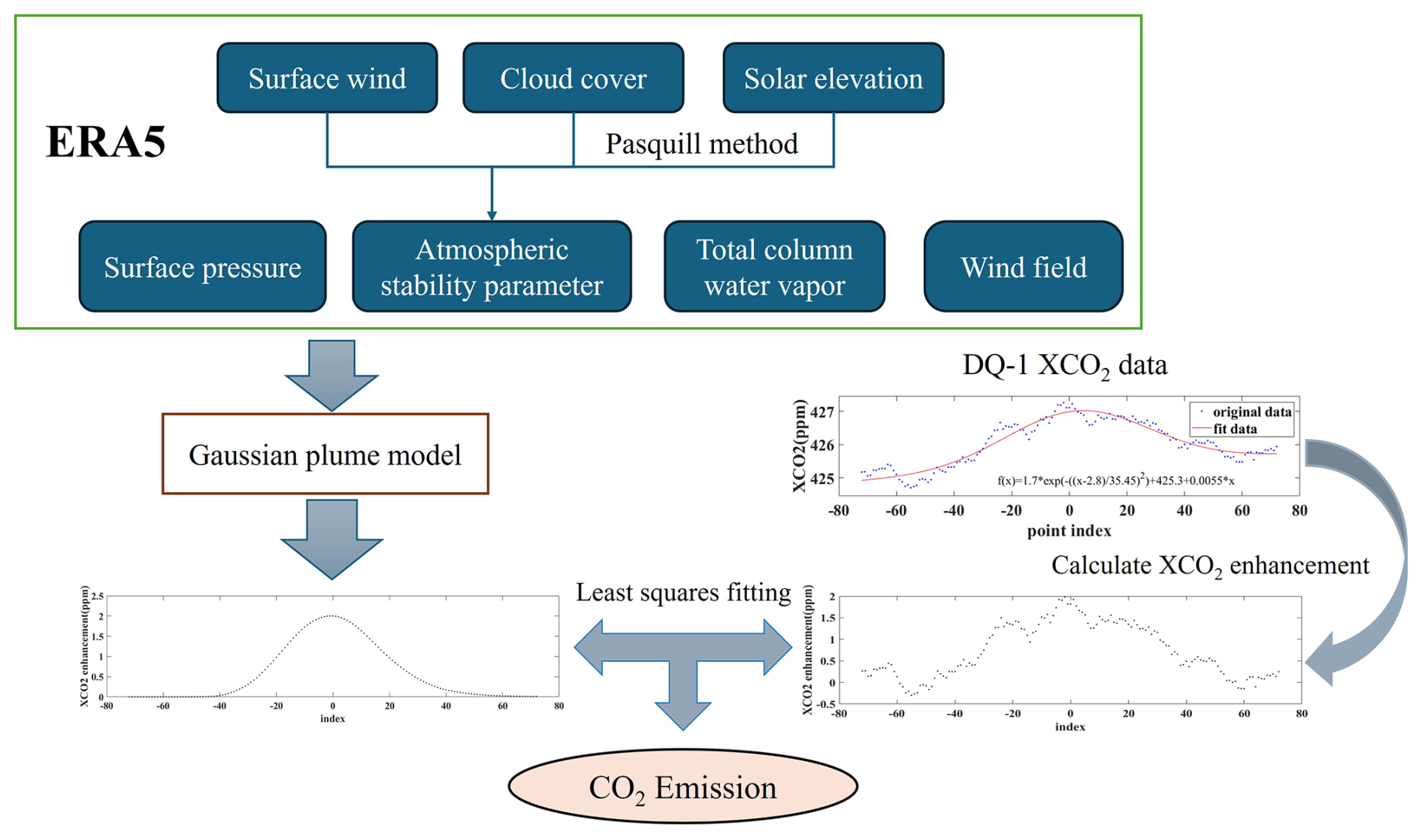
The specific calculation process is illustrated in Fig. 1. For a power plant with an emission rate of 1000 kg s⁻¹, the downwind XCO₂ enhancement at 50 km under 10 m s⁻¹ winds is < 1 ppm, which is less than the uncertainty of XCO₂ observed by the DQ-1, indicating low reliability in distant plume detection. Therefore, to improve the model's fit with satellite observation results, the selected DQ-1 orbital data require that the downwind direction of the point source intersects with the satellite footprint and that the distance between the XCO₂ enhancement location and the point source is less than 50 km. In the simulation, the x axis of the Gaussian plume represents the direction of diffusion. Most studies use interpolated wind vectors from sources like ERA-5 at the plume height as the plume's direction (Guo et al., 2023). However, in practice, wind direction may deviate and change continuously, making instantaneous wind direction insufficient for accurate plume propagation. In this model, the plume propagation direction is defined as the vector from the chimney location to the centre of the Gaussian peak. This direction is then compared with the interpolated wind direction. Only results where the wind direction difference is less than 25° are selected for further comparison and validation.

The selected satellite observation results are ultimately fitted to the model's plume results at the satellite footprint using the least-squares method to obtain the CO₂ emission rate of the target power plant. The model's results can be calculated using Eqs. (2) and (3), where the atmospheric stability parameter significantly affects the dispersion of the plume. Direct fitting with a specific value can easily lead to estimation bias. In this study, empirical interpolation of atmospheric stability parameters was implemented by accounting for surface wind speed, cloud coverage, and solar elevation angle, the latter calculated from latitude and time of observation (Nassar et al., 2021). The uncertainty in the stability parameter was quantified through the uncertainty in surface wind speed measurements. Subsequently, a least-squares fitting approach was applied under the assumption that prior estimates of atmospheric stability parameters varied within 1 standard deviation. The optimal solution was then selected as the representative atmospheric instability value for the target location. A 10 km moving average was applied to DQ-1 data, reducing the uncertainty of XCO₂ to below 1 ppm, which facilitated the detection of enhanced XCO₂ signals (Zhang et al., 2023). Therefore, during the least-squares fitting process, the model results are also smoothed similarly. The primary differences between the Gaussian plume model used in this study and the EMI-GATE model employed by Han et al. (2024) lie in the calculation methods for the atmospheric instability parameter, background CO₂ column concentration, wind speed, and wind direction. Our approach involves varying these parameters within their respective error ranges based on the original observational values, with each parameter being calculated independently to maximize the interpretability of the results.

This study estimates the uncertainty in power plant emissions using a Gaussian plume model considering five factors: uncertainty in wind speed, uncertainty in wind direction, uncertainty in plume height, uncertainty in atmospheric stability, and uncertainty in background field. The total uncertainty can be calculated using Eq. (5):

$$\begin{array}{}\text{(5)}& \mathit{\epsilon }=\sqrt{{\mathit{\epsilon }}_{\mathrm{s}}^{\mathrm{2}}+{\mathit{\epsilon }}_{\mathrm{d}}^{\mathrm{2}}+{\mathit{\epsilon }}_{\mathrm{h}}^{\mathrm{2}}+{\mathit{\epsilon }}_{\mathrm{a}}^{\mathrm{2}}+{\mathit{\epsilon }}_{\mathrm{b}}^{\mathrm{2}}},\end{array}$$

where ε_s represents the error caused by wind speed. This is estimated by comparing the CO₂ emissions from the target power plant using wind speeds interpolated from MERRA-2 and ERA-5 data with the wind speed uncertainty given by the standard deviation between the two predictions. ε_d represents the error caused by wind direction, calculated as the difference in CO₂ emissions using wind directions interpolated from ERA-5 versus the plume direction computed in this study. ε_h represents the error caused by the emission height of the power plant. The plume height is equal to the stack height plus the plume lift height (Brunner et al., 2019), and if there is no information on the stack height for a specific power plant, the default stack height is 240 m; given the uncertainty in the plume lift height, the standard deviation of the emissions for lift heights of 160, 200, 240, 280, and 320 m is used to estimate the uncertainty. ε_a represents the error induced by atmospheric instability, which is quantified using surface wind speed and net radiation index. The uncertainty in atmospheric instability is derived from the uncertainty in surface wind speed data. ε_b represents the error in calculating the CO₂ background value. This is determined by comparing the average CO₂ concentration at points upwind of the source, outside the Gaussian plume, with the background value computed using the Gaussian fitting method employed in this study, thus providing the uncertainty in the CO₂ background field.

3 Results and discussion

In this study, we utilized the DQ-1 satellite's Level 2D XCO₂ data and selected power plants with characteristics such as being located at mid-to-high latitudes and having large CO₂ emissions from Climate TRACE. A total of 97 satellite overpasses within 50 km circular regions centred on plant stacks were retrieved. For 10 typical coal-fired power plants, 47 satellite overpasses intersecting the downwind direction were identified within the power plant area. Strict data-filtering standards were applied when using the Gaussian plume model, requiring the absence of thick clouds (DQ-1 measured elevation discrepancies from DEM < 100 m) and ensuring that the deviation of the wind direction from the plume spreading direction at the point source was less than 25°. We consider that deviations of wind direction from the plume axis of less than 25° are mainly attributable to meteorological data uncertainties, while larger deviations (≥ 25°) may be due to atmospheric turbulence effects (Panofsky and Dutton, 1984), when Gaussian plume modelling is not appropriate. After filtering, 34 % of the overpasses were discarded due to excessive differences in wind direction, and a total of 28 overpasses were finally selected, including 15 nighttime cases and 3 cases when the power plant was located above 60° N.

3.1 Emissions from high-latitude power plants

Reftinskaya GRES (61.7° E, 57.1° N) is the largest solid-fuel-fired power plant in Russia, generating electricity by burning coal. The plant emits not only CO₂ and other greenhouse gases but also large amounts of SO₂, NO_x, and other pollutants, making the monitoring of its emissions highly significant. Located in Sverdlovsk Oblast, the plant has a total installed capacity of 3800 MW and produces 20×10⁹ kWh of electricity annually. Climate TRACE data show that its CO₂ emissions in 2022 were 22.7 Mt, ranking it eighth among global power plants. This plant is a major power source for the Sverdlovsk, Tyumen, Perm, and Chelyabinsk regions. The plant's Chimney No. 4, at 330 m, is one of the tallest chimneys in the world, while the heights of the other chimneys are still uncertain. Due to the plant's high latitude, around 57° N, passive remote sensing satellite data are sparse (insufficient OCO-2 overpasses were available for GPM at this plant), making it difficult to estimate. However, active remote sensing methods provide high data coverage in high-latitude regions, allowing for more accurate estimates of the plant's emissions. In this study, we retrieved 2 years of observational data from July 2022 to July 2024, identifying a total of 27 valid satellite orbits passing over the plant, as shown in Fig. 2. Based on ERA-5 wind direction data and the XCO₂ distribution, 19 valid observations were identified, covering both daytime and nighttime during autumn–winter and spring–summer. These data enable analysis of the plant's emissions over time, with typical daytime and nighttime observation results presented in Fig. 3.

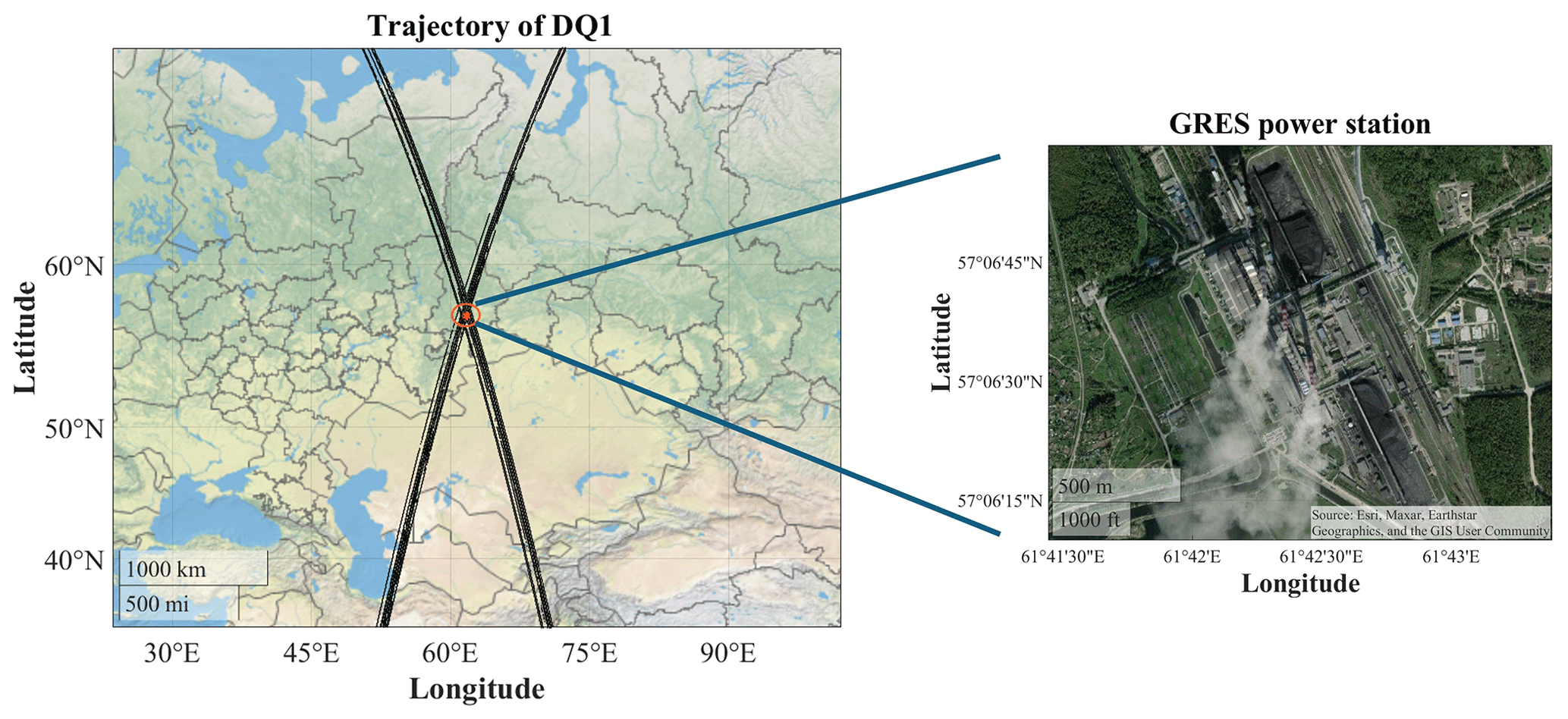
Figure 2 The DQ-1 satellite passed through all orbits around the Reftinskaya GRES power plant, where the red hexagonal star indicates the position of the power plant (map source: Esri, Maxar, Earthstar Geographics, and the GIS User Community).

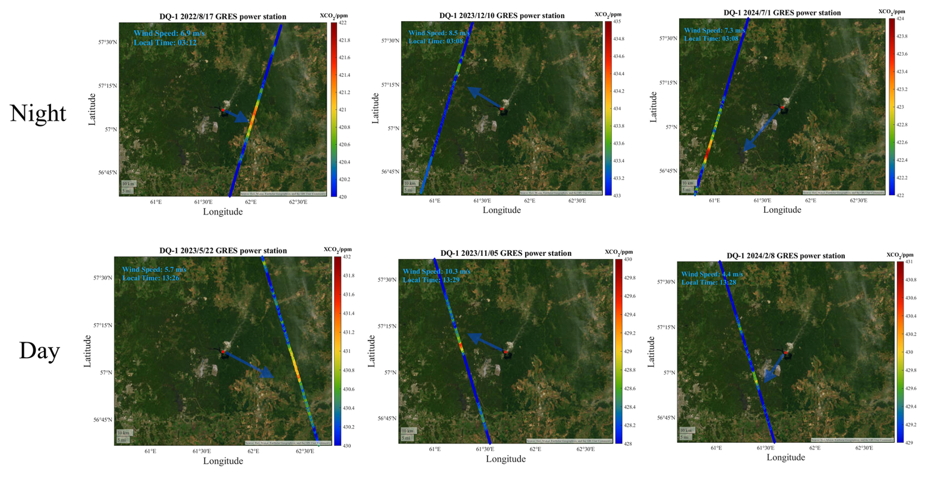
Figure 3 Typical daytime and nighttime DQ-1 overpasses around the Reftinskaya GRES power station, with the red hexagonal star indicating the location of the power station and the arrow representing the wind direction at the plume (map source: Esri, Maxar, Earthstar Geographics, and the GIS User Community).

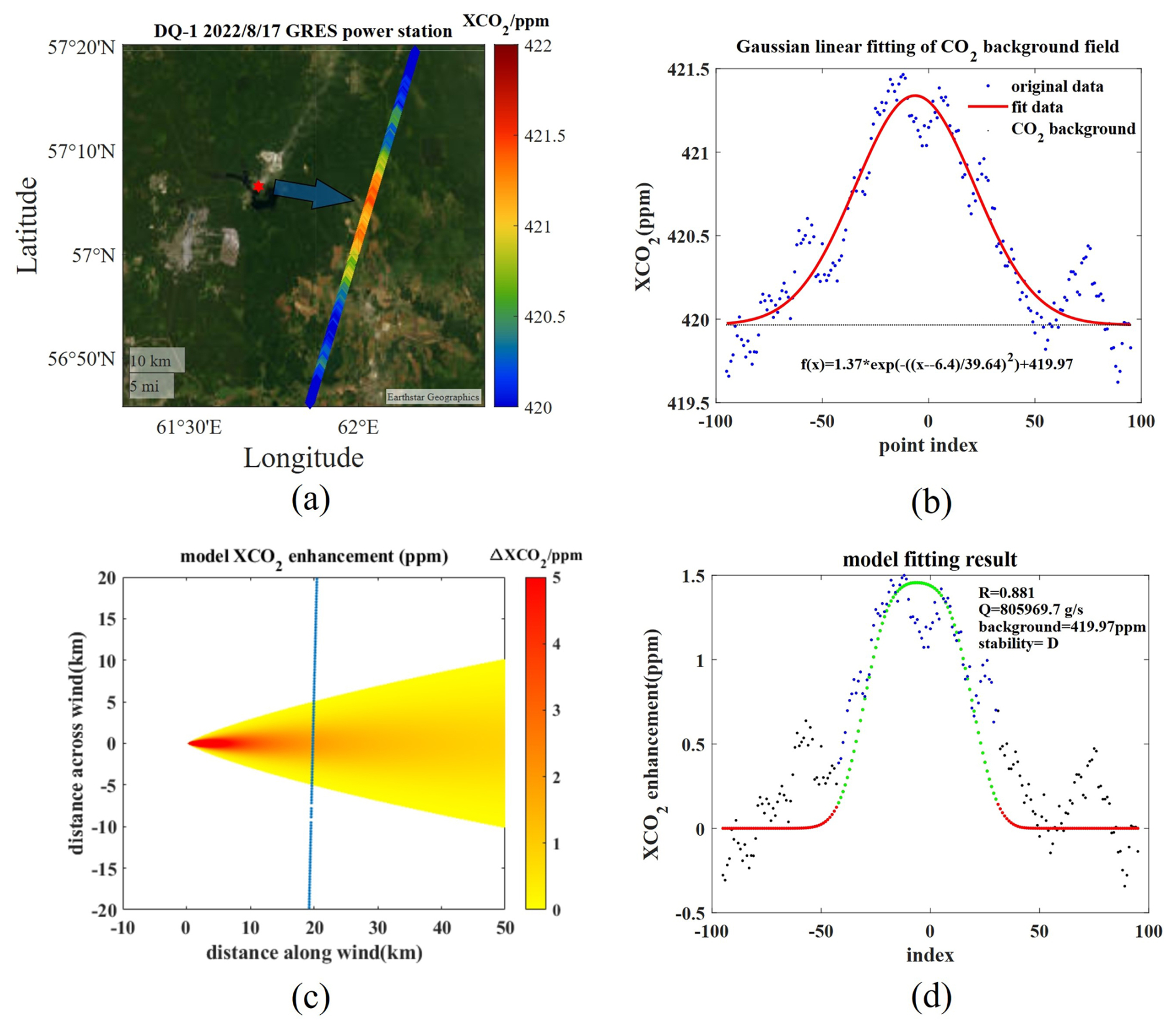
Figure 4 (a) DQ-1 satellite observation on 17 August 2022, where the red hexagonal star indicates the location of the power plant, and the red arrow indicates the result of the wind interpolation of the height of the smoke plume at that location (map source: Earthstar Geographics). (b) The result of one-dimensional linear Gaussian fitting of the satellite observation of XCO₂ results; the red line is the fitted result. (c) Gaussian plume distribution corresponding to the emission results calculated by the model; the blue point is the position of the satellite through the plume. (d) Comparison between the XCO₂ enhancement results fitted by the model and the measured results, with the red and green points indicating the model results, where the green points are the parts contained in the plume, the black and blue points are the measured results of the satellites, and the blue points are the points in the plume.

For the nighttime observation on 17 August 2022, the satellite orbit (Fig. 4a) was approximately 12 km from the power plant. Using Gaussian fitting, the background CO₂ column concentration was calculated to be 419.97 ppm, with an XCO₂ increment of about 1.3 ppm (Fig. 4b). Within the plume, there were 76 data points, assuming a plume height of 530 m above ground level (the sum of the stack height and the assumed uplift height). The CO₂ emission rate of the inventory is 721.3 kg s⁻¹. Combined with the two-dimensional Gaussian model, the theoretical XCO₂ enhancement results were calculated (as shown in Fig. 4c), and using the least-squares method, the fitted CO₂ emission result was 806.0 ± 108.2 kg s⁻¹, with a correlation coefficient of R = 0.88 (Fig. 4d). The average deviation between the model results and satellite-measured data was 0.32 ppm. The total relative error of 13.4 %, which included an uncertainty of 70.5 kg s⁻¹ due to wind conditions; 39.8 kg s⁻¹ due to background levels; and 26.1 and 64.4 kg s⁻¹ due to plume height and atmospheric stability, respectively. The slightly higher result from the model compared to the emissions inventory can be attributed to the fact that the emissions inventory represents annual averages. When converting these averages into instantaneous emission rates, the result tends to be lower than the actual instantaneous emission due to shutdowns for maintenance throughout the year. In mild summers, despite reduced nighttime electricity demand and plant output, low-load operations impair combustion efficiency, increasing fuel use per kilowatt-hour and exacerbating CO₂ emissions through frequent start–stop cycles (Hendriks, 2012).

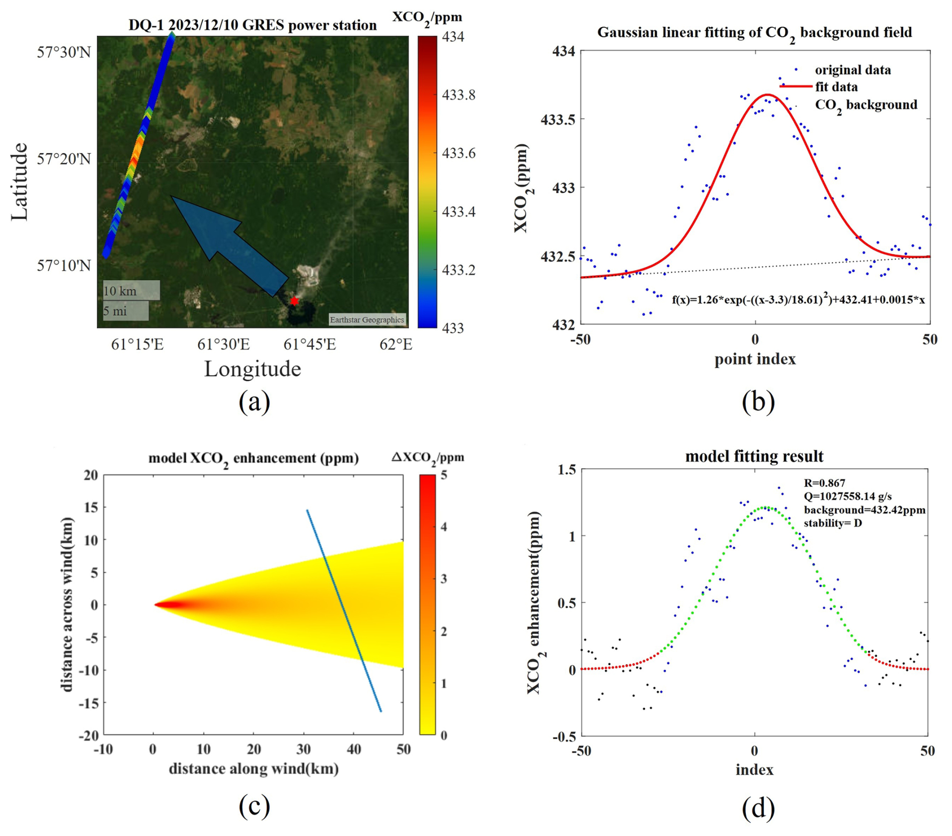
Figure 5 (a) Observations from the DQ-1 satellite on 20 December 2023 (map source: Earthstar Geographics). (b) The result after fitting the satellite observation of XCO₂ results to a one-dimensional linear Gaussian; the red line is the fitted result. (c) Gaussian plume distribution corresponding to the emission results calculated by the model. (d) Comparison of the model-fitted XCO₂ enhancement results with the observation results.

On the night of 10 December 2023, the satellite also passed over this power plant, with the corresponding satellite trajectory (Fig. 5a) located about 31 km from the plant. Using Gaussian fitting, the background value was determined to be 432.42 ppm, and the XCO₂ enhancement was 1.2 ppm. There were 57 points within the Gaussian plume, and the Gaussian plume model predicted the instantaneous emission rate of the plant to be 1027.5 ± 177 kg s⁻¹, with a correlation coefficient R = 0.87. During the error calculation, the wind speeds from ERA-5 and MERRA-2 were 6.9 and 7.8 m s⁻¹, respectively, contributing an uncertainty of 110.6 kg s⁻¹ due to wind conditions. Additionally, the atmospheric stability was calculated to be category D, leading to an emissions uncertainty of 94.4 kg s⁻¹. Considering all factors, the total relative error was 17.3 %. Since December is already winter in Russia, the increased electricity demand for city lighting, transportation, and residential heating systems (Savić et al., 2014) required the plant to maintain higher power output to meet the surrounding cities' electricity needs, leading to an increase in instantaneous emissions.

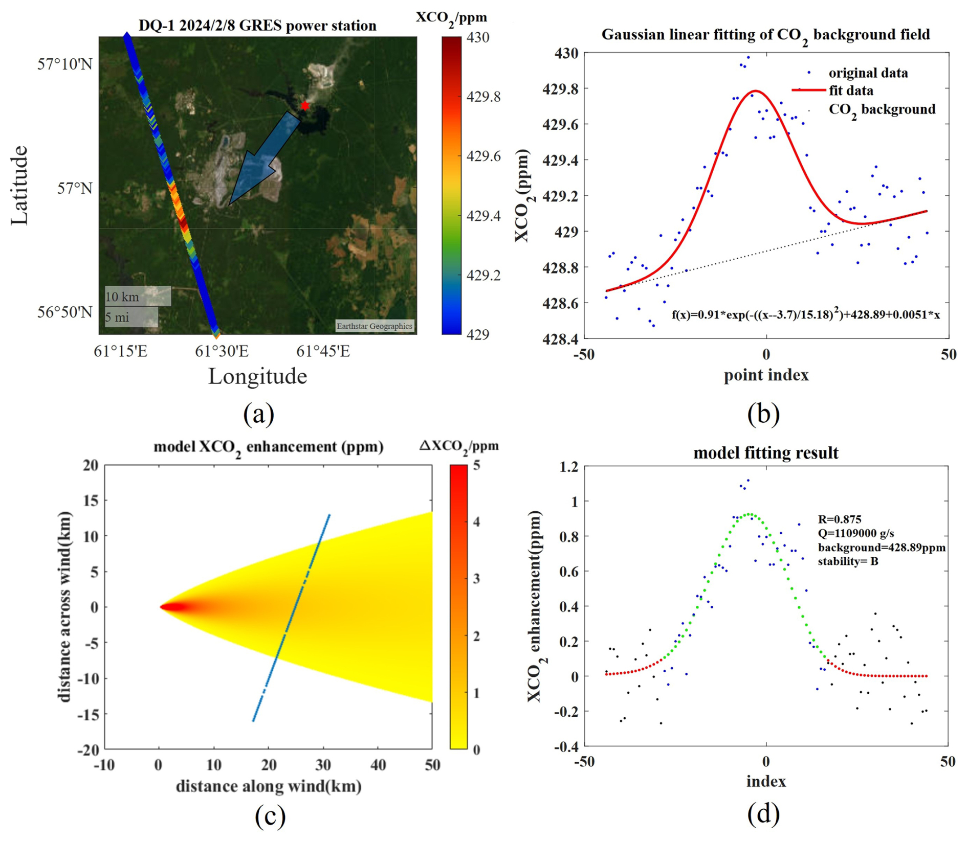
Figure 6 (a) Observations from the DQ-1 satellite on 8 February 2024 (map source: Earthstar Geographics). (b) Fitting the satellite observation of XCO₂ results to a one-dimensional linear Gaussian; the red line is the fitted result. (c) Gaussian plume distribution corresponding to the CO₂ emissions calculated by the model. (d) Comparison between the XCO₂ enhancement results fitted by the model and the measured results.

On 8 February 2024, the DQ-1 satellite passed over the power plant again during the day at 08:29 UTC (Fig. 6a), with the Gaussian plume centre located about 21 km downstream of the wind direction. In this observation, the atmospheric background field exhibited a strong linear variation trend (about 0.015 ppm km⁻¹ along the track), and the Gaussian linear fitting results are shown in Fig. 6b, with an average XCO₂ background concentration of 428.9 ppm. The surface wind speed was 4.2 m s⁻¹, and the atmospheric stability was calculated to be class B. There were 51 points within the plume. Using the Gaussian plume model, the plant's instantaneous emission rate was predicted to be 1109 ± 169 kg s⁻¹, with a correlation coefficient R = 0.875 between the model results and satellite observations. The total uncertainty in the estimated emission rates was 168.9 kg s⁻¹, with a relative error of 15.3 %. The largest contribution to this uncertainty was from the variation in the CO₂ background field, which caused an emission calculation uncertainty of 109.3 kg s⁻¹. The uncertainties due to wind field, plume height, and atmospheric stability were 88.9, 31.5, and 85.4 kg s⁻¹, respectively. Compared to the observation in December, the CO₂ emissions were higher in this February observation, which can be attributed to the fact that the observation was conducted during the day when electricity demand is higher due to residents' work activities, leading the power plant to increase output, thereby raising CO₂ emissions (Waite et al., 2017).

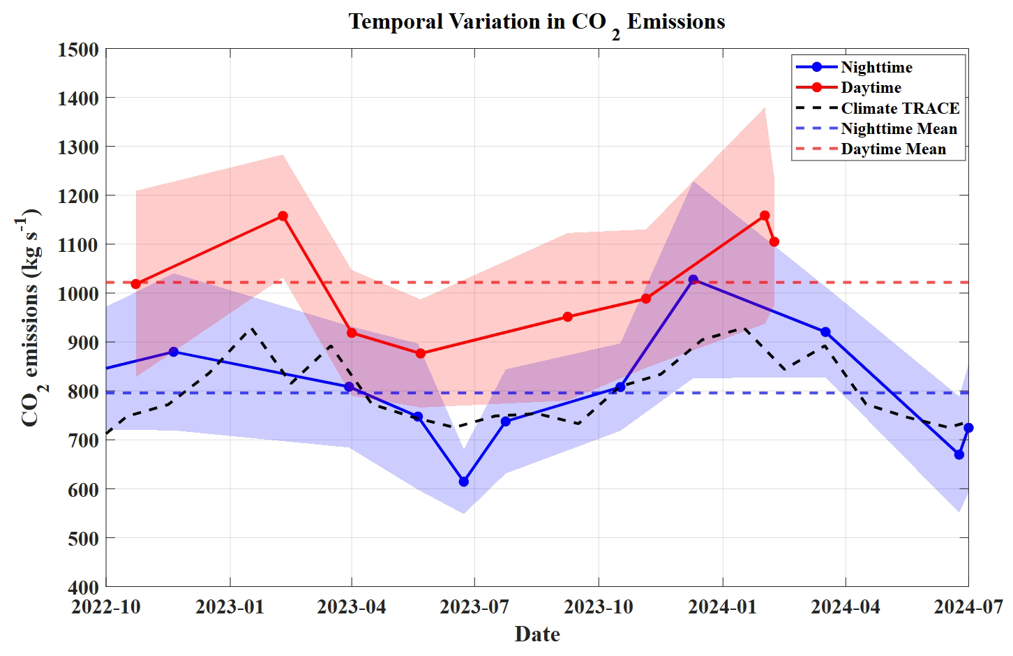
Figure 7 Daytime (red) and nighttime (blue) CO₂ emission rates from GRES power plants (2022–2024). Solid lines represent modelled estimates with uncertainty bounds (shaded areas), dashed red and blue lines represent average daytime and nighttime emissions, and dashed black lines represent Climate TRACE emission inventory values.

By analysing 2 years of observation data from the GRES power plant (as shown in Fig. 7 and Table 1), the overall estimated average emission rate is higher than the emissions reported in the inventory. The plant undergoes annual shutdowns for maintenance, and the satellite observations represent instantaneous emissions, which may differ slightly from the annual average emissions. Additionally, the Climate TRACE data reflect the 2022 annual average emissions, and the plant's yearly emissions fluctuate due to varying local electricity demand. Figure 7 shows that summer emissions are lower than winter emissions. It was found that the plant is located in a high-latitude region where the climate is mild in summer and cold in winter. During winter, residents use electrical appliances and heating systems more frequently, and the power demand for urban infrastructure is higher than in summer. As a result, the power plant adjusts its output, leading to higher CO₂ emissions in winter (Savić et al., 2014). The comparison between daytime and nighttime observations shows that the average CO₂ emission rate during the day is 1022 kg s⁻¹, while the nighttime average is 796 kg s⁻¹. The ratio of daytime to nighttime emission rates is 1.28. This ratio can be used to estimate the full-day CO₂ emissions when only daytime or nighttime observations are available. The power plant is the primary source of electricity for the region, and electricity demand from production activities during the day is much higher than at night. Consequently, the plant increases its load during the day, resulting in higher CO₂ emissions. This also indicates that the plant does not engage in unauthorized nighttime emissions during the observation period.

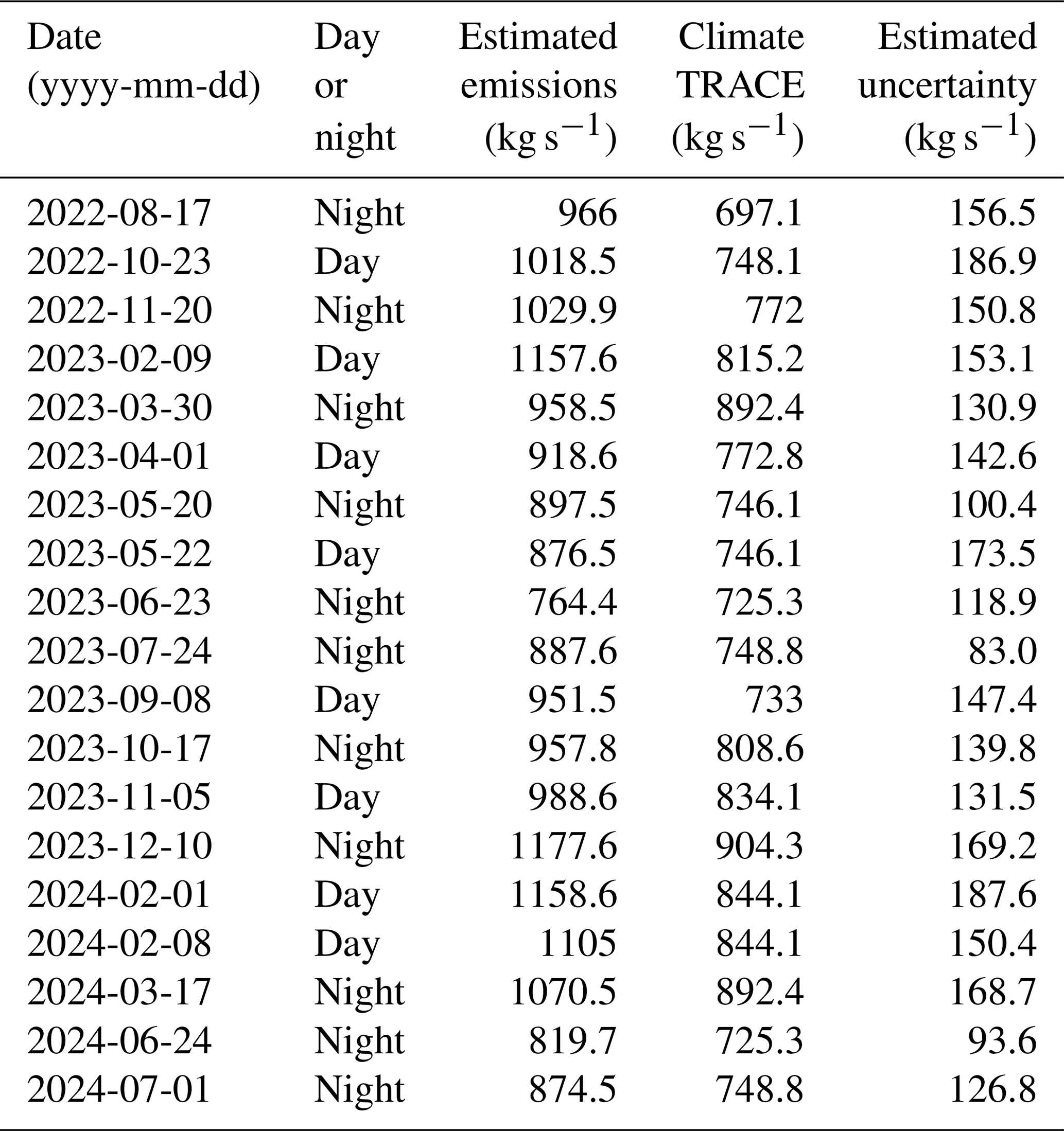
Table 1 Emission estimates and uncertainty for GRES power plant.

3.2 Comparison with emission inventories

The estimations from this study were compared with the emission inventories provided by Climate TRACE and Carbon Brief, as shown in Table 2. Both inventories present the annual total emission values, whereas the model results calculated from satellite observations represent instantaneous emission rates. Due to the power plant's ability to adjust its output based on local electricity demand, some differences between the two sets of results are expected. However, most results fall within the error range of the model predictions. The study includes three observation cases for latitudes above 60° N and 15 cases of nighttime emission detections. The use of spaceborne lidar to detect XCO₂ effectively compensates for the limitations of passive remote sensing satellites in high-latitude and nighttime observations. A comparison of all observation results with the Climate TRACE inventory is shown in Fig. 8, with a correlation coefficient of 0.97.

Table 2 Information on different power plants and the comparison of model predictions with emission inventories.

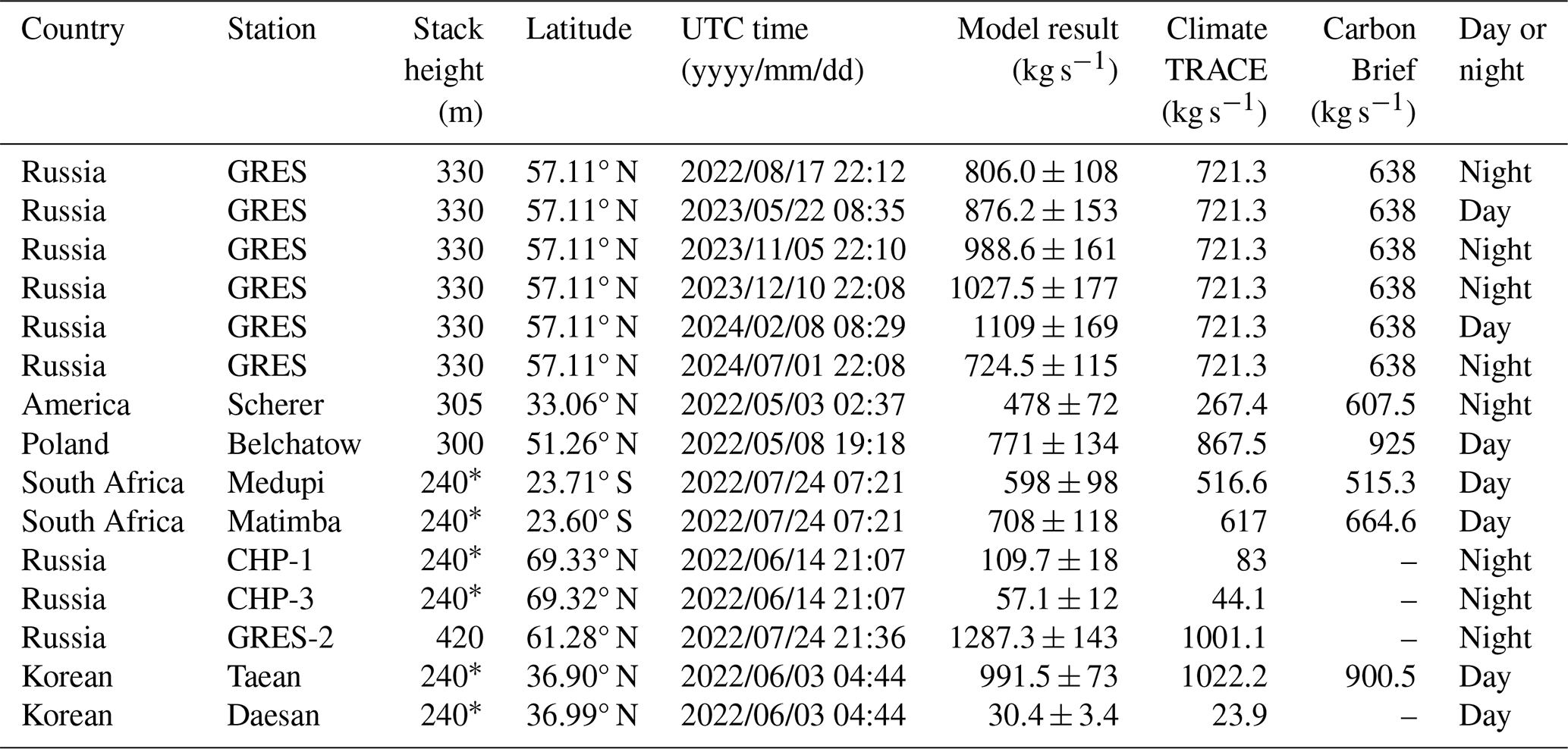
^∗ The default stack height is 240 m (Nassar et al., 2021).

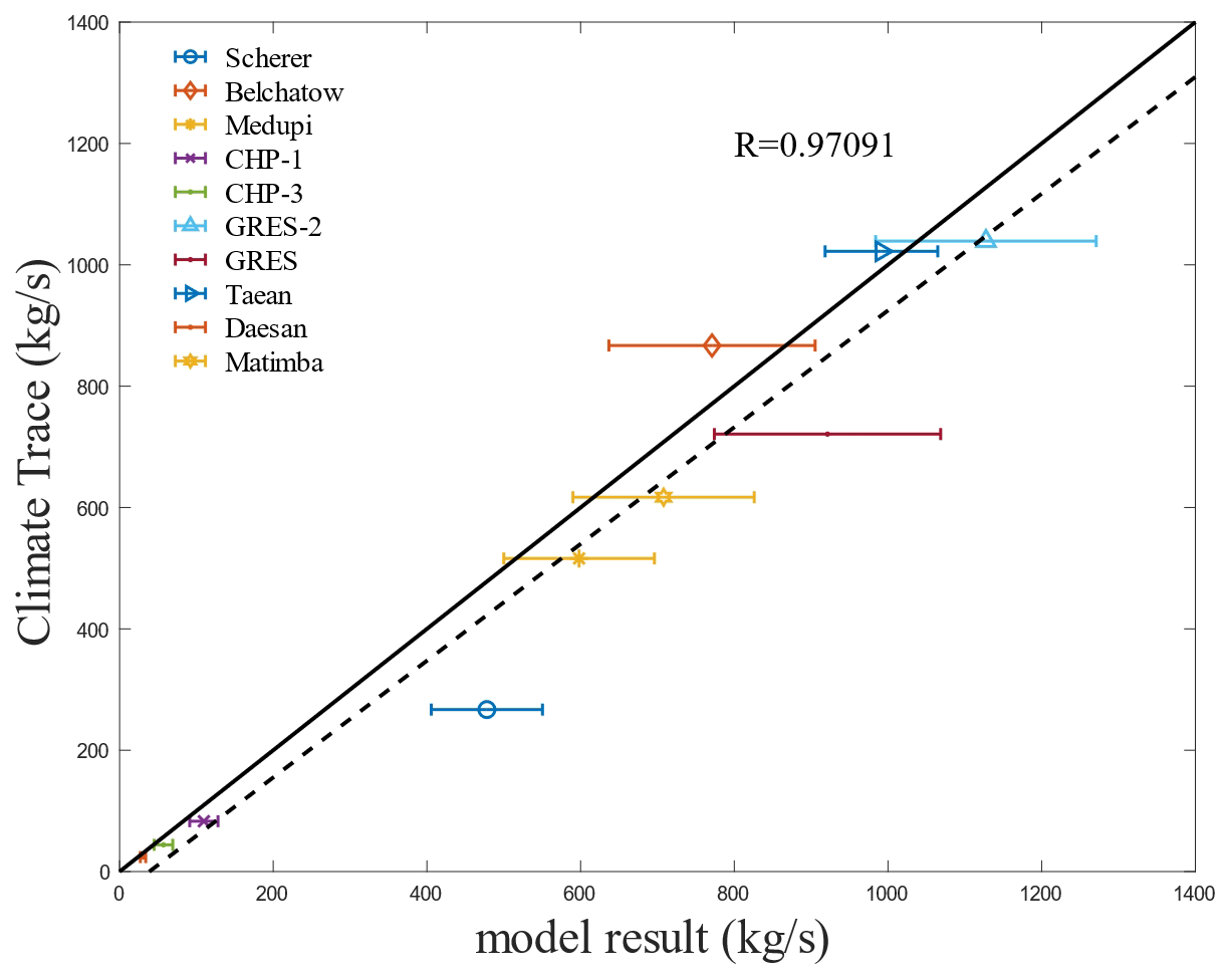
Figure 8 Comparison of power plant emissions predicted by Gaussian plume model with Climate TRACE statistics; the solid black line represents the 1 : 1 line, and the dashed line indicates the linear fitting line.

Overall, the CO₂ emissions predicted by the Gaussian plume model are generally higher than those in the emissions inventory. This discrepancy may be due to the timing of observations, as some were conducted during winter and summer in the Northern Hemisphere when increased electricity demand prompts power plants to elevate generation capacity. Comparisons between nighttime and daytime CO₂ emissions reveal lower nighttime emissions at some plants, potentially attributable to reduced electricity demand (Waite et al., 2017) and real-time adjustments to avoid power storage saturation. However, nighttime emissions at certain plants exceed inventory values, which could result from suboptimal equipment load levels reducing overall efficiency and causing incomplete fuel combustion. Additionally, frequent start–stop operations during low-load conditions may contribute to unstable combustion, further amplifying emissions (Hendriks, 2012). Overall, the emission rates measured in this study exceed those reported by Carbon Brief and Climate TRACE, a difference that might arise because conventional power plants undergo annual shutdowns for inspections, lowering annual averages relative to instantaneous emissions. It is critical to acknowledge that direct validation against stack monitor measurements is unavailable, and emission inventories are inherently uncertain and not independently validated. Therefore, comparisons between estimated results and inventories should be interpreted cautiously and serve as a provisional reference rather than definitive conclusions. Moreover, by utilizing the high spatial resolution of the DQ-1 satellite, it is possible to monitor low-CO₂-emitting power plants (F < 100 kg s⁻¹), with results fitting well with the inventory data.

3.3 Emissions uncertainty analysis

The uncertainty in the model calculations was assessed using Eq. (5) from Sect. 2.2, revealing that the uncertainty contributions vary across different power plants and influencing factors. The overall uncertainty results are presented in Table 3. The average relative random error is 15.11 %, which is lower than the 18.8 % random error in the EMI-GATE model (Han et al., 2024). The primary contributors to this uncertainty are errors in the background field calculation, wind field errors, and atmospheric stability errors. Regarding wind fields, both the ERA-5 and MERRA-2 datasets are reanalysis results. However, discrepancies can occur between these datasets, particularly in high-latitude regions where wind speed observations are sparse. When these wind speeds are used in the Gaussian model to estimate power plant emissions, differences can lead to errors in Gaussian diffusion velocity, thereby affecting prediction accuracy (Nassar et al., 2021). In this study, wind-field-related uncertainty accounts for 26.7 % of the total error, with an average relative random error of 7.4 %. Atmospheric stability is another significant factor contributing to uncertainty. Atmospheric stability is not constant and varies in real time with solar radiation, which is influenced by factors such as cloud cover and solar elevation angle (Ashrafi and Hoshyaripour, 2010). Since atmospheric stability directly impacts the shape of Gaussian diffusion, it introduces errors in predicted CO₂ emissions. For all results considered, uncertainty due to atmospheric stability contributes 25.1 % to the total error, with an average relative random error of 7.3 %. Plume height uncertainty also plays a role in the overall error. While some power plants provide chimney height data, allowing for the consideration of plume rise uncertainty only, others require an assumed chimney height (Guo et al., 2023). This assumption can lead to relatively high errors, primarily because wind speed and direction near the ground can vary with height, resulting in inaccuracies in wind field calculations. Plume height uncertainty contributes 6.5 % to the total error, with an average relative random error of 3.3 %. Uncertainty in the background field is mainly due to inaccuracies in its calculation. In areas with significant anthropogenic interference, a linear function may not adequately represent changes in background CO₂ concentration. Additionally, satellite observations are subject to inherent errors, and uncertainties in XCO₂ retrievals can introduce errors into point-source emission estimation. Background field errors account for 40.7 % of the total error, with an average relative random error of 9.5 %. For spaceborne lidar, the spatial distribution of satellite nadir points differs from that of passive remote sensing satellites, leading to fewer observed points within the plume. This increases the weight of background field uncertainty in the total error (Nassar et al., 2021; Shi et al., 2023). The uncertainty of XCO₂ around the studied power plants is less than 1 ppm by moving average, but the average relative error in XCO₂ enhancement at the peak of the plume is as high as 47.3 %. Compared to the statistical uncertainties reported in Han et al. (2024), both investigations identified that uncertainties in the DQ-1 satellite's XCO₂ observations dominate the error budget, accounting for approximately 50 % of the total error. Beyond this, the significant contribution of wind field uncertainties aligns with findings from Nassar et al. (2017; Guo et al., 2023). In contrast to previous studies, this work incorporates uncertainties in atmospheric instability. Due to the influence of turbulence and other factors within the boundary layer, the uncertainty in surface wind speed also exerts a significant influence on atmospheric instability calculations.

Table 3 Uncertainty caused by different error factors in the forecast results of different power plants.

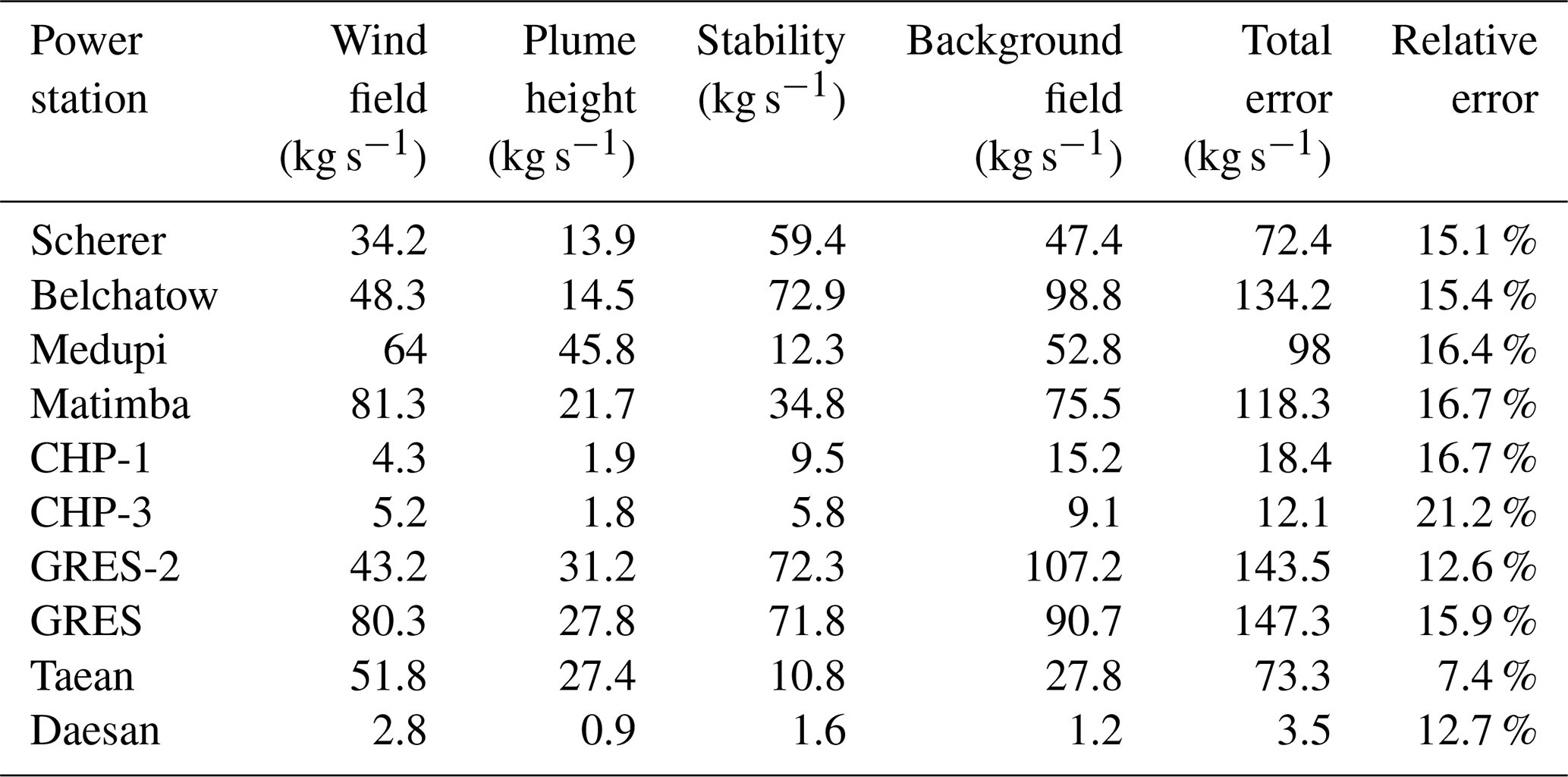
Unlike prior studies, this research explicitly accounts for atmospheric instability uncertainty. Surface wind speed uncertainty, influenced by boundary layer turbulence and other factors, is significantly higher during daytime. Our analysis of 28 cases reveals that the optimized atmospheric instability parameter a shows average deviations of 19.5 % from its prior value in daytime versus 15.8 % at night. The results indicate that, under the assumption that plume dispersion aligns with the Gaussian plume model, ERA-5 surface wind speeds exhibit higher accuracy at night. However, daytime turbulence introduces small-scale wind field errors, which further amplify uncertainties in atmospheric instability.

4 Conclusions

This study utilized the IPDA lidar on board the DQ-1 satellite to monitor emissions from localized strong point sources and, for the first time, observed the diurnal variation in CO₂ emissions from a high-latitude power plant, effectively covering areas that passive remote sensing satellites fail to monitor. The two-dimensional Gaussian plume model was optimized in terms of plume direction and atmospheric stability and applied to XCO₂ observation results. Validation and comparison results indicate that the improved Gaussian plume model has a strong correlation with the emissions inventory, with a correlation coefficient of 0.97. The average relative random error in the predicted results is 15.11 %, which is lower than that of the EMI-GATE model, due to different parameter selections in the Gaussian plume model, thus reducing the random error. The main factors affecting estimation errors are the uncertainty in the atmospheric wind field (26.7 % of total error), uncertainty in atmospheric stability (25.1 %), and uncertainty in background field calculations (40.7 %). The results show that during the daytime, the error in the surface wind field is higher due to turbulence, which can cause some invalid observations or increase the error caused by atmospheric instability and wind field to the model. Utilizing high-resolution wind fields simulated by the WRF-LES model around power plants to drive the Gaussian plume model may reduce uncertainties in the wind field. Establishing automatic weather stations around the power plant for real-time monitoring of atmospheric radiation and surface wind speed could reduce errors caused by uncertainties in atmospheric stability. Overall, power plant CO₂ emissions were largely consistent with local electricity consumption patterns, with most plants emitting less at night than during the day, and with higher emissions in winter and summer compared to spring and autumn. This research provides a new approach for global carbon accounting. In 2025, China plans to launch the DQ-2 satellite, equipped with the same IPDA lidar for carbon dioxide observation. As satellite density increases, global coverage of emission detection data will significantly improve.