Tracking daily NO_x emissions from an urban agglomeration based on TROPOMI NO₂ and a local ensemble transform Kalman filter

Accurate, timely, and high-resolution NO_x emissions are essential for formulating pollution control strategies and improving the accuracy of air quality modeling at fine scales. Since late 2018, the Tropospheric Monitoring Instrument (TROPOMI) aboard the Sentinel-5 Precursor (S5P) satellite has been providing daily monitoring of NO₂ column concentrations with global coverage and a small footprint of 5.5 km × 3.5 km, offering great potential for tracking daily high-resolution NO_x emissions. In this study, we develop a data assimilation and emission inversion framework that couples an ensemble Kalman filter with the Community Multiscale Air Quality (CMAQ) model to estimate daily NO_x emissions at 3 km scales in Beijing and surrounding areas in 2020. By assimilating the TROPOMI NO₂ tropospheric vertical column densities (TVCDs) and taking the bottom-up inventory as prior emissions, we produce a posterior NO_x emission dataset with a reasonable spatial distribution and daily variations at the 3 km scale. The proxy-based bottom-up emission mapping method at fine scales overestimates NO_x emissions in densely populated urban areas, whereas our posterior emissions improve this mapping by reducing the overestimation of urban emissions and increasing emissions in rural areas. The posterior NO_x emissions show considerable seasonal variations and provide a more timely insight into NO_x emission fluctuations, such as those caused by the COVID-19 lockdown measures. Evaluations using the TROPOMI NO₂ column retrievals and ground-based observations demonstrate that the posterior emissions substantially improve the accuracy of 3 km CMAQ simulations of the NO₂ TVCDs as well as the daily surface NO₂ and O₃ concentrations in 2020. However, during summer, despite notable improvements in surface NO₂ and O₃ simulations, positive biases in the posterior model simulations persist, indicating weaker constraints on surface emissions from satellite NO₂ column retrievals in summer. The posterior daily emissions on the 3 km scale estimated by our inversion system not only provide insights into the fine-scale emission dynamic patterns but also improve air quality modeling on the kilometer scale.

1 Introduction

As crucial atmospheric pollutants, nitrogen oxides (NO_x= NO + NO₂) play a vital role in tropospheric chemistry. NO_x acts as an important precursor to ozone and secondary inorganic aerosols, which pose risks to the ecosystem and human health. NO_x is primarily emitted into the atmosphere through anthropogenic sources such as industrial processes, transportation, and power generation (Li et al., 2017) as well as natural processes, including soil emissions, lightning, and biomass burning. Accurate and up-to-date NO_x emissions are of significant importance to formulating pollution control strategies and improving the precision of air quality simulations.

Bottom-up emission inventories are used to characterize the spatiotemporal distribution of emissions and serve as the foundational input data for atmospheric chemical transport models (CTMs). Bottom-up approaches rely on activity data and average emission factors for each source sector, which could introduce uncertainties due to incomplete statistical data and misrepresentation of emission factors. Additionally, due to the delayed availability of activity data, bottom-up inventories typically exhibit a temporal latency and cannot represent emissions accurately at the time of occurrence (Streets et al., 2003). Besides, bottom-up emission inventories typically allocate regional total emissions into fine-scale grids based on spatial proxies such as population densities, nighttime lights, road networks, and industrial gross domestic product (GDP) (Streets et al., 2003; Zhang et al., 2009; Geng et al., 2017). Such a proxy-based method assumes that emissions and spatial proxies are linearly correlated in space, which introduces biases at fine spatial scales (Wu et al., 2021). For instance, studies have shown that proxy-based emission inventories tend to overestimate emissions in densely populated urban areas and underestimate emissions in suburban and rural areas, thus propagating uncertainties to high-resolution CTM simulations (Zheng et al., 2021b).

To improve NO_x emission inventories, top-down approaches that derive NO_x emissions from NO₂ observations have been developed and widely employed in literature to account for emission spatiotemporal variations (Streets et al., 2013; Martin et al., 2003; Miyazaki et al., 2017; Mijling and van der A, 2012; Ding et al., 2015; Kong et al., 2019), especially regarding socioeconomic events such as the substantial emission fluctuations induced by COVID-19 lockdowns (Ding et al., 2020; Miyazaki et al., 2020a; Kang et al., 2022; Feng et al., 2020; Zheng et al., 2020). The mass-balance-based inversion method and its variants, which assume a direct linear relationship between local NO_x emissions and NO₂ tropospheric columns (Martin et al., 2003), or between changes in NO_x emissions and changes in NO₂ columns (Lamsal et al., 2011), have been widely adopted to infer regional NO_x emissions from satellite NO₂ retrievals (Zheng et al., 2020; Zhao and Wang, 2009; Zhu et al., 2022; Cooper et al., 2017). Although this method is suitable for short-lived gases and performs well at a coarse model resolution of tens of kilometers, the insufficient consideration of atmospheric transport between model grids and the nonlinear chemistry within each grid could cause emission-smearing errors (Cooper et al., 2017; Streets et al., 2013), particularly at fine scales.

The data assimilation technique is an alternate inversion method that works appropriately at fine spatial resolutions. The two common assimilation algorithms used for NO_x emission inversion are four-dimensional variational assimilation (4D-Var) (Cooper et al., 2020; Wang et al., 2020; Qu et al., 2017, 2019) and ensemble Kalman filter (EnKF) (Miyazaki et al., 2020b). The target parameters (i.e., emissions) are optimized during data assimilation to minimize the discrepancy between model-predicted and observed pollutant concentrations. Atmospheric transport is accounted for by considering observations from the surrounding areas and their response to the target grid's emissions, and complicated atmospheric chemistry is incorporated into the model. Such methods are not limited to short-lived species like NO_x and are also effective for long-lived gases such as CO₂ and CH₄ (Kong et al., 2022; Liu et al., 2021; Pendergrass et al., 2023). However, due to the complex chemical simulation processes combined with the assimilation framework configurations, which require huge computational resources, studies on NO_x inversions are often limited to short periods, monthly emission inversions, or coarse grid resolutions.

The Sentinel-5P Tropospheric Monitoring Instrument (TROPOMI), launched in October 2017, provides daily global coverage with a high-resolution footprint of 3.5 × 5.5 km² (7 × 3.5 km² before 6 August 2019) and a high signal-to-noise ratio. Despite low biases in early versions of TROPOMI NO₂ data (i.e., v1.2.x and v1.3.x) (Verhoelst et al., 2021; Lambert et al., 2021), the quality of satellite data has been improved through regular data validation and retrieval algorithm improvements, including a major update in the FRESCO cloud retrieval and other algorithm updates (van Geffen et al., 2022). TROPOMI provides global detailed NO₂ observations on a near-daily basis, which have been used extensively in emission inversion across spatial scales (van Geffen et al., 2022; Douros et al., 2023). In TROPOMI-based emission inversion studies, the primary focus is on point sources or the total emissions from cities (Beirle et al., 2019; Wu et al., 2021; Lorente et al., 2019; Goldberg et al., 2019; Zhang et al., 2023). Recently, TROPOMI NO₂ retrievals have also been used to monitor emission reductions during the COVID-19 lockdowns (Zheng et al., 2020; Ding et al., 2020; Miyazaki et al., 2020a; Kang et al., 2022). These studies mainly focused on the early months of 2020 with a spatial resolution greater than several tens of kilometers, which is notably coarser than the fine footprint of TROPOMI. Furthermore, improvements to the model simulations are rarely considered in these studies.

By now, there is limited research on daily high-resolution anthropogenic NO_x emission inversion using TROPOMI retrievals, and there are very few reports on improving CTM simulations at the kilometer scale through NO_x emission inversions. Herein, our study focuses on the daily anthropogenic NO_x emission inversion at a 3 km resolution, which is close to the size of the TROPOMI pixel size, through an advanced data assimilation framework that couples an ensemble Kalman filter (EnKF) with the Community Multiscale Air Quality (CMAQ) nested model. The main objective of this study is to understand the spatial distribution patterns and the daily variations in anthropogenic NO_x emissions at fine spatial resolutions, providing insights into the evaluation of the spatiotemporal distribution of bottom-up emission inventories. The models, data inputs, and observations used for the evaluations are detailed in Sect. 2. In Sect. 3, we analyze and evaluate the emission inversion results. Section 4 discusses inversion sensitivities and uncertainties. In Sect. 5, we provide a summary of the findings from this study.

2 Data and method

The emission inversion system framework (Fig. 1) is similar to our previous study for carbon flux inversion (Kong et al., 2022). In contrast to that study, which focused on a global scale, this research utilizes the regional CMAQ model for emission inversion at daily 3 km scales based on high-resolution TROPOMI satellite NO₂ retrievals. The CMAQ model settings, satellite observation constraints, and system configurations, as well as evaluation data, are described in Sect. 2.1–2.6.

Figure 1 Flowchart of the emission inversion system.

2.1 CMAQ model and a priori emissions

In the NO_x inversion system, we used the CMAQv5.2.1 model to establish the relationship between emissions and simulated NO₂ concentrations. The meteorological fields that drive the CMAQ model are provided by the Weather Research and Forecasting (WRF) model version 3.9.1. The initial and boundary conditions for WRF are derived from the National Centers for Environmental Prediction Final Analysis (NCEP-FNL) reanalysis data. The parameterization schemes for the WRF and CMAQ models are consistent with previous studies (Cheng et al., 2019; Zhang et al., 2019; Geng et al., 2021). For the CMAQ chemical schemes, we used CB05 as the gas-phase chemical mechanism and AERO6 as the particulate matter chemical mechanism. CMAQ has 28 vertical levels in simulation, which are collapsed from the 46 sigma levels of the WRF model.

The target region of this study is the city of Beijing and its surrounding areas, which are highly susceptible to air pollution due to substantial anthropogenic emissions. To perform high-resolution simulations in this region, we designed three nested domains for the CMAQ model (Fig. S1 in the Supplement). The first domain (D01) covers China and parts of surrounding countries with a horizontal resolution of 27 km × 27 km; the second domain (D02) includes parts of northern and eastern China with a horizontal resolution of 9 km × 9 km; and the third domain (D03) covers Beijing city and its surrounding regions, including Tianjin and parts of Hebei Province, with a horizontal resolution of 3 km × 3 km. Since only the third domain is the target area for the emission inversion, the simulations over the first and second domains were performed before the inversion experiments to provide boundary conditions for the third domain. Since the inner nested domain is less influenced by the chemical processes outside the first domain, the default background profiles are used as the boundary conditions for the D01 domain. In principle, performing assimilation inversion for the D02 region first and using the posterior simulated concentrations as boundary conditions for the D03 region would reduce boundary field errors and improve emission inversion results near the D03 boundary. However, in this study, we made a trade-off between minimizing computational resources and optimizing the boundary field, ultimately performing assimilation inversion only for the D03 region.

Anthropogenic emissions for mainland China in 2020 are obtained from the Multiresolution Emission Inventory in China (MEIC, http://meicmodel.org/, last access: 20 January 2024) (Zheng et al., 2018; Li et al., 2017), which is dynamically updated using a bottom-up approach based on near-real-time activity indicators (Zheng et al., 2021a). The MEIC emission inventory is spatially and temporally allocated to match the CMAQ model domain using spatial proxies and empirical temporal profiles. Emissions from the regions outside mainland China are obtained from the MIX emission inventory (Li et al., 2017), which is coupled with the MEIC emission inventory over the first domain. The spatial proxies include total population density, urban population density, rural population density, and road length. These spatial proxies are updated annually to reflect interannual changes. The temporal profiles are unique for each major emission source. The monthly profiles capture both seasonal variations and interannual trends in emissions, reflecting real activity levels. The allocation from monthly to daily values is achieved using sector-specific profiles that incorporate weekly and workday variations. In the CMAQ model, the MEIC inventory is mapped to the CMAQ model grids. Emissions from point sources are directly assigned to the grid cells where they are located, while emissions from area sources are first allocated to 1 km × 1 km grid cells based on the spatial proxies and then aggregated to the model grids based on WRF-CMAQ grid parameters. The biogenic emissions are dynamically generated by the Model of Emissions of Gases and Aerosols from Nature (MEGAN v2.1.4), which is driven by the WRF model over the same CMAQ domains.

2.2 TROPOMI NO₂ retrievals

TROPOMI is an advanced spectrometer on board the European Space Agency's (ESA's) Sentinel 5 Precursor (S5P) satellite, with the Equator crossing time at approximately 13:30 local time (LT). TROPOMI provides measurements in a wide spectral range covering ultraviolet, visible, and shortwave infrared wavelengths, and the visible band (400–496 nm) is used for the NO₂ retrievals. TROPOMI has great advantages in monitoring and inferring trace gas emissions at fine spatial scales, as it provides near-daily global coverage with a wide swath of 2600 km, and an unprecedented high-resolution footprint. A negative bias was identified in early versions of the TROPOMI NO₂ data (i.e., v1.2.x and v1.3.x), particularly in polluted regions, compared to ground-based or OMI (the ozone monitoring instrument) measurements (Verhoelst et al., 2021; Lambert et al., 2021). With a major update in the FRESCO cloud retrieval and other algorithm updates including an adjustment of the surface albedo (since v2.2) (van Geffen et al., 2022), new versions (since v1.4) of the TROPOMI NO₂ products have substantially reduced the biases. In this study, we use version 2.3.1 of the TROPOMI NO₂ based on the v2.3.1 processor developed and maintained by the Royal Netherlands Meteorological Institute (KNMI), which has been adopted in recent NO_x inversion studies (Zhang et al., 2023; Li et al., 2023). Since the updated TROPOMI data products (version 2.4.0 and subsequent versions) have become available, our system will be updated in future work to support the latest versions of the TROPOMI data product.

Before assimilating the TROPOMI NO₂ tropospheric vertical column density (TVCD) retrievals, we first selected the pixels with a quality assurance value greater than 0.5, as recommended by the product user manual (Eskes et al., 2022), to ensure data quality and maximize the availability of high-quality observations for assimilation and model comparison purposes through the use of averaging kernels within the observation operator. We further excluded the pixels with the cloud fraction exceeding 40 % to reduce retrieval errors. For comparison with the CMAQ model, we used the area-weighted average method to convert the satellite Level 2 (L2) orbital files into a gridded data product to match the resolution of the CMAQ grid cell (3 km × 3 km). This processing is applied to all variables used in this study, including tropospheric NO₂ column concentrations, retrieval uncertainties, and averaging kernels.

2.3 Local ensemble transform Kalman filter

The core algorithm for our inversion system is the local ensemble transform Kalman filter (LETKF) (Hunt et al., 2007), which is a variant of the ensemble Kalman filter (EnKF) approach. The LETKF is designed for ease of implementation and computational efficiency compared to traditional EnKF approaches and adjoint-based variational methods (e.g., 4D-Var). First, in LETKF, the analysis state can be solved independently at each model grid, and only the observations within a specified local area around each model grid are assimilated. In addition, LETKF uses an explicit localization scheme in both space and time, which ensures the accuracy and efficiency of the inversion process even with a limited size of ensemble members, particularly in regions with sufficient observations. The advantages of the LETKF method make it applicable to high-dimensional chemical assimilation systems.

Similar to the EnKF-based methods, LETKF uses the ensemble members of the set of prior states ${\mathit{x}}_i^b$ ($i=\mathrm{1},$ 2, …, k) to approximate the a priori error covariance matrix, where k is the ensemble size. In this study, the state vector x refers to the scaling factors of the NO_x emissions in each model grid cell. When the scaling factors are 1, it means that the emissions are equal to the MEIC emissions at a given location and time. Research (e.g., Inness et al., 2015) has shown that optimizing the initial NO₂ concentrations by assimilating the satellite observations has minimal impact on the CTM simulations due to the short lifetime of NO₂, so we only adjust the emissions in the inversion system. Since emissions are not the variables simulated by the CMAQ model, we use a simple dynamic model to forecast the ensemble mean of the prior states in each assimilation step (t):

$$\begin{array}{}\text{(1)}& {\stackrel{\mathrm{‾}}{\mathit{x}}}_t^b=({\sum }_{\mathrm{1}}^l{\stackrel{\mathrm{‾}}{\mathit{x}}}_{t-l}^a+\mathrm{1})/\mathrm{3},\end{array}$$

where superscripts a and b refer to the posterior and the prior state, respectively; $\stackrel{\mathrm{‾}}{\mathit{x}}$ is the ensemble mean of the state vector x_i (i=1, 2, …, k); t refers to the time step of the assimilation system; and l=2. With the dynamic model, the optimized information from the two previous time steps can be propagated to the current state, effectively implementing a moving average smoothing technique to reduce fluctuations in ${\stackrel{\mathrm{‾}}{\mathit{x}}}^b$ over time. (Peters et al., 2007). The ensemble of perturbation states X^b was generated through Cholesky decomposition to a prior error covariance matrix P^b (i.e., ${\mathbf{P}}^b={\mathbf{X}}^b({\mathbf{X}}^b{)}^{\mathrm{T}}/(k-\mathrm{1})$). Then the set of ensemble members ${\mathit{x}}_i^b$ ($i=\mathrm{1},\mathrm{2},\mathrm{\dots },k$) was constructed by adding the ensemble mean ${\stackrel{\mathrm{‾}}{\mathit{x}}}^b$ to the ith column of X^b.

In each assimilation step, the state vector can be updated using the following equations:

$$\begin{array}{}\text{(2)}& {\displaystyle }{\stackrel{\mathrm{‾}}{\mathit{x}}}^a={\stackrel{\mathrm{‾}}{\mathit{x}}}^b+{\mathbf{X}}^b{\stackrel{\mathrm{‾}}{\mathit{w}}}^a,\text{(3)}& {\displaystyle }{\mathbf{X}}^a={\mathbf{X}}^b\left[\right(k-\mathrm{1}){\stackrel{\mathrm{̃}}{\mathbf{P}}}^{\mathrm{a}}{]}^{\mathrm{1}/\mathrm{2}},\text{(4)}& {\displaystyle }{\stackrel{\mathrm{‾}}{\mathit{w}}}^a={\stackrel{\mathrm{̃}}{\mathbf{P}}}^{\mathrm{a}}\left({\mathbf{Y}}^b{)}^T{\mathbf{R}}^{-\mathrm{1}}\right({\mathit{y}}^o-{\stackrel{\mathrm{‾}}{\mathit{y}}}^b),\text{(5)}& {\displaystyle }{\stackrel{\mathrm{̃}}{\mathbf{P}}}^{\mathrm{a}}=\left[\right(k-\mathrm{1})\mathbf{I}+({\mathbf{Y}}^b{)}^T{\mathbf{R}}^{-\mathrm{1}}{\mathbf{Y}}^b{]}^{-\mathrm{1}},\end{array}$$

where y^o refers to the assimilated satellite observations, ${\stackrel{\mathrm{‾}}{\mathit{y}}}^b$ is the ensemble mean of the set of model simulated observations y^b(i) ($i=\mathrm{1},\mathrm{2},\mathrm{\dots },k$) which are mapped to the observation space through the observation operator y^b=H(x^b), Y^b is the ensemble perturbation matrix whose ith column represents ${\mathit{y}}^{b\left(i\right)}-{\stackrel{\mathrm{‾}}{\mathit{y}}}^b$ ($i=\mathrm{1},\mathrm{2},\mathrm{\dots },k$), ${\stackrel{\mathrm{̃}}{\mathbf{P}}}^{\mathrm{a}}$ is the analysis error covariance matrix in the ensemble space, R represents observation error covariance, ${\stackrel{\mathrm{‾}}{\mathit{w}}}^a$ is the mean weighting vector that specifies what linear combinations of the ensemble perturbations (X^b) to be added to the prior ensemble mean (${\stackrel{\mathrm{‾}}{\mathit{x}}}^b$) to form the posterior ensemble mean (${\stackrel{\mathrm{‾}}{\mathit{x}}}^a$), and I is the identity matrix.

2.4 Inversion system setup

Because of the notable emission fluctuations during the COVID-19 pandemic in 2020, which could be difficult to accurately characterize by the bottom-up emission inventory, we select the period of the inversion experiments from December 2019 to the end of December 2020 to monitor the daily emission changes constrained by the TROPOMI satellite measurements. The ensemble size is set to 60 in our inversion system, which is reasonable since LETKF has been shown to perform well even with a small ensemble size (Miyoshi and Yamane, 2007). The prior covariance matrix is constructed based on a normal distribution, with the standard deviation for the prior emissions prescribed as 100 %. The ensemble perturbation matrix X^b was constructed through Cholesky decomposition to the prior covariance matrix. To prevent filter divergence, the fixed prior error covariance structure is used in every assimilation cycle, which is similar to our previous study (Kong et al., 2022). The observation localization is implemented by multiplying the observation error covariance matrix by the inverse of a localization weighting function $\exp (-r^{\mathrm{2}}/L^{\mathrm{2}})$ to gradually reduce the effect of observations as the distance from the analysis grid increases. Here, r denotes the distance between the observations and the analysis grid point, and L denotes the localization radius parameter. The observations beyond the localization radius (L) do not impact the emissions at the analysis grid cell in the inversion system. Considering the typical lifetime of NO₂ and wind speed around Beijing (Wu et al., 2021), we initially set the localization parameter (L) to 36 km. We also conduct two sensitivity experiments (Sect. 2.6) using 3, 10, and 81 km as the localization parameters to analyze their impacts on the emission inversions.

To minimize the influence of the lack of observational constraints over the model domain, we exclude the days with satellite coverage below 70 % of the total grids across the entire study area from the inversion process. In such cases, the corresponding posterior emissions on those dates are supplemented by the average of emissions from the adjacent days. Figure S2 shows the number of days with coverage exceeding 70 % per month as well as the corresponding data coverage histogram. Generally, satellite coverage is adequate throughout most of the year, but during the rainy season (i.e., July and August) in north China, there are fewer valid satellite retrievals, with only 35 % and 32 % of days, respectively, satisfying the coverage requirements.

The standard TROPOMI NO₂ TVCDs retrieval product from the Royal Netherlands Meteorological Institute (KNMI) is used as the observation constraint in our emission inversion system. The TROPOMI NO₂ retrievals are resampled to the model 3 km grid using an area-weighted average method. The model-simulated NO₂ column is calculated by multiplying the CMAQ model partial column profile with the tropospheric averaging kernel (Douros et al., 2023; Eskes et al., 2022):

$$\begin{array}{}\text{(6)}& V_{\mathrm{m}}={\sum }_l{A}_l^{\mathrm{trop}}{x}_l^{\mathrm{m}},l\le l_{\mathrm{trop}},\end{array}$$

where V_m represents the model simulated NO₂ TVCDs, $x_l^{\mathrm{m}}$ represents the model partial column in layer l, and $A_l^{\mathrm{trop}}$ is the tropospheric averaging kernel (AK) which describes the vertical sensitivity of the satellite instrument to NO₂ concentrations at different vertical layers. Here, the averaging kernel is interpolated to the model layers. The AK-based method removes the dependence of the model–satellite comparison on the a priori profile of the global TM5-MP model used in the TROPOMI satellite retrievals (Eskes and Boersma, 2003). In the sensitivity experiments (Sect. 2.6), we further implement two additional schemes for the model–satellite comparisons to analyze the impact of the a priori profile and AK on the emission inversions.

Table 1 Parameters for the sensitivity inversion experiments.

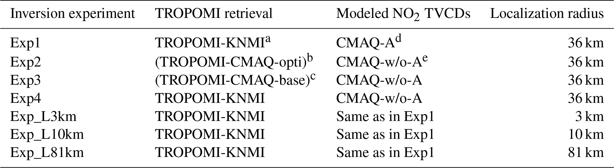
^a TROPOMI-KNMI refers to the standard TROPOMI retrieval product from KNMI. ^b TROPOMI-CMAQ-opti refers to the new TROPOMI NO₂ retrievals using the posterior CMAQ simulation from Exp1 as the a priori profile. ^c TROPOMI-CMAQ-base refers to the new TROPOMI NO₂ retrievals using the prior CMAQ simulation from Exp1 as the a priori profile. ^d CMAQ-A represents CMAQ NO₂ TVCDs calculated using satellite AKs. ^e CMAQ-w/o-A represents CMAQ NO₂ TVCDs calculated without applying satellite AKs.

2.5 Sensitivity experiments

We designed seven sensitivity inversion experiments to evaluate our inversion system (Table 1). The experiments Exp1–Exp4 were designed to analyze the impact of the a priori profile and AK on emission inversions. Exp_L3km, Exp_L10km, and Exp_L81km were designed to investigate the effect of different observation localization radius parameters on the emission inversion.

The retrieval of the tropospheric NO₂ TVCD is substantially influenced by the assumed a priori NO₂ profiles, which are used in the calculation of the air mass factor (AMF) that converts the slant column into the vertical column (Cooper et al., 2020; Huijnen et al., 2010; Douros et al., 2023). Due to the differences in the shape of the satellite and model a priori profiles, the satellite–model comparison is influenced by the shape of the a priori profile. There are two common ways to eliminate the impact of the a priori profiles on model–satellite comparisons: applying satellite averaging kernels to modeled partial columns or developing new satellite retrievals with modeled profiles instead of using the a priori profiles derived from the TM5-MP model (Douros et al., 2023; Eskes et al., 2022). The former method is the approach adopted in our study (i.e., Exp1 in Table 1), while the latter is used for sensitivity inversions (i.e., Exp2–Exp3 in Table 1). We used the posterior-emission-driven (derived from Exp1) CMAQ profiles in Exp2 and the prior-emission-driven CMAQ profiles in Exp3 to recalculate the satellite NO₂ TVCDs product. The set of new profiles have a horizontal resolution of 3 km over the D03 domain of the CMAQ model. The new TROPOMI NO₂ retrievals V_o, new for Exp2–Exp3 are derived from the new a priori profiles from CMAQ simulations as follows (Douros et al., 2023; Eskes et al., 2022):

$$\begin{array}{}\text{(7)}& {\displaystyle }{V}_{\mathrm{o},\mathrm{new}}={\displaystyle \frac{M^{\mathrm{trop}}}{M_{\mathrm{cmaq}}^{\mathrm{trop}}}}{V}_{\mathrm{o}},\text{(8)}& {\displaystyle }{M}^{\mathrm{trop}}\left(x_{\mathrm{m}}\right)={\displaystyle \frac{M^{\mathrm{trop}}\left(x_{\mathrm{a}}\right){\sum }_l{A}_l^{\mathrm{trop}}{x}_l^{\mathrm{m}}}{{\sum }_l{x}_l^{\mathrm{m}}}},\end{array}$$

where M^trop(x_m) is a new tropospheric air mass factor computed with the CMAQ model profile, M^trop(x_a) is the air mass factor depending on the TM5-MP model a priori profile, and V_o is the standard TROPOMI NO₂ retrieval. In Exp2 and Exp3, x_m represents the posterior-emission-driven CMAQ profiles and the prior-emission-driven CMAQ profiles, respectively. For Exp2 and Exp3, the modeled NO₂ TVCDs are calculated by directly integrating the partial NO₂ columns within the troposphere without applying satellite AK (CMAQ-w/o-A). Additionally, we include another experiment (Exp4) to compare the standard TROPOMI products with the model columns directly without applying AK. It should be noted that the comparison in Exp4 represents the influence from the a priori profile of TROPOMI retrievals.

2.6 Evaluation observations

The ground-based observations are used to evaluate the impact of the emission inversion constrained by the TROPOMI satellite retrievals on the improvement of the CMAQ simulations at the 3 km scale. The surface observations are obtained from the monitoring stations maintained by the China National Environmental Monitoring Center (CNEMC, http://www.cnemc.cn/, last access: 20 January 2024). Figure S1 shows the spatial location of the ground-based stations used to evaluate the CMAQ simulations. These stations are primarily located in densely populated areas of each city. NO₂ and O₃ measurements are used for inversion model evaluation in our study since NO₂ and O₃ concentrations are highly sensitive to the adjustment of NO_x emissions. The measurements of NO₂ concentrations are obtained via a chemiluminescence analyzer equipped with a molybdenum converter, which is known to be interfered with by other nitrogen oxides, such as peroxyacetyl nitrate (PAN) or nitric acid (HNO₃). As noted in Lamsal et al. (2008), NO₂ concentrations derived from observational instruments may be overestimated, and a correction factor (≤1) was proposed to address this bias. In this study, we do not apply corrections to the observations, and we discuss this point in Sect. 3.1.2. The systematic errors in ground-based NO₂ observations do not affect our conclusions; i.e., our posterior emissions have improved the CMAQ NO₂ simulation performance.

Figure 2 Comparison of the spatial distributions of TROPOMI NO₂ TVCD retrievals (the left column) with CMAQ-modeled NO₂ TVCDs driven by the prior (the second column) and posterior (the third column) emissions. The CMAQ-modeled NO₂ TVCDs are calculated using satellite averaging kernels. The last column is the scatterplot of the TROPOMI retrievals with the CMAQ-modeled NO₂ TVCDs simulated using the prior (blue) and posterior (red) emissions. From top to bottom, the rows represent winter (DJF), spring (MAM), summer (JJA), and autumn (SON).

3 Results

3.1 Evaluation of CMAQ simulations driven by posterior emissions

The CMAQ simulations driven by the proxy-based prior emission inventory are broadly consistent with the TROPOMI NO₂ TVCDs (Fig. S3) and surface-based NO₂ measurements (Fig. S4) at the 27 km grid scale but overestimate NO₂ concentrations at the 3 km scale over emission hotspot areas (Figs. 2 and 3). Zheng et al. (2021b) indicated that CTM simulations driven by proxy-based emission maps perform better at coarse resolutions of tens of kilometers since coarse grids generally contain entire administrative units and are less affected by emission spatial allocation based on proxies (e.g., population), which tend to misallocate the industrial emissions located in suburban areas to densely populated city centers. In this section, we evaluate the effectiveness of our inversion system by comparing the CMAQ simulations at the 3 km scale driven by the prior and posterior NO_x emissions, respectively, against TROPOMI NO₂ retrievals and the independent ground-based observations.

Figure 3 Comparison of the ground-based daily (a) NO₂ and (b) O₃ concentrations with the simulations utilizing prior and posterior NO_x emissions as the model input.

3.1.1 NO₂ tropospheric columns

The CMAQ simulations, driven by the posterior emissions, substantially narrowed the discrepancies between simulated NO₂ TVCDs and TROPOMI NO₂ retrievals (Fig. 2). In the simulations driven by prior emissions, the grid cells exhibiting a positive bias were more prevalent over the whole region, while the posterior simulations effectively correct this bias. Compared to the prior simulations, the RMSE differences between the posterior-simulated NO₂ concentrations and the observations were reduced by 58.32 %, 59.10 %, 69.73 %, and 70.03 %, respectively. Higher NO₂ TVCDs are typically observed over urban areas characterized by high population densities and extensive road networks. Using these factors (population densities and road networks) as spatial proxies in emissions mapping is thus justified to a certain degree. However, the NO₂ TVCDs from prior simulations indicate substantial overestimations in urban environments across various seasons, particularly in the central districts of Beijing, Tianjin, and Baoding, with the overestimation being the most pronounced in winter and autumn. This suggests that the prior emission inventory might have overestimated emissions in these areas. In contrast, the NO₂ TVCDs from posterior simulations show a considerable reduction in these overestimation errors when compared to the TROPOMI satellite observations, aligning more closely with the observed spatial gradient distribution patterns. Figure 4 illustrates the spatial maps of both prior and posterior NO_x emissions, highlighting the areas that contribute to the improvement observed in the simulated NO₂ concentration distributions.

Figure 4 The spatial map of the prior and posterior emissions for the four seasons in 2020. The last column shows the differences between the two emissions. From top to bottom, the rows represent winter (DJF), spring (MAM), summer (JJA), and autumn (SON).

The improvements in the simulated NO₂ TVCDs are more pronounced in spring and summer compared to autumn and winter. In the warmer months, due to NO₂'s short atmospheric lifetime, its concentrations are less influenced by long-range transport, leading to high-concentration regions being more localized around emission hotspots. The NO₂ TVCDs simulations in these seasons thus greatly benefit from our inversion-optimized emissions. In the cooler months, the prior simulations overestimate NO₂ TVCDs across most high-emission areas, and the posterior simulations can also mitigate these overestimations. Despite these improvements, the posterior simulations still show overestimation errors in the southern region of our study area during the colder seasons. This might be attributed to the longer NO₂ lifetime in colder conditions, which increases its susceptibility to regional transport and accumulation. Specifically, pollution transport from sources south of Baoding contributes to the overestimated NO₂ levels in this region. Our inversions at the 3 km scale were limited to optimizing emissions in the innermost domain and did not address emissions outside this area. Expanding the simulation domain could potentially rectify the persisting overestimation errors near Baoding, although this would require additional computation resources.

3.1.2 Surface NO₂ and O₃ concentrations

As shown in Fig. 3, the daily NO₂ concentrations modeled with input from the bottom-up inventory are substantially overestimated, while simulations utilizing posterior NO_x emissions have considerably improved the accuracy of the surface NO₂ simulations. Over the entire year of 2020, the RMSE between the modeled and observed NO₂ concentrations decreased from 38.93 µg m⁻³ in the prior-emission-based simulations to 13.48 µg m⁻³ in the posterior simulations. However, it is important to note that while the posterior simulations closely matched observed concentrations, the improvement in NO₂ simulations during summer was relatively limited. One possible reason for the large simulation biases in summer is the lack of satellite observation constraints during the rainy season (Fig. S2a). Additionally, the AK describes the sensitivity of the satellite instrument to tracer concentrations at different altitudes, and the sensitivity is small near the surface (Eskes and Boersma, 2003). This suggests that satellite retrievals of NO₂ columns offer weak constraints on ground emissions, especially in summer, as indicated by smaller AK values near the surface compared to winter (Fig. S5), thereby resulting in limited improvements in NO₂ simulations. It is worth mentioning that measurements of NO₂ concentrations via the molybdenum converter may be overestimated due to interference from other reactive oxidized nitrogen species. Lamsal et al. (2008) proposed a correction factor of less than 1 for NO₂ observation data. In this study, NO₂ observations are lower than prior simulations; therefore, applying such corrections to the NO₂ observations would not affect the conclusions of our study.

Furthermore, we have classified the observation stations into two categories based on NO₂ concentration characteristics, population density, and emission patterns: low-pollution areas and high-pollution areas. The low-pollution areas refer to the two northern cities in the D03 domain, Zhangjiakou and Chengde, where NO₂ concentrations are relatively low. The observation stations in all other urban areas are classified as high-pollution stations. Figure S6 presents a comparison between CMAQ simulations and ground-based observations in different pollution regions. Compared to other highly polluted urban areas, the posterior NO₂ simulations in Zhangjiakou and Chengde show much better consistency with observations during summer. This indicates that in regions with low surface emissions, the accuracy of posterior simulations in summer is relatively high. Furthermore, it reinforces the finding that in highly polluted urban areas, the constraint of satellite NO₂ column measurements on surface emissions in summer is weaker, leading to an overestimation in posterior simulations.

In terms of O₃ concentrations, the optimized NO_x emissions also improve the simulation accuracy since NO_x can influence the formation and depletion of O₃. The RMSE between the simulated O₃ concentrations and ground-based O₃ observations decreased from 26.11 to 13.91 µg m⁻³. The overestimation of the bottom-up NO_x emissions leads to negative biases in the O₃ simulations throughout the year. However, during summer, the deviations between simulated O₃ concentrations and observations are less pronounced compared to those observed in NO₂ simulations. This is because the simulation of NO₂ is significantly influenced by surface NO_x emissions. In contrast, simulated O₃ concentrations are affected by multiple factors, with NO_x emissions being only one of them. For instance, during summer, increased biogenic emissions and enhanced photochemical activity play critical roles. As a result, even in the prior O₃ simulations, the discrepancies between modeled and observed O₃ values are less pronounced compared to those in NO₂ simulations. Although the posterior O₃ simulations align well with observations, they remain slightly below the observed values, indicating that the posterior NO_x emissions may still be overestimated during summer.

3.2 Spatial-temporal variations in the posterior NO_x emissions

3.2.1 Spatial distribution of the NO_x emissions

The posterior emissions have led to substantial improvements in the accuracy of the 3 km CMAQ simulations, which could be attributed to the improved NO_x emission distribution patterns after being constrained by satellite observations. Here, we first analyze the changes in the spatial distribution of posterior NO_x emissions at the 3 km scale.

Figure 4 shows the spatial map of the prior and posterior emissions for the four seasons in 2020. The prior emission maps show the highest intensity in urban centers, including Beijing, Baoding, and Tianjin urban areas. The satellite-constrained posterior emissions maintain a similar spatial distribution with the emission hotspots broadly consistent with the prior emission inventory. However, the comparison between posterior and prior emissions (third column of Figs. 4 and S7) reveals that the posterior emission maps substantially reduce emissions in urban centers and redistribute these emissions to other regions. For instance, emissions from inter-city transportation (see the third column of Fig. S7 with the overlay of the road map) are notably increased, particularly during spring and summer. As seen in the spatial map of the total population, as shown in Fig. S8, the grids with decreased emissions in the posterior emission maps are consistent with areas of high population density, especially in summer. The areas with high population density are mainly located in the city center. This indicates that at the kilometer-scale spatial resolution, emission inventories allocated based on the population density as a spatial proxy tend to overestimate emissions in grid cells located in urban centers in Beijing and its surrounding areas.

The posterior NO_x emissions for the year 2020 (657 kt NO_x) decreased by 23.7 % compared to the prior inventory (861 kt NO_x) (Fig. S7). The largest reduction in emissions occurs in winter and autumn, with a decline of 44.5 % and 36.4 %, respectively. The total emissions during summer are comparable to the prior emission inventory. This is mainly due to the weaker reduction in emissions occurring in urban areas when compared to other seasons coupled with a more pronounced increase in emissions in non-urban areas, such as the road network, which leads to regional total emissions remaining at relatively high levels. The bottom-up prior inventory is based on actual activity level data and emission factors, which can somewhat reflect the emission reductions during the COVID-19 lockdown period. However, due to statistical errors and the misrepresentation of emission factors, the prior emission inventory still fails to provide an accurate estimate of the regional total NO_x emissions.

Figure 5 Time series of the bottom-up and top-down daily NO_x emissions for domain D03 and Beijing. The dashed gray line indicates the Chinese Lunar New Year, which also marks the date when Beijing began implementing COVID-19 control measures. The dashed blue line represents the start date of control measures following the sudden outbreak at the Xinfadi market in Beijing. The gray shaded area represents the period affected by COVID-19 measures in 2020, and the light blue shaded area highlights the time frame impacted by the Xinfadi market outbreak.

3.2.2 Temporal variations in the NO_x emissions

Performing emission inversion on a daily basis can illustrate daily emission changes, which are difficult to capture in the prior emission inventory. The posterior emissions reflect the reduction and recovery in emissions in early 2020 (Fig. 5) driven by the implementation and relaxation of COVID-19 containment measures as well as the impact of the Chinese Lunar New Year holiday. The reduction in NO_x emissions due to the pandemic lockdown measures lasted from early 2020 to mid-March 2020, with emission levels gradually returning to normal by late April. However, although the prior emission inventory partially reflects real monthly production activity levels, it fails to accurately capture such dynamic changes in emissions. The prior emission inventory only distinctly captures the emission reduction that occurred from early February to mid-February 2020 and was mainly caused by the Chinese Lunar New Year. In addition, the posterior emission estimates also indicate a period of emission reduction and rebound from mid-June to mid-July 2020, coinciding with the sudden outbreak of the epidemic and the subsequent lockdown measures implemented at the Xinfadi market in Beijing, China.

The satellite observations introduce considerable seasonal variations in the posterior NO_x emissions, while the prior NO_x emission inventory does not exhibit obvious seasonal variations. In winter, emissions are overestimated, mainly due to the overestimation of urban emissions (Fig. 4). In summer, total emissions are comparable to the posterior emissions because the emission reduction in densely populated urban centers is compensated for by an increase in emissions from other regions. The seasonal variation in the posterior NO_x emission estimate in our research is similar to the results obtained by previous studies (Wang et al., 2007; Qu et al., 2017; Miyazaki et al., 2017). Qu et al. (2017) utilized OMI measurements to infer the NO_x emissions in China, and the seasonal pattern of NO_x emissions for China and Beijing is consistent with our study. These studies, along with the results of our study, indicate that while the prior emissions tend to have the lowest levels in summer, the posterior emissions are higher in summer, when they are comparable to or even higher than winter emissions. Since we focus only on anthropogenic emissions in urban areas, this study does not include natural emissions from soil and lightning sources, except for the biogenic emissions, which are dynamically generated by the MEGAN model. However, these natural sources are implicitly included in the posterior emissions. Previous studies have attributed the summer peak of NO_x emissions to contributions from natural sources since high temperatures in summer lead to more emissions from soil and fertilization, and there is also a higher frequency of lightning (Miyazaki and Eskes, 2013; Qu et al., 2017). We select grids where anthropogenic and biogenic sources account for more than 90 % of the total emissions, respectively. The seasonal variations (Fig. 6) show that the grids dominated by biogenic sources contribute emissions mainly during the warm seasons, when higher temperatures enhance the release of NO_x from both soil and fertilized fields.

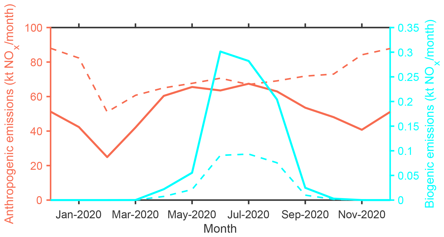
Figure 6 Monthly NO_x emissions from the grids dominated by anthropogenic (red) and biogenic (cyan) sources. The solid and dashed curves represent the posterior and the prior NO_x emissions, respectively.

4 Discussions

4.1 Impact of the a priori profile and averaging kernel on the emission inversion

Four experiments are designed to test the impacts of the a priori profile and satellite AK on the NO_x emission inversions, and the settings are described in Sect. 2.6 and Table 1. The daily posterior emission time series from the four sets of experiments are shown in Fig. 7. The results indicate that the emissions obtained from the four sets of experiments are generally consistent and robust throughout the year except for summer. First, the differences between Exp1, Exp2, and Exp3 are relatively small, indicating that the impacts of the two optimal satellite–model comparison methods on the inversions are nearly equivalent. In contrast, the emissions obtained from Exp4 are slightly lower than those from Exp1 during summer.

Due to the weaker AK sensitivity at altitudes below 2 km during summer (Fig. S5), Exp1, which uses AK in the model NO₂ column calculation, yields lower model columns in summer compared to Exp4. As a result, the positive bias in model columns with satellite columns is smaller in Exp1, leading to higher emissions compared to Exp4. In winter, AK values are relatively higher than in summer and increase rapidly with altitude within 2 km. Consequently, the AK-based model columns are better at reflecting emissions in the lower atmosphere in winter than in summer. Both Exp2 and Exp3 use model-derived vertical column concentrations without using AK, which is similar to Exp4, but the emission inversion results are higher than Exp4 in summer. This is because although the model vertical columns are calculated using the same method as for Exp4 in summer, the new satellite products calculated using CMAQ-based a priori profiles show higher columns during summer compared to the standard satellite product, especially in emission hotspots (Fig. 8). Therefore, the posterior emissions are higher than those of Exp4 in summer. Douros et al. (2023) also produced a new TROPOMI product over Europe using the modeled profiles from the high-resolution regional model (0.1° × 0.1°), and they also found an increase in the tropospheric columns at emission hotspots over the summer months.

Figure 7 The daily posterior emission time series from the sensitivity experiments Exp1–Exp4 in the domain D03.

The comparison between Exp2 and Exp3 shows similar emission inversion results. This is because the two new satellite products are consistent in their values (Fig. S9), which are calculated based on the CMAQ profiles simulated by the prior and posterior emissions, respectively. This indicates that the vertical profile shapes of the modeled NO₂ concentrations driven by both prior and posterior emission inventories are similar, provided that the model and model resolution settings are consistent. Therefore, when utilizing newly generated satellite products for assimilation and inversion, it may not be necessary to update the a priori profiles in each assimilation step, and the model profiles simulated using the prior emissions can be used to calculate new satellite products before the inversion process. This result is similar to the study by Cooper et al. (2020), which performed experiments using synthetic observations to test the a priori profile on the emission inversions. Their study found that the inversion error is the lowest when the a priori profiles are updated during the assimilation process, but using the profile from the initial model state without updating during the assimilation can also get accurate inversions because their profile shapes are similar regardless of whether they are updated. Since the region D03 in our study is a high-emission area, its profile shape is mainly dominated by surface emissions. For regions with lower anthropogenic emissions, the free troposphere's contribution to the satellite-observed column is likely more pronounced. This enhanced contribution increases the profile shape's sensitivity to surface emission changes, which may result in significantly different inversion results compared to high-emission regions.

Figure 8 Comparison of the spatial distribution of the NO₂ TVCDs from the new TROPOMI NO₂ retrieval products and the standard TROPOMI-KNMI product in summer. TROPOMI-CMAQ-opti refers to the new TROPOMI product using the posterior CMAQ simulation as the a priori profiles. TROPOMI-CMAQ-base refers to the new TROPOMI product using the prior CMAQ simulation as the a priori profiles.

Figure 9 Scatterplots of the TROPOMI NO₂ TVCDs and the CMAQ simulated NO₂ TVCDs from the inversion experiments with a localization parameter of 3, 10, 36, and 81 km, respectively. (a) December 2019. (b) June 2020.

4.2 Impact of the observation localization parameters on the emission inversion

The observation localization of LETKF is implemented by assimilating observations within a specified local area and using a decay function to reduce the impact of observations as the distance from the analysis grid increases. To evaluate the impact of different L values on the NO_x emission inversions, we perform three additional experiments with L= 3 km (Exp_L3km), L=10 km (Exp_L10km), and L=81 km (Exp_L81km), respectively. The experiments were conducted for the periods of December 2019 and June 2020, and then the posterior NO₂ simulations were evaluated through comparisons with TROPOMI NO₂ TVCDs (Fig. 9).

The results showed that the three additional sensitivity experiments with L values of 3, 10, and 81 km were all able to optimize NO_x emissions to some extent. However, Exp_L36km still performed the best overall. In winter, the effectiveness was the weakest for Exp_L81km followed by Exp_L3km. The inversion results from Exp_L10km were closely comparable to those of Exp_L36km, though the statistical metrics were slightly lower than those of Exp_L36km. In summer, while the statistical metrics of Exp_L10km were slightly weaker than those of Exp_L81km, the posterior simulations in high-value regions showed better consistency with observations compared to Exp_L3km and Exp_L81km. Exp_L81km exhibited greater dispersion relative to observations, possibly because the 81 km ×81 km area included a large number of observations, which could interfere with the optimization of emissions in the target grid. On the other hand, observations at longer distances were already outside the influence range of emission sources from the target grid. The 3 km radius area contains too few observations and has insufficient responsiveness to the transport of emissions from the target grid. Testing the 10 km localization parameter is meaningful: if the optimization results with L=10 km surpass those with L=36 km, it would suggest that fewer observations need to be assimilated, thereby reducing computational resource consumption. This is because the LETKF assimilation algorithm employs explicit localization, meaning that only observations within the localization radius centered on each grid cell are assimilated.

Since Exp_L36km yielded the best results in this study, using a 36 km localization radius is reasonable. In practice, the selection of an appropriate localization parameter may require extensive tuning or adaptive adjustments based on meteorological conditions, but this will impose huge computational burdens. Therefore, we tend to choose a theoretically reasonable parameter or observation localization.

4.3 Future improvement directions

The uncertainties in the NO_x emission inversion in this study arise from multiple sources, including inaccurate depictions of the chemical and physical mechanisms in the CTMs, methodological challenges in matching model simulations to satellite column concentrations, errors inherent to satellite retrievals, and limitations of current assimilation techniques, among others. The lifetime of NO₂ in the atmosphere is a key factor to relate satellite-observed concentrations to emissions, and errors in this could introduce a seasonally dependent bias.

In terms of our emission inversion framework, several factors can introduce uncertainties to the inversions. Firstly, the settings of the CTM simulations, such as the configuration of the model layers, might be important for the depiction of the column concentrations where future improvements can be made. Secondly, the TROPOMI satellite's local overpass time in the mid-afternoon means that the inversion system still cannot capture hourly variations in NO_x emissions, and therefore the hourly allocations in the posterior emissions are the same as in the bottom-up inventory. Besides, the weak sensitivity of the satellite measurements to the NO₂ concentrations at lower altitudes leads to limited constraints on surface emissions, particularly during summer (Miyazaki and Eskes, 2013). A recent study by He et al. (2022) suggests that the incorporation of hourly ground-based observations may help to improve surface emission inversions. The Geostationary Environment Monitoring Spectrometer (GEMS), launched in 2020, monitors atmospheric pollutants over Asia from a geostationary orbit, providing hourly observation data. Future work will involve assimilating GEMS satellite data, which will not only help track daily emission changes but also reveal the hourly variation patterns of emissions. In addition, although data assimilation methods take into account the influence of the observations outside of the target grid, the optimal influence distance is difficult to determine. An improved observation assimilation scheme, such as taking into account the correlation between the emissions in the target grid with the observations within the localization area may hold promise for improving the accuracy of emissions inversions. In our model assimilation system, using unoptimized emissions from D01 and D02 to simulate boundary conditions might introduce uncertainties in the emission inversion near the D03 boundaries. These uncertainties are more pronounced in winter due to the longer NO₂ lifetime and stronger atmospheric transport effects. As shown in Fig. 2, simulated concentrations near the southern boundary of D03 in autumn and winter are higher than observations, likely due to the influence of unadjusted D02 boundary conditions, which may lead to underestimated emission inversion results in these regions. In contrast, the impact of D02 boundary conditions on D03 is weaker in spring and summer. If computational resources are sufficient, we recommend optimizing emissions in D02 to reduce the influence of boundary conditions on D03. Alternatively, we could consider expanding the D03 domain by extending its boundaries outward by approximately 100 km (the distance potentially influenced by boundary conditions). After completing the assimilation experiments for D03, the extended area could be trimmed, retaining only the central region that is minimally affected by boundary conditions for NO_x emission analysis.

Finally, our study lacks independent validation of the vertical NO₂ profile simulations to assess the relative contribution of free tropospheric activity to satellite-observed column concentrations under varying emission scenarios and to analyze the sensitivity of profile shapes to surface emission changes. Future work will incorporate observational validation and inter-model comparisons to address these limitations.

5 Conclusions

The advantages of TROPOMI's small footprint and near-daily global coverage enable research on fine-scale emission inversions. In this study, we develop an advanced emission inversion system by combining the CMAQ nested model with the LETKF algorithm to assimilate TROPOMI NO₂ retrievals. We obtain the posterior NO_x emission maps on a daily basis at 3 km scales in Beijing and surrounding areas. The posterior emissions offer a more reasonable spatial disaggregation and capture temporal changes effectively. In terms of spatial distribution, we further explain how proxy-based spatial allocation schemes in the prior emission inventory tend to overestimate urban emissions. In terms of temporal variations, the posterior emissions show considerable seasonal changes and provide timely insights into daily emission variations, such as the emission reductions induced by COVID-19 control measures. We conduct sensitivity experiments to analyze the impact of the a priori profiles used in the satellite retrievals and the use of AKs for calculating model NO₂ columns on the inversion results. The experiments indicate the robustness of our inversion, with a greater sensitivity to different model–satellite comparison schemes in summer. Our posterior NO_x emissions improve the accuracy of the CMAQ simulations of NO₂ and O₃ concentrations at 3 km scales for the whole year in 2020. However, in summer, despite notable improvements in the CMAQ simulations, a positive model bias persists, implying that TROPOMI NO₂ column retrievals provide weaker constraints on surface NO_x emissions in summer. Overall, the high-resolution NO_x emission inversion framework developed in this study improves our understanding of the spatial distribution patterns and the daily variations in anthropogenic NO_x emissions at fine scales, providing an instructive example for improving fine-scale modeling and prediction.