High-resolution mapping of on-road vehicle emissions with real-time traffic datasets based on big data

On-road vehicle emissions play a crucial role in affecting fine-scale air quality and exposure equity in traffic-dense urban areas. They vary largely on both spatial and temporal scales due to the complex distribution patterns of vehicle types and traffic conditions. With the deployment of traffic cameras and big data approaches, we established a bottom-up model that employed interpolation to obtain a spatially continuous on-road vehicle emission mapping for the main urban area of Jinan, revealing fine-scale gradients and emission hotspots intuitively. The results show that the hourly average emissions of nitrogen oxides, carbon monoxide, hydrocarbons, and fine particulate matters from on-road vehicles in urban Jinan were 345.2, 789.7, 69.5, and 5.4 kg, respectively. The emission intensity varied largely with a factor of up to 3 within 1 km on the same road segment. The unique patterns of road vehicle emissions within the urban area were further examined through time series clustering and hotspot analysis. When spatial hotspots coincided with peak hours, emissions were significantly enhanced, making them key targets for traffic pollution control. Based on the established emission model, we predicted that the benefits of vehicle electrification in reducing vehicle emissions could reach 40 %–80 %. Overall, this work provides new methods for developing a high-resolution vehicle emission inventory in urban areas and offers detailed and accurate emission data and fine spatiotemporal variation patterns in urban Jinan, which are of great importance for air pollution control, traffic management, policy-making, and public awareness enhancement.

1 Introduction

The rapid increase in the number of vehicles in recent years has brought convenience to people's travel and daily lives. At the same time, it has also posed considerable challenges, including traffic congestion, severe air pollution, and adverse health impacts (Uherek et al., 2010; Guo et al., 2014; Zhang et al., 2018; Shi et al., 2023). In urban areas with dense populations in particular, vehicle emission acts as a major cause of air quality deterioration, which has attracted widespread public attention (Ramacher et al., 2020; Qi et al., 2023). To evaluate the environmental impacts of this, researchers and stakeholders have established on-road vehicle emission inventories to estimate the amount of air pollutants emitted from vehicle exhausts into the atmosphere (Zhang et al., 2018). Considering vehicle population growth, stringent emission standards, the phasing out of old vehicles, and vehicle electrification, the spatiotemporal emission characteristics of vehicles in the new period may have changed (Wen et al., 2023; Zhu et al., 2023). Therefore, developing up-to-date dynamic on-road vehicle emission inventories that align with current urban traffic flow conditions is urgently needed and is quite important for vehicle pollution control and urban air quality improvement.

Emission factors, defined as the number (or mass) of pollutants emitted per unit of activity, are one of the basic data types used for the development of emission inventories. Several methods for determining on-road vehicle emission factors have been used in real-world conditions, such as street canyon and road tunnel studies (Brimblecombe et al., 2015; Zhang et al., 2015), remote sensing (Davison et al., 2020), and onboard measurements (Jaikumar et al., 2017). Other methods involve the estimation of air dispersion by tracking a trace gas that can be added or emitted by traffic (Belalcazar et al., 2010) and the use of the eddy-covariance (EC) technique to quantify emissions based on atmospheric turbulence (Conte and Contini, 2019). Although previous measurements have yielded convincing emission factors for local vehicles, some limitations in the development of emission inventories have not yet been adequately addressed. Road traffic sources, belonging to mobile sources, are characterized by low emission heights, densely populated emission areas, and obvious spatiotemporal heterogeneity (Liu et al., 2018; Ding et al., 2023). The traffic flows, vehicle compositions, and vehicle speeds vary dramatically over short periods and distances, affecting the emission characteristics of traffic sources (Chen et al., 2020; Jiang et al., 2021). As a result, the accuracy of vehicle emission inventories largely depends on the quality of the input data on traffic conditions (Ding et al., 2021; Romero et al., 2020). Conventional vehicle emission inventories are usually established by using a top-down approach, based on statistical data, including vehicle population, mileage, and fuel types (Cai and Xie, 2007; Fameli and Assimakopoulos, 2015). These inventories are generally temporally static and spatially rough, lacking high-spatiotemporal-resolution data to characterize road vehicle emission. In the past dozen years, several advanced technologies, such as GPS-equipped floating cars, open-access congestion maps, and intelligent transportation systems (ITSs), have been applied to develop high-resolution traffic emission inventories (He et al., 2016; Zhang et al., 2018; Liu et al., 2018; Maes et al., 2019; Ghaffarpasand et al., 2020). Exploiting taxi GPS data can infer the spatial and temporal variation patterns of urban traffic emissions, with the heaviest traffic volumes and emission hotspots often discovered in city centers (Luo et al., 2017; Liu et al., 2019). Open congestion maps provide real-time traffic information, making traffic volume inference timely. A more detailed vehicle emission inventory in Beijing was developed based on open congestion maps, indicating significant impacts on vehicle emissions caused by traffic restrictions (Yang et al., 2019). In addition, several studies have substantially improved vehicle emission inventories by collecting detailed, high-precision, and real-time monitoring data with ITSs. For example, the spatial resolution of an hourly emission inventory in Xiaoshan District in Hangzhou was increased by 1–3 orders of magnitude through an ITS (Jiang et al., 2021). In the study of Jiang et al. (2021), emission hotspots exhibited sharp small-scale variability and strengthened during peak hours. By means of an ITS, the spatiotemporal dynamics of vehicle emissions in Guangdong Province were also revealed (Ding et al., 2023). It was found that gasoline passenger cars were the main contributors to carbon monoxide (CO) and hydrocarbon (HC) emissions during peak hours, while diesel trucks were the dominant source of emissions of nitrogen oxides (NO_x) and fine particulate matters (PM_2.5) at night. Despite the above improvements, previous inventory compilation techniques for on-road vehicles have some limitations due to incomplete traffic data, insufficient vehicle details, or high costs of wide coverage. More comprehensive data need to be obtained using cost-effective methods to achieve long-term and wide-area coverage, particularly in less developed cities.

Recently, traffic camera networks have been widely adopted and are readily available, providing extensive coverage in critical urban areas. They have the capability to continuously capture nearly all vehicles driving on roads (Liu et al., 2024), thus providing an opportunity to develop an ultra-fine-resolution vehicle emission inventory. To some extent, large-scale real-time traffic datasets are crucial for elucidating the spatiotemporal variations in on-road vehicle emissions (Wu et al., 2022). However, the main concern is that processing and analyzing a large amount of data are challenging and time-consuming tasks (Lv et al., 2023). Compared to traditional statistical methods, big data approaches offer apparent advantages in handling, validating, analyzing, mining, and visualizing large-scale, multi-source, and structurally complex monitoring data. At present, big data have been used for air pollution mapping with much higher spatial precision than fixed-site monitoring (Apte et al., 2017). In addition, Deng et al. (2020) used a big data approach to establish a high-resolution and large-region vehicle emission inventory in the Beijing–Tianjin–Hebei region, but the inventory is only for trucks. With the application of big data techniques, it becomes feasible to develop accurate, practical, and dynamically updatable urban traffic emission inventories with high spatiotemporal resolution.

Note that even widely distributed traffic cameras are unlikely to achieve spatially continuous observations. The spatial gaps of meters to kilometers between fixed traffic cameras determine the upper resolution limit of the bottom-up on-road vehicle emission inventory. Therefore, alternative approaches are needed to complement the observation data and fill the gaps. Interpolation, a useful data processing method, can preserve the emission data at the original monitoring points while maximizing the reproduction of the spatial gradient of emissions over short distances (10 m–1 km). Jeong et al. (2019) innovatively applied spatial interpolation models to achieve a more accurate estimation of methane emission from a landfill. Similarly, exploiting spatial interpolation to the estimation of vehicle emissions can compensate for spatial gaps between traffic monitoring points, making on-road vehicle emission mapping dynamic and continuous. Due to the drastic change in air pollutant concentrations over short distances in urban areas caused by the uneven spatial distribution of traffic sources (Apte and Manchanda, 2024), refined vehicle emissions through interpolation will of course provide an effective reference for the improvement and interpretation of air pollution mapping.

As the capital of Shandong Province and an important transportation hub in northern China, Jinan is confronting severe air pollution. The number of vehicles in Jinan exceeded 3 million in 2020, and vehicular emissions are a significant source of urban air pollutants. Jinan has basically achieved full coverage of traffic camera monitoring, which allows us to obtain traffic data for each road segment. In this study, we combined traffic camera recordings with field surveys, making the framework applicable to most cities. By using a bottom-up approach to calculate emissions and pioneering the application of spatial interpolation, we successfully established a high-resolution (temporal resolution of 1 h and spatial resolution of 50 m×50 m) on-road vehicle emission mapping. With the high-efficiency processing capabilities of big data approaches and the accumulation of hourly data for nearly 1 year, the seasonal variations, weekday and weekend differences, diurnal changes, and spatial distribution patterns of vehicle emissions for multiple pollutants were analyzed and revealed. Through time series clustering and hotspot analysis, the different diurnal variation patterns and hotspot areas of vehicle emissions on urban roads were further identified. Additionally, considering the rapid development of new energy vehicles (NEVs), future scenarios were designed to predict the positive impact of vehicle electrification on on-road traffic emissions. Finally, the validation of the developed on-road vehicle emission inventory was conducted by comparing with other inventories.

2 Methodology and data

2.1 Road network and real-time traffic monitoring

Jinan is located in the middle of the Beijing–Tianjin–Hebei region and the Yangtze River Delta region, serving as an important urban transportation hub in northern China. As of 2023, it had a population of over 9.43 million, with a GDP of CNY 1276 billion. The total length of the road network was around 18 356 km within a geographical area of 10 244 km². There were 3.39 million private vehicles (motorcycles excluded) in Jinan, with an average annual growth rate of 7 % since 2019. However, the construction of roads and rail transit has lagged behind. Limited traffic space was incompatible with the rapidly increasing number of vehicles, leading to frequent traffic congestion, especially in urban areas. In addition, driving restrictions for trucks in peak hours were implemented in the main urban area by the local government. In this study, the main urban area of Jinan (within the inner-ring expressway) was selected to collect real-time traffic data from monitoring points and further calculate the on-road vehicle emissions (see Fig. 1). There were a total of 1189 traffic monitoring points in the main urban area, which used fast cameras to capture all vehicles passing by, identify the vehicle categories, and record the traffic flows. Four categories of vehicles were recognized automatically, including light-duty vehicles (LDVs), heavy-duty vehicles (HDVs), new energy light-duty vehicles (NELDVs), and new energy heavy-duty vehicles (NEHDVs). All the roads in the main urban area were classed as highways, expressways, arterial roads, or minor arterial roads and were divided into numerous segments by traffic monitoring points. The gaps between two monitoring points ranged from 10 m to 3 km. The hourly data of vehicle flows and categories were obtained with image processing, object detection, and image recognition algorithms.

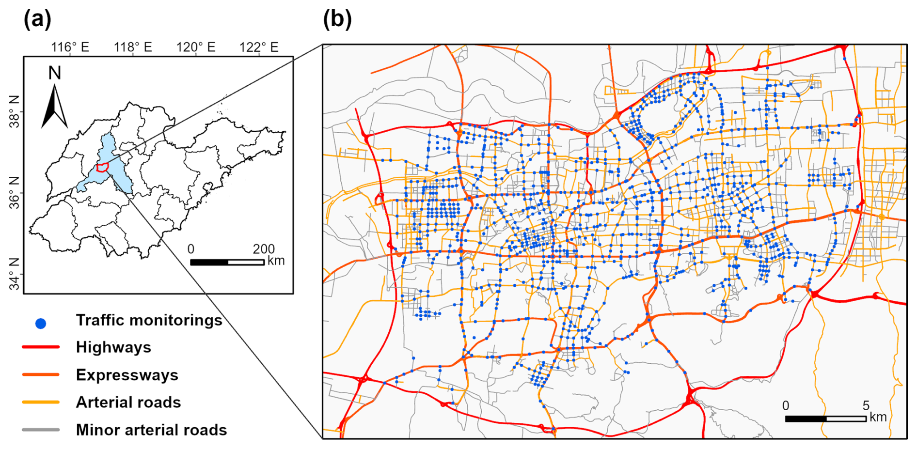
Figure 1 Road network and the real-time traffic monitoring points in the main urban area of Jinan. (a) Map shows Jinan (the blue area) located in Shandong Province, China, with the main urban area within the red borders. (b) Real-time traffic monitoring achieved full coverage over the main urban area of Jinan.

2.2 Data collection and processing based on big data approaches

Big data methods were employed in this study to calculate the high-resolution emissions of air pollutants. The accuracy largely depended on the quality of input data of traffic and meteorological conditions (Romero et al., 2020). To obtain real-time traffic information, the hourly flow data for the four categories of vehicles measured at each monitoring point were collected from 1 April 2023–29 February 2024. The fractions of specific vehicle types were determined based on our previous surveys conducted on typical roads within urban areas of Jinan in April 2022 (Wang et al., 2025), and the classification method is introduced in Sect. 2.3. The hourly meteorological data during the study period at the surface level were adopted from ERA5 (https://cds.climate.copernicus.eu, last access: 29 March 2024) with a horizontal resolution of 0.25° (Hersbach, et al., 2023). They were integrated with the traffic dataset with higher resolution by a “snapping” procedure on the basis of the nearest geographical coordinates. Meteorological data were used for environmental corrections of emission factors. In this process, we determined the local temperature and humidity ranges rather than the exact values and assigned specific correction coefficients accordingly.

With the hourly traffic and meteorological data, the on-road vehicle emissions of primary pollutants, including NO_x, CO, HC, and PM_2.5, were calculated and visualized. Figure 2 shows the framework of data processing for vehicle emission calculation and mapping. Specifically, the original datasets of traffic monitoring with approximately 106 million records were collected and integrated with meteorological data for subsequent data storage and management. Then, the data underwent extensive pre-processing, including cleaning, integration, transformation, and reduction. After that, the original data were consolidated into a structured dataset comprising 5.5 million sets of records. Each record set included multiple parameters of traffic flows for different vehicle types, emission correction factors (depending on meteorological conditions and vehicle speed), road information, and timestamps. The record sets were further used to calculate vehicular emissions and analyze their spatiotemporal distribution characteristics, ultimately aiding in understanding the status of urban vehicle emissions and formulating corresponding control strategies.

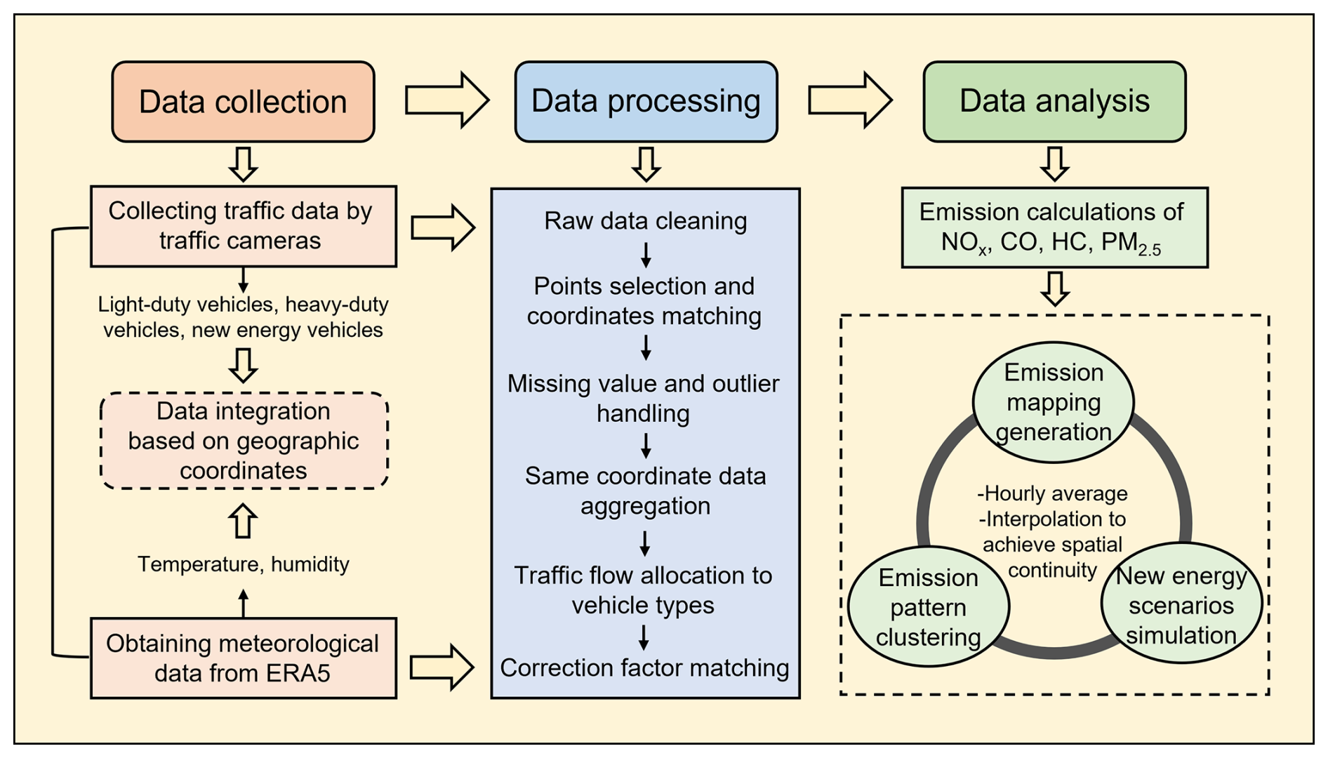
Figure 2 Model framework for high-resolution mapping of on-road vehicle emissions based on big data approaches.

2.3 Vehicle emission calculations and hyperfine-resolution mapping

The hourly emissions of air pollutants, including NO_x, CO, HC, and PM_2.5, at each road segment were calculated based on traffic flows, vehicle speeds, vehicle categories, road segment length, and emission factors (see Eq. 1) (Zhang et al., 2016; Yang et al., 2019; Jiang et al., 2021). Considering emission variations caused by local conditions, localized correction coefficients were adopted in this study for adjustment in emission factors (see Eq. 2):

$$\begin{array}{}\text{(1)}& E_{h,l,j}={\sum }_t{\text{EF}}_{c,j}\times T{F}_{c,h,l}\times L_l,\end{array}$$

where $E_{h,j,l}$ is the total emissions of pollutant j on road link l at hour h, in units of grams per hour (g h⁻¹). EF_c,j is the localized emission factor of pollutant j for vehicle category c, in units of grams per kilometer (g km⁻¹). ${\text{TF}}_{c,h,j}$ is the traffic flow of vehicle category c on road link l at hour h, in units of vehicles per hour (vehicles h⁻¹). L_l is the length of road link l, in units of kilometers (km).

$$\begin{array}{}\text{(2)}& {\text{EF}}_{c,j}={\text{BEF}}_{c,j}\times \mathit{\phi }\times \mathit{\gamma }\times \mathit{\lambda }\times \mathit{\theta }\end{array}$$

Here, BEF_c,j is the comprehensive baseline emission factor of pollutant j for vehicle category c, in units of grams per kilometer (g km⁻¹), and φ, γ, λ, and θ are the dimensionless environmental correction coefficient, traffic condition correction coefficient, deterioration correction coefficient, and vehicle usage condition correction coefficient (e.g., the load of diesel vehicles), respectively. All comprehensive baseline emission factors and correction coefficients were adopted from the Technical Guide for the Compilation of Atmospheric Pollutants Emission Inventory from Road Motor Vehicles (Trial) (MEE, 2014).

To achieve accurate emission calculations, the traffic flows for fuel light- and heavy-duty vehicles were allocated to eight specific types of vehicles, including light-duty passenger vehicles (LDPVs), middle-duty passenger vehicles (MDPVs), heavy-duty passenger vehicles (HDPVs), light-duty trucks (LDTs), middle-duty trucks (MDTs), heavy-duty trucks (HDTs), public buses, and taxis. This classification followed the national standard (GA802-2019) (see Table S1 in the Supplement). The distribution coefficients for the eight types of vehicles were based on the hourly vehicle proportions from field surveys on different roads in urban Jinan, as reported in our previous study (see Table S2 in the Supplement) (Wang et al., 2025). In addition, environmental correction was conducted mainly based on temperature and humidity, which varied largely from season to season, as detailed in Tables S3–S6 in the Supplement. Regarding the traffic condition correction, coefficients were determined based on the average vehicle speed intervals (see Tables S7–S8 in the Supplement). Different types of road segments, as well as the same type of road segments during peak and off-peak hours, were assigned with differential vehicle speed intervals based on real-time road conditions from Gaode Maps (see Table S9 in the Supplement). Note that new energy vehicles were deemed zero emission in this study, and the evaporative emissions of HC were excluded due to the complex sensitivities to fuel properties and environmental conditions (Jiang et al., 2021).

To present spatially continuous vehicle emission maps, spatial interpolation of hourly average emission intensities was conducted to fill in the gaps between discrete monitoring points. Compared to directly filling in the entire road segment with a single value, spatial interpolation allowed for the determination of pollutant emission rates at any point along the road, thereby generating emission maps that were more representative of real-world conditions. Nearest neighbor interpolation was uniformly selected for all four air pollutants due to its maximal preservation of the original emission data at the monitoring points. For a given point with unknown data, nearest neighbor interpolation does not create a new value but instead replicates the value of the known point located at the shortest distance (Olivier and Hanqiang, 2012). The proposed method demonstrated high performance in terms of achieving zero error at the monitoring points compared to the other interpolation methods. However, the continuity in the nearest neighbor interpolation results is limited, leading to noticeable step effects. Therefore, Gaussian smoothing was further applied to achieve smooth data by convolving a Gaussian kernel. The Gaussian kernel is a two-dimensional Gaussian function matrix, whose shape is determined by the standard deviation σ (see Eq. 3) (Song et al., 2022).

$$\begin{array}{}\text{(3)}& G(x,y)={\displaystyle \frac{\mathrm{1}}{\mathrm{2}\mathit{\pi }{\mathit{\sigma }}^{\mathrm{2}}}}\exp \left(-{\displaystyle \frac{\mathrm{\Delta }{x}^{\mathrm{2}}+\mathrm{\Delta }{y}^{\mathrm{2}}}{\mathrm{2}{\mathit{\sigma }}^{\mathrm{2}}}}\right)\end{array}$$

Here, G(x,y) is the weight of point (x,y); Δx and Δy are the distances from the center point in the x and y directions, respectively; and σ is the standard deviation and determines the degree of smoothing. Through the convolution operation, the value of each central point was updated using the weighted average of the surrounding data points with the weights provided by the Gaussian kernel. This process effectively reduced the noise in the emission map while preserving important features. Finally, our interpolation model not only improved the resolution of on-road vehicle emission mapping, but also smoothed the irregular variations caused by outliers, making the map more readable and interpretable. In addition, data pivoting was used to display aggregated values in the two-dimensional grids. By summarizing and analyzing the data under different situations, such as time periods, meteorological conditions, air pollutants, and future scenarios, the distribution patterns, variation trends, and relationships could be revealed.

2.4 Temporal and spatial clustering analyses on variation patterns

Spatiotemporal clustering analyses can reveal the variation patterns of vehicle emissions at different spatial and temporal scales, which is crucial for understanding the hotspot distribution and the dynamic change. In this study, time series clustering was used to identify the diurnal variation patterns of vehicle emissions over different types of roads (Tavakoli et al., 2020; Camastra et al., 2022; Barreto et al., 2023). The emissions of NO_x, CO, HC, and PM_2.5 were selected as the feature columns with 1 h as the time step. Considering the long duration of the study (nearly a year) and the large number of monitoring points (1189), we simplified the data structure through averaging to avoid the effect of dimensionality. At first, the entire dataset was grouped by point and hour. Then, we calculated the hourly average values for each point and discarded incomplete time series. Finally, 1158 multidimensional time series were obtained, comprising feature columns and a time column with a length of 24 h. These multidimensional arrays were further normalized and utilized as inputs representing the original data, with the Euclidean distance employed as the metric to measure the distances between data points. A commonly used clustering algorithm, namely K means (MacQueen, 1967), was applied to group the time series into different clusters based on the distance metric results, with each cluster representing a set of data points exhibiting similar diurnal variation pattern. Specifically, the multidimensional data were clustered into K clusters. Initially, K centroids were selected randomly. Each data point was assigned to the nearest centroid based on the Euclidean distance. Then, the centroids were iteratively updated by calculating the mean of all data points assigned to each cluster (Boleti et al., 2020). The squared error (ε) between the centroid μ_k and the data point x_i was calculated as shown in Eq. (4):

$$\begin{array}{}\text{(4)}& \mathit{\epsilon }={\sum }_{i=\mathrm{1}}^n{\sum }_{k=\mathrm{1}}^K\Vert x_i-{\mathit{\mu }}_k{\Vert }^{\mathrm{2}},\end{array}$$

where x_i is a data point, μ_k is the centroid of cluster k, and $\Vert x_i-{\mathit{\mu }}_k{\Vert }^{\mathrm{2}}$ is the Euclidean distance between x_i and μ_k. By minimizing ε, the K means algorithm can find the optimal centroid positions such that the distance from each data point to its corresponding cluster centroid is minimized as much as possible. This process will repeat until the centroids no longer change significantly, indicating convergence. The silhouette coefficient (SC) was used to assess the performance of the clustering and determine the optimal clustering parameters (Rousseeuw, 1987). The number of clusters with the largest SC was considered the most representative (Choi et al., 2024). In addition, under the determined number of clusters, the optimal choices for parameters, such as the random seed number, were identified through grid search.

Hotspot analysis calculates Getis–Ord $G_i^{\ast }$ statistics to identify statistically significant clusters of high values (hotspots) and low values (cold spots), thereby revealing spatial patterns of data aggregation. The $G_i^{\ast }$ statistic returned for each feature in the dataset is a z score (see Eq. 5) (Ord and Getis, 1995).

$$\begin{array}{}\text{(5)}& \begin{array}{rl}{\displaystyle }{G}_i^{\ast }=& {\displaystyle \frac{{\sum }_{j=\mathrm{1}}^n{w}_{i,j}{x}_j-\stackrel{\mathrm{‾}}{X}{\sum }_{j=\mathrm{1}}^n{w}_{i,j}}{S\sqrt{\frac{\left[n{\sum }_{j=\mathrm{1}}^n{w}_{i,j}^{\mathrm{2}}-{\left({\sum }_{j=\mathrm{1}}^n{w}_{i,j}\right)}^{\mathrm{2}}\right]}{n-\mathrm{1}}}}},\stackrel{\mathrm{‾}}{X}={\displaystyle \frac{{\sum }_{j=\mathrm{1}}^n{x}_j}{n}},\\ {\displaystyle }S=& {\displaystyle }\sqrt{{\displaystyle \frac{{\sum }_{j=\mathrm{1}}^n{x}_j^{\mathrm{2}}}{n}}-(\stackrel{\mathrm{‾}}{X}{)}^{\mathrm{2}}}\end{array}\end{array}$$

For statistically significant positive z scores, a larger z score indicates more intense clustering of hotspots. Conversely, for statistically significant negative z scores, a smaller z score indicates more intense clustering of cold spots. If the z score is close to zero, it indicates no significant spatial clustering. The optimized hotspot analysis (Esri, n.d.) was chosen to automatically aggregate incident data, identify an appropriate scale of analysis, and correct for both multiple testing and spatial dependence, finally reducing false positives and improving the accuracy of statistical significance.

2.5 Scenario design for new energy vehicle replacement

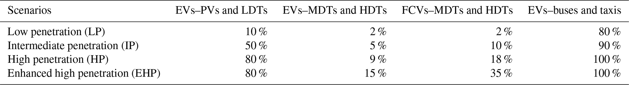
Based on high-resolution mapping of vehicle emissions, the benefits of replacing internal combustion engine vehicles (ICEVs) with new energy vehicles for emission reductions can be directly assessed. NEVs are mainly classified into battery electric vehicles (BEVs), plug-in hybrid electric vehicles (PHEVs), and fuel cell vehicles (FCVs) (Xie et al., 2024). Except for PHEVs, which emit pollutants in hybrid mode, all other NEVs produce no pollutants during driving. PHEVs only account for a relatively small proportion within NEVs (less than 20 %), and they primarily operate in electric mode during short-distance driving. Since the traffic monitoring system cannot distinguish between specific types of NEVs, all NEVs are considered zero emission in this study for simplification and uniformity. The scenario design referenced the literature review in an existing study on the environmental benefits of NEVs (Peng et al., 2021), and some adjustments were made to fit the situation in the main urban area of Jinan. Here, four scenarios of NEV penetration were set up (see Table 1), mainly oriented to passenger vehicles (PVs), trucks, buses, and taxis. Note that there is only limited research on the future NEV penetration in MDTs and HDTs, mainly due to the challenges in meeting the demands of relatively long driving ranges and addressing the problems of high costs for large-capacity rechargeable batteries and charging infrastructure (Liang et al., 2019; Secinaro et al., 2022). The government is encouraging the promotion of new energy MDTs and HDTs (China State Council, 2024), with the possibility of achieving zero-emission freight fleets in the future. However, at present most of the new energy trucks in cities are LDTs or sanitation vehicles. With consideration of the above situation, we made a bold assumption here, predicting that MDTs and HDTs will achieve a 50 % penetration in the EHP scenario. The LP, IP, HP, and EHP scenarios described the EV penetration ranges for PVs and LDTs (10 %–80 %), MDTs and HDTs (2 %–15 %), and buses and taxis (80 %–100 %), as well as the FCV penetration for MDTs and HDTs (2 %–35 %). It is noteworthy that NEV penetration in Jinan had already reached the LP level and was transitioning towards IP. NEV penetration for public transit (buses and taxis) in particular had exceeded 80 % with the active promotion of new energy policies. Nevertheless, in other cities with limited electricity supply and fewer charging devices, NEV penetration could be lower than in the LP scenario.

Table 1 New energy vehicle penetration scenarios.

3 Results and discussion

3.1 Distribution of traffic flows in the main urban area

Traffic flow is a key factor affecting on-road vehicular emissions, so it is crucial to comprehensively understand the variations in traffic flow (Deng et al., 2020). By using nearest neighbor interpolation, we generated high-resolution mapping to visualize traffic flows in the main urban area of Jinan (see Fig. 3a). The traffic flows at a fine scale (50 m×50 m) exhibited obvious spatiotemporal heterogeneities. Temporally, there were apparent diurnal variations (peak and off-peak hours) and weekly variations (weekdays and weekends) (see Fig. S1 in the Supplement). Specifically, the daytime traffic volumes were much higher than those at nighttime, accounting for approximately 81.2 % of the total. Traffic flows remained very low from 00:00 to 05:00 local time (hereafter, all times are in local time) and then started to increase at 06:00. They exhibited a bimodal pattern with two peaks appearing in the morning (07:00–09:00) and late afternoon (17:00–19:00), with a midday valley occurring at 12:00. During peak hours on weekdays in particular, the average traffic flow was 2188 vehicles h⁻¹, which was 62.4 % higher than the 24 h average. By comparison, the diurnal variation curve on weekends was smoother, with the morning peak delaying to 09:00–10:00, and the midday valley was less noticeable. In addition, weekday traffic volumes were slightly higher than those on weekends, with average traffic flows of 1367 and 1308 vehicles h⁻¹, respectively. Although commuting vehicles decreased on weekends, vehicles for leisure trips and other reasons increased, resulting in temporal dispersion. The decrease in traffic volume was mainly concentrated during the morning and late afternoon peaks. On average, the traffic flow in peak hours on weekends reached only about 90.4 % of that on weekdays.

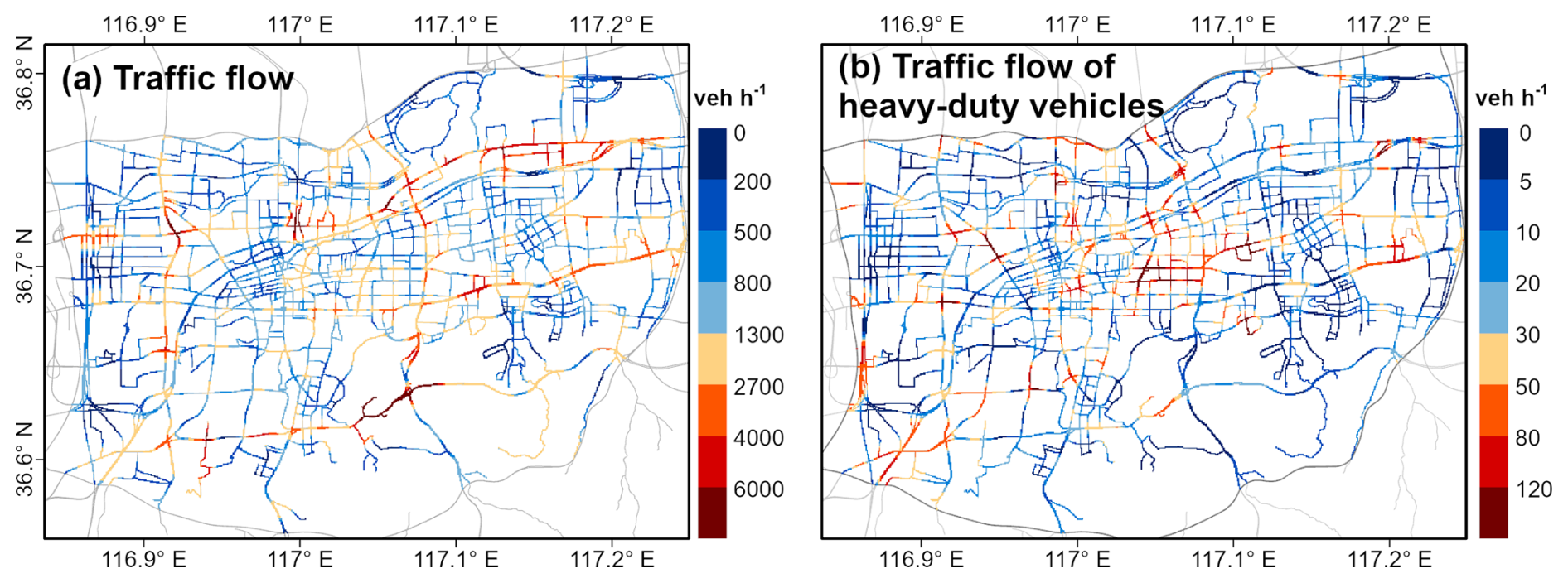
Figure 3 High-resolution mapping of hourly average traffic flows for (a) all on-road vehicles and (b) HDVs in the main urban area of Jinan.

Spatially, high-value traffic zones, defined as road segments or clusters with a traffic flow more than triple the average level ($>\mathrm{4000}\mathrm{vehicles}{\mathrm{h}}^{-\mathrm{1}}$), spread in the main urban area of Jinan. As shown by the red segments in Fig. 3a, linear high-value zones can be observed along expressways and arterial roads. Urban expressways and arterial roads carried nearly 94 % of the total traffic flows on the road network, serving as the major conduits for commuter traffic. Expressways in particular had very high traffic flows (2940 vehicles h⁻¹ on average) due to the fact that they possess multiple lanes or due to the combination of elevated and ground-level lanes. Arterial roads had moderate traffic flows, with an average value of 1093 vehicles h⁻¹. In contrast, residential areas and local streets showed quite low traffic flows ($<\mathrm{500}\mathrm{vehicles}{\mathrm{h}}^{-\mathrm{1}}$), highlighting the disparity in traffic distribution. Additionally, the traffic flows in the central business districts were substantially higher than those at the margins of urban areas, increasing the likelihood of high-value traffic zones. Furthermore, traffic flows increased sharply at intersections due to the temporary halts caused by traffic lights. It is noteworthy that when temporal peaks coincided with spatial high-value zones, the traffic flows of the high-value zones were further intensified, which is referred to as the “overlap effect of spatiotemporal peaks”. During peak traffic hours, the spatial distribution of high-value zones generally remained unchanged, but its extent expanded, and traffic flows increased (see Fig. S2 in the Supplement).

In terms of vehicle composition, as shown in Fig. S3 in the Supplement, due to the absolute dominance of LDPVs (approximately 90 %), they largely determined the spatial and temporal distribution of traffic flows. It is worth mentioning that the proportion of NEVs in the on-road vehicles approached 18 %. There was no significant difference in the fractions of various types of vehicles between weekdays and weekends, indicating relatively stable vehicle composition over the week. Except for MDTs and HDTs, all other types of vehicles primarily operated during daytime, showing a bimodal diurnal variation pattern. Regarding MDTs and HDTs, due to the stringent transportation management policy in Jinan (i.e., banning MDTs and HDTs from entering the main urban area during peak hours and from entering the area within the Second Ring Road during off-peak hours), their temporal variations and spatial distributions were different from those of other types of vehicles. There were few MDTs and HDTs other than certain municipal vehicles on the road within the urban area during peak hours. Many MDTs and HDTs drove on the roads outside the Second Ring Road during off-peak hours, with increased traffic flows at night. In addition, the high-value zone distribution of heavy-duty vehicle flows was significantly different from that of total traffic flows (as shown in Fig. 3b). As mentioned above, the total traffic flows, dominated by LDPVs, reached their maxima on expressways. In contrast, HDVs mainly operated on arterial roads, with high-value zones appearing on densely populated arterial roads in the city center.

3.2 Variation characteristics of on-road vehicle emissions

The emissions of different air pollutants from on-road vehicles in the main urban area of Jinan were calculated. The hourly average emissions of NO_x, CO, HC, and PM_2.5 were 345.2, 789.7, 69.5, and 5.4 kg, respectively. There were large variations in the contributions of different types of vehicles to each air pollutant (see Fig. S4 in the Supplement). Specifically, CO and HC were primarily contributed by LDPVs, accounting for over 60 %, which is consistent with previous studies in China (Liu et al., 2018; Sun et al., 2021; Yang et al., 2019). In addition, LDTs also contributed large portions to CO (20 %) and HC (15 %). Since both LDPVs and LDTs mainly used gasoline fuel, it can be inferred that CO and HC were mainly emitted from gasoline vehicles. In contrast, HDVs (e.g., HDTs, HDPVs, and buses) mainly used diesel fuel, and their contributions to NO_x and PM_2.5 emissions were much greater than to CO and HC emissions. For NO_x, nearly all types of vehicles (except taxis) contributed significantly to its emissions. Buses and HDTs in particular were the largest contributors (approximately 60 %) to NO_x emissions, even though they only made up less than 2 % of the traffic volume. Surprisingly, LDPVs have become the largest contributor (38 %) to PM_2.5 emissions, although their contribution was less significant in the past. On the one hand, as emission standards have become more restrictive, the differences in emission factors among LDPVs, HDPVs, HDTs, and buses have diminished (Huang et al., 2017; Sun et al., 2021). On the other hand, the volume of LDPVs is much higher than that of other vehicle types. Note that the contributions to air pollutant emissions from different types of vehicles varied among different cities in China (e.g., Beijing, Nanjing, Chongqing, and Foshan) (Wu et al., 2022; Zhang et al., 2018; Ding et al., 2021; Liu et al., 2018), mainly due to the differences in vehicle composition. For example, buses are the primary travel mode for citizens in the main urban area of Jinan. They have long routes, a necessity to maintain low to moderate speeds with frequent stop-and-go movements, and relatively high emission factors, resulting in high contributions to the emissions of NO_x and PM_2.5. Similarly, in the urban area of Beijing, buses contributed 30 % of NO_x emissions (Yang et al., 2019). Additionally, due to strict truck traffic restrictions in the urban area, the contribution of HDTs in this study was smaller than in other studies involving intercity highways (Yang et al., 2019; Zhu et al., 2023).

Vehicle emissions in urban Jinan exhibited large temporal variations, mainly caused by changes in traffic flow and vehicle composition. There were similar diurnal patterns in the emissions of CO, HC, and PM_2.5, presenting two distinct peaks in peak hours, while NO_x showed a broad peak during daytime with a small decrease in midnoon (see Fig. 4). On the one hand, the vehicle emissions of CO, HC, and PM_2.5 were dominated by LDPVs. During the peak hours in the morning and late afternoon with the highest traffic flows, the hourly emission intensities of CO, HC, and PM_2.5 also reached their peaks, with averages of 1649.4, 165.0, and 10.8 g km⁻¹, respectively. These values were 2.5–2.9 times larger than their 24 h average levels. On the other hand, NO_x emissions were dominated by HDVs for passenger and freight transport. Among them, buses and HDPVs operated in close alignment with regular schedules and daily life, primarily concentrated during daytime. In contrast, HDTs commonly flooded into the urban area during off-peak hours and midnight periods due to urban traffic restrictions, causing elevation in NO_x emissions from HDTs during off-peak periods. As a result, NO_x emissions were distributed throughout daytime, with less pronounced peaks during peak hours (see Fig. 4a). The hourly average emission intensity of NO_x during peak hours was only 66.4 % higher than the 24 h average. Generally, the unique traffic behaviors of HDVs led to disparate temporal patterns for air pollutant emissions.

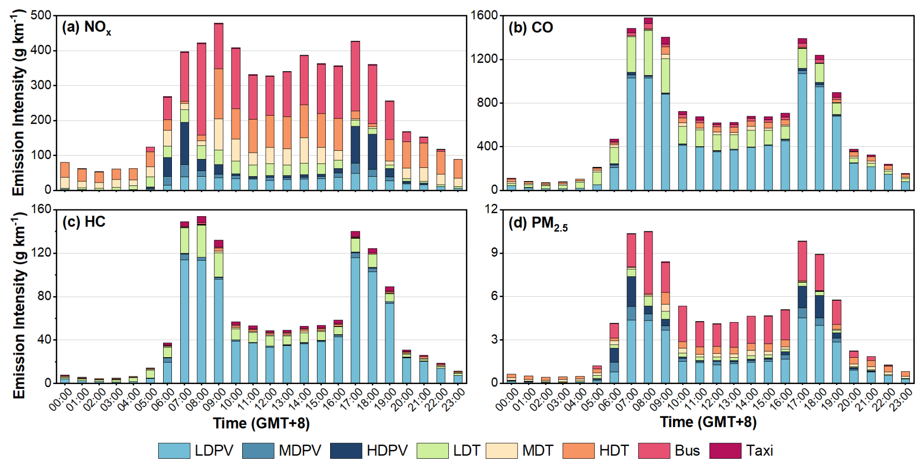
Figure 4 Average hourly emission intensities from different types of vehicles at traffic monitoring points for (a) NO_x, (b) CO, (c) HC, and (d) PM_2.5.

In addition, nearly 1 year of emission data enabled us to investigate the seasonal variations in vehicle emissions on urban roads. The monthly variation trends were generally similar for CO, HC, and PM_2.5 but a little different for NO_x, primarily determined by traffic flows and meteorological conditions. As shown in Fig. 5, traffic activities were intensified in summer (especially in July) when compared with other seasons, leading to overall higher NO_x emissions in summer. On the one hand, people preferred using cars rather than walking or cycling during the hot summer. On the other hand, summer was the peak tourist season, and many out-of-town vehicles contributed to the increased traffic volume in Jinan. Notable reductions in traffic flows and pollutant emissions were observed during Chinese official holidays, especially during National Day and Spring Festival holidays (30 September–6 October and 9–17 February). This is because human travel and commercial activities decreased, causing a sharp drop in gasoline vehicles (mainly private cars) and diesel vehicles (mainly trucks) in particular at the beginning of the holiday, followed by a gradual return to normal levels. Furthermore, the seasonal differences in vehicle emissions among different pollutants were quite pronounced due to meteorological conditions. NO_x emissions were higher in summer than in other seasons, partly owing to the high temperature during the hot season. In contrast, HC and PM_2.5 emissions peaked in winter, which is to a large degree associated with the low temperature during the cold season. High temperatures in summer affected engine combustion efficiency, leading to increased NO_x emissions. HC and PM_2.5 emissions, however, were more sensitive to low-temperature conditions and increased during cold starts due to incomplete fuel combustion. Note that the diurnal variation patterns of vehicle emissions across different seasons were similar, with high emissions occurring during daytime. Emissions in the morning (06:00–11:00) and afternoon (12:00–17:00) accounted for 41.0 % and 33.2 % on average, respectively, while those in the early morning (00:00–05:00) and evening (18:00–23:00) accounted for only 4.9 % and 20.9 %, respectively. Overall, the above seasonal and diurnal variation characteristics of air pollutant emissions from on-road vehicles provide a scientific basis for accurate air quality modeling and refined urban air pollution control.

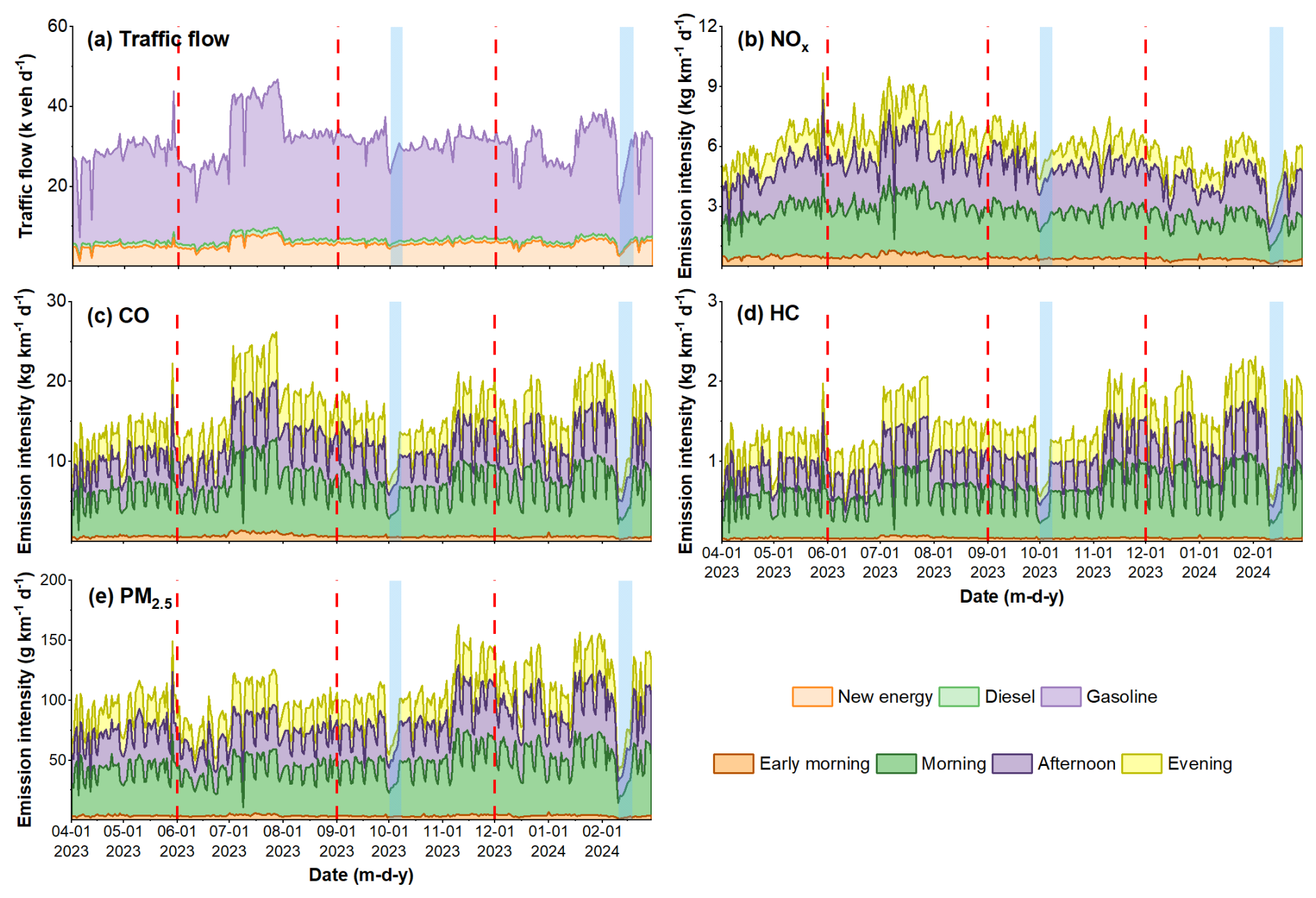
Figure 5 Daily average of (a) traffic flows for different types of vehicles and emission intensities of (b) NO_x, (c) CO, (d) HC, and (e) PM_2.5 during different time periods of the day. The dashed red lines represent the division by seasons, while the blue bars represent official holidays.

Spatially, the distribution characteristics of air pollutant emissions from on-road vehicles were strongly associated with traffic flow distributions (see Fig. 6). This variation pattern differs to some degree from previous results, which generally show a decrease from the urban center to the periphery in a radiating structure (Zhang et al., 2018; Yang et al., 2019). Firstly, HDVs dominated NO_x and PM_2.5 emissions, and their spatial distributions exhibited similar characteristics to the distribution of heavy-duty vehicle flows, with high-emission zones (hourly emission $\text{intensity}>\mathrm{850}\mathrm{g}{\mathrm{km}}^{-\mathrm{1}}$) primarily appearing on arterial roads in the city center. LDVs dominated CO and HC emissions, thus considerably influencing their spatial distributions, with linear high-emission zones observable along urban expressways. Therefore, influenced by the dominant types of vehicles, the spatial distributions of vehicle emissions in urban Jinan varied for different air pollutants, which is consistent with a previous study by Sun et al. (2021). Secondly, grids with high emissions were predominantly located at urban expressways or the intersections of arterial roads. In contrast, grids with low emissions were generally situated on residential streets and urban peripheries with relatively low traffic volumes. The average traffic flows on urban expressways, highways, arterial roads, secondary roads, and local streets followed a descending order, with the emission intensities following the same decreasing trend. For instance, the calculated hourly average NO_x emission intensities on urban expressways, highways, arterial roads, secondary roads, and local streets were 485.1, 303.4, 240.8, 84.2, and 74.6 g km⁻¹, respectively. Among the four types of roads, arterial roads had the longest length with the largest traffic volume, accounting for 48.4 % of the total, while the corresponding emissions contributed 54.9 % of the total emissions. Urban expressways carried 45.6 % of the total traffic volume, but their emissions amounted to only 38.7 %. The primary reason for this discrepancy is the difference in vehicle compositions across different types of roads; i.e., the volume of HDVs on arterial roads was up to 35.6 % higher than that on urban expressways. As a result, although vehicle compositions were independent of the distribution of traffic flows, they largely affected the emission distribution characteristics, particularly over fine-scale areas. In addition, Fig. 6 shows that high emissions frequently appeared in intersections, with emission intensities radiating from the intersection to the surrounding roads. This feature has rarely been presented in other high-resolution vehicle emission mappings (Jiang et al., 2021; Wu et al., 2022), but in this study, interpolation makes the differences between intersections and road segments more pronounced (see Fig. S5 in the Supplement). The emissions within 1 km of an intersection varied significantly, by a factor of 1.4–3.

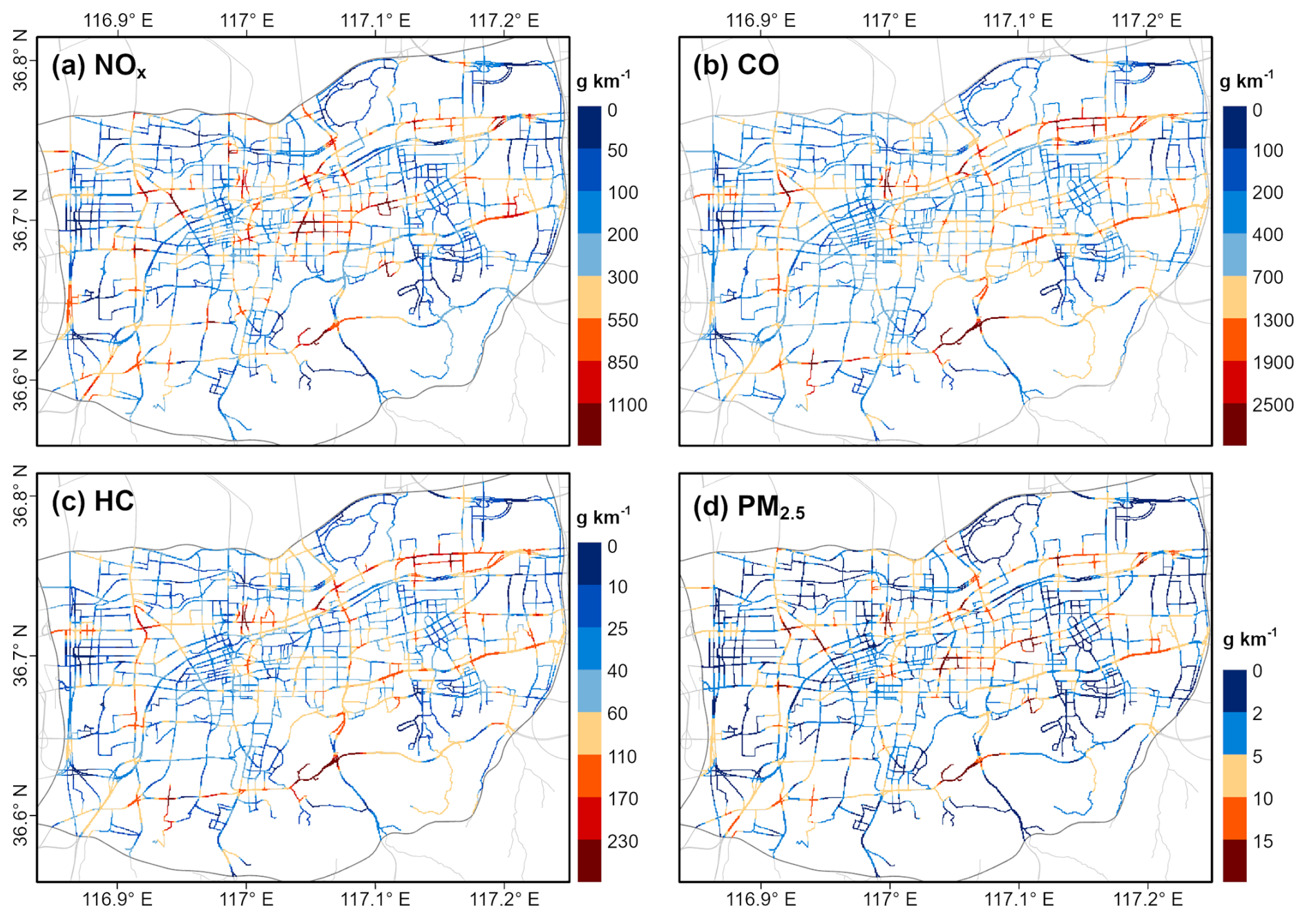
Figure 6 High-resolution mapping of hourly average vehicle emission intensities of major pollutants, including (a) NO_x, (b) CO, (c) HC, and (d) PM_2.5, in the main urban area of Jinan.

Figure 7 uses NO_x as an example to show the spatial distributions of vehicle emissions during different time periods in the main urban area of Jinan, aiming to explore the emission patterns under the joint influence of temporal and spatial characteristics. Firstly, the vehicle emissions during daytime were significantly higher than those at nighttime, with daytime emissions contributing more than 74 % of the total NO_x emissions. During the early morning, there were virtually no high values distributed across urban Jinan (as shown in Fig. 7c). Secondly, the emissions during the short peak hours accounted for approximately 37 % of the daytime emissions on weekdays, with high-emission zones accounting for 14.7 %. Note that the overlap effect of spatiotemporal peaks observed in traffic flow mapping could also be seen in the mapping of vehicle emissions. For example, the spatial distribution of vehicle emissions during peak hours (see Fig. 7a) remained generally unchanged when compared to off-peak hours (see Fig. 7b). However, the high-emission zones (red lines in Fig. 7a and b) expanded significantly on the original basis, with the hourly average emission intensity increasing by 1150 g km⁻¹. In contrast, roads with initially low emissions (blue lines in Fig. 7a and b, hourly emission $\text{intensity}<\mathrm{100}\mathrm{g}{\mathrm{km}}^{-\mathrm{1}}$) only showed an increase of 63.4 g km⁻¹ in hourly emission intensity during the peak hours, with most still remaining at low levels. Thirdly, the spatial distributions of vehicle emissions on weekdays and weekends were generally consistent, with slightly higher emission levels on weekdays than on weekends (292.3 vs. 247.9 g km⁻¹ in the hourly average emission intensity) (see Fig. 7f). All in all, the above spatial variation patterns of NO_x emissions from on-road vehicles were closely related to regular commuting and the lifestyle of residents, and the same applied to the other three pollutants (see Figs. S6–S8 in the Supplement).

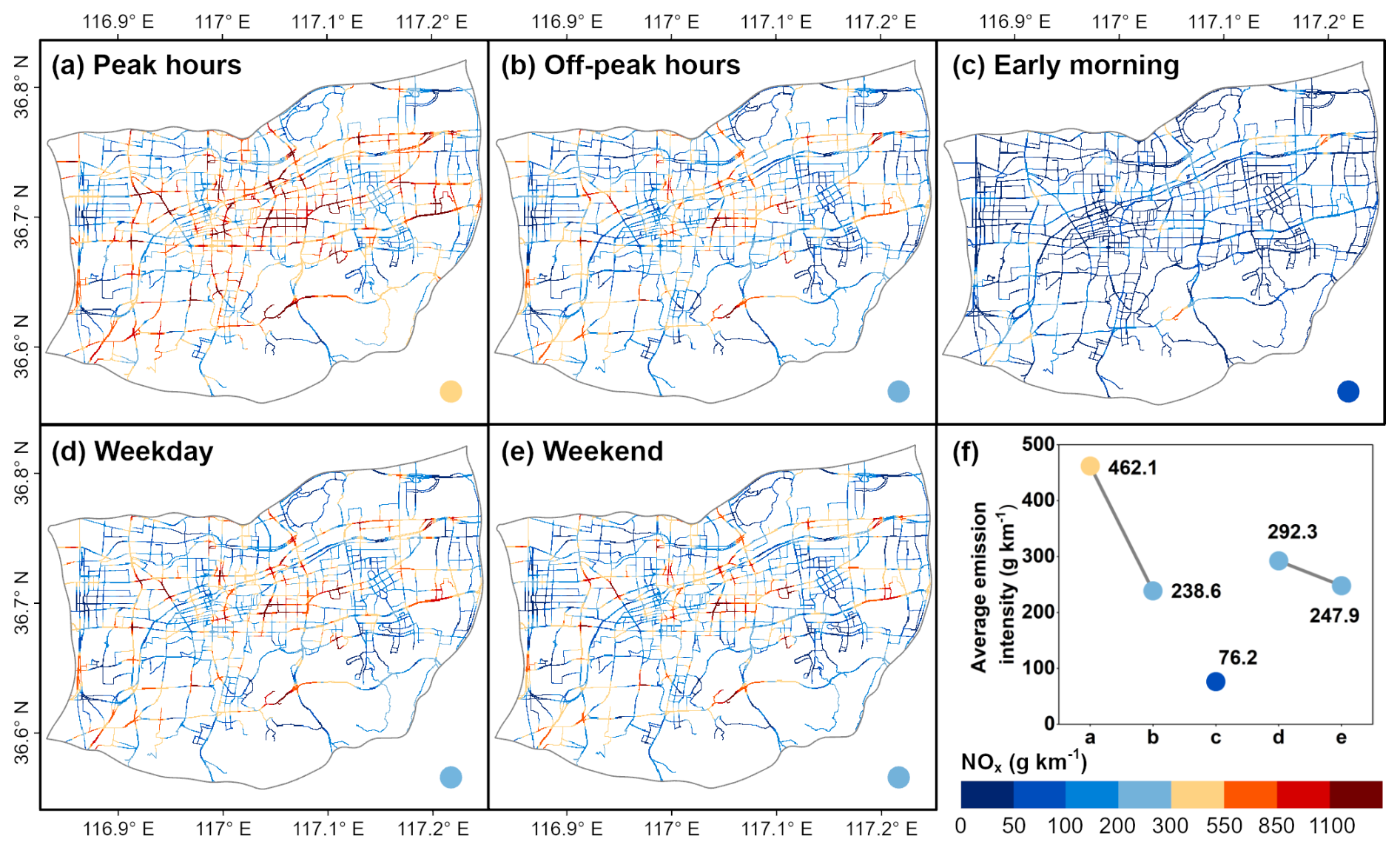
Figure 7 High-resolution mapping of on-road vehicle NO_x emissions during (a) peak hours, (b) off-peak hours, (c) early morning, (d) weekdays, and (e) weekends and (f) average emission intensities of NO_x during each time period.

3.3 Temporal and spatial cluster characteristics of vehicle emissions

To further understand the spatiotemporal variation behaviors and the main influencing factors of vehicle emissions, temporal and spatial clustering analyses were conducted with the hourly vehicle emission data for four pollutants. Based on the results from time series clustering, the optimal number of clusters (K) was determined as 2, with the highest silhouette coefficient and two distinct diurnal variation patterns. As shown in Fig. 8a and c, CO and HC emissions in Cluster 1 were concentrated during peak traffic hours in the morning and late afternoon, with emission intensities dropping sharply after the peaks. Additionally, NO_x and PM_2.5 emissions in Cluster 1 also showed two distinct peaks during peak hours. In contrast, the diurnal emission plots for four air pollutants in Cluster 2 were relatively smooth, with no distinct peaks, and the differences were only evident between daytime and nighttime (see Fig. 8b and d). The fluctuation degrees of diurnal emissions for each pollutant in the two clusters were calculated by using the coefficient of variation (CV), and it was found that the average CV of Cluster 1 was 82.5 %, much higher than that of Cluster 2 (55.5 % on average). Furthermore, the emission levels of the two clusters were similar, with NO_x and CO emissions in Cluster 2 slightly higher than those in Cluster 1 (by 26.5 % and 12.7 %, respectively). Figure 8e visually shows the spatial distributions of the two clusters, showing the areas affected by different emissions patterns. It was evident that most traffic monitoring points on urban expressways and highways belonged to Cluster 2. These roads were mainly used for long-distance travel and fast passage and did not experience large-scale traffic congestion during peak hours. In addition, vehicles on elevated roads maintained high speeds and uniform traffic flows, with few stops due to traffic lights or congestion, resulting in evenly distributed emissions throughout the day. Some residential roads with low traffic volumes were also classified as Cluster 2. Instead, Cluster 1 was mainly distributed on arterial roads, intersections, and near commercial areas within the city, where vehicles were dense during peak hours, leading to sharp increases in emissions due to the overlap effect of spatiotemporal peaks. As a result, the diurnal variation in vehicle emissions was not uniform across roads with different characteristics, indicating spatial instability. This has not received much attention in previous studies, which typically considered the entire region as a whole and revealed only bimodal patterns (Jiang et al., 2021; Ding et al., 2023).

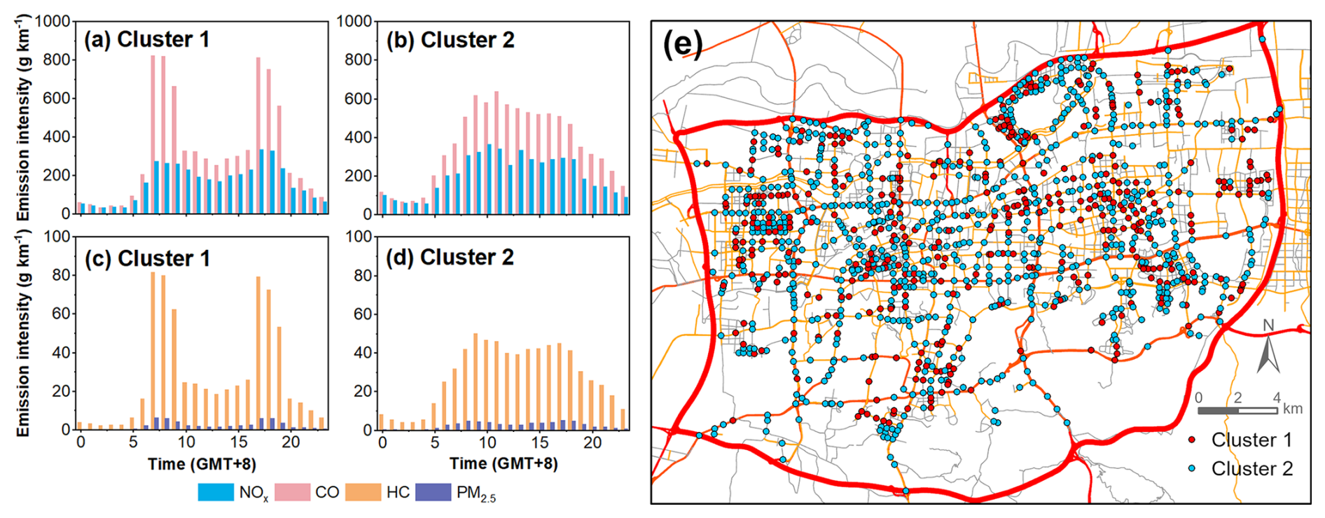
Figure 8 Hourly average emission intensities of NO_x and CO for (a) Cluster 1 and (b) Cluster 2, hourly average emission intensities of HC and PM_2.5 for (c) Cluster 1 and (d) Cluster 2, and (e) the distributions of traffic monitoring points belonging to different clusters in the main urban area of Jinan.

The findings on the diurnal variation patterns of vehicle emissions and the corresponding spatial distribution characteristics provide scientific recommendations for emission reduction measures and resident travel. For example, controlling the traffic volume during peak hours is required on arterial roads to reduce traffic congestion and high emissions of air pollutants. On expressways, ensuring unblocked traffic and improving transit efficiency are particularly important. Regarding resident travel, it is recommended to avoid major arterial roads and other easily congested areas during peak hours by traveling earlier or later. Residents can also use public transportation, ride bicycles, or walk as alternative modes of travel. In addition, choosing expressways with high traffic efficiency is advisable. While driving on expressways, maintaining a steady speed and avoiding frequent lane changes and sudden acceleration or braking can improve fuel efficiency and reduce pollutant emissions.

Spatial clustering characteristics of vehicle emissions were obtained through hotspot analysis by calculating the Getis–Ord $G_i^{\ast }$ statistics. The locations and potential causes of clustering for high- or low-value features were identified at a fine scale (see Fig. 9). The emission hotspots for different pollutants were likely driven by different factors, including high traffic volumes, concentrated HDVs, and road intersections (see Fig. S9 in the Supplement). Specifically, NO_x and PM_2.5 emission hotspots were dominated by HDVs, clustered along densely trafficked arterial roads in the city center, while cold spots mostly appeared in residential areas (see Fig. 9a and d). There was a huge difference in the emissions between hotspots and cold spots. For example, the hourly average NO_x emission intensity on Heping Road (hotspot area) was 2557.9 g km⁻¹, which was 172 times higher than that on Xingfusi Road (cold spot area, 14.9 g km⁻¹ on average). In addition, CO and HC emissions usually peaked on urban expressways with high traffic volumes, forming linear hotspot areas (see Fig. 9b and c). Their highest emission was found on the South Second Ring Elevated Road, which had the highest traffic volume (see Fig. 3a). Furthermore, the emission hotspots remained spatially stable, showing similar levels from day to day. However, due to the overlap effect of spatiotemporal peaks, the emission intensities at hotspot areas varied over time during the day, with peaks typically appearing around 08:00 in the morning and 18:00 in the late afternoon on weekdays.

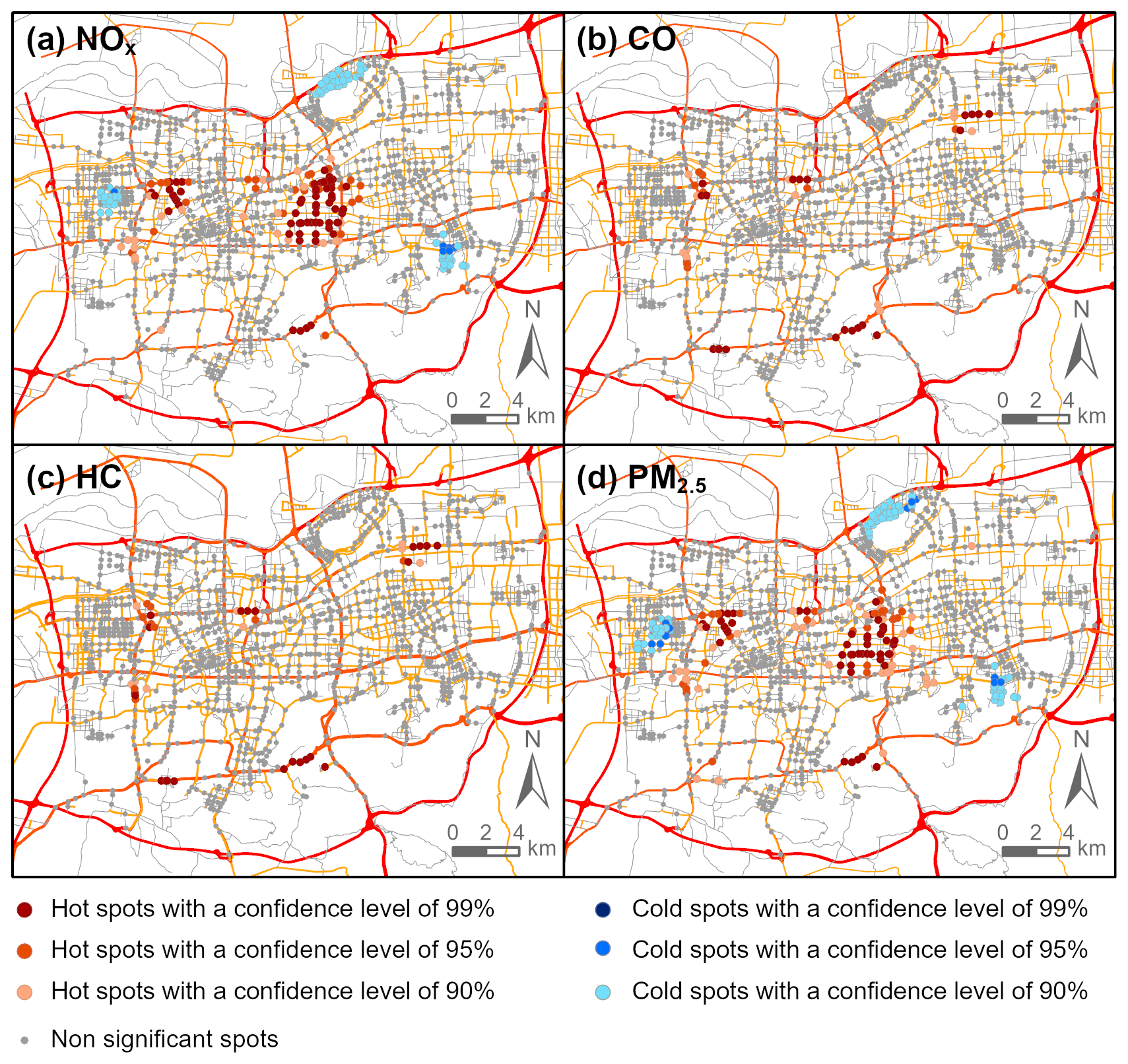
Figure 9 Spatial distributions of hotspots and cold spots of on-road vehicle emissions for (a) NO_x, (b) CO, (c) HC, and (d) PM_2.5.

Overall, both the temporal and the spatial clustering analyses suggest that only a small number of vehicles and roads contributed very high emissions, while the majority exhibited relatively low emissions. The phenomenon that high-emission vehicles and roads made notable contributions to the total emissions is consistent with the finding reported by Böhm et al. (2022). Therefore, effective policies for vehicle emission reduction should primarily focus on key time periods, key areas, and key types of vehicles. For instance, differentiated traffic restriction measures can be implemented based on the dual-peak emission characteristics in the morning and late afternoon. Introducing new energy public transportation in identified high-emission time periods and areas will reduce the use of private vehicles. Utilizing real-time traffic data to intelligently adjust signal timing can help adapt to peak and off-peak traffic periods, thereby minimizing congestion and pollutant emissions (Yang et al., 2020). Implementing a low-emission-zone policy to restrict high-emission vehicles from entering the city center is also recommended.

3.4 Impacts of new energy vehicle replacement

Due to policy support, environmental benefits, technological advancements, and cost reductions, the number of new energy vehicles in China has been growing rapidly in recent years (Zhang et al., 2023). According to statistics (MPS, 2024), 7.43 million NEVs were newly registered in 2023, accounting for 30.2 % of the total number of newly registered vehicles. NEVs can reduce the emissions of air pollutants from vehicles and subsequently improve urban air quality. Therefore, it is necessary to assess the specific emission reduction benefits brought by vehicle electrification with assumptions of suitable future penetration of NEVs. In this paper, the current emission levels in the main urban area of Jinan were used as the base case. Since the LP scenario was very close to the current situation of the city, it was not presented in detail in this study. Three scenarios, including IP, HP, and EHP, reflect discrepant electrification penetration for different types of vehicles. Specifically, the IP and HP scenarios comprehensively increase the penetration of NEVs across various vehicles. In particular, large fractions of LDVs will be replaced with NEVs as they contribute significantly to on-road vehicle emissions. For the HDVs, which have high emission factors, the electrification of buses has been successful, whereas the transformation of trucks has faced challenges and has proceeded slowly. In addition, we designed the EHP scenario, which further increases NEV penetration of MDTs and HDTs to achieve more appreciable emission reduction benefits (Böhm et al., 2022; Tian et al., 2022).

Figure 10 shows the on-road emission intensities for NO_x, CO, HC, and PM_2.5 in the main urban area of Jinan under different future scenarios and the reductions compared with current emissions. Specifically, under the IP scenario, vehicle emissions decreased by large amounts, i.e., 42.7 % for NO_x, 39.1 % for CO, 40.3 % for HC, and 50.1 % for PM_2.5, when compared with the present emission intensities, and most of the emission hotspots disappeared. For the HP scenario, which involved a further increase in NEV penetration, this led to significant additional reductions in emissions, particularly on urban expressways and arterial roads; i.e., NO_x decreased by 23.4 %, CO by 34.0 %, HC by 34.8 %, and PM_2.5 by 27.0 % relative to the IP scenario. At that time, emission hotspots on all roads were virtually eliminated, indicating the positive impact of comprehensive vehicle electrification on road vehicle emissions, especially in the city center. Surprisingly, in the EHP scenario, where we increased the NEV penetration of MDTs and HDTs to 50 %, emissions were further reduced by an average of only about 2.5 %. Among them, NO_x emissions, which were most affected by MDTs and HDTs, showed the highest reduction of 5.9 %. As mentioned above, within the traffic restrictions in the main urban area, the proportion of MDTs and HDTs in urban areas was very small (only 2 %), and their emissions only contributed a small fraction to the total vehicle emissions. Consequently, the reduction in on-road vehicle emissions was not significant under the EHP scenario.

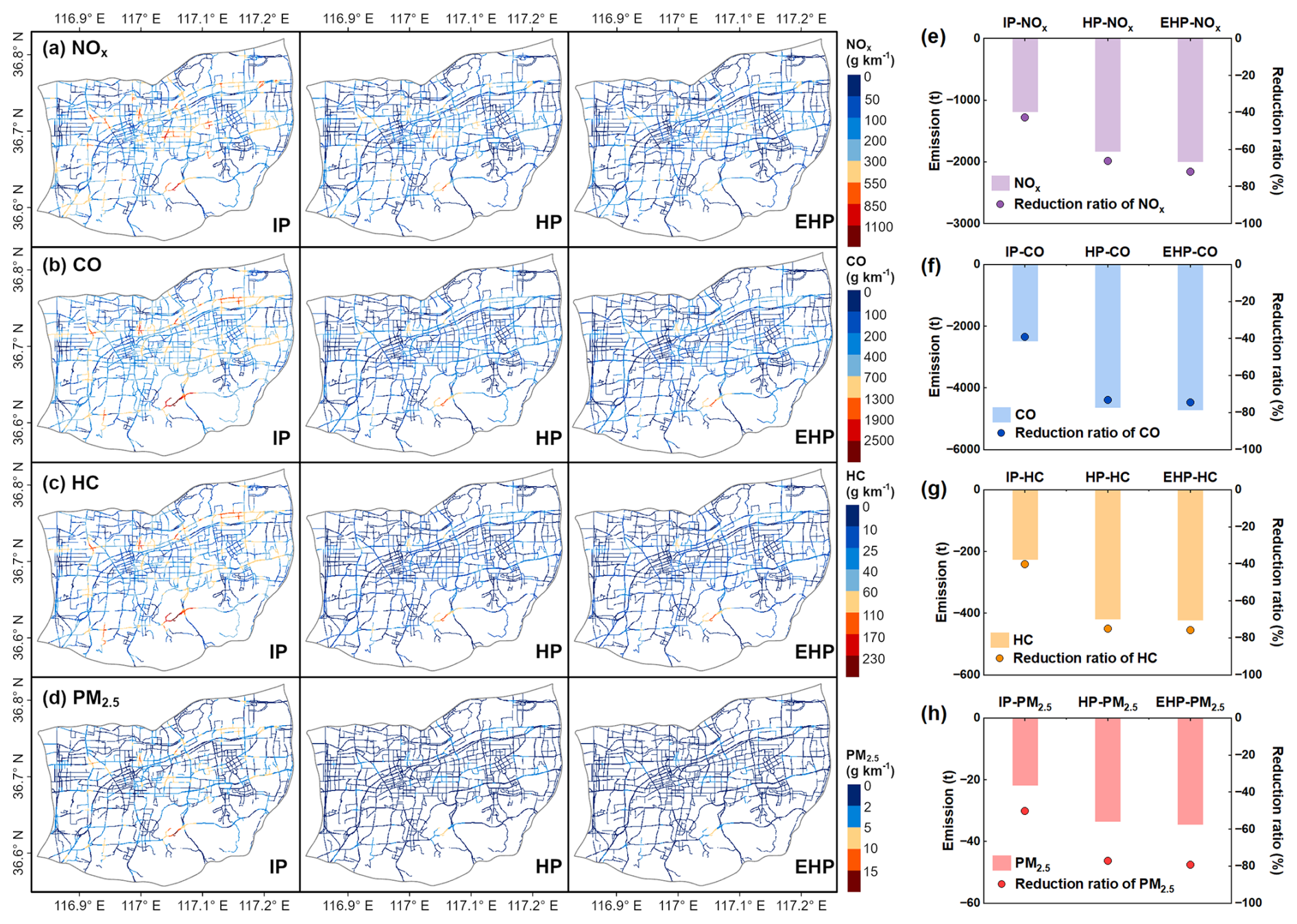
Figure 10 On-road vehicle emission mappings for (a) NO_x, (b) CO, (c) HC, and (d) PM_2.5 simulated under different new energy penetration scenarios and emission reductions for (e) NO_x, (f) CO, (g) HC, and (h) PM_2.5 under each scenario relative to the base case during the study period. The bars indicate the emission reduction amounts, and the dots indicate the percentage reduction.

Note that when evaluating the impact of NEV penetration on on-road vehicle emissions, our calculations and analyses were based merely on exhaust emissions, focusing on the differences in exhaust emissions between ICEVs and NEVs. However, a substantial portion of PM emissions were contributed by non-exhaust sources (e.g., road dust, brake wear, and tire wear) (Zhang et al., 2020). Additionally, NEVs are typically heavier than conventional vehicles, which may lead to higher non-exhaust emissions (Timmers and Achten, 2016; Liu et al., 2021). Therefore, if the contribution of non-exhaust emissions was also taken into account, the estimated benefits of increased NEV penetration on reducing PM_2.5 emissions would be lower than suggested by our current analysis.

3.5 Comparison with other vehicle emission inventories

To verify the reliability of the high-resolution emission inventories of on-road vehicles in the main urban area of Jinan obtained in this study, comparisons with other limited emission inventories from previous studies were conducted. Firstly, Feng et al. (2023) established a high-resolution vehicle emission inventory for NO₂ and CO in Jinan for the year of 2021 by using a top-down approach with a resolution of 1 km×1 km. Their results showed similar spatial distribution patterns to our study; i.e., the high-emission zones were concentrated in the city center or near high-grade roads, with notably higher pollutant emissions in Lixia District compared to other areas. Nevertheless, due to the lack of dynamic traffic data, their inventory failed to present the fine-scale gradients of on-road vehicle emissions. Second, from the Multi-resolution Emission Inventory for China (MEICv1.4) with a low resolution of 0.25°×0.25° for 2020 (Zheng et al., 2014), there were only two grids in the main urban area of Jinan (see Fig. S10 in the Supplement). When compared with the re-aggregated total emissions from gasoline and diesel vehicles in MEICv1.4, the monthly average air pollutant emissions of on-road vehicles obtained in our study were significantly lower, with ratios of 58.1 % for NO_x, 28.5 % for CO, 12.3 % for HC, and 51.2 % for PM_2.5. The main reason for the apparently low HC was that the evaporative emissions of HC were excluded in this study. In addition, the continuous implementation of emission reduction measures, including elimination of high-emission vehicles, improvement in fuel quality and emission standards, and promotion of NEVs over the past 3 years, also contributed to the lower emissions in our study.

4 Summary and conclusions

This study developed a high-resolution on-road vehicle emission inventory for the main urban area of Jinan by using a bottom-up approach based on a large amount of real-world traffic data collected in real-time from more than 1000 traffic monitoring points. Fine-scale traffic flows and vehicle compositions over approximately 1 year were gathered with extensive traffic cameras and field surveys to calculate the emission intensities from different types of vehicles. Multiple big data methods were utilized to demonstrate the temporal and spatial variation patterns of vehicle emissions with the massive traffic dataset. Specifically, nearest neighbor interpolation and Gaussian smoothing were used to fill in spatial data gaps to obtain spatially continuous vehicle emission maps in an ultra-high resolution of 50 m. Through time series clustering and hotspot analysis, the spatiotemporal clustering characteristics of vehicle emissions were analyzed, and travel recommendations for residents were provided. The benefits of vehicle emission reduction with increased NEV adoption in the future were predicted at three potential scenarios with different NEV penetration levels.

Results show that the daily average on-road vehicle emissions in the main urban area of Jinan were 8.28, 18.95, 1.67, and 0.13 t for NO_x, CO, HC, and PM_2.5, respectively. Among the different types of vehicles, the contributions of HDTs to pollutant emissions were relatively small (2 %–23 %) due to strict traffic restrictions in the main urban area. The contribution of buses was slightly large (1 %–34 %), demonstrating the importance of further promoting the electrification of public transportation in Jinan. The variation in vehicle emissions was strongly affected by traffic activities, primarily occurring during daytime, with the highest emission intensities during peak hours (2.5–2.9 times as high as the hourly average levels). The emissions of air pollutants of CO, HC, and PM_2.5 exhibited distinct bimodal diurnal patterns, primarily contributed by LDPVs with contributions of 38 %–74 %. In contrast, 66 % of NO_x emissions were caused by HDVs, which were distributed throughout the day with less pronounced peaks during peak hours. The emission hotspots of CO and HC were linearly distributed along urban expressways with high traffic volumes, whereas those of NO_x and PM_2.5 were mainly concentrated on arterial roads in the city center where there were more HDVs. The overlap effect of spatiotemporal peaks was in particular observed in on-road vehicle emissions in urban Jinan. When the temporal peaks coincided with the spatial hotspots, the emissions were further intensified. During peak hours, the high-emission zones expanded significantly, with the hourly average NO_x emission intensity increasing by 1150 g km⁻¹, while the low-emission zones only showed an increase of 63.4 g km⁻¹. In addition, on-road vehicle emissions exhibited notable seasonal differences, with higher NO_x emissions in summer but higher HC and PM_2.5 emissions in winter. Furthermore, the simulations of NEV penetration scenarios indicate that the electrification of vehicles has large impacts on vehicle emissions and their spatial patterns. There were reductions of 40 %–80 % in emissions, and most hotspots disappeared in the future. These results not only demonstrate the potential of fleet electrification in emission reduction, but also provide a scientific basis for formulating more precise emission reduction strategies.

More importantly, the framework of high-resolution vehicle emissions developed in this study applies to almost any other city. Once traffic monitoring and road network data with full coverage are provided, it can support decision-makers in implementing emission reductions, improving citizen welfare, and designing strategies for more sustainable cities. As more traffic data become available in the future, research can be extended to include the surrounding suburban and rural areas. Additionally, the potential of big data techniques in establishing emission inventories can be further explored to establish a dynamic big data platform that integrates multiple sources, such as traffic cameras, low-cost sensors, GPS data, and open-source congestion maps. Machine learning (ML) can further enhance the framework by dynamically optimizing emission factors based on traffic patterns, vehicle types, and meteorological conditions, thereby achieving real-time traffic data processing and dynamic updates to vehicle emission inventories.