An investigation of the impact of Canadian wildfires on US air quality using model, satellite, and ground measurements

Canadian wildfires transport large concentrations of particulate matter into the US, leading to various effects on the surface temperature, the radiation balance, and visibility and exacerbating pollution-related respiratory conditions. Using a combination of surface, satellite, and numerical models, this study quantifies the increase in surface fine particulate matter (PM_2.5) in the continental US due to long-range transported smoke from Canadian wildfires during a wildfire episode from 9–25 August 2018. As a widely used indicator of surface pollution levels, satellite-retrieved aerosol optical depth (AOD) can provide crucial information on columnar pollution mass. However, the daily spatial coverage of satellite AOD is restricted due to cloud cover. In order to quantify the daily changes in surface pollution, we fill in the AOD gaps by utilizing simulated 10 km spatial resolution AOD from a chemistry transport model (CTM). Meteorological variables influencing smoke transport were also integrated alongside the gap-filled AOD product to estimate surface PM_2.5 using geographically weighted regression (GWR) and random forest (RF) models. The model with better performance was subsequently applied to quantify PM_2.5 changes due to Canadian wildfires. To isolate the impact of Canadian wildfires, we calculate the surface PM_2.5 ratio with and without Canadian fire sources by conducting two CTM simulations: one with Canadian wildfire emissions enabled and another with these emissions turned off. Our results show that Canadian wildfires caused a significant increase in surface PM_2.5, contributing up to 28 µg m⁻³ (a 69 % increase) across different US Environmental Protection Agency (EPA) regions during the August 2018 wildfire event.

1 Introduction

Airborne fine particulate matter (PM_2.5), with aerodynamic diameters less than 2.5 µm, is a well-documented contributor to increased mortality from diseases such as ischemic heart disease, chronic obstructive pulmonary disease, cardiovascular disease, respiratory disease, lung cancer, chronic kidney disease, hypertension, and dementia (Chen and Hoek, 2020; Bu et al., 2021; Bowe et al., 2019). In 2017, PM_2.5 exposure was linked to 4.58×10⁶ deaths globally, with ambient PM_2.5 accounting for 64.2 % of these deaths (Bu et al., 2021). PM_2.5 originates from diverse sources, including combustion processes, power plants, dust, sea salt, and secondary chemical reactions. In the US, wildfires are a significant and growing source of PM_2.5 pollution (O'Dell et al., 2019). For regions affected the most by wildfires, like the state of Washington (WA), an increase in daily PM_2.5 of 97.1 µg m⁻³ during the summer of 2020 was found, which was related to 92 more mortality cases (Liu et al., 2021). Moreover, the toxicity of PM originating from wildfire smoke has been found to be 3–4 times greater than equivalent doses of ambient PM (Wegesser et al., 2009). Health impacts vary with chemical composition, which depends on biomass combustion stages and temperature (Kim et al., 2018; Aguilera et al., 2021). Beyond its health impacts, wildfire-related PM_2.5 imposes considerable economic burdens. From simulation results, wildfire-related economic costs have been projected to increase from USD 7×10¹²–43×10¹² per year in 2090 (Neumann et al., 2021).

Given the growing role of wildfires as a major PM_2.5 source, accurately assessing pollution levels requires understanding the transport dynamics and chemical transformations of wildfire smoke, which are influenced by factors such as fire intensity, injection height, atmospheric dynamics, and terrain interactions. Higher fire radiative power (FRP) results in longer distances of the smoke transport due to higher plume injection heights (Solomos et al., 2015). A global analysis of over 23 000 wildfires found that significant injection heights going into the free troposphere are primarily observed in the boreal forests of North America and Siberia during the Northern Hemisphere summer (Val Martin et al., 2018). Smoke remnants from Canadian stand-replacing forest fires have been observed at altitudes exceeding 13 km (Damoah et al., 2006). Once injected, smoke plumes can descend to the surface through a combination of subsidence, interception, and diurnal entrainment within the planetary boundary layer (PBL), as observed in the eastern US for the July 2002 Canadian forest fire event (Colarco et al., 2004). Atmospheric circulation plays a key role in shaping smoke transport. Upper-level winds facilitate long-range horizontal transport, while surface high-pressure systems enhance ground-level pollution through subsidence inversions (Miller et al., 2011). Cyclonic circulation can form a multilayer PBL, characterized by temperature inversions and stable stratification, which trap pollutants in convergent zones (Jiang et al., 2021b). Interactions with mountain terrain further modulate smoke dispersion: under stable synoptic conditions, valleys become more stagnant, while unstable conditions promote vertical mixing (Beaver et al., 2010; Lang et al., 2015). During transport, smoke particles undergo physical and chemical transformations that influence their sizes, such as hygroscopic growth (Carrico et al., 2005; Gomez et al., 2018), secondary organic aerosol (SOA) formation (Ahern et al., 2019), condensation of semi-volatile species (Reid et al., 2005; Zhou et al., 2017; Akagi et al., 2012), and coagulation process (Aloyan et al., 1997; Sun et al., 2019).

Estimating surface PM_2.5 concentrations presents significant challenges due to spatial and temporal variability and limited ground station coverage. Traditional approaches, such as spatial interpolation (e.g., inverse distance weighting, ordinary Kriging) rely primarily on ground-based PM_2.5 measurements, while linear regression methods combine satellite-derived aerosol optical depth (AOD) with surface PM_2.5 measurements (Hoff and Christopher, 2009). More advanced methods, like multi-linear regression, typically incorporate surface PM_2.5 data, satellite AOD, and meteorological datasets from models (Gupta and Christopher, 2009b). Geographically weighted regression (GWR) and machine learning methods use data sources similar to multi-linear regression but offer better spatial resolution and adaptability to local variations (Xue et al., 2021; Ma et al., 2014; Bai et al., 2016; Song et al., 2014; Hu et al., 2017; Gupta and Christopher, 2009a; Zamani Joharestani et al., 2019). Linear mixed-effect models add temporal variability by including both fixed and random effects (Ma et al., 2016; Lee et al., 2011). Chemistry transport models (CTMs) leverage detailed atmospheric chemistry and physics simulations using emission inventories, meteorological fields, and chemical species distributions (Geng et al., 2015; Xue et al., 2019). Traditional methods like spatial interpolation and linear regression struggle to integrate multiple mechanisms and spatiotemporal variables, a limitation newer techniques address (Zhang et al., 2018). Due to the growth of computing power, machine learning (or artificial intelligence) has become a major focus for estimating the spatiotemporal dynamic distribution of surface PM_2.5 concentrations (Zhang et al., 2018; Sayeed et al., 2022).

Satellite-retrieved AOD serves as a valuable indicator of columnar pollution, providing critical information for estimating surface PM_2.5 concentrations, though it is not a direct measurement of surface pollution (Wang and Christopher, 2003; Geng et al., 2015). Its key advantages include over 2 decades of data availability from polar-orbiting sensors and the extensive spatial coverage of satellite observations, making it a powerful tool for long-term air quality analysis. However, cloud cover frequently obstructs AOD retrievals, limiting their utility for daily surface PM_2.5 estimation (Goldberg et al., 2019). To overcome this limitation, gap-filling methods are used to generate spatially and temporally continuous AOD datasets. These methods include fusing retrievals from multiple satellite sensors (Ma et al., 2014); applying multiple imputation techniques using auxiliary data such as cloud fraction, elevation, and humidity (Xiao et al., 2017); and using statistical approaches like Kriging to interpolate AOD based on seasonal and regional AOD : PM_2.5 ratios derived from ground-based measurements (Lv et al., 2017). Additionally, incorporating chemistry transport model (CTM) simulations into the gap-filling process has been shown to significantly improve the accuracy and reliability of imputed AOD values (Xiao et al., 2021). The AOD–PM_2.5 relationship is influenced by aerosol composition, vertical distribution, and meteorological factors. The boundary layer height (BLH) serves as a key indicator by representing the mixing height of aerosols and their influence on surface pollution levels (Gupta and Christopher, 2009b). Surface pressure also plays a role, with high-pressure systems linked to surface pollution increases due to subsidence inversions (Miller et al., 2011). Additionally, relative humidity (RH) affects this relationship, as AOD is sensitive to particle size and hygroscopic growth (Li et al., 2014), while PM_2.5 reflects dry mass. Incorporating these meteorological parameters helps models better capture the dynamic processes shaping the AOD–PM_2.5 relationship.

This study is designed to assess the pollution change due to fine particulate matter in the US transported by smoke from Canadian wildfires and to also examine the physical processes during transport that affects surface pollution along the path. First, by turning on and off the fire emissions in the CTM in Canada, we conduct two WRF-Chem (Weather Research and Forecasting model coupled with Chemistry) simulations to investigate the processes that influence the transport of remote smoke aerosols in the atmosphere. According to the analysis of different processes, we then selected variables associated with smoke's vertical distribution, which determined the relationships between AOD and surface pollution concentrations. Finally, by filling in the satellite AOD gaps due to cloud covers using CTM simulations, we estimate the surface pollution increase due to the remote fires using the filled AOD along with surface PM_2.5 measurements and other meteorological variables.

2 Data and study area

2.1 Study area

We estimated daily mean surface PM_2.5 at 0.1° spatial resolution over the continental US (CONUS) from 9–25 August 2018. The study area (inner domain) focuses on the US (25–50° N, 64–125° W), while the outer domain of the same WRF simulation extends to Canada (25–67° N, 70–140° W) to account for Canadian fire emissions and their contributions to US pollution from remote fire sources. Therefore, we chose August 2018 as our study period to analyze the impact of wildfires on surface air pollution in the US based on the total fire radiative power calculation based on our previous work (Xue et al., 2021).

2.2 Ground-level PM_2.5 observations

We obtained the daily surface PM_2.5 concentration product that uses Federal Reference Methods (FRMs) and Federal Equivalent Methods (FEMs) (code 88101) from the US Environmental Protection Agency (EPA) for CONUS within the study period (https://www.epa.gov/outdoor-air-quality-data/, last access: 24 May 2025). The measured frequency of each site is different (with a measurement interval of every 1, 3, or 6 d). A total of 950 EPA sites are available with approximately 71.1 % sampling for daily data within the study period. Note that we discarded all PM_2.5 values lower than the established detection limit of 2 µg m⁻³ (EPA, 2018).

2.3 Satellite data

AOD values retrieved from satellite observations, which are a columnar value of aerosol extinction, are correlated with surface pollution under certain conditions (Wang and Christopher, 2003; Hoff and Christopher, 2009). The relation between AOD and surface PM_2.5 can be expressed as the following equation (Koelemeijer et al., 2006):

$$\begin{array}{}\text{(1)}& {\displaystyle }{\displaystyle }\text{AOD}={\mathrm{PM}}_{\mathrm{2.5}}Hf\left(\text{RH}\right){\displaystyle \frac{\mathrm{3}\langle Q_{\text{ext,dry}}\rangle }{\mathrm{4}\mathit{\rho }{r}_{\text{eff}}}}.\end{array}$$

As seen in the above equation, several factors bridge AOD and PM_2.5, including the aerosol layer height H, particle effective radius r_eff, aerosol mass density ρ, extinction efficiency under dry conditions Q_ext,dry, and ratio of ambient and dry extinction coefficients f(RH). Thus satellite AOD retrievals are often used as a vital indicator for estimating surface pollution (Hu et al., 2014; Xie et al., 2015). We use the 550 nm AOD from the multi-angle implementation of atmospheric correction (MAIAC; MCD19A2 Version 6 product) with 1 km spatial resolution (https://lpdaac.usgs.gov/products/mcd19a2v006/, last access: 24 May 2025). The product retrieves AOD from the Terra and Aqua MODIS (Moderate Resolution Imaging Spectroradiometer) satellites, and we take the mean value of all available retrievals. Considering that thick smoke is likely misclassified as clouds, we accept AOD with or without adjacent clouds (Xue et al., 2021; Goldberg et al., 2019). Through validation with AErosol RObotic NETwork (AERONET) AOD, the accuracy of the MAIAC AOD product is approximately 66 % within the expected error ($\pm \mathrm{0.05}\pm \mathrm{0.1}$ AOD) (Lyapustin et al., 2018). The 1 km resolution AOD is gridded to 10 km by averaging all valid AOD values in 0.1° boxes. It is worth noting that MAIAC AOD was originally retrieved at 470 nm and then the 550 nm AOD is computed using spectral properties (Lyapustin et al., 2018; Liu et al., 2019). It has also been reported that the uncertainties and biases increase with increasing AOD (Martins et al., 2017; Qin et al., 2021).

2.4 Meteorological data

The AOD–PM_2.5 relationship depends on various factors, including meteorological parameters (Xue et al., 2021). The boundary layer height (BLH), 2 m temperature (T2M), 10 m wind speed (U10M), surface relative humidity (RH), and surface pressure (SP) were obtained from the European Centre of Medium-Range Weather Forecasts (ECMWF) reanalysis (https://www.ecmwf.int/en/forecasts, last access: 24 May 2025). To match the AOD data with an average value of two different times (10:30 and 13:30 local time, LT), we downloaded all meteorological variables at 12:00 LT. The spatial resolution of all meteorological data is 0.25°, and we use the inverse distance method to interpolate all the variables to 0.1° spatial resolution.

3 WRF-Chem model and experimental design

The Weather Research and Forecasting model coupled with Chemistry (WRF-Chem v4.2.2) is applied in this study to examine the various processes that affect the transport of smoke aerosol and estimate the pollution change in the US due to Canadian fires. This section briefly describes the WRF-Chem model, the model configuration, and model physics and then introduces the design of the numerical experiments.

3.1 WRF-Chem model

WRF is a state-of-the-art mesoscale numerical weather prediction system that offers a flexible and computationally efficient platform for operational forecasting (Skamarock et al., 2019). WRF-Chem is an atmospheric chemistry model that fully integrates with the meteorological framework of WRF (Powers et al., 2017), enabling the simulation of various chemical and physical processes related to aerosol transport, including dispersion, aerosol–cloud interactions, and other key mechanisms (Powers et al., 2017).

3.2 Model configuration

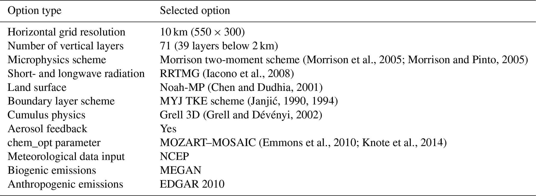
There are several gas-phase chemistry and aerosol treatments available in WRF-Chem v4.2.2. In the current study, the Model of Ozone and Related chemical Tracers version 4 (MOZART v4) gas-phase mechanism (Emmons et al., 2010; Knote et al., 2014) is used in combination with the Model for Simulating Aerosol Interactions and Chemistry (MOSAIC) four-bin aerosol scheme (Zaveri et al., 2008). Four size bins (0.039–0.156, 0.156–0.625, 0.625–2.500, and 2.5–10.0 µm dry diameters) are used in the MOSAIC aerosol module for the representation of the aerosol size distribution. The PBL scheme used in our simulation is the Mellor–Yamada–Janjić (MYJ) turbulent kinetic energy (TKE) scheme (Janjić, 1990, 1994), and the land surface model scheme is the Noah land surface model scheme (Chen and Dudhia, 2001). The cumulus scheme is the Grell 3D cumulus scheme (Grell and Dévényi, 2002), which performs better than other schemes (Hasan and Islam, 2018). The cloud microphysics scheme is the Morrison two-moment microphysics scheme (Morrison et al., 2005; Morrison and Pinto, 2005). Model radiation treatment utilizes the Rapid Radiative Transfer Model for GCMs (general circulation models) (RRTMG) shortwave and longwave radiation schemes (Iacono et al., 2008), including the aerosol radiation feedback.

Meteorological initial and lateral boundary conditions for WRF-Chem simulation were obtained from the National Centers for Environmental Prediction (NCEP) Global Data Assimilation System (GDAS) Final (FNL) analysis at 0.25° spatial resolution and 3 h temporal resolution. The initial and lateral conditions of chemical species are obtained from the Whole Atmosphere Community Climate Model (WACCM) at 0.9°×1.25° resolution with 88 levels. Key species associated with wildfires are included: carbon monoxide (CO), carbon dioxide (CO₂), black carbon (BC), nitrous oxide (N₂O), nitrogen oxides (NO_x), and so on (Mills et al., 2016). In addition, the Fire Inventory from NCAR (National Center for Atmospheric Research) version 2.4 (FINNv2.4) is used as fire emission input for the simulation. The model simulation was conducted over two nested domains: an outer domain covering the Canadian region (25–67° N and 70–140° W) and an inner domain focused on the CONUS region (25–50° N and 64–125° W). The simulation spanned 9–25 August 2018, with a spatial resolution of 10 km for the inner domain and 71 vertical layers from the surface to the top of the atmosphere (TOA). More details of the model configurations are shown in Table 1.

(Morrison et al., 2005; Morrison and Pinto, 2005)(Iacono et al., 2008)(Chen and Dudhia, 2001)(Janjić, 1990, 1994)(Grell and Dévényi, 2002)(Emmons et al., 2010; Knote et al., 2014)

Table 1 Parameterizations used in WRF-Chem model simulations. Noah-MP: Noah-Multiparameterization, MEGAN: Model of Emissions of Gases and Aerosols from Nature.

4 Methods

This section mainly describes the methods we used to estimate pollution changes in the continental US due to long-range transported smoke. We first describe the method we used for filling the AOD gaps of the MAIAC satellite AOD product and then describe two different methods for estimating surface PM_2.5. Finally, we discuss how we assess the surface pollution change due to Canadian wildfires.

4.1 Filling the AOD gaps

To reiterate, one of the goals of the study is to estimate daily surface PM_2.5 at 0.1° spatial resolution. AOD alone cannot provide necessary spatial coverage due to gaps in cloud cover. Therefore, we explored two commonly used methods for filling the AOD gaps. One commonly used method for daily AOD gap-filling problems is Kriging interpolation (Kianian et al., 2021; Singh et al., 2017). At the same time, the performance of Kriging interpolation degrades with increasing distances from the training points, which implies a limitation of the method in large areas of missing data (Kianian et al., 2021). Therefore, in the second method, we combine the Kriging method with outcomes from our CTM simulations to improve the AOD gap interpolation.

4.1.1 Kriging interpolation

The ordinary Kriging (OK) method computes the estimation of an unsampled point based on the weighted average of surrounding pixels (Zandi et al., 2011). Several authors have fully described the theoretical basis of this method (Cressie, 1988; Emery, 2005), and it has proven to successfully fill in the AOD gaps for air pollution studies (Ma et al., 2014). The estimated AOD value at an unsampled location (×0) can be expressed as

$$\begin{array}{}\text{(2)}& {\displaystyle }{\displaystyle }{Z}^{\prime }\left(x_{\mathrm{0}}\right)=\sum _{i=\mathrm{1}}^n{\mathit{\lambda }}_{i}Z\left(x_i\right),\end{array}$$

where i=1, 2, 3, …, n represent for the surrounding pixels and λ_i is the Kriging weight. A major factor that expresses the spatial dependence between neighboring points is the variogram (Arslan, 2012), which is defined as

$$\begin{array}{}\text{(3)}& {\displaystyle }{\displaystyle }{\mathit{\gamma }}_h={\displaystyle \frac{\mathrm{1}}{\mathrm{2}n}}\sum _{i=\mathrm{1}}^n\left[Z\right(x_i)-Z(x_i+h){]}^{\mathrm{2}},\end{array}$$

where Z(x_i) is the AOD value at point i and Z(x_i+h) is the AOD value of other points that have a discrete distance h from point i. Previous studies have applied the OK method with an exponential variogram (or semi-variogram) of interpolating missing AOD values (Lv et al., 2016; Hu et al., 2019). Therefore, in this study, we use the OK method with an exponential variogram to obtain first-stage gap-filling daily AOD over our study area.

4.1.2 CTM interpolation

We applied the Kriging method for interpolation in areas with sufficient AOD information while using CTM interpolation where valid AOD retrievals were unavailable to minimize uncertainties associated with small-scale “missingness” of AOD. These uncertainties arise because CTM relies on fire inventories derived from satellite fire detection products, which may fail to capture small-scale fires due to the spatial resolution of satellite observations and fractional fire coverage within a pixel (Fu et al., 2020). Such undetected fire sources can lead to inaccuracies in CTM outputs. To better represent the AOD distribution in regions with small-scale missingness, we prioritize the Kriging method over CTM interpolation. Therefore, our gap-filling method accepts Kriging interpolation in regions with a small missing portion (<20 %). At the same time, we feed the interpolation with CTM outputs for regions with a more significant missing portion. The details of the process are shown in Fig. 1.

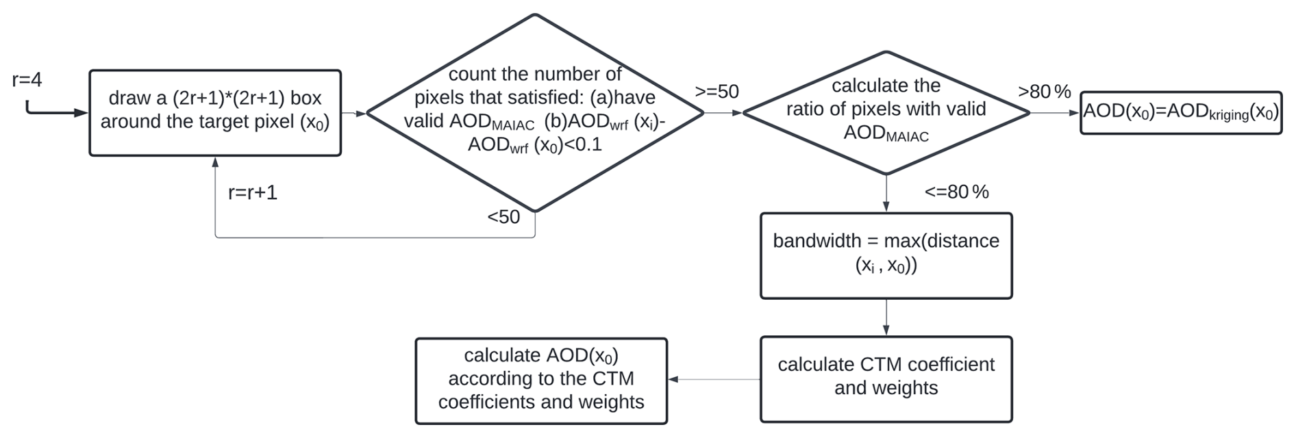
Figure 1 Flowchart of the AOD gap-filling process. r refers to the radius of the selected box used in the process.

To estimate the AOD value for a location without valid MAIAC AOD data, we first select a 9 pixel×9 pixel box (spatial resolution of 0.1°) centered on the target pixel. Within this box, we identify pixels that satisfy two conditions: (a) having valid MAIAC AOD data and (b) having a small AOD_wrf difference (<0.1) compared to the target pixel. If fewer than 50 pixels meet these criteria, the box radius is expanded and the filtering process is repeated. Once at least 50 pixels are identified, we calculate the ratio of valid MAIAC AOD pixels to the total number of pixels in the box, where total pixels refer to all pixels in the selected box, regardless of filtering. If the ratio exceeds 80 %, the AOD for the target pixel is estimated using the ordinary Kriging (OK) method, based on the filtered pixels. However, if the ratio is 80 % or lower, the AOD is calculated using a geographically weighted regression method that considers the neighboring ratio between MAIAC AOD and AOD_wrf:

$$\begin{array}{}\text{(4)}& {\displaystyle }{\displaystyle }\text{AOD}\left(x_{\mathrm{0}}\right)={\text{AOD}}_{\text{wrf}}\left(x_{\mathrm{0}}\right)\cdot R,\end{array}$$

where R is the weighted ratio which can be expressed as

$$\begin{array}{}\text{(5)}& {\displaystyle }& {\displaystyle }R=\sum _{i=\mathrm{1}}^n(\mathit{\alpha }\cdot w),\text{(6)}& {\displaystyle }& {\displaystyle }\mathit{\alpha }={\displaystyle \frac{{\text{AOD}}_{\text{MAIAC}}\left(x_i\right)}{{\text{AOD}}_{\text{wrf}}\left(x_i\right)}},\text{(7)}& {\displaystyle }& {\displaystyle }w={\displaystyle \frac{\mathrm{1}-\frac{\text{distance}(x_i,x_{\mathrm{0}})}{\text{bandwidth}}}{{\sum }_{i=\mathrm{1}}^n\left(\mathrm{1}-\frac{\text{distance}(x_i,x_{\mathrm{0}})}{\text{bandwidth}}\right)}},\end{array}$$

where distance(x_i,x₀) means the distance between location x_i and x₀ and the bandwidth is selected based on the maximum distances between point x_i with valid MAIAC AOD data and target pixel x₀ within the preselected box. According to the above equations, we can obtain the AOD prediction for the unsampled location x₀.

4.2 Estimating surface PM_2.5 using the gap-filled AOD

Having the gap-filled AOD data, we can now estimate the surface PM_2.5 with more extensive spatial coverage. In this study, we tested two methods (GWR and RF, random forest) for predicting surface PM_2.5 using the gap-filled AOD with other meteorological variables. Due to characteristics of the regional wildfires, we chose both methods to consider spatial variations in pollution distribution. After comparing the fitting and validation results of the two methods, we apply the method with the better performance to estimate daily surface PM_2.5.

Before we perform the prediction, different datasets need to be resampled to the exact grid resolution. Grids with 0.1° spatial resolution are constructed over the study region. For AOD data with 1 km resolution, we average all valid AOD values that fall into the same grid. Moreover, for other meteorological variables with a 0.25° resolution, we apply the inverse distance method to scale up all the variables into the predefined grids. PM_2.5 measurements in the same grid are averaged to one value to obtain a 0.1° resolution. In order to derive the relation between PM_2.5 and AOD, we select data where AOD and surface PM_2.5 are both available (AOD>0 AND ${\mathrm{PM}}_{\mathrm{2.5}}>\mathrm{2.0}\mathrm{\mu }\mathrm{g}{\mathrm{m}}^{-\mathrm{3}}$) to train the models.

4.2.1 GWR method

To derive the surface PM_2.5 using filled AOD with other meteorological variables, we used a GWR model that we fully describe in our prior work (Xue et al., 2021). The GWR model has advantages over other methods because it estimates spatially varying relationships. The disadvantage of GWR model, on the other hand, is that the coefficients change daily according to different spatial characteristics of surface pollution, indicating increased computational expenses. To account for varying degrees of freedom centered on different locations, adaptive bandwidth, selected by the Akaike information criterion (AIC), is used for the GWR model. The model can be described as

$$\begin{array}{ll}{\displaystyle }{\mathrm{PM}}_{\mathrm{2.5},i,t}=& {\displaystyle }{\mathit{\beta }}_{\mathrm{0},i,t}+{\mathit{\beta }}_{\mathrm{1},i,t}{\text{AOD}}_{i,t}+{\mathit{\beta }}_{\mathrm{2},i,t}{\text{BLH}}_{i,t}\\ {\displaystyle }& {\displaystyle }+{\mathit{\beta }}_{\mathrm{3},i,t}{\text{T2M}}_{i,t}+{\mathit{\beta }}_{\mathrm{4},i,t}{\text{U10M}}_{i,t}\\ \text{(8)}& {\displaystyle }& {\displaystyle }+{\mathit{\beta }}_{\mathrm{5},i,t}{\text{RH}}_{i,t}+{\mathit{\beta }}_{\mathrm{6},i,t}{\text{SP}}_{i,t}+{\mathit{ϵ}}_i,t,\end{array}$$

where i represents different locations, t represents different days, and β stands for the weight coefficients for different variables. The value of β depends on the geographical weighting of surrounding observations within the bandwidth. The weighting of each observation point decreases according to an exponential curve as the distances from the target point increase.

To test the GWR model, we must preserve only a small portion of the data, leaving most data to train the model since GWR requires an adequate number of samples, and the distribution of ground observations is uneven across the nation. Leave-one-out cross-validation (LOOCV) can be a relatively accurate way to test the model, but it comes at a high computational cost (Xue et al., 2021). Additionally, k-fold cross-validation with large fold numbers shows similar results (Xue et al., 2021). Therefore, we performed 100-fold cross-validation to evaluate the model performances. The inputs for the model are split into 100 subsets, and each time, we use one subset as testing samples, while the other 99 subsets are used as fitting samples, after repeating this process 100 times until we test the whole dataset. Finally, we evaluate the model performance by comparing the correlation coefficient (R) and root mean squared error (RMSE) of model fitting and cross-validation.

4.2.2 Random forest method

Random forest is a non-parametric model that conducts estimations of prediction values by constructing a large number of decision trees. RF randomly divides nodes into sub-nodes for each tree, and the average estimation of different trees makes up the final results (Jiang et al., 2021a; Breiman, 1996). Of various machine learning methods, RF usually outperforms other machine learning methods due to its simplicity, diverse applications, and tackling of complex cross-sensitivities, among various features (Gupta et al., 2021; Jiang et al., 2021a; Zimmerman et al., 2018). The two vital parameters that affect the model performance are the tree number in the forest and feature numbers. We use 100 trees and 6 features in this study.

For our study period, a total of 11 942 samples are collected for training the model. The number of variables is the same as the inputs for the GWR model in order to maintain consistency (AOD, BLH, T2M, U10M, RH, SP, latitude, longitude, and day number). We also performed the same cross-validation as the GWR model to test the model performance so that the prediction accuracy can be compared between the two models. The model that performs better is selected to estimate the surface PM_2.5 for locations where no PM_2.5 observations are available based on (a) the results of the cross-validation and (b) the differences in results (RMSE and correlation coefficients R) between model fitting and validation. Note that a lower RMSE and higher R indicate high prediction accuracy, and a slight difference in model fitting and validation means the model is not overfitting.

4.3 Assessing the pollution increase caused by Canadian fires

The model that performs better from the previous step is used for estimating the gaps in surface PM_2.5. To further assess the surface pollution change due to long-range transported smoke from Canadian wildfires, we conduct a control run of WRF-Chem with all fire emissions within Canada turned off, while emissions in the US are kept the same. The simulated surface PM_2.5 of the control run (hereafter PM_2.5,control) and Canadian fire run (experiment run, PM_{2.5,experiment}) is then converted to surface PM_2.5 based on the relation derived from previous steps:

$$\begin{array}{}\text{(9)}& {\displaystyle }{\displaystyle }{\mathrm{PM}}_{\mathrm{2.5},\mathrm{control}}={\mathrm{PM}}_{\mathrm{2.5}}\cdot {\displaystyle \frac{{\mathrm{PM}}_{\mathrm{2.5},\mathrm{WRF},\mathrm{control}}}{{\mathrm{PM}}_{\mathrm{2.5},\mathrm{WRF},\mathrm{experiment}}}},\end{array}$$

where PM_2.5 is the estimated PM_2.5 concentration using the model that performed better (GWR or RF). The differences between PM_2.5,control and PM_2.5 are then calculated to quantify the pollution change due to long-range transported smoke.

5 Results

5.1 Smoke plumes from Canadian wildfires transport to the US

Figure 2 shows the AOD change due to Canadian wildfires from 17–20 August 2018. The changes in AOD distribution with and without Canadian fires vary according to wind directions and fire sources. The AOD change during the study period varies between 0 and 2.2 based on the two WRF-Chem simulations. The change is most prominent in North Dakota and Minnesota on 17 August, and the Canadian smoke continued to move southward to Iowa on 18 August. In the meantime, a large amount of Canadian smoke increased (high AOD increase) in northwestern US (including Washington and Montana). On 19 August, Canadian smoke over the northwestern US was transported eastward and more smoke was brought to the central US. On 20 August, Canadian smoke moved further to southern regions, due to a storm system, while the AOD values decreased, due to precipitation.

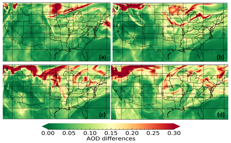
Figure 2 AOD change due to Canadian wildfires from 17–20 August 2018: (a) 17 August 2018, (b) 18 August 2018, (c) 19 August 2018, and (d) 20 August 2018. The AOD change is calculated using the difference of two WRF-Chem simulations.

Canadian wildfire smoke has been consistently identified as a contributor to AOD increases across the US during wildfire seasons. For example, during a 2015 Canadian wildfire event, AOD increases exceeding 1 were observed along the eastern US coast (Yang et al., 2022). In a 2016 event, aerosol height data revealed that Canadian smoke contributed 40 %–60 % of the total column AOD in New York (Wu et al., 2018). Observed AOD increases for high-altitude aerosols from Canadian fires ranged from 0.18 to 0.45 at 532 nm in New York during this period. These findings align with the AOD increases simulated in our study and underscore the significant role of long-range transported Canadian smoke in contributing to regional pollution during wildfire episodes.

5.2 Associations of smoke transport with synoptic-scale pressure patterns

Prior studies show that the transport of smoke aerosols is usually affected by synoptic pressure patterns. High surface pressure often indicates the accumulation of surface pollution, while successive low pressure can also increase surface pollution (Chen et al., 2008). In order to investigate the relationship between synoptic pressure patterns and the smoke transport process, we compared the horizontal and vertical distribution of Canadian smoke in the US.

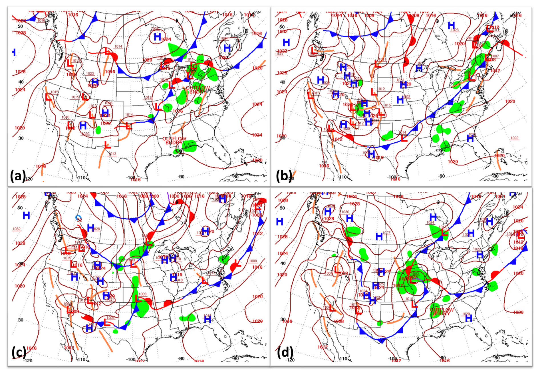
Figure 3 Surface weather maps from 17–20 August 2018 (https://www.wpc.ncep.noaa.gov/archives/web_pages/sfc/sfc_archive.php, last access: 24 May 2025): (a) 17 August 2018, (b) 18 August 2018, (c) 19 August 2018, and (d) 20 August 2018.

According to the surface pressure map on 17 August 2018 (as shown in Fig. 3a), there was a high-pressure system located in Ontario, and its influence extended into parts of North Dakota. This high-pressure system was moving eastward, and as it moved east, the descending air associated with the high-pressure system inhibited vertical convection, leading to the entrapment of smoke in the lower atmosphere. Consequently, the smoke experienced dry deposition at lower altitudes, which explains the low AOD concentration over northeastern Minnesota in Fig. 2a. Smoke at higher altitudes tended to be redirected around the high-pressure system. Simultaneously, there was a low-pressure system situated in the northern Wisconsin region, causing the smoke to move in a northeasterly direction towards this low-pressure area. On 18 August, as shown in Fig. 3b, the high-pressure system shifted to Quebec, and its peripheral influence extended to the Madison region. The presence of this high-pressure system resulted in the formation of a narrow corridor of low AOD distribution within the path of smoke transport, as illustrated in Fig. 2b. On the same day, a low-pressure system was forming over South Dakota and Nebraska. The ascending air and the robust winds along the trough axis established more conducive circumstances for the transportation of Canadian smoke. This phenomenon is clearly illustrated in Fig. 2c, where the smoke expanded further to the south, strongly influenced by the presence of the evolving low-pressure system. By 20 August, this system had transitioned eastward, enveloping the states of Iowa and Missouri, as in Fig. 3d. Intense rainfall and thunderstorms materialized as the low-pressure system rotated over the area. This precipitation served as a scavenging mechanism, effectively eliminating the smoke through a wet-deposition process. Some portions of the smoke, however, carried by the powerful winds, could potentially impact air quality in the southern regions.

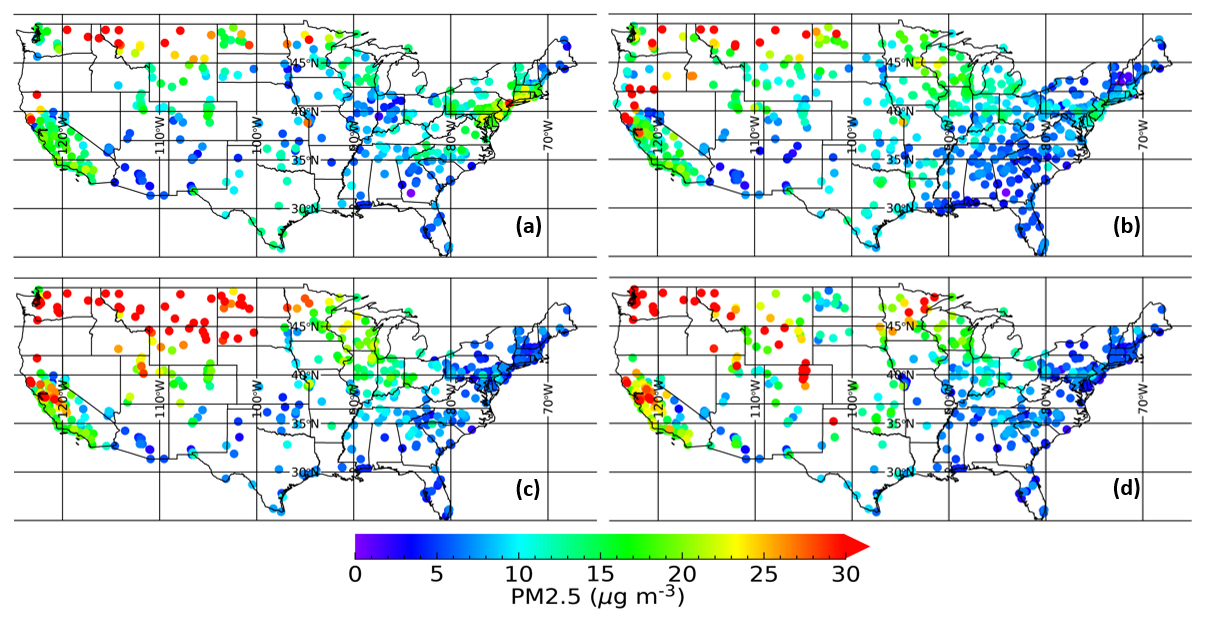
Figure 4 Surface PM_2.5 measurements from EPA stations over CONUS from 17–20 August 2018: (a) 17 August 2018, (b) 18 August 2018, (c) 19 August 2018, and (d) 20 August 2018.

Figure 4 shows the surface PM_2.5 distribution from EPA stations during the 4 d, while Fig. 5 presents the surface PM_2.5 dry mass contributed solely by Canadian wildfires, as derived from the difference between the Canadian fire case and the control case in WRF-Chem simulations. Comparing these figures helps distinguish the contributions of local sources and long-range transported Canadian wildfire smoke to surface pollution in the US. If regions of high PM_2.5 in Fig. 4 correspond to low values in Fig. 5, it suggests that pollution in those areas is predominantly caused by local sources. Conversely, if high values in Fig. 4 align with elevated values in Fig. 5, it indicates that Canadian wildfire smoke is a significant contributor. On 17 August, elevated surface PM_2.5 levels (>10 µg m⁻³) were observed in northern US states. However, in the difference map, areas such as Montana, North Dakota, and South Dakota exhibit low values close to zero, indicating that surface pollution in the northwestern US primarily originated from local fires. On 18 August, a high-pressure system positioned over Minnesota resulted in higher surface PM_2.5 concentrations in that region. However, the difference map shows low values over the same area, indicating that the elevated pollution levels were primarily due to local sources. High-pressure systems typically feature calm winds and stable atmospheric conditions, which trap pollutants near the surface and hinder the transport of Canadian wildfire smoke into the region. By 19 August (Fig. 4c), surface PM_2.5 levels increased across central US states, with high AOD concentrations noted over Utah and Illinois, likely influenced by high-pressure systems. In contrast, elevated PM_2.5 levels in Iowa and Missouri appear to align with the transport of Canadian wildfire smoke. A low-pressure system extending southward facilitated the movement of smoke, reaching as far south as Missouri, thereby expanding the range of smoke transport compared to the preceding days. The impact of the low-pressure system became more pronounced on 20 August (Fig. 4d). In the center of the cyclone, particularly in Iowa and Missouri, wet-deposition processes dominated. The robust winds associated with the low-pressure system carried Canadian smoke, which was subsequently removed by precipitation, leading to no significant increase in surface pollution in these areas. However, along the outer boundaries of the cyclone, from Colorado through Kansas and Oklahoma to northern Texas, surface pollution levels noticeably increased. This increase can be attributed to Canadian smoke transported by the strong winds of the low-pressure system, resulting in heightened PM_2.5 concentrations in these regions.

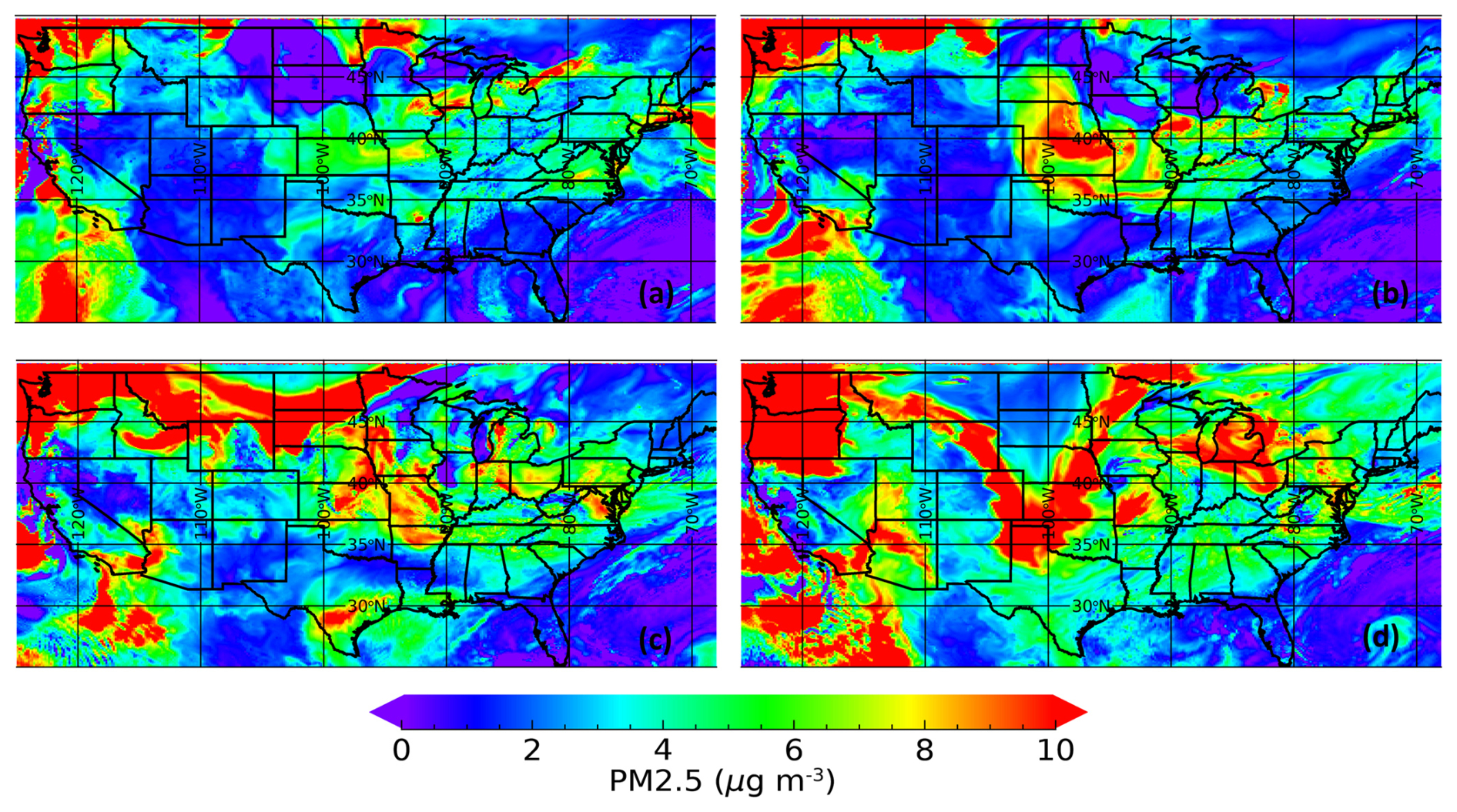
Figure 5 Surface PM_2.5 dry mass difference from WRF-Chem simulations over CONUS from 17–20 August 2018: (a) 17 August 2018, (b) 18 August 2018, (c) 19 August 2018, and (d) 20 August 2018. The PM_2.5 difference is calculated using the two WRF-Chem simulations.

With low-pressure systems in the central US, both model outputs and surface observations show longer southward transport paths of Canadian smoke in the US. Take 20 August as an example; airflows of the extratropical cyclone in Iowa substantially determine the transport direction of the Canadian smoke. To investigate smoke's horizontal and vertical transport, we take the pollution distribution map of three atmospheric layers (773, 850, and 900 hPa) to compare the moving directions of smoke (Fig. 6). In upper layers (773 hPa), Canadian smoke intrudes into the US from two directions: the northwestern US and northeastern US. These two smoke plumes meet in the central US at a higher level and then split in two directions while transporting downward (as shown in the black circles in the 900 hPa map). The downward transport directions can be explained using a conceptual model of the extratropical cyclone (Fig. 6d). Canadian smoke follows the downward airflow: part of the smoke moves southwesterly away from the cyclone, while the rest of the pollution moves toward the cyclone and goes through wet-deposition processes.

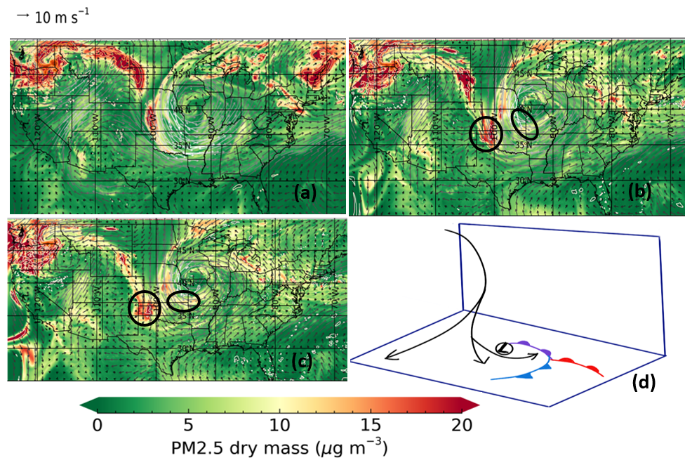
Figure 6 PM_2.5 dry mass distribution on 20 August 2018 at different levels: (a) 773, (b) 850, and (c) 900 hPa. (d) Conceptual model of airflow patterns in a typical extratropical cyclone based on Cotton et al. (2011).

Overall, the horizontal distribution and transport of Canadian smoke are closely related to pressure systems. Surface high pressure usually facilitates the subsidence of elevated Canadian smoke pollution (with surface PM_2.5 increase). In contrast, a low-pressure system tends to have the opposite effect (lifting), corresponding to longer transport distances.

5.3 Daily coverage of satellite AOD and simulated AOD from WRF-Chem

During the wildfire period selected in this study (17 d), we calculate the daily MAIAC AOD coverage using the number of pixels with valid AOD values divided by the total number of pixels. The AOD coverage after combining Aqua and Terra data ranges from 46 % to 68 % (shown in Fig. 7). Analyzing daily AOD coverage is essential, as satellite-derived AOD serves as a columnar indicator of pollution with extensive spatial coverage and high-resolution data, making it a valuable predictor for estimating surface PM_2.5 concentrations alongside other variables. However, it often has missing values over fire-intense regions, which can significantly impact the accuracy of predicted surface PM values. Using model-simulated AOD in conjunction with satellite AOD can help mitigate this issue and improve predictions.

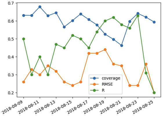
Figure 7 Time series of MAIAC AOD coverage (blue line), with the correlation coefficient (green line) and RMSE (orange line) of two AOD products (WRF-CHEM AOD and MAIAC AOD).

In order to show the spatial distribution of AOD coverage, we also calculate the coverage ratio of AOD of each pixel over the 17 d (shown in Fig. 8). The average AOD coverage for the whole study area is around 60 %. For the northeastern US, 40 %–70 % of the days are covered by clouds, while more than 80 % of the days have valid AOD values in the western US.

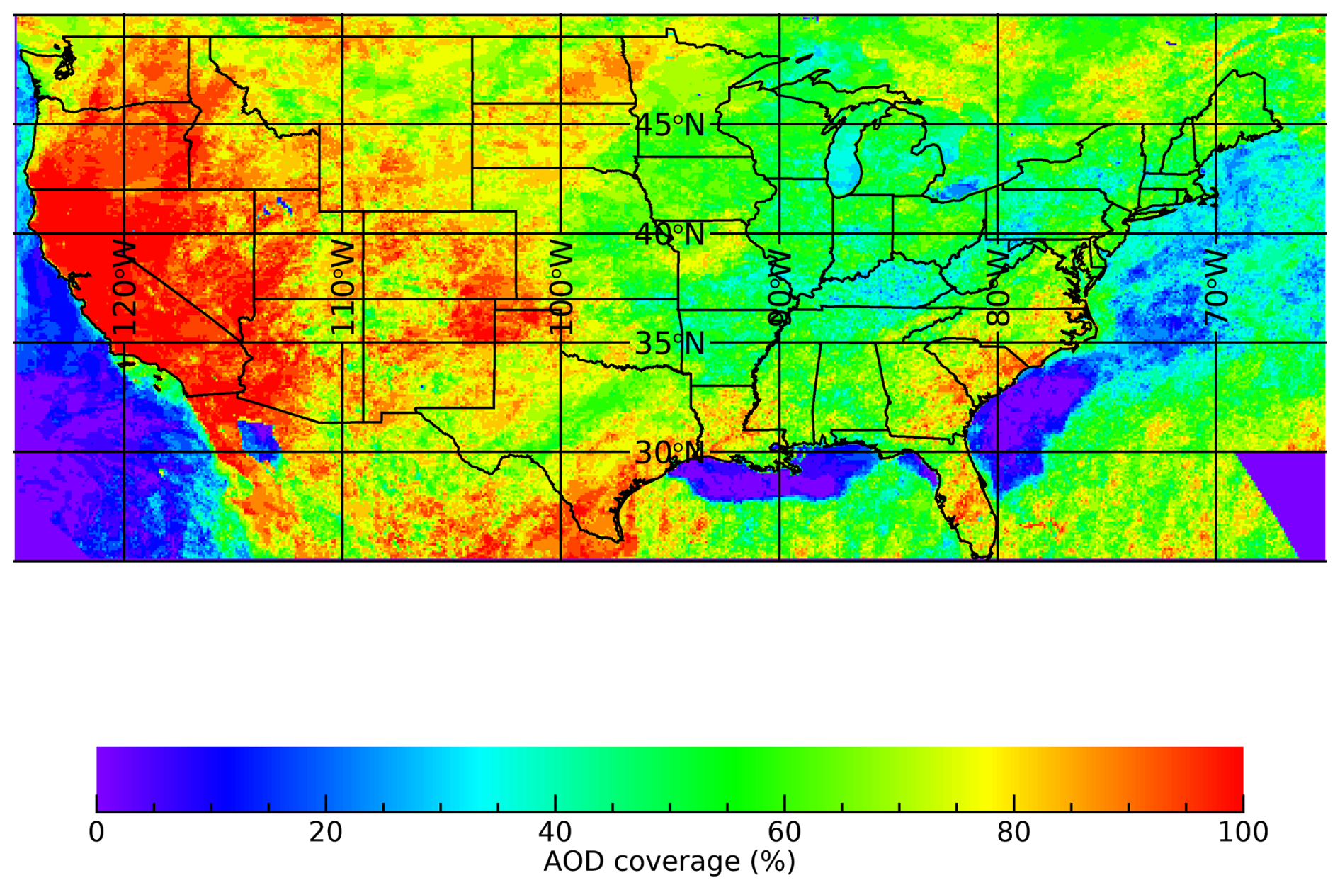
Figure 8 AOD coverage during the 17 d period.

The model-simulated 550 nm AOD has a distribution very similar to the satellite AOD. Comparing MAIAC AOD with corresponding simulated AOD pixels, the correlation coefficients range from 0.3 to 0.63 and the RMSE is within the range of 0.2–0.4 (shown in Table S2 in the Supplement). Time series of the coverage and statistics are shown in Fig. 7. There is no clear correlation between MAIAC AOD coverage and the correlation of two AOD products, as the missing AOD areas for each day are randomly distributed and affected by satellite swath coverage and cloud contaminations. Overall, simulated AOD is lower than satellite AOD potentially due to the underestimation of fire emissions, especially for small-scale fires (Wiedinmyer et al., 2011). FINNv2.4 identified fire sources based on the combinations of the thermal-anomaly product of MODIS and VIIRS (Visible Infrared Imaging Radiometer Suite) (Wiedinmyer et al., 2011; Li et al., 2021). Adding high-spatial-resolution fire detection information from VIIRS increases the total burned area by 280 % compared to the previous FINN version that used MODIS detection only (Li et al., 2021). However, thick smoke and cloud cover primarily affect the detection of fires (Fu et al., 2020; Schroeder et al., 2014), causing AOD underestimation in regions with missing fire detection.

The comparison between WRF-simulated AOD and satellite-retrieved AOD shows a high spatial correlation, indicating a similar smoke pathway between the model and satellite observations. We also compare the ground AERONET AOD with the model-simulated values. The correlation coefficient during the 17 d between the two AOD products is 0.54, and the RMSE is around 0.06. Similar to the comparison with satellite AOD, model-simulated AOD values show underestimations compared to AERONET AOD.

5.4 AOD gap filling

Our gap-filled AOD increased the mean coverage from 60 % to 92 %, and missing values of the gap-filled AOD were mainly distributed at the edges of our study area due to limited satellite retrieval for deriving accurate AOD_filled–AOD_MAIAC relationships.

To illustrate the importance and differences in feeding the interpolation with CTM outputs, we choose 13 August to display the differences when fires are detected near cloud edges. Figure 9 shows the AOD distribution of the CTM-filled AOD, Kriging-filled AOD, and MAIAC AOD. The south-central US region (including Texas, Oklahoma, and Nebraska) has large missing AOD areas due to clouds. The Kriging-filled AOD for this region is evenly distributed with values around 0.3. However, the CTM-filled AOD shows more variations and a clear smoke transport path along the wind direction. The primary reason for this difference is some small-scale fires detected near the cloud edges in Oklahoma. According to the fire emission document (https://www.acom.ucar.edu/Data/fire/data/finn2/README_FINNv2.5_Feb2022.pdf, last access: 24 May 2025), both 375 m resolution VIIRS fire detection and 1 km resolution MODIS thermal anomalies are used for estimating fire emissions. This enhancement in fire detection provides a more accurate estimation of surface pollution in the presence of clouds. Compared with the surface PM_2.5 distribution of this same day, we find the same distribution pattern as our CTM-filled AOD: high PM_2.5 (>20 µg m⁻³) distributed in central Texas all the way to eastern Oklahoma. Therefore, CTM-filled AOD provides closer patterns as observed in the surface pollution distribution of regions with large cloud covers. Our results indicate the inadequacy of Kriging methods in such cases.

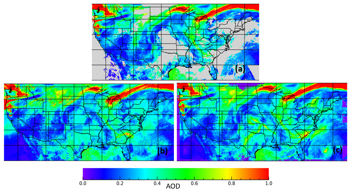
Figure 9 AOD distribution from (a) MAIAC, (b) the Kriging method, and (c) CTM-filled AOD on 13 August 2018.

5.5 Daily PM_2.5 estimation

Figure 10 shows the results of GWR model fitting and cross-validation. The colors represent the probability function that determines the possibility that the ground-level measurements and the estimations from the GWR model are equal to each other. A lighter color means a higher concentration of samples. The R and RMSE of GWR model fitting are 0.85 and 6.2 µg m⁻³, respectively, and the R and RMSE of the 100-fold cross-validation are 0.8 and 7.2 µg m⁻³. The difference between model fitting and cross-validation is relatively small, which means that the model is not overfitting and the prediction accuracy is stable. The slope of the cross-validation best-fit line (solid black line) is 0.72, indicating that the model slightly underestimates the surface PM_2.5, and the biases increase with increasing AOD. The reason for this underestimation is sample biases: (1) a limited number of stations in the western US and (2) EPA stations in the western US are mainly concentrated in the two populated regions, showing extremely uneven distribution. Only 3 % of surface PM_2.5 observations exceeded the unhealthy limit (${\mathrm{PM}}_{\mathrm{2.5}}>\mathrm{35.5}\mathrm{\mu }\mathrm{g}{\mathrm{m}}^{-\mathrm{3}}$) during the 17 d, and among these stations, 62 % of the observations came from stations located in Washington and California. Furthermore, as shown in Fig. 11, the correlation between WRF-Chem-simulated surface PM_2.5 and EPA ground observations is relatively weak (R≈0.4), which underscores the limitations of standalone chemical transport models and further justifies the application of data-driven methods such as GWR.

Figure 10 Fitting and 100-fold cross-validation results for the GWR method (units: µg m⁻³).

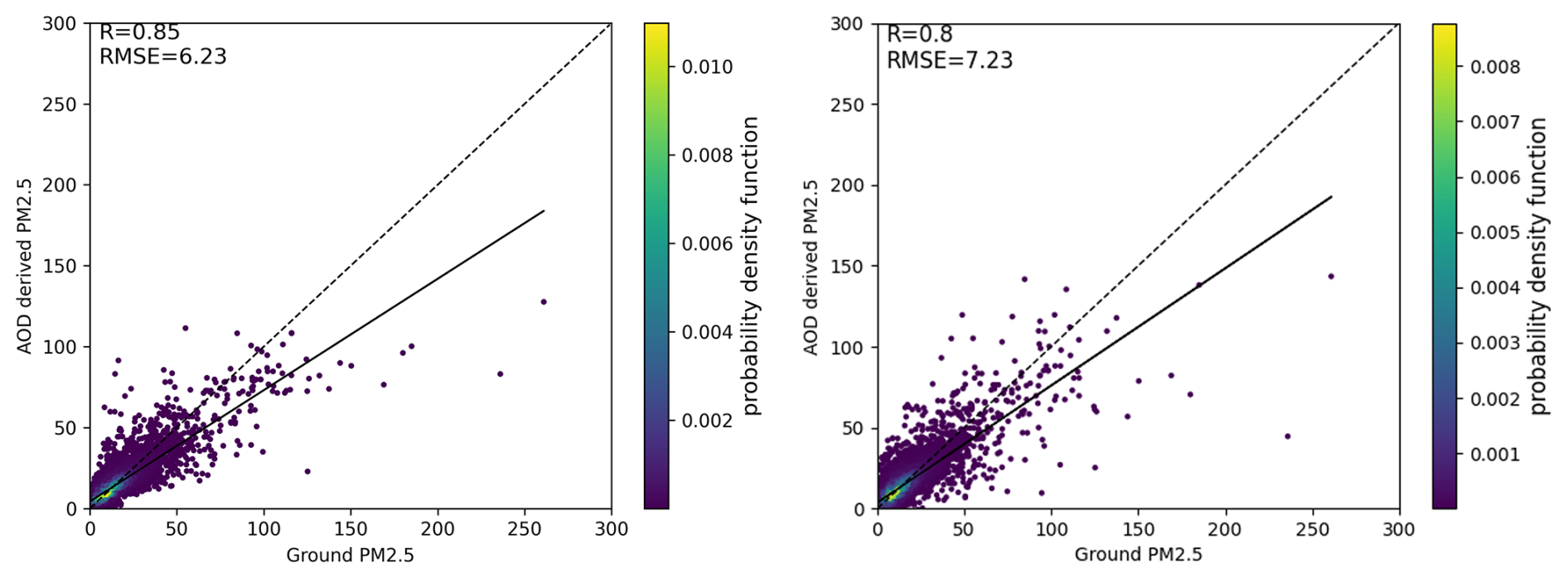
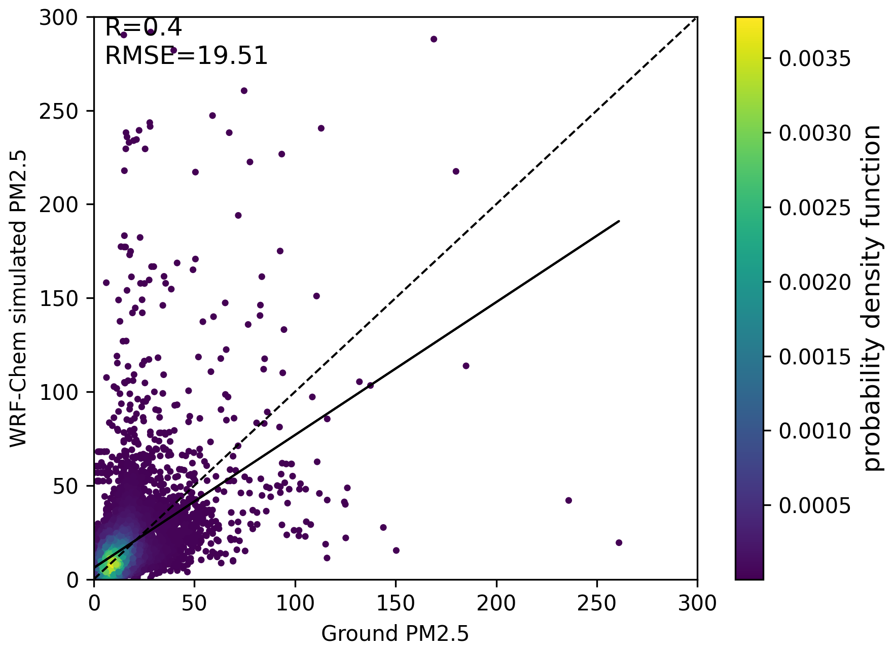
Figure 11 Comparison between WRF-Chem-simulated PM_2.5 and EPA ground-based PM_2.5 measurements (units: µg m⁻³).

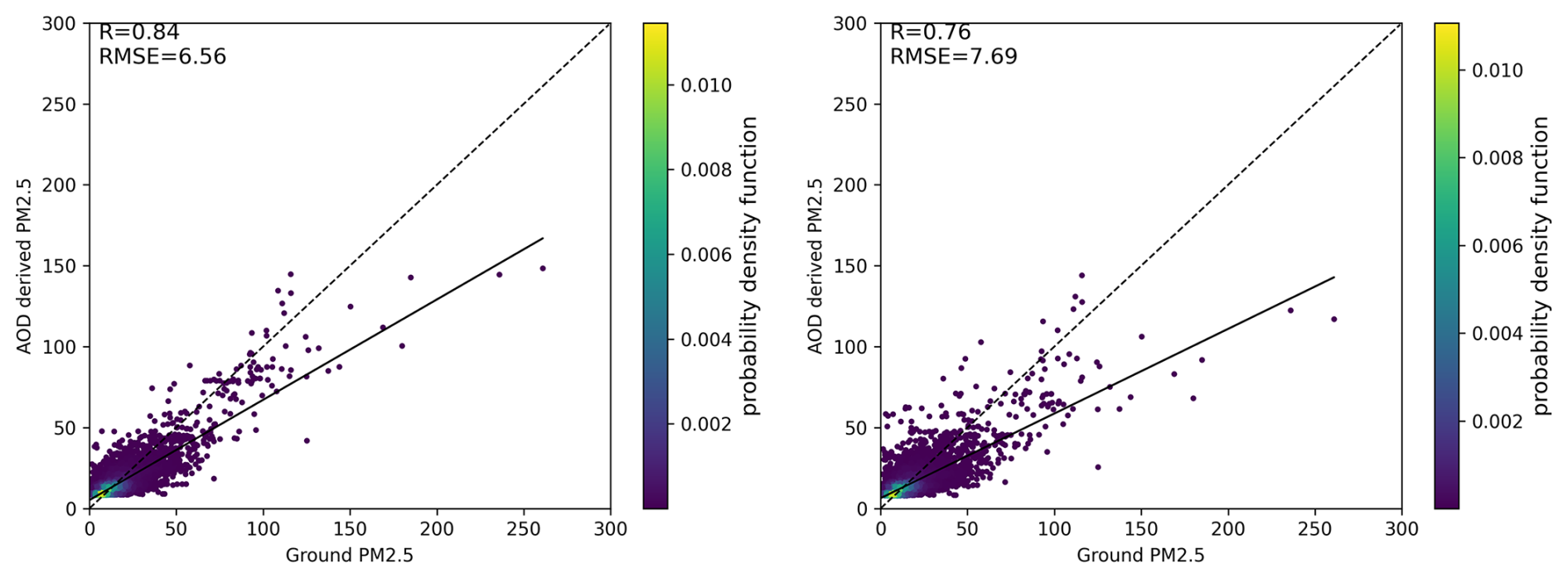
Figure 12 shows the results for RF fitting and cross-validation. The RF model fits well with the training samples with an R of 0.84 and RMSE of 6.56 µg m⁻³, while the cross-validation results degrade significantly (R=0.76, RMSE=7.69 µg m⁻³). The slope of the validation best-fit line is 0.523, which is of lower than that of the GWR method. The difference between model fitting and cross-validation indicates that the model is slightly overfitting and has limited prediction accuracy for this case. One possible reason for this could be the limited number of training samples with average daily available measurements of around 700 during the study period (Jiao et al., 2021). A spatiotemporal RF model can be utilized to enhance RF model performance (Wei et al., 2019). Compared with RF, the GWR model showed slightly higher prediction accuracy and more stability.

Figure 12 Fitting and 100-fold cross-validation results for the RF method (units: µg m⁻³).

Though the difference in cross-validation results for RF and GWR is slight, the daily pollution variation estimated from the two methods shows completely different trends. Figure 13 shows the mean PM_2.5 variation over the three highly polluted areas (EPA Region 8, 9, and 10) during the 17 d period calculated from GWR, RF, and EPA ground stations. For Region 8, EPA stations measured two pollution peaks during the study period: one peak on 19 August and another smaller peak on 24 August. Mean PM_2.5 from the RF method also captured the two peaks on the same day, while the regional mean values were slightly lower than the measurements. However, GWR has a different peak on 11 August but no noticeable increase for the remaining days. For EPA Region 9, both RF and EPA stations show a decreasing trend for the first few days and then slowly increase with time, while GWR has two clear peaks, which are not shown for the other two methods. For the most polluted region, Region 10, the highest peaks from 19 to 22 August are shown in the EPA and RF methods, but GWR shows low values for the same period. The differences between the GWR and RF methods come from the distribution of sample points. In Region 10, most EPA stations are located in Washington, meaning pollution increases there strongly influence the regional mean PM_2.5 when using RF. Conversely, GWR sometimes captures variations in other areas, even when station coverage is sparse. RF is more sensitive to the spatial distribution of ground stations, with its regional mean values closely aligning with EPA station trends. In contrast, GWR is more effective at detecting PM_2.5 variations in areas with limited station coverage. An even distribution of samples could significantly improve estimation accuracy for both methods. Given the observed pollution trends across these highly affected regions, GWR was selected to estimate surface PM_2.5 in this study.

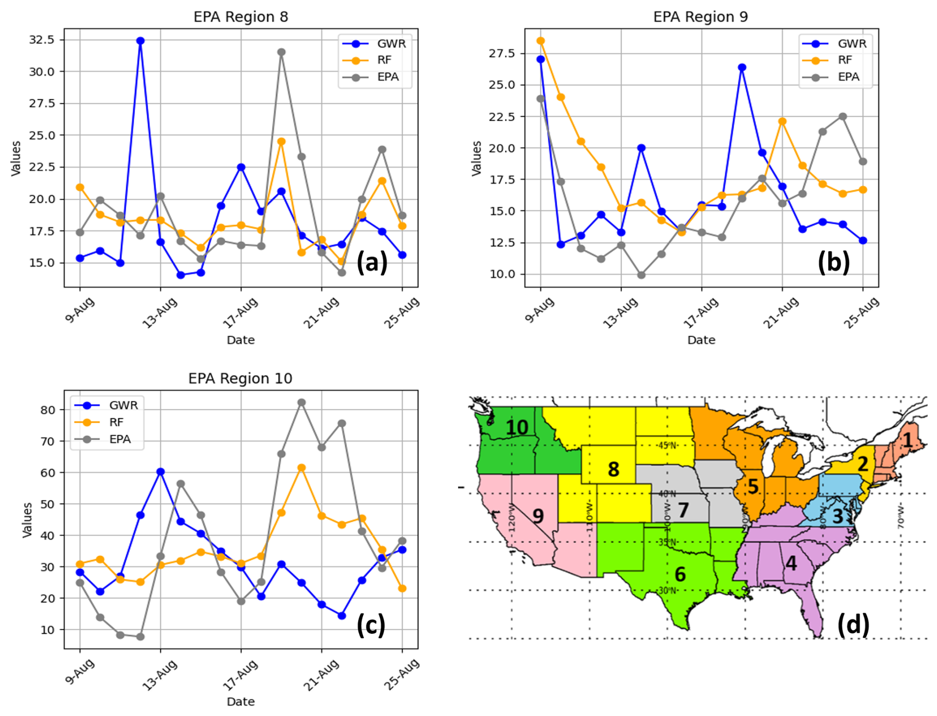
Figure 13 Mean PM_2.5 concentration variations over the top three polluted areas: (a) EPA Region 8, (b) EPA Region 9, and (c) EPA Region 10. (d) EPA region map.

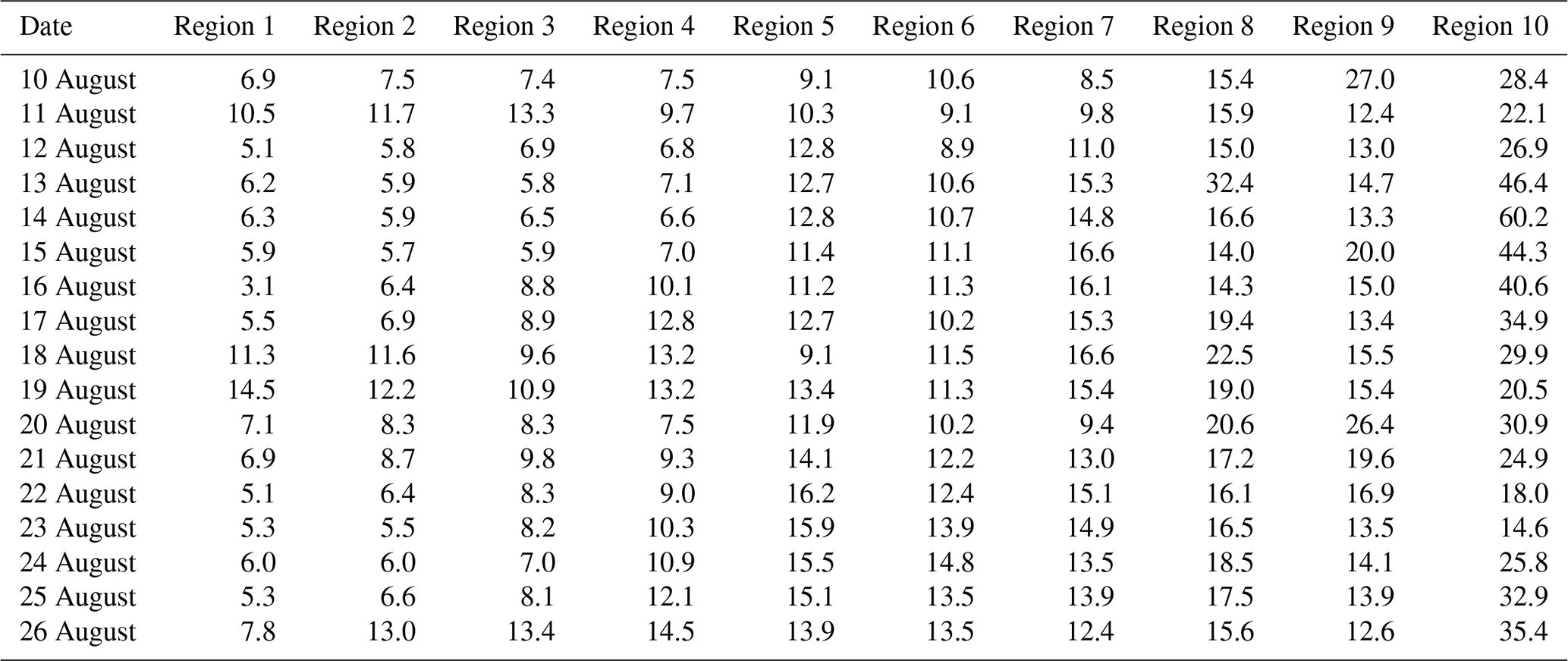
Our GWR daily mean estimation of surface PM_2.5 during the 17 d wildfire event for each EPA region ranges from 3.1 to 60.2 µg m⁻³ (shown in Table 2). The mean surface pollution is highest in Region 10, while it is lowest in Region 1, which is comparable with the previous study (Xue et al., 2021).

Table 2 Mean PM_2.5 concentrations (µg m⁻³) over different EPA regions (1–10) estimated using the GWR method.

5.6 Pollution change due to long-range transported smoke from Canada

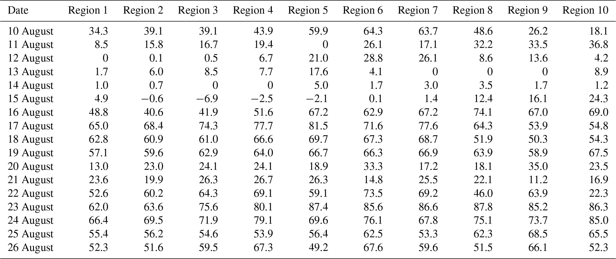
Using coefficients derived from simulated PM_2.5 in control and experiment scenarios, we estimated the PM_2.5 increase attributed to Canadian wildfires. Table 3 presents the daily mean PM_2.5 increase across different EPA regions. The regional mean PM_2.5 increase reached up to 28 µg m⁻³, with Canadian wildfire smoke contributing as much as 87.8 % of total PM_2.5. Region 10 experienced the highest impact, while Region 1 was the least affected. Notably, on some days, the contribution of Canadian wildfire smoke to total PM_2.5 in the northeastern US (Region 1, 2, and 3) exceeded that in the northwestern US (Region 8 and 10). The contribution of wildfire smoke to total PM_2.5 closely followed wildfire activity patterns; however, due to transport distances, it often took time for smoke to travel from Region 10 to Region 1. As a result, during some wildfire episodes, PM_2.5 changes in eastern CONUS lagged behind those in western CONUS by a day.

Table 3 Percentage increase in PM_2.5 concentrations (%) due to Canadian wildfires over different EPA regions (1–10) estimated using the GWR method.

Due to the Clean Air Act (CAA), the overall trend of surface PM_2.5 in the recent years has been one of gradual decrease (Fig. S1 in the Supplement). The decreasing trend is evident in August mean PM_2.5 calculated from EPA surface observations from EPA Region 1 to Region 7, but variations in PM_2.5 in Region 8–10 are more affected by the occurrence of wildfires. For years with low wildfire occurrences (FRP<10 000 MJ), August surface PM_2.5 shows a steady pattern in Region 8 and Region 10 without any apparent rising or dropping. PM_2.5 in Region 9 shows a descending pattern in August in years without large fires, while it can reach up to 3 times more of the baseline in wildfire years. For Region 1–7, August mean PM_2.5 concentrations decrease about 5 %–10 % each year in different regions. Compared with Table S1 in the Supplement, the 17 d investigation highlights how long-range transported smoke from Canada temporarily offsets the descending trend in surface PM_2.5 during the study period. For Region 8–10, wildfires (including contributions from both local and remote fires) increase the August mean surface PM_2.5 by 0 %–98 %. While this study focuses on a short-term event, it demonstrates the significant seasonal impact of Canadian smoke on air quality, emphasizing the need for multi-year investigations to assess long-term trends in Canadian smoke contributions.

In conclusion, due to the concurrent local and remote wildfires, the long-range transport smoke contributed to about half of the surface pollution increase in EPA Region 8, 9, and 10. For other EPA regions, Canadian smoke compensated the CAA, causing surface pollution to rise.

5.7 Uncertainties and limitations

The main uncertainties and limitations of this study come from the CTM model and various inputs of the model, and the surface pollution estimation model also leads to some uncertainties.

1. Since satellite fire detection is affected by various factors, including cloud cover, fire sizes, and the background environment, emission inputs for the WRF-Chem simulations derived from the fire detection products introduce uncertainties into our simulations and create regional biases in the simulated AOD values.

2. In addition to the fire detection biases, assumptions made in computing fire emissions also cause the following uncertainties that affect the simulations: (a) fire sizes and duration, (b) amount and distribution of biomass fuels, and (c) fraction of different emissions from the biomass fuel (Soares et al., 2015). These factors may influence the mass concentration and distribution of smoke aerosols.

3. Uncertainties in the injection height of smoke plumes in WRF-Chem can impact simulation accuracy. Biases in injection height influence horizontal transport speed, direction, and pollution residence time, potentially introducing errors in the AOD gap-filling process. Moreover, uncertainties in the vertical distribution of aerosols can affect the AOD–PM_2.5 relationship, with variations in plume height between monitors leading to inaccuracies in estimated surface PM_2.5 concentrations.

4. The unevenly distributed EPA stations primarily affect the performance of the two PM_2.5 estimation models, causing completely different daily variation trends of regional mean PM_2.5. Therefore, the model performance may be improved if we use more EPA stations (we use FRM monitors only in this study).

5. Since we need the relationships between satellite AOD and CTM AOD to calculate the filled AOD values, the filling values cannot be derived if the area of missing satellite AOD is larger than the radius thresholds we set for deriving the relationships. For days with large areas of missing satellite AOD in the boundary region of our study region, we sometimes have missing AOD values at the boundary. This can be improved by increasing the radius thresholds or the study region to leave space for the boundaries.

6 Conclusions

This study first analyzed the influence of different physical processes on the transport of long-range transported smoke aerosols by comparing two WRF-Chem simulations with and without Canadian wildfires. Then we utilized the simulated AOD from CTM and Kriging interpolation with a geographically weighted method to fill in the daily AOD retrieval gaps caused by cloud cover. Then we estimated the surface PM_2.5 concentration using the GWR and RF methods and tested the two predictions using cross-validation and trend analysis to choose the better-performing method. Finally, by turning off the Canadian wildfire emissions in the CTM simulations, we calculated the surface PM_2.5 concentrations from the CTM AOD outputs using the coefficients derived from previous estimations. The differences in PM_2.5 of the two estimations indicated the change brought by long-range transported smoke from Canadian wildfires. The main findings of our study are the following:

1. Synoptic-scale pressure systems are the dominant drivers of horizontal pollution transport pathways. In the meantime, the pressure systems can also affect the vertical distribution due to ascending or descending smoke. Under most circumstances, the subsidence flow of high-pressure systems facilitates the drifting process of elevated smoke layers and thus increases surface pollution. In contrast, the cyclonic storm system leads to a longer transport path (further south of CONUS in this study) and directs the elevated smoke to the ground in different directions. Therefore, the co-occurrence of low-pressure systems and smoke aerosols corresponds to larger pollution areas.

   Certain weather patterns can facilitate the dispersion of smoke; hence, during severe wildfire events, it becomes crucial to closely monitor the meteorological conditions and alert the public about the potential risks of deteriorating air quality, even if the fires are hundreds of miles away. Furthermore, when conducting prescribed fire burning, it is essential to take into account the possibility of smoke being transported to densely populated areas. In other words, proper consideration of the weather conditions and potential wind patterns is crucial to minimizing the impact on nearby populations.

2. Daily AOD coverage combining the Aqua and Terra MODIS satellites range from 46 % to 68 % during our study period, and our filled AOD values using CTM AOD outputs are able to fill in the missing gaps.

3. Daily PM_2.5 estimations using the filled AOD product with other meteorological data using the GWR method (R=0.8) perform better than the RF model (R=0.76), and the RF model captures the daily variations in different EPA regions calculated from EPA stations.

4. The regional mean increase in surface PM_2.5 concentrations that came from Canadian wildfire smoke ranges up to 28 µg m⁻³ (a 69 % increase), and EPA Region 10 is most affected by Canadian fires, while Region 1 is the least affected. The PM_2.5 change pattern in eastern CONUS often lags behind that in western CONUS by a day.

Our study found that the presence of synoptic-scale pressure systems leads to a higher proportion of the CONUS region being affected by long-range transported smoke from Canada. Typical airflow patterns that are associated with extratropical cyclones are particularly effective at transporting elevated layers of smoke to the surface and fanning the associated particulate pollution over large areas. Such transport pathways associated with extratropical cyclones need to be considered when forecasting the effects of smoke pollution from Canadian wildfires on vulnerable populations in the CONUS region. Our study highlights the significant contribution of wildfires to particulate pollution during the study period, aligning with prior research that suggests wildfires are becoming an increasingly important source of particulate pollution as industrial pollution declines due to stringent regulations (Xue et al., 2021). However, further multi-year investigations are needed to robustly confirm this trend on a broader temporal scale.