High-resolution greenhouse gas flux inversions using a machine learning surrogate model for atmospheric transport

Quantifying greenhouse gas (GHG) emissions is critically important for projecting future climate and assessing the impact of environmental policy. Estimating GHG emissions using atmospheric observations is typically done using source–receptor relationships (i.e., “footprints”). Constructing these footprints can be computationally expensive and is rapidly becoming a computational bottleneck for studying GHG fluxes at high spatio-temporal resolution using dense observations. Here, we demonstrate a computationally efficient GHG flux inversion framework using a machine learning emulator for atmospheric transport (FootNet) as a surrogate for the full-physics model. The footprints generated by FootNet are at approximately 1 km resolution. We update the architecture of the deep-learning model to improve the performance in a GHG flux inversion. We find that the posterior fluxes estimated with FootNet footprints are in good agreement with the posterior fluxes estimated with STILT footprints. We observe that the more simplistic representation of transport in the machine learning model helps to mitigate transport errors. This flux inversion using a machine learning surrogate model requires only meteorological data, GHG measurements, and prior fluxes. Constructing footprints using FootNet is 650 times faster than the full-physics atmospheric transport model on similar hardware. This speedup allows for the computation of footprints “on the fly” during the GHG flux inversion (i.e., computed as needed, rather than archiving for future use) and makes near-real-time emission monitoring computationally possible. This work alleviates a major computational bottleneck with inferring GHG fluxes with next-generation dense observing systems.

1 Introduction

Carbon dioxide (CO₂) and methane are the two most powerful greenhouse gases (GHGs). Together, they account for more than 85 % of the total GHG radiative forcing since preindustrial times (IPCC, 2023). As such, it is important to quantify the GHG sources and sinks in order to project future climate. Near-real-time quantification of GHG emissions is key to identifying the intermittent super-emitters, which often dominate the emission budget. However, the large computational and storage costs associated with full-physics atmospheric transport models in the current inversion framework limit our ability to perform near-real-time emissions monitoring from urban to global scales (Roten et al., 2021; Varon et al., 2023; Cartwright et al., 2023; Fillola et al., 2023; Nayagam et al., 2023; Steiner et al., 2024; Janardanan et al., 2024). Here, we use FootNet (He et al., 2025), a computationally efficient deep-learning model, to emulate a full-physics atmospheric transport model and conduct GHG flux inversions. This work shows the feasibility of using a machine learning (ML) emulator for near-real-time computation of source–receptor relationships and to infer hourly GHG emission fluxes at the kilometer scale from atmospheric observations.

Previous work has shown the importance of point sources for methane emissions (e.g., Brandt et al., 2014; Zavala-Araiza et al., 2015; Frankenberg et al., 2016; Duren et al., 2019; Lauvaux et al., 2022; Chen et al., 2022; Cusworth et al., 2022; Sherwin et al., 2023; He et al., 2024) and urban and localized sources for CO₂ (e.g., Hutyra et al., 2014; Janardanan et al., 2016; Turner et al., 2020; Wu et al., 2020; Kiel et al., 2021). These sources represent a small geographical area and yet dominate the GHG emission budget. The emission fluxes from these “super emitters” are often observed to have a heavy-tailed distribution (Brandt et al., 2014; Zavala-Araiza et al., 2015; Frankenberg et al., 2016; Duren et al., 2019; Chen et al., 2022; Cusworth et al., 2022). In other words, a small number of point sources are responsible for a large fraction of the total emission budget, despite representing a small fraction of the land area. As such, studying these point sources requires densely spaced measurements due to their localized nature. Fortunately, there has been a proliferation of next-generation, dense observing systems for GHGs over the past decade, including both spaceborne instruments, e.g., OCO-2 (O'Dell et al., 2012; Crisp et al., 2012; Eldering et al., 2012; Hammerling et al., 2012), OCO-3 (Eldering et al., 2019; Taylor et al., 2020), and TROPOMI (Veefkind et al., 2012), and low-cost urban monitoring networks (e.g., BEACO₂N: Shusterman et al., 2016).

Measurements from dense observing systems can be used to quantify surface fluxes. The inverse modeling of GHG emissions often requires one to know the upwind region of influence on the atmospheric measurements. This region of influence is also known as the “source–receptor relationship” or the measurement “footprint” (see Rodgers, 2000). The ith observation (y_i) can be related to the m surface fluxes using the associated footprint:

$$\begin{array}{}\text{(1)}& y_i={\mathit{h}}_i\mathit{x}+b_i,\end{array}$$

where h_i is the 1×m footprint for the ith observation, x is an m×1 vector of surface fluxes, and b_i is the background concentration for the observation. Here, h_i describes the sensitivity of observation y_i to m surface fluxes with units similar to $\mathrm{ppm}(\mathrm{\mu }\mathrm{mol}{\mathrm{m}}^{-\mathrm{2}}{\mathrm{s}}^{-\mathrm{1}}{)}^{-\mathrm{1}}$. Similarly, the vector of the n observations (y; n×1) can be related to the surface fluxes as

$$\begin{array}{}\text{(2)}& \mathit{y}=\mathbf{H}\mathit{x}+\mathit{b},\end{array}$$

where b is n×1 vector of background concentrations, and H is an n×m Jacobian matrix representing the atmospheric transport, such that the ith row of H describes the sensitivity of the ith observation (y_i) to the m surface fluxes.

Researchers construct this source–receptor relationship (H) by running a Lagrangian model n times or an Eulerian model m times. The choice of construction of H will depend on the size of both n and m. There are approximately 800 observations and 15 million state vector elements in each inversion run for this study. Therefore, constructing H will require approximately 800 simulations in the Lagrangian framework or around 15 million simulations in the Eulerian framework. The Eulerian models are not grid agnostic, and the corresponding computational expense increases as the spatial resolution increases (Steiner et al., 2024). For example, the Integrated Methane Inversion (IMI) is an Eulerian-based framework focusing on the regional scale but is limited to 25 km at present (Varon et al., 2022). Variational methods such as 4D-Var can be used with large state and observation spaces. However, it requires computing an adjoint, which is a computationally expensive process. Additionally, this process iteratively minimizes the cost function with many forward runs and, as such, can not be parallelized. The computation cost of 4D-Var is independent of the number of observations but can still be very large. It also requires storing many checkpoint files, which can become very large for high spatial resolution and can have high storage costs. Gaussian plume models are known for their simplicity and are often used for point source modeling (Bovensmann et al., 2010; Nassar et al., 2017; Wang et al., 2020). However, these models typically assume favorable conditions such as constant winds and flat topography, which may not always be the case.

Here, we focus on constructing the source–receptor relationship using a full-physics Lagrangian particle dispersion model (LPDM). As such, this requires constructing n footprints, i.e., one footprint for each measurement.

The LPDM can be used to construct a footprint by advecting an ensemble of particles backwards in time from the measurement sites using archived meteorology (e.g., Lin et al., 2003). These Lagrangian trajectories are agnostic to the choice of grid and can be easily mapped to a high spatial resolution. Additionally, for this study, n is small as compared to m, and, therefore, it is computationally efficient to use the Lagrangian method of constructing H.

The computation of footprints from a full-physics LPDM is an embarrassingly parallel problem and, as such, can easily be parallelized. However, this does not overcome the sheer volume of data that would need to be generated for a high-resolution GHG flux inversion. The construction of footprints can quickly become computationally intractable as the number of measurements increases, as is the case with dense observing systems.

In addition to the computational cost of constructing footprints described above, there is a storage cost associated with these footprints that increases with the number of measurements. This can also become burdensome as the number of observations increases. As an example, Turner et al. (2018) examined point sources in the Barnett Shale region in Texas and found that generating 1 week of footprints for hourly measurements made by a geostationary satellite instrument required more than 15 million simulations to construct the footprints and over 4 TB to store them. This region represents less than 1 % of the United States. As such, many previous studies investigating point sources have focused on a subset of cases with favorable atmospheric conditions, allowing them to utilize a simplified representation of atmospheric transport. For example, recent work estimated CO₂ emissions from individual power plants using a Gaussian plume (e.g., Nassar et al., 2017, 2021; Guo et al., 2023), which is only valid for steady winds.

Recent work have explored the potential of machine learning and other analytical methods to address computational bottlenecks when working with LPDMs. For example, Roten et al. (2021) developed an interpolation method using nonlinear weighted averaging to compute footprints. Cartwright et al. (2023) developed a convolution-based variational autoencoder, which predicts footprints using a spatio-temporal Gaussian emulator. Brecht et al. (2023) used neural networks for super-resolution to improve trajectory calculations with the FLEXible PARTicle dispersion model (FLEXPART). Fillola et al. (2023) developed an emulator using gradient-boosted regression trees to predict the influence for each grid, one at a time. These studies provide a proof-of-concept for emulating full-physics LPDM. However, they still require running the full-physics LPDM simulations a significant number of times to conduct flux inversions. Fillola et al. (2023) developed a stand-alone emulator that can predict the near field of the footprints at approximately 35 km × 23 km resolution. However, they had to use LPDM simulations for the far field while using the emulator in an inversion framework. Hence, these proof-of-concept studies are not entirely independent of LPDM simulations in an inversion framework. Additionally, their spatial resolutions are very coarse, which is not ideal for high-resolution emission inventories.

Here we use FootNet, a computationally efficient deep-learning model that emulates the atmospheric transport (He et al., 2025), to conduct GHG flux inversion at the kilometer scale. FootNet is a deep-learning model based on a U-Net architecture and trained on outputs from the Stochastic Time-Inverted Lagrangian Transport model (STILT; Lin et al., 2003). FootNet computes footprints at 1 km × 1 km resolution and is independent of the parent LPDM after the training process. As such, FootNet can be readily used in GHG flux inversions and, once trained, does not require STILT model outputs to predict the footprint. Here, we evaluate the performance of FootNet in GHG flux inversion using the San Francisco Bay Area in northern California as a case study.

2 Impacts of COVID-19 regulations on urban CO₂ fluxes in the San Francisco Bay Area as a case study

This study focuses on the San Francisco Bay Area in northern California. We use hourly atmospheric CO₂ measurements from the Berkeley Environmental Air Quality and CO₂ Network (BEACO₂N; Shusterman et al., 2016; Turner et al., 2016; Shusterman et al., 2018; Turner et al., 2020; Asimow et al., 2024). BEACO₂N is a dense urban monitoring network with monitoring sites spaced approximately 2 km apart. This study uses hourly CO₂ measurements for the period of 2 February 2020 to 2 May 2020. Measurements are from approximately 35 BEACO₂N sites. These observations were used in a recent study from Turner et al. (2020), who evaluated the impact of COVID-19 restrictions on urban CO₂ fluxes. This high-resolution GHG flux inversion from Turner et al. (2020) will serve as a reference study to evaluate the performance of flux inversions using an ML model as a surrogate for the full atmospheric transport model.

As in Turner et al. (2020) and He et al. (2025), we use meteorological fields from the High-Resolution Rapid Refresh (HRRR) model at 3 km × 3 km spatial resolution to drive the STILT LPDM. Footprints from the STILT LPDM are then used as training data for FootNet (see He et al., 2025, for details). The training data are sampled from 2018 to 2019, as such, the timeline of this case study is not involved in the training data. FootNet predicts footprints at 1 km × 1 km resolution over a 400 km × 400 km spatial region centered on the San Francisco Bay Area. The setup for the CO₂ flux inversion is the same as in Turner et al. (2020). As such, we can compare the performance of the GHG flux inversion from FootNet with previously published work. Differences from the setup in Turner et al. (2020) will be emphasized in the text that follows.

3 Inferring CO₂ fluxes at high spatio-temporal resolution from atmospheric observations

Our goal in this work is to infer the fluxes of CO₂ using atmospheric observations. Bayesian inference is commonly used when estimating CO₂ fluxes using atmospheric observations. Building on the framework described in Sect. 1, we use Bayesian inference to relate the probability density function (PDF) of the posterior (P(x|y)) to the observation likelihood PDF (P(y|x)) and prior PDF (P(x)) as follows:

$$\begin{array}{}\text{(3)}& \mathit{P}\left(\mathit{x}\right|\mathit{y})\propto \mathit{P}(\mathit{y}\left|\mathit{x}\right)\mathit{P}\left(\mathit{x}\right).\end{array}$$

Assuming a normal distribution for both P(y|x) and P(x) yields a closed-form solution for the posterior distribution:

$$\begin{array}{}\text{(4)}& \begin{array}{rl}\mathit{P}\left(\mathit{x}\right|\mathit{y})\propto \exp [& -{\displaystyle \frac{\mathrm{1}}{\mathrm{2}}}(\mathit{y}-\mathbf{H}\mathit{x}{)}^{\mathrm{T}}{\mathbf{R}}^{-\mathrm{1}}(\mathit{y}-\mathbf{H}\mathit{x})\\ & -{\displaystyle \frac{\mathrm{1}}{\mathrm{2}}}(\mathit{x}-{\mathit{x}}_{\mathit{a}}{)}^{\mathrm{T}}{\mathbf{B}}^{-\mathrm{1}}(\mathit{x}-{\mathit{x}}_{\mathit{a}}\left)\right],\end{array}\end{array}$$

where x_a is the prior, R is the observational error covariance matrix, and B is the prior error covariance matrix. The maximum a posteriori probability can be obtained by finding the minimum of the negative log-likelihood term within the exponential. The resultant cost function is

$$\begin{array}{}\text{(5)}& \begin{array}{rl}\mathcal{J}\left(x\right)=& {\displaystyle \frac{\mathrm{1}}{\mathrm{2}}}(\mathit{y}-\mathbf{H}\mathit{x}{)}^{\mathrm{T}}{\mathbf{R}}^{-\mathrm{1}}(\mathit{y}-\mathbf{H}\mathit{x})\\ & +{\displaystyle \frac{\mathrm{1}}{\mathrm{2}}}(\mathit{x}-{\mathit{x}}_{\mathit{a}}{)}^{\mathrm{T}}{\mathbf{B}}^{-\mathrm{1}}(\mathit{x}-{\mathit{x}}_{\mathit{a}}).\end{array}\end{array}$$

Minimizing the cost function provides a closed-form estimate for the posterior fluxes ($\widehat{\mathit{x}}$):

$$\begin{array}{}\text{(6)}& \widehat{\mathit{x}}={\mathit{x}}_{\mathit{a}}+\left(\mathbf{HB}{)}^{\mathrm{T}}\right({\mathbf{HBH}}^{\mathrm{T}}+\mathbf{R}{)}^{-\mathrm{1}}(\mathit{y}-\mathbf{H}{\mathit{x}}_{\mathit{a}}),\end{array}$$

where $\widehat{\mathit{x}}$ is the posterior fluxes. It is important to note here that B is an m×m matrix that is often computationally intractable for large state vectors. In this case study, m is larger than 15 million, and B is computationally intractable. We use a Kroenecker product to decompose B into temporal and spatial submatrices. Yadav and Michalak (2013) proposed a computationally efficient algorithm for serial computation of HB and HBH^T using this Kroenecker product without explicitly forming B. We further reduce the computation time of HB computation by updating their algorithm to implement parallel computation (see Appendix A).

4 Relating observations to surface fluxes using footprints

This study uses footprints generated by both STILT and FootNet to relate surface fluxes to observations. Both of these models are driven by the same parent HRRR meteorology. STILT is a Lagrangian model built on top of the Hybrid Single-Particle Lagrangian Integrated Trajectory (HYSPLIT) model and can produce either time-resolved (e.g., hourly) footprints or time-integrated footprints (i.e., the temporal dimension has been summed, yielding a 2-D matrix). STILT footprints generated for this study are hourly, going 72 h backwards in time or until the trajectories leave the spatial domain (whichever is shorter). This is the same setup that was used in Turner et al. (2020). The FootNet model computes time-integrated footprints because it was deemed computationally infeasible to emulate the time-resolved footprints. Therefore, we need to devise an approach to allocate the FootNet footprints backwards in time. Here, we use exponentially decaying weights to allocate the footprint across all 72 back hours. These weights are normalized such that the summation of the weights adds up to 1 and conserves the total magnitude of the footprint. This section compares the temporal allocation using exponential decay on time-integrated STILT footprints with the hourly time-resolved STILT footprints in a GHG flux inversion to investigate the additional error induced before using it with FootNet footprints in Sect. 5.

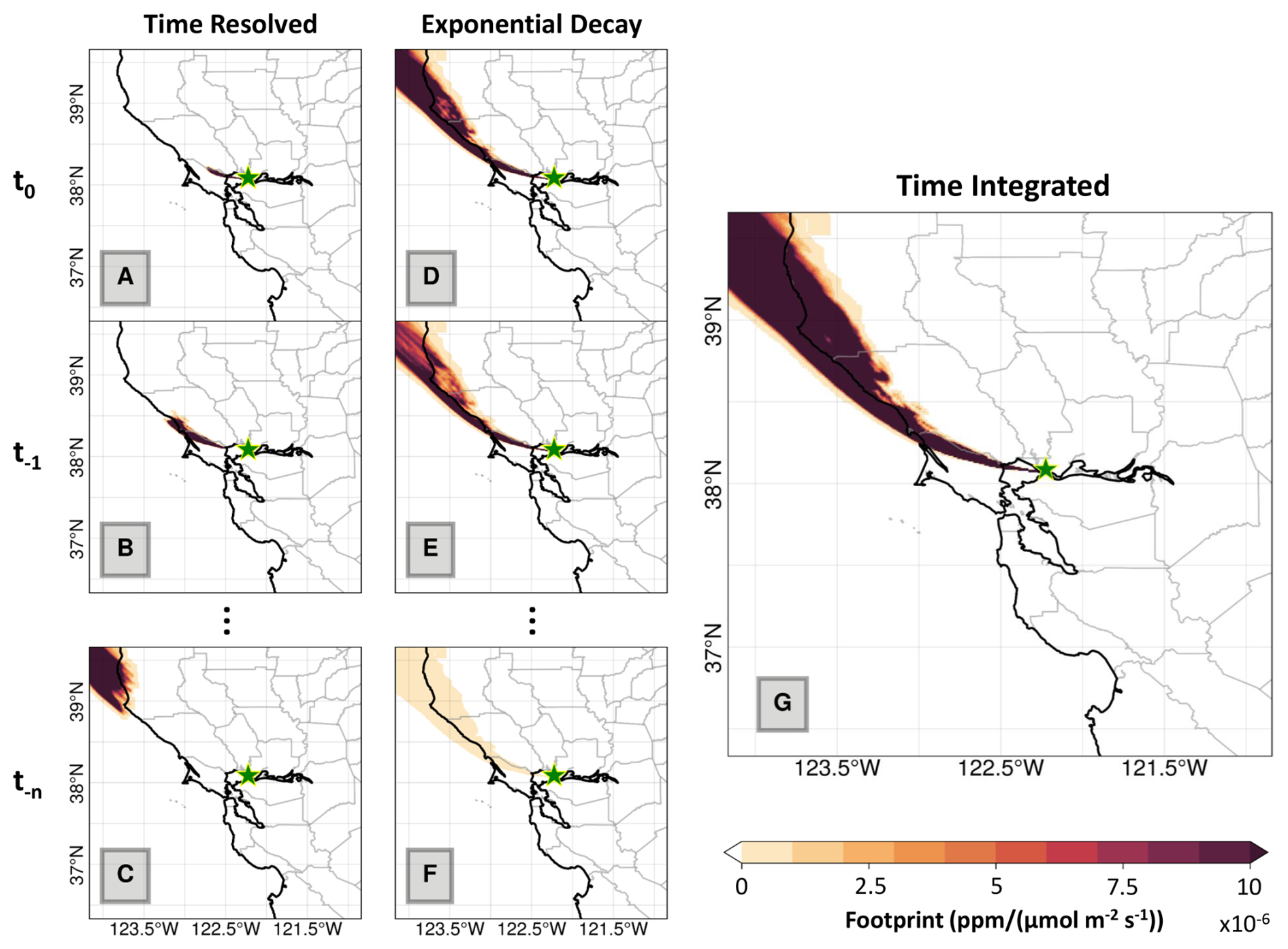
Figure 1 Two methods of representing temporal patterns in footprints for a single receptor. The green stars indicate the receptor location for the footprint. Panels (a) – (c) show the time-resolved footprints computed directly from STILT. Panels (d) – (f) show the time-integrated STILT footprints with the pattern allocated temporally using an exponential decay. Both representations have the same time-integrated spatial pattern (panel g).

Figure 1 shows the difference between hourly time-resolved footprints and the time-integrated footprints with exponentially decayed weights. The time-resolved footprints have a smaller sensitivity “blob” that moves as we go backward in time. This indicates that, for any given time step, only the emission sources in the small shaded region influence our observation. This highly time-resolved method assumes that the numerical schemes used for the transport and advection are highly accurate. In contrast, the time-integrated footprint with exponentially decayed weights assumes a time-invariant spatial structure with decreasing magnitude at previous time steps. This plume decays with time such that time steps close to the time of observation have higher weights as compared to the plume 72 h before the time of observation, which has negligible influence. This temporal allocation of the footprint will likely induce additional error.

We assess this error using a pair of flux inversions: (1) conduct a GHG flux inversion with time-resolved STILT footprints, and (2) conduct a second GHG flux inversion using STILT footprints where the footprints have been time-integrated and temporally allocated as described above. This pair of GHG flux inversions will isolate the impact of this temporal allocation. Please note that all other inversion parameters are the same between these tests.

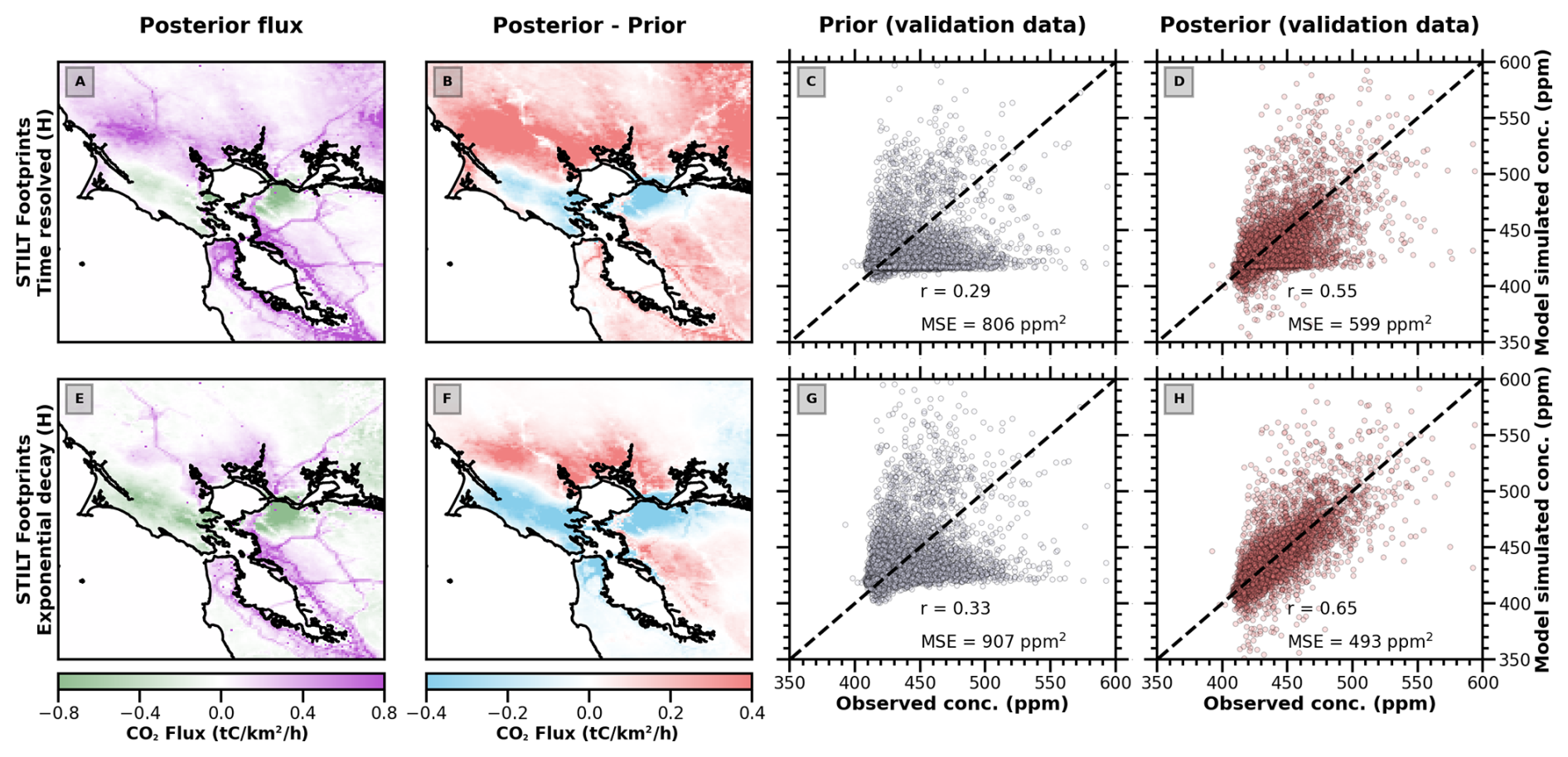
Figure 2 Comparison between CO₂ fluxes derived using time-resolved and time-integrated footprints with exponential decay for the STILT model. Panels (a)–(d) show flux inversion results using time-resolved footprints from STILT. Panels (e)–(h) show flux inversion results using time-integrated footprints with an exponential decay. Panels (a) and (e) show the posterior fluxes averaged over the study period from 2 February 2020 to 2 May 2020. Panels (b) and (f) show the difference between the posterior and prior fluxes. Panels (c) and (g) show a comparison of the model simulated concentrations using the prior fluxes against independent observations withheld from the flux inversion. Panels (d) and (h) show the same comparison as is panels (c) and (g), but using the posterior fluxes.

Figure 2 shows the results of these two GHG flux inversions in the Bay Area. It is important to emphasize that both of the inversions use the same set of footprints derived from the STILT model. The only difference is that one set of STILT footprints has been time-integrated and then reallocated temporally using exponential decay. The scatter plots compare observed CO₂ concentrations with the simulated CO₂ concentrations using prior and posterior fluxes on a validation dataset that was not used in the flux inversion. We use the same seed such that same validation concentrations are sampled in both cases. Overall, the posterior emission fluxes are in agreement. Interestingly, the second case, where the footprints have been temporally reallocated, does a better job at simulating independent observations with both the prior fluxes and the posterior fluxes. This can be seen in both the correlation and the mean squared error. Upon close examination of the scatter plots, it can be seen that the time-resolved scatter plots have a cluster of simulated concentrations around 410 ppm (approximately background signal), even though actual concentrations are higher than that. This pattern is visible in the CO₂ concentrations simulated using both prior and posterior fluxes. On the other hand, this pattern is not visible in the CO₂ concentrations simulated using the posterior fluxes of the exponential decay case.

The poor performance of the time-resolved footprints is likely driven by transport errors in the STILT simulations. The time-resolved footprints are a more realistic representation of the source–receptor relationship, but not necessarily more accurate. The simulated transport could have large biases that will propagate into time-resolved footprints. For example, errors in the wind speed could lead to parcels advecting too fast and attributing fluxes to the wrong spatial location. In these flux inversions, the ocean and the San Francisco Bay are assumed to be neither sources nor sinks. It seems that the sensitivity blobs in the time-resolved footprints are quickly advected over the ocean, and hence the simulated concentrations are closer to the background signal, even though the observed concentrations are higher. As such, the time-integrated footprints may be mitigating these transport errors and allowing GHG fluxes to be attributed correctly. Additionally, this pair of GHG flux inversions indicates that the exponential-decay-based temporal allocation of footprints should not induce significant errors in the GHG flux inversion. All of the GHG flux inversion experiments that follow (i.e., Sect. 5) will use FootNet footprints and this temporal allocation of the footprints.

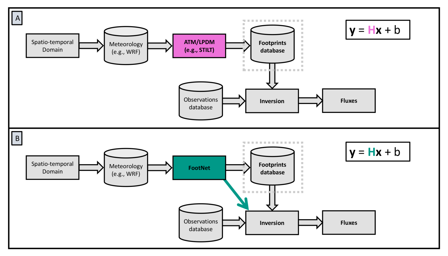
Figure 3 Conventional and FootNet-based GHG inversion frameworks. Panel (a) shows the conventional GHG flux inversion framework, which uses a full-physics LPDM simulation to compute footprints. Panel (b) shows the proposed GHG flux inversion framework using FootNet model to compute footprints. The arrow in panel (b) indicates how FootNet may be used to compute footprints on the fly as they are needed within the GHG flux inversion, bypassing the data storage step.

5 GHG flux inversions with a machine learning surrogate model

Using the temporal allocation strategy described above, we can now assess the performance of an ML-based surrogate transport model within a GHG flux inversion. Figure 3 shows conceptually how this ML model for atmospheric transport can be used within a GHG flux inversion. Figure 3a shows the conventional GHG inversion framework using an LPDM. This framework begins with obtaining meteorological data for the spatio-temporal region of interest. These meteorological data are used to drive the full-physics LPDM and, in turn, construct the footprints for all of the observations. Construction of these footprints is computationally expensive, and the footprints are typically archived prior to conducting the GHG flux inversion. Archiving these footprints can have large data storage requirements for dense observations at high spatio-temporal resolution. Following the construction and archival of the footprints, researchers can then estimate GHG fluxes via Bayesian inference, as described in Sect. 3.

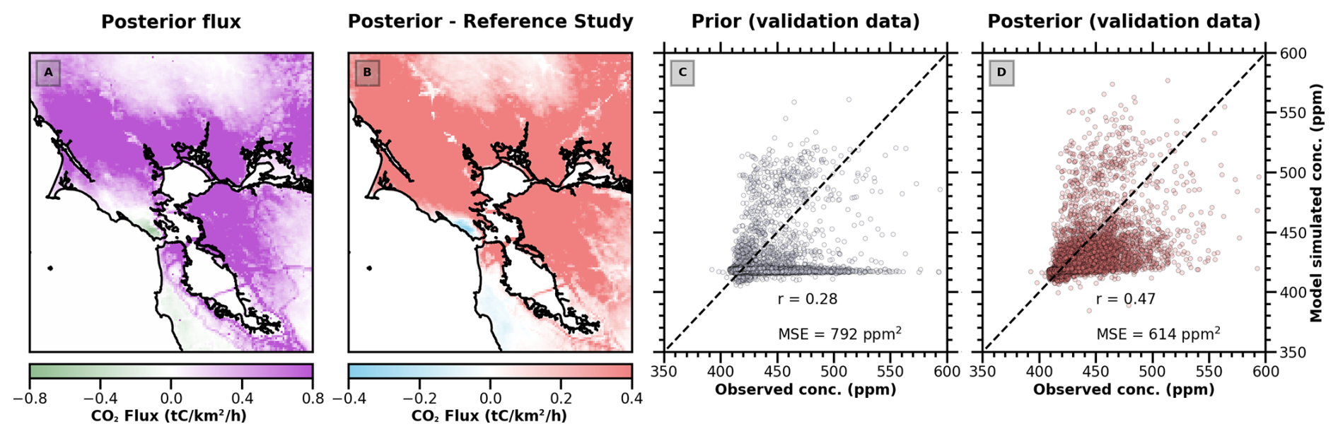
Figure 4 Urban CO₂ flux inversion results in the San Francisco Bay Area using FootNet v1 (He et al., 2025). Panel (a) shows the posterior CO₂ fluxes averaged over the study period. Panel (b) shows the difference between the posterior fluxes inferred with FootNet v1 and fluxes inferred with a full-physics model (STILT). Panel (c) shows a comparison of CO₂ concentrations simulated with FootNet v1 and the prior fluxes against independent observations. Panel (d) shows the same as in panel (c) but for posterior fluxes inferred from using FootNet v1. The reference study is Turner et al. (2020).

Figure 3b shows the process to estimate GHG fluxes using an ML model as a surrogate for the full-physics atmospheric transport model. The initial and final steps of the process are identical to the process described above. The difference is in the construction and archival of the footprints. We detail two approaches: (1) construct and archive the footprints, or (2) construct the footprints “on the fly” during the GHG flux inversion. The former approach is similar to the process using the full-physics model, but the construction of the footprints uses the ML-based surrogate model (e.g., FootNet). The latter approach of computing the footprints on the fly during the inversion is only feasible if the computation of the footprints can be done in near-real time; otherwise, additional computational expense would make the inversion prohibitively slow. The computation of a time-integrated footprint by the ML-based surrogate model described by He et al. (2025) takes less than a second and, as such, may be sufficiently fast to facilitate computation of footprints on the fly as they are needed in the GHG flux inversion. In the following sections, we evaluate the performance and the computational expense of GHG flux inversion frameworks using FootNet. These results will be compared to a GHG flux inversion using a full-physics atmospheric transport model (STILT).

5.1 GHG flux inversion with FootNet v1

Figure 4 shows the results of a flux inversion using FootNet v1, the model described in He et al. (2025), with the flux inversion setup from Turner et al. (2020), who evaluated the impact of COVID-19 regulations on urban CO₂ fluxes in the San Francisco Bay Area. Briefly, we conduct hourly flux inversions at 1 km spatial resolution for overlapping 96 h windows. Each 96 h window includes a 36 h buffer on the 24 h period of interest. The prior error covariance matrix is decomposed using a Kronecker product (e.g., Yadav and Michalak, 2013). Upwind concentrations are taken from NOAA observations in the Pacific and from AmeriFlux measurements in the Sacramento Delta.

From Fig. 4c and d, we observe that the posterior fluxes inferred using FootNet v1 perform substantially better than the prior fluxes when compared against independent validation data. Figure 4a shows changes in physically meaningful locations, such as freeways in the San Francisco Bay Area, as well as regions dominated by the biosphere. However, from Fig. 4b, we can see that these posterior fluxes do not appear to be in agreement with the fluxes inferred from Turner et al. (2020) using the full-physics model. FootNet v1 finds substantially higher fluxes throughout the domain than the inversion using the full-physics model. This suggests that FootNet v1 simulates realistic spatial patterns well but may be generating weaker footprints than STILT and may not be appropriately scaled. Additionally, the large differences in the far field seen in Fig. 4b indicate that there could be an imbalance between the near field and far field of the footprints from FootNet v1.

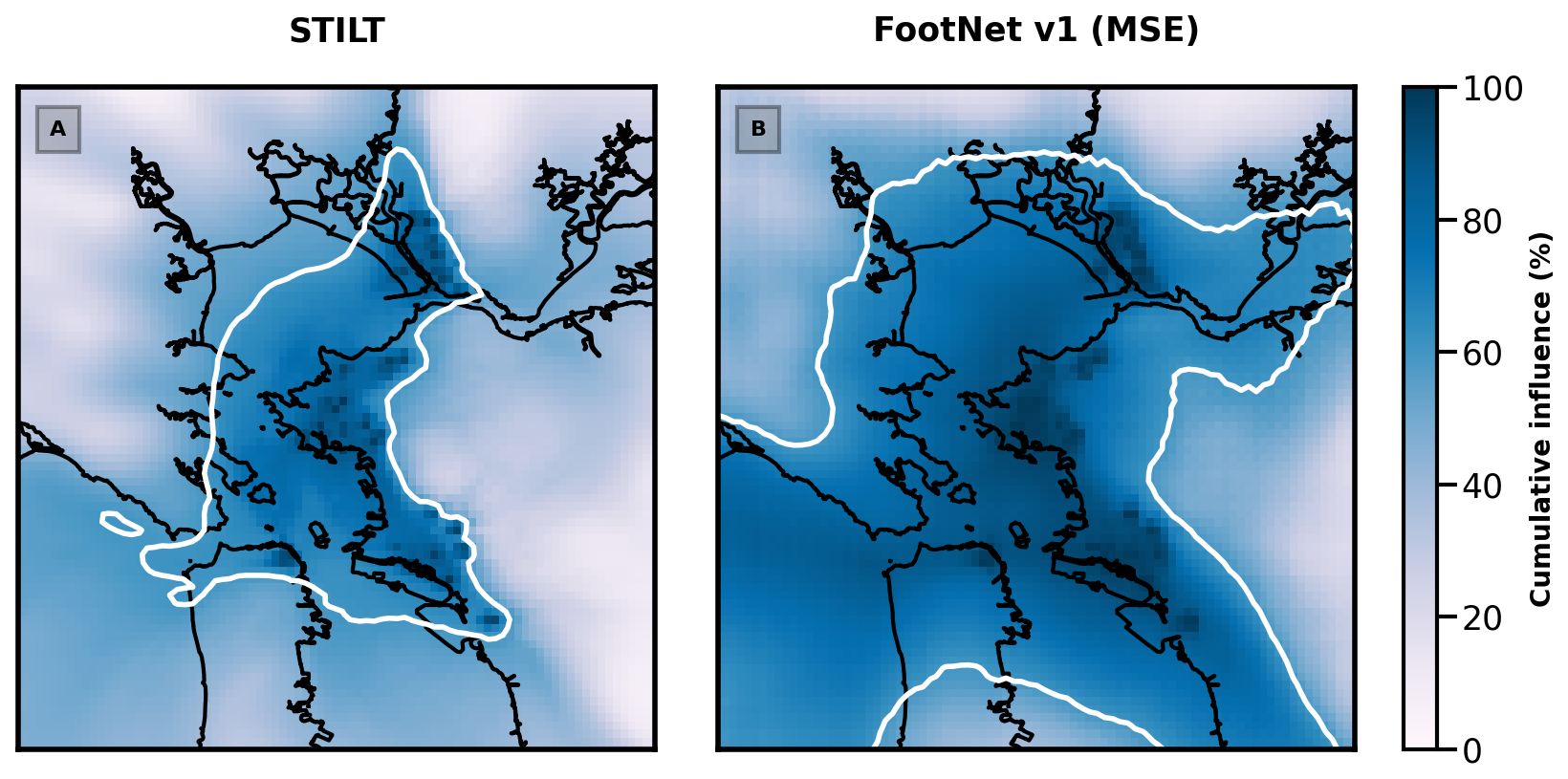
Figure 5 Cumulative region of influence for the BEACO₂N network in the San Francisco Bay Area. Panel (a) shows the cumulative influence computed using STILT, a full-physics model. Panel (b) shows the cumulative influence computed using FootNet v1 with an MSE cost function. The white contour represents the region encapsulating the top 40 % of the total influence on the BEACO₂N network (i.e., the region to which the observations are most sensitive).

Figure 5 shows the cumulative influence of footprints for the full-physics model (STILT) and FootNet v1. These cumulative influence plots give an idea of the spatial regions that the observations are sensitive to. As alluded to above, there are strong similarities in the spatial patterns, but FootNet v1 does indeed find a larger contribution from distant regions than STILT. This larger region of influence would result in FootNet allocating larger fluxes to distant regions than a flux inversion using STILT. This comparison of the regions of influence suggests that the FootNet model should be updated to improve the performance within a GHG flux inversion. We hypothesize two methods for improving the performance of FootNet: (1) changing parameters in the deep-learning architecture for FootNet and (2) adding input features to FootNet.

5.2 Updating the FootNet model to improve performance in flux inversions

As a first test, we train an additional variant of the FootNet model with an alternate formulation of the cost function (i.e., the cost function used to construct FootNet, not the cost function for a GHG flux inversion). This FootNet variant still relies on the underlying U-Net architecture. The FootNet v1 model used a mean-squared error (MSE; i.e., ℒ₂-norm) cost function in the gradient descent optimization. We hypothesize that an ℒ₁-norm cost function may improve the balance between the near field and the far field. This is because the MSE cost function is sensitive to outliers, in contrast to an ℒ₁-norm that is less sensitive to outliers (see Bishop, 2006).

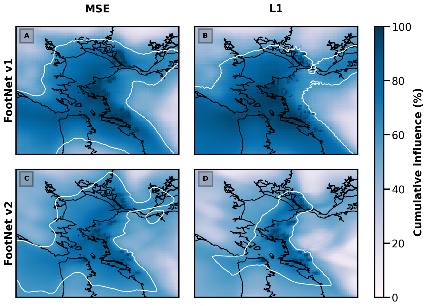
Figure 6 Same as Fig. 5 but for different variants of FootNet. Panels (a) and (b) show the cumulative influence for FootNet v1. Panels (c) and (d) show the cumulative influence for FootNet v2. Panels (a) and (c) use MSE cost functions. Panels (b) and (d) use ℒ₁-norm cost functions.

Figure 6a and b show the cumulative influence for FootNet v1 using both an MSE and ℒ₁ norm cost function. Both formulations of the cost function yield large spatial regions of influence. Based on this, we conclude that changing the cost function alone is insufficient to rectify the imbalance in the near-field and far-field footprints.

Two other FootNet model parameters we evaluate are the choice of activation function and the formulation of a log-transformation of the training data. The construction of FootNet v1 uses the rectified linear unit (ReLU) activation functions to introduce nonlinearity in the deep-learning model architecture (He et al., 2025). We assess the performance of parametric rectified linear unit (PReLU) activation functions. These PReLU activation functions have parameters that can be tuned during the training process, giving FootNet additional degrees of freedom. FootNet v1 also uses a logarithmic transformation of the training data to help identify large-scale spatial patterns. We modify the logarithmic transformation to add a small number and ensure positivity, as follows:

$$\begin{array}{}\text{(7)}& \mathrm{\Gamma }\left(x^{\ast }\right)=\log (x+\mathit{ϵ})-\log \left(\mathit{ϵ}\right),\end{array}$$

where x is a real number and ϵ is a small value ($\mathit{ϵ}={\mathrm{10}}^{-\mathrm{3}}$). Both of these updated parameter choices improved the performance of FootNet but did not fully rectify the near-field and far-field imbalance.

Table 1 Input features for FootNet.

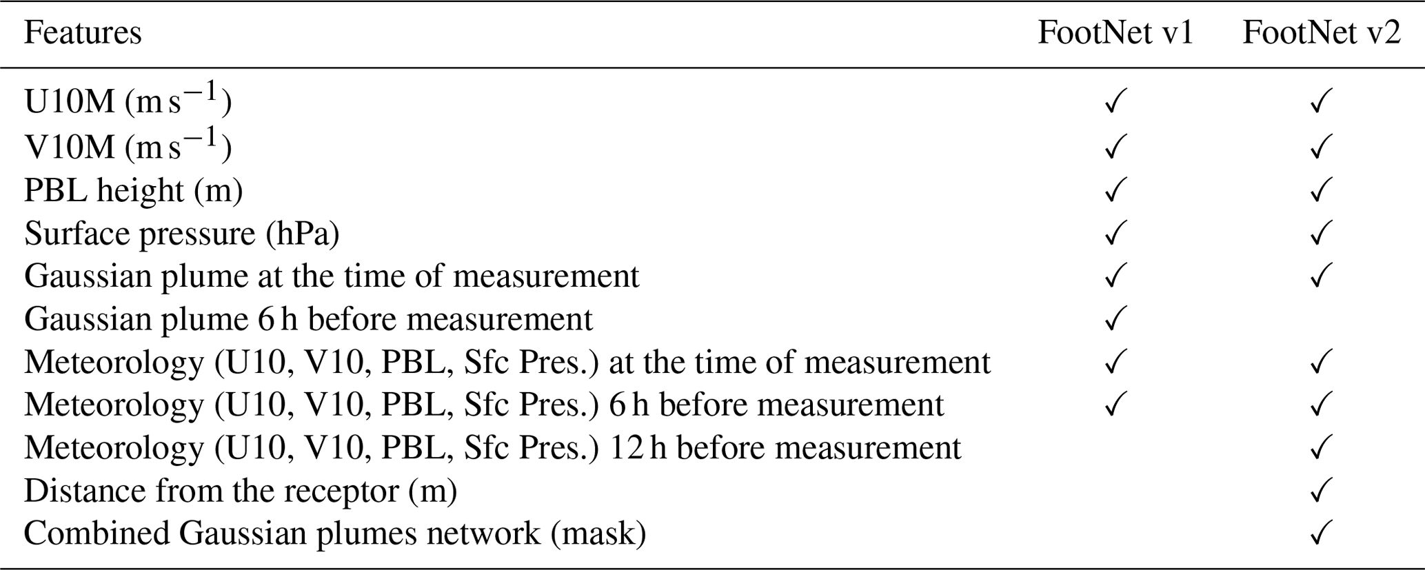
Finally, we trained two more FootNet models using additional input features shown in Table 1. We define these models with additional input features as “FootNet v2”. FootNet v1 only uses meteorological data at the time of measurement and 6 h prior. Here, we add meteorological data 12 h back in time. These meteorological data include 10 m zonal and meridional winds, surface pressure, and planetary boundary layer (PBL) height. Winds are important for the model to learn advection, and surface pressure also acts as a proxy for the region's topography. We also use PBL height, as it is an important input for computing footprints from the trajectories of the particles in a full-physics LPDM (e.g., STILT; Lin et al., 2003). The choice of 12 h is because many trajectories have not yet left the domain within 6 h, and, as such, meteorological information from 12 h before the observation time may be important in constructing the footprint and assessing fluxes. We also include distance from the receptor (both linear distance and an exponentially decaying distance). Distance from the receptor may help the model learn the optimal decay rate for the spatial pattern of the footprint (i.e., help the imbalance of the near field and far field). Finally, we include a spatial mask inferred from a network of Gaussian plumes. The spatial mask is based on winds at the time of measurement, 6, 12, 18, and 24 h back in time and may help identify the important regions influencing our measurement.

Figure 6 shows the cumulative influence plots for FootNet v2 using both MSE and ℒ₁-norm cost functions. The 60th percentile contours show a stronger resemblance to that of the full-physics STILT model (see Fig. 5a). The balance between the near field and far field is more in line with the cumulative influence inferred by the STILT model. As hypothesized, the model with the MSE cost function has a larger region of influence than the model using the ℒ₁-norm cost function. This allows the model to optimize the spatial decay structure of the footprints as it moves radially outward from the receptor location. Notably, the MSE-based cost function indicates a larger sensitivity over the ocean as compared to the STILT footprint and the ℒ₁-norm. This is likely due to FootNet simulating “smoother” footprints than STILT (STILT exhibits sharp gradients at the edge of the footprint). The FootNet v2 model using an ℒ₁-norm cost exhibits a smaller region of influence than the STILT model.

We can now assess the performance of the four models shown in Fig. 6 in the context of realistic GHG flux inversions. In all cases, the models will be compared against the results of GHG flux inversion using the full-physics STILT model (Turner et al., 2020), and they will be evaluated against validation data from CO₂ observations withheld from the flux inversion.

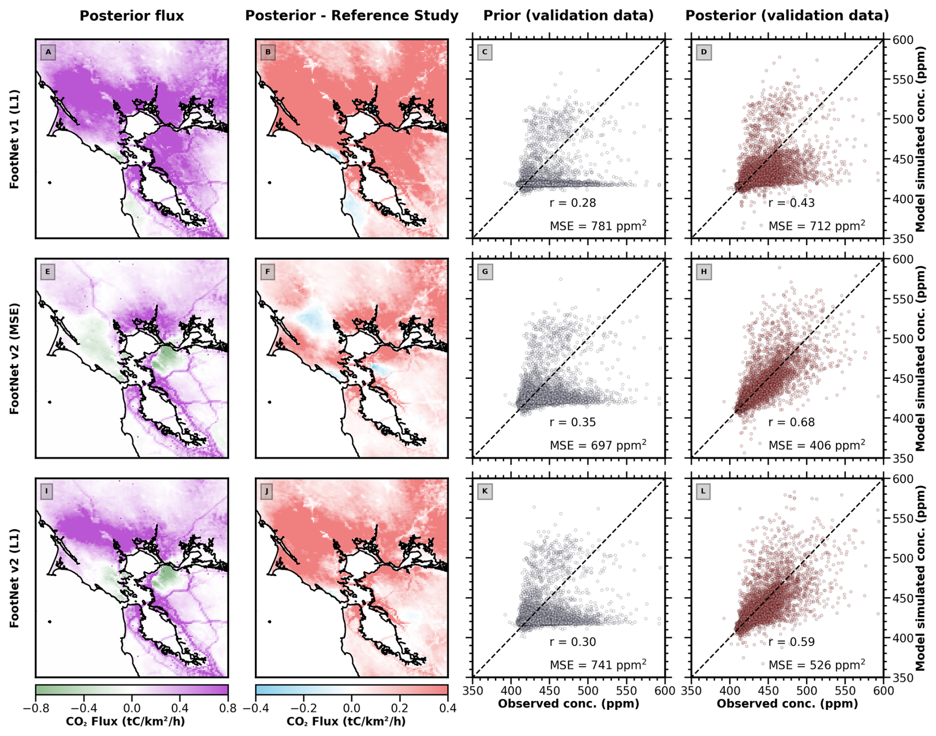
Figure 7 Same as Fig. 5 but for three other variants of FootNet: FootNet v1 trained with an ℒ₁-norm cost function (a–d), FootNet v2 trained with an MSE cost function (e–h), and FootNet v2 trained with an ℒ₁-norm cost function (i–l). The reference study is Turner et al. (2020).

Figure 7 shows the comparison of these models against Turner et al. (2020) and the validation data (note, one of the cases is shown above in Fig. 4). As shown in Fig. 6, the near-field and far-field imbalance persists in FootNet v1 using an ℒ₁-norm cost function. Both variants of FootNet v2 show marked improvement in the near-field and far-field balance. Additionally, both variants of FootNet v2 perform substantially better against independent validation data (see right column). Between the two variants of FootNet v2, we find that the mean squared error (MSE)-based cost function performs best. This conclusion is based on the performance against independent validation data and comparison to the posterior fluxes from Turner et al. (2020). The comparison against independent validation shows a strong correlation (r=0.68) and no systematic biases in the residuals. The mean squared error against independent validation data is the lowest of the FootNet models tested (MSE = 405 ppm²). FootNet v2 with an MSE cost function also shows the smallest deviations from the posterior fluxes inferred from Turner et al. (2020), who used a computationally expensive full-physics model to relate the fluxes to observations. As such, we select FootNet v2 with an MSE cost function as the final model.

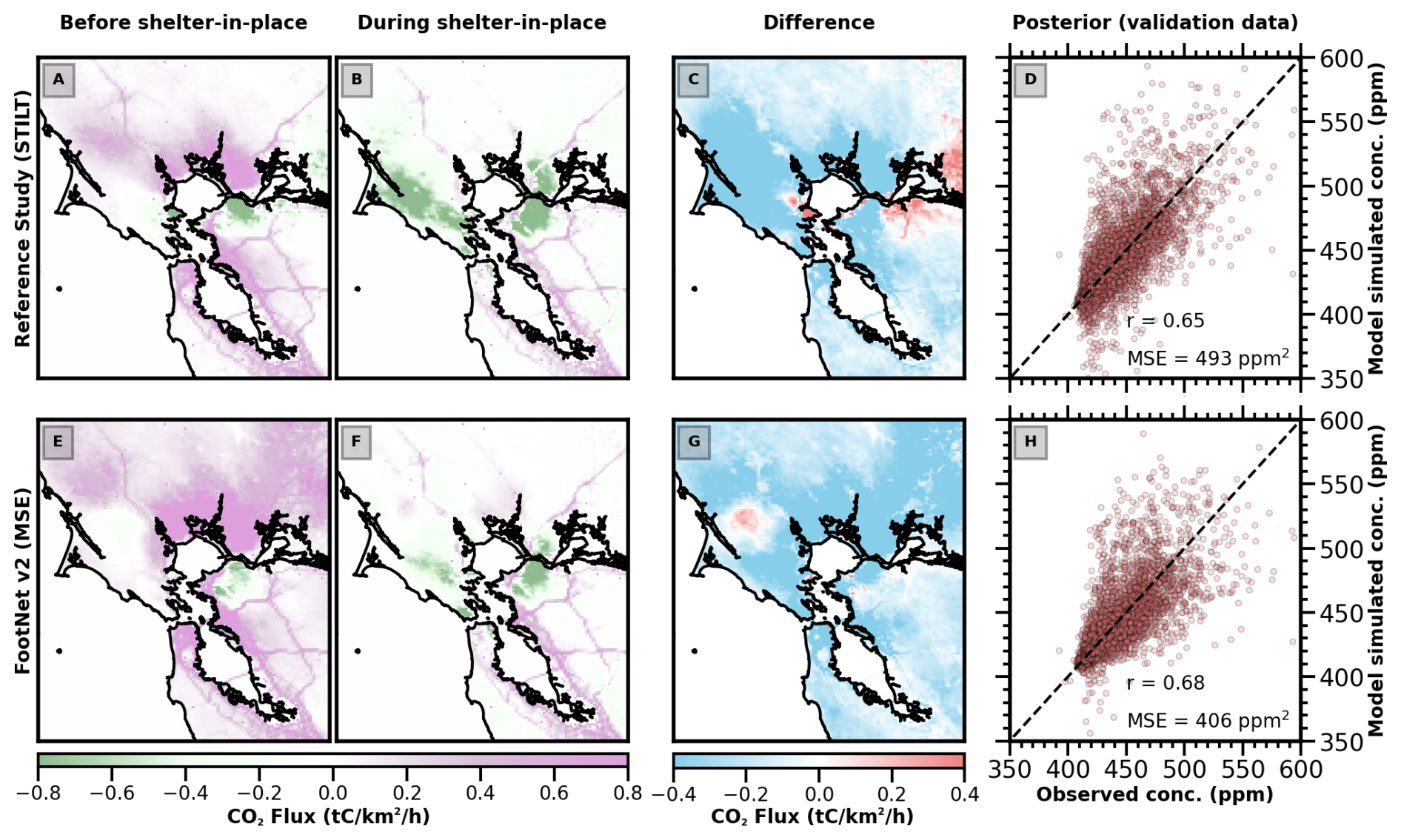
Figure 8 Urban CO₂ fluxes in the San Francisco Bay area inferred using atmospheric observations. Panels (a)–(d) show the posterior CO₂ fluxes inferred using footprints from STILT, a full-physics transport model. Panels (e)–(h) show the posterior CO₂ fluxes inferred using FootNet v2 with an MSE cost function. Panels (a) and (e) show the CO₂ fluxes averaged over 6 weeks before the COVID-19 shelter-in-place orders. Panels (b) and (f) show the CO₂ fluxes averaged over 6 weeks during the COVID-19 shelter-in-place order. Panels (c) and (g) show the difference between these time periods. Panels (d) and (h) compare predicted CO₂ concentrations using the posterior fluxes with independent CO₂ observations withheld from the flux inversion. Note that both inversions use time-integrated footprints that have been temporally allocated based on an exponentially decaying weight.

Figure 8 shows a direct comparison of FootNet v2 using an MSE cost function against the posterior fluxes inferred from Turner et al. (2020) using a full-physics model (STILT). The comparison shows the average fluxes for 6 weeks before COVID-19 shelter-in-place orders, 6 weeks during shelter-in-place orders, the difference, and a comparison against independent validation data. Figure 8a and e show a strong similarity in their CO₂ fluxes before the COVID-19 shelters were in place. We note some disagreements in the far field, such as the northern and eastern parts of the domain. Figure 8b and f correspond to the period during the shelter-in-place measures that decreased anthropogenic emissions. Both sets of posterior fluxes are in agreement during this period, with clearly visible reductions in emissions from freeways and anthropogenic sources. The only notable difference is near Tomales Bay and Point Reyes, in the western portion of the domain. Figure 8c and g show the difference in the CO₂ fluxes between these two periods. Both inversions largely agree in the Bay Area, where the observations have the largest influence. Some disagreements can be seen to the east of Tomales Bay and in the Sacramento Delta. Finally, the right column of Fig. 8 shows the comparison against independent validation data for both flux inversions. Interestingly, we observe the FootNet v2 posterior fluxes to perform better than the posterior fluxes inferred using STILT. This is seen in both the correlation coefficient (r=0.68 for FootNet and r=0.65 for STILT) and mean squared error (MSE = 405 ppm² for FootNet and MSE = 493 ppm² for STILT). This begs the question: “why would a machine learning surrogate model perform better than the full-physics model in a GHG flux inversion?”

FootNet was designed to emulate the STILT model (a full-physics atmospheric transport model); as such, it is surprising to see the ML-based surrogate model outperform the full-physics model it was trained on when used in a GHG flux inversion. The explanation for this paradox is that, while STILT is a more realistic representation of the transport it is not necessarily more accurate. ML models often give predictions that tend toward the mean. In the context of atmospheric transport and footprints, this results in a FootNet simulating a smoother and more diffuse spatial pattern than STILT (He et al., 2025). When used in a GHG flux inversion, the sharp gradients simulated with STILT mean that small errors in wind speed or direction could lead to fluxes being allocated to the incorrect spatial location. In the context of the GHG flux inversion, this diffuse spatial pattern simulated by FootNet can potentially mitigate transport errors in the flux inversion. An important takeaway from this work is that using an ML-based surrogate model in a flux inversion can potentially outperform the computationally expensive full-physics model. However, this result is unlikely to be universally true, as there will be cases where smoother spatial patterns induce errors in the flux inversion (e.g., when the true trajectories are localized). The performance of the ML-based surrogate model will almost certainly vary on a region-by-region basis, and additional tests are needed to assess the extent of this finding.

Table 2 Construction and storage cost to compute footprints with STILT and FootNet^a.

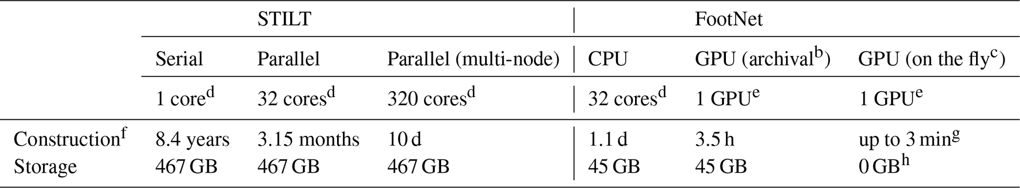
^a Computation times may change slightly based on factors such as hardware usage and resource availability. ^b Flux inversion using archived footprints. ^c Footprints computed as they are needed during the flux inversion. ^d Intel^® Xeon^® Gold 6226R CPU @ 2.90 GHz. ^e NVIDIA A2 GPU, 16 GB GDDR6. ^f Constructing 73 703 footprints. ^g ∼ 800 observations for a 1-day inversion with a 96 h window. ^h No archival of footprints in the on-the-fly framework.

6 Computational cost of the GHG flux inversions

Table 2 shows the computational and storage cost analysis for both STILT and FootNet v2 for the 3-month study period. The construction of footprints for all of the measurements using the full-physics-based STILT model is computationally expensive. It takes roughly an hour (upper bound) to construct a single footprint using STILT. As such, it can take more than 8 years to construct all the footprints required for this study if one were to construct them sequentially. Parallel computation of the footprints on a 32-core machine can reduce the time to 3 months. Using multiple nodes can further reduce the time to a few days. However, this reduction in time comes with an infrastructure cost. Given the computational expense in generating these footprints, researchers typically store these time-resolved footprints, which can take approximately 470 GB of space for this study period.

The computation of footprints using FootNet v2 is fast. It takes 3.5 h to compute the same footprints using a single NVIDIA A2 GPU card on 1 core and 24 h using a 32-core machine; this is a 650 × and 85 × speedup on similar hardware, respectively. This time includes reading input data, constructing footprints, and writing to disk. He et al. (2025) mention that it takes 0.08 s to compute a single footprint after loading input data. This speedy computation from FootNet allows for near-real-time construction of footprints within the GHG flux inversion. In other words, one can compute footprints on the fly as they are needed, rather than storing the footprints on the disk. Additionally, it may allow researchers to conduct sensitivity runs on meteorological parameters (e.g., the PBL height) during the flux inversion by including meteorological parameters as a hyperparameter in the inversion. We note that the storage cost is lower for FootNet because STILT is saving time-resolved footprints.

The serial computation of the HB matrix, based on the computationally efficient algorithm proposed by Yadav and Michalak (2013), can also become computationally expensive. In this study, we implemented a parallel computation of HB matrix based on the algorithm detailed in Yadav and Michalak (2013). This parallel implementation is approximately 27 times faster than the serial implementation. Appendix A discusses the parallel implementation of HB matrix computation.

7 Conclusions

Near-real-time quantification of greenhouse gas (GHG) fluxes is important for monitoring, reporting, and verification of GHG fluxes to ensure climate goals are met. Here we demonstrate how machine learning (ML) models can be used as a surrogate for the full-physics atmospheric transport models in a GHG flux inversion, alleviating a computational bottleneck. This work updates the deep-learning architecture of FootNet v1 (He et al., 2025) to improve the performance in a GHG flux inversion. This updated deep-learning model for atmospheric transport (FootNet v2) outperforms the full-physics model in an inversion estimating urban CO₂ fluxes at high spatio-temporal resolution in the San Francisco Bay Area. Further tests are required to investigate the generalizability of this finding.

A potential barrier to using FootNet within a GHG flux inversion is that FootNet computes a 2-D spatial pattern of time-integrated footprints, whereas the full-physics model (STILT) generates time-resolved footprints. To overcome this, we temporally allocate the footprints using an exponentially decaying weight such that there is a time-invariant spatial structure with decreasing magnitude at previous time steps. Further, we compare predicted concentrations after conducting flux inversion using both the time-resolved and time-integrated footprints with temporal allocation. We observe that time-integrated footprints perform better, as they can mitigate transport errors in the time-resolved representation. The time-resolved footprints are a more realistic representation of the source–receptor relationship, but not necessarily more accurate. Additional tests are needed to understand the transport errors in the time-resolved footprint and the broader applicability of the exponential-decay footprints. This overcomes a potential barrier to using the ML-based surrogate model in a flux inversion.

A preliminary flux inversion using FootNet v1 suggested there was a bias in the balance between the near-field and far-field footprints. We constructed additional variants of the FootNet model and evaluated them in an urban CO₂ flux inversion. Performance was evaluated against independent observations that were withheld from the flux inversion. Ultimately, we developed a new model (FootNet v2) that includes additional input features. We find that FootNet v2 outperforms the full-physics model in the flux inversion in this particular study. This is likely because the FootNet v2 footprints have a smoother spatial structure than the full-physics model. This smoother spatial structure can help mitigate transport errors. Additionally, this machine learning surrogate model allows for a 650× speedup in the construction of the footprints as compared to the full-physics model. This speedup allows for on-the-fly computation of footprints during the inversion, as opposed to archiving footprints prior to the GHG flux inversion.

Previous work has shown that the distribution of GHG sources may be skewed, with a “heavy tail” of super emitters. This suggests that the assumption of a Gaussian distribution for the prior PDFs may not be accurate. Stochastic methods such as Markov chain Monte Carlo can allow one to specify non-Gaussian prior PDFs, as well as jointly solve for meteorology (e.g., uncertainties in PBL height). However, it is currently infeasible to implement with traditional models, as it requires evaluation of the forward model many times, which is computationally intractable. FootNet can compute the footprints in near real time, making it feasible to use these methods to estimate posterior emissions. This can be one potential application of machine learning surrogates of atmospheric transport in improving the flux estimates.

Overall, FootNet alleviates a computational bottleneck when working with dense GHG observing systems, such as those from urban monitoring networks and next-generation satellite measurements (e.g, MethaneSat and Carbon-I). The computational efficiency of FootNet allows for near-real-time emission monitoring of GHGs, along with other nonreactive trace gases. This work demonstrated the utility of FootNet in quantifying urban CO₂ fluxes in a case study, and future work is needed to extend this framework to a larger region, such as the contiguous US, or total column measurements. Nevertheless, ML-based surrogate models such as FootNet represent a promising direction for efficiently interpreting the growing volume of observational data from next-generation observing systems.

Appendix A: Parallel implementation of HB matrix multiplication

Here, we use a shared-memory parallelization technique to compute HB from H_n×pr, the temporal prior error covariance matrix (D_p×q), and the spatial prior error covariance matrix (E_r×t). This method is similar to the algorithm described in Yadav and Michalak (2013). The primary difference from Yadav and Michalak (2013) is that we form HB in shared memory and use a multi-threading approach to iterate over the q columns of D simultaneously, such that a thread performs the following operation on the kth column of D:

1. Multiply each (n×r) block of H by the elements of the kth column of D and add these blocks.

2. Multiply the resulting n×r matrix by E_r×t to obtain the kth n×t column block of HB matrix.

3. Update the kth n×t column block of HB matrix.

4. End the thread operation.

This method is limited by the number of threads and the memory available for the matrix multiplication. The larger the number of threads, the faster the multiplication can be, provided that there is enough memory available for each thread.