Surface ozone trend variability across the United States and the impact of heat waves (1990–2023)

This paper outlines a comprehensive trend assessment of surface ozone observations across the conterminous USA over 1990–2023. A change point detection algorithm is applied to evaluate seasonal trends at various percentiles. We found that highly consistent and robust negative trends in extreme values have occurred in spring, summer, and fall since the 2000s across the eastern USA. A less strong but similar picture is found in the western USA, while increasing winter trends are commonly observed in the Southwestern and Midwestern regions of the country. The impact of a potential climate penalty that might offset some of the improvement in the ozone extremes is also investigated based on various heat wave metrics. By comparing ozone threshold exceedances, we found that the exceedance probabilities during heat waves are higher than those under normal conditions; moreover, the differences have decreased over time, as the effectiveness of emission controls has led to a great reduction in ozone extremes under both heat wave and normal conditions. When the increasing heat wave trends are accounted for, we find evidence that decreases in exceedances during heat waves have likely halted at 20 %–40 % of sites, depending on heat wave definitions. By identifying monitoring sites with (1) reliably decreasing ozone exceedances and (2) reliably increasing co-occurrences of ozone exceedances and heat wave events, we can show that several sites in California have been impacted by the ozone climate penalty (1995–2022). These findings are limited by the availability of long-term continuous ozone records, which are sparsely distributed across the USA and typically less than 30 years in length.

1 Introduction

Surface ozone is an air pollutant that is detrimental to human health (Fleming et al., 2018) and crop production (Mills et al., 2018); it is also an important greenhouse gas (Gaudel et al., 2018). The United States (US) Clean Air Act of 1970 requires the US Environmental Protection Agency (EPA) to set National Ambient Air Quality Standards (NAAQS) for ozone. The standards have been reviewed and updated regularly to protect the public health and welfare. The current primary standard established in 2015 and reviewed in 2020 is 70 ppbv for the fourth-highest daily maximum 8 h ozone average (MDA8) value, averaged over 3 consecutive years (US EPA, 2020b).

The EPA Air Quality System (AQS) monitoring network provides extensive long-term surface observations of air pollutants and meteorology (US EPA, 2024a). These data have been constantly studied to quantify the impacts of air pollution on air quality metrics, human health, and vegetation, and the data are also relevant to climate assessments (Cooper et al., 2014; Simon et al., 2015; Fleming et al., 2018; Jaffe et al., 2018; US EPA, 2020a; Wells et al., 2021). This dataset is also an important source for evaluating chemistry–climate models and satellites (Rasmussen et al., 2012; Fiore et al., 2014; Zoogman et al., 2014). Several studies have reported a reduction in surface ozone across much of the USA since the early 2000s in response to ozone precursor emission controls (Cooper et al., 2012; Simon et al., 2015; Strode et al., 2015; Seltzer et al., 2020), in which the decreases in the eastern USA are often clearly demonstrated (Chang et al., 2017; Lin et al., 2017). Ozone across the western USA is more challenging to quantify on a regional scale due to the complex terrain, relatively sparse monitors, and impacts from wildfires and oil and gas emissions (Edwards et al., 2014; Lu et al., 2016; McDuffie et al., 2016; Parks and Abatzoglou, 2020; Francoeur et al., 2021; Buchholz et al., 2022; Langford et al., 2023; Peischl et al., 2023; Putero et al., 2023; Byrne et al., 2024; Marsavin et al., 2024; Sorooshian et al., 2024), but overall decreasing trends can be detected across the Southwestern USA (Chang et al., 2021) and at high-elevation rural sites (Chang et al., 2023a).

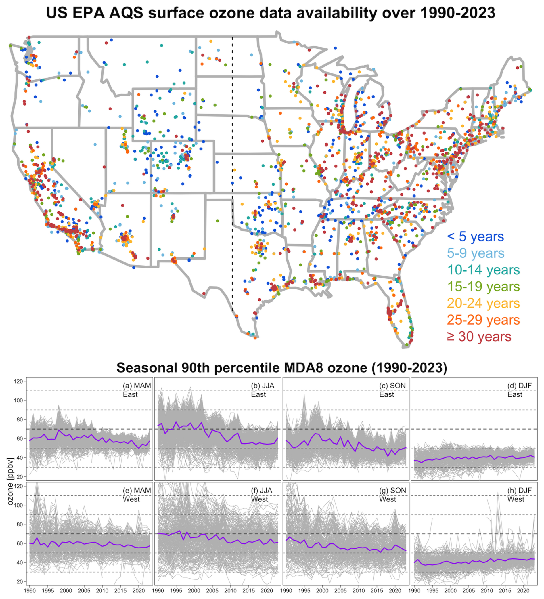
Figure 1 The upper panel shows the data availability of the EPA AQS surface ozone observations over 1990–2023; a total of 2540 sites are shown. The lower panel shows MDA8 time series at the seasonal 90th percentile: observations from individual stations are shown in gray; simple averages are shown in purple.

In terms of statistical modeling, tropospheric ozone variability is inherently heterogeneous in space and time. Regional trend detection of surface ozone is also complicated by the irregular distribution of monitoring sites, different lengths of site records, and varying spatial coverage over time (see Fig. 1 for surface ozone data availability). In the first phase of the Tropospheric Ozone Assessment Report (TOAR), a regional trend assessment for the eastern USA was conducted within the framework of the generalized additive mixed models (GAMMs) and focused on the summertime period (April–September) over the span from 2000 to 2014 (Chang et al., 2017). In this study, we present an extensive long-term seasonal trend assessment of surface ozone observations over the period from 1990 to 2023 and aim to tackle additional challenges, including (1) greater attention to the trends in ozone extremes, such as the extreme percentiles and threshold exceedances, and (2) evaluation of potential change points in long-term trends. Both challenges are addressed at local (individual sites) and regional scales.

While anthropogenic emission controls lead to decreasing average and extreme ozone levels, outstanding concerns remain, such as the contributions of heat waves and wildfires to ozone production (Jing et al., 2017; Lin et al., 2017; Langford et al., 2023; WMO, 2023; Cooper et al., 2024). The Intergovernmental Panel on Climate Change (IPCC) Sixth Assessment Report concluded that it is virtually certain that the frequency and intensity of hot extremes and the intensity and duration of heat waves have increased since 1950 and will continue to increase as the planet warms (Arias et al., 2021). Heat waves provide ideal conditions for the photochemical production of ozone due to sunny skies, low wind speeds, and a capped boundary layer height. Although the co-occurrence of heat waves and ozone extremes has been identified previously (Schnell and Prather, 2017), its co-variability is difficult to explicitly quantify, particularly when coupled with rapid emission reductions. The deterioration of ozone air quality due to increasing temperatures caused by climate change is known as the “climate penalty” (Wu et al., 2008; Zanis et al., 2022). Projections of climate change over the 21st century suggest that a clear ozone climate penalty (annual average ozone increases of 1–3 ppbv) could emerge in high-emission regions, such as northern India and eastern China, in association with large temperature increases (3 °C above 1850–1900 temperatures) and on timescales of more than 40 years (Zanis et al., 2022; WMO, 2022). A final objective of our analysis is to determine if any long-term ozone monitoring sites in the USA show evidence of a climate penalty over the relatively short timescale of 1995–2022. Recognizing that detection of a climate penalty could require relatively large temperature increases, we focus on heat wave conditions during the warmest months of the year (May–September). We aim to quantify the heat wave impact on ozone variability by comparing ozone exceedance trends between heat wave and normal conditions, using rigorous and widely adopted heat wave metrics (Perkins et al., 2012; Perkins and Alexander, 2013).

The trend detection framework of seasonal ozone percentiles and exceedances is described in Sect. 2. We quantify surface ozone trends at individual stations and the overall regional trends across the western and eastern USA over the period from 1990 to 2023 in Sect. 3. After the current status of ozone trends and variability are better understood, we further discuss the potential climate penalty for ozone extreme events in Sect. 4, i.e., the heat wave impact on short-term ozone variability and long-term exceedance trends. Conclusions are presented in Sect. 5.

2 Data and methods

Because of differences in the sensitivity of ozone to precursor emissions, different monitoring sites might respond dissimilarly, in terms of the latency and magnitude of trend changes at different percentiles and seasons (Box and Tiao, 1975). As the presence of a trend change is suspected but its juncture is unknown, additional care needs to be taken. In this section, we introduce the metrics for studying extreme ozone events, discuss the rationale for change point detection, describe the statistical methods for detecting trends at individual sites, and provide further considerations for deriving representative regional trends.

2.1 Ozone and heat wave metrics

Two types of extreme data are typically present in statistics: block maxima and threshold exceedances. The block maxima approach, which is not based on a particular standard, originally focuses on the maximum value at each time interval (a block indicates a selected time unit, e.g., a time series of seasonal ozone maximum values; Smith, 1989). As the concept of extreme percentiles (e.g., 90th) is closely related to the block maxima, to avoid confusion and to represent a wider range of extreme events, we use the term block extremes hereafter. Threshold exceedances, also known as the “peak over threshold”, make a binary classification of data into relevant (events occur) and irrelevant (events do not occur) categories.

In this study, all of the ozone analyses are based on daily maximum 8 h average (MDA8) values available from the US EPA AQS network (US EPA, 2024a). It should be noted that TOAR uses the mole fraction of ozone in air (nmol mol⁻¹) to describe the mixing ratio of an ozone observation. In contrast, in order to maintain consistency with the human health research community, the units of parts per billion by volume (ppbv) are used to report MDA8, as recommended by the TOAR guidelines. The particular ozone metrics for block extremes are the 10th and 90th percentiles of MDA8 in each season (in addition to the seasonal medians); for threshold exceedances, the ozone metrics are the number of days per summertime period in which the MDA8 value exceeds various thresholds, mainly limited to the period between May and September (as we aim to compare the ozone exceedances between heat wave and normal conditions). In addition to a threshold of 70 ppbv for the US EPA NAAQS, we also report the threshold exceedances based on 60 and 50 ppbv (commonly used to represent non-attainment occurrences for some air quality standards adopted globally; WHO, 2006; European Commission, 2015; US Federal Register, 2015) and on 35 ppbv (recommended by the World Health Organization to assess ozone health impacts; WHO, 2013). Note that the statistical characteristics are different for percentile data (continuous variable) and exceedance days (count variable), so different statistical methods are required (see Sect. 2.3).

To present the actual extreme ozone variability, the lower panel of Fig. 1 shows the seasonal 90th percentile time series from individual stations in the western and eastern USA (based on the 100° W boundary). While ozone has generally decreased over the period from 1990 to 2023 in MAM (March–April–May), JJA (June–July–August), and SON (September–October–November), we can see tumultuous variability within regions and differences between regions. For example, reductions in ozone extremes are obvious in the eastern USA, where exceedances of 70 ppbv were commonly observed before the early 2000s but became infrequent after 2013. In contrast, in the western USA, strong ozone extremes have been common in recent years, and ozone exceedances can also be observed in DJF (December–January–February), mainly in the snow-covered oil and gas basin of northeastern Utah (Fig. S1 in the Supplement) (Edwards et al., 2014). These features are expected to be the key factors to determine the resulting trends and uncertainty. Nevertheless, this is merely one aspect of the complexity, and full demonstrations of heterogeneous ozone variability for other percentiles (10th and 50th) are provided in Figs. A1 and  A2. These demonstrations clearly indicate that summarizing multiple aspects of ozone variability is essential for delivering a comprehensive trend assessment.

The NOAA Physical Sciences Laboratory (PSL) and Climate Prediction Center's global unified temperature dataset (NOAA PSL, 2024) provides gridded daily temperatures at a 0.5° × 0.5° resolution. These gridded temperatures are interpolated to all the ozone monitor locations (interpolation details are provided in Sect. 2.4) and are used to determine heat wave events at each location. The heat wave metrics used in this study are adopted from well-established heat wave research literature (Perkins and Alexander, 2013; Mazdiyasni and AghaKouchak, 2015; Domeisen et al., 2023). Firstly, given daily maximum (T_max) and minimum (T_min) temperatures, the following temperature thresholds are considered:

1. TX90pct. This threshold is the 90th percentile of a 15 d moving window of T_max (centered at each calendar day); each calendar day has a different percentile value (analogous to the seasonal climatology). This is the constant temperature baseline at each grid cell or monitoring location, against which heat wave events (i.e., temperature exceedances) are defined.

2. TX95pct. TX95pct is the same as TX90pct but based on the 95th percentile.

3. TX35deg. This is a fixed threshold at 35 °C for T_max.

4. TN90pct. TN90pct is the same as TX90pct but based on T_min.

5. TN95pct. TN90pct is the same as TN90pct but based on the 95th percentile.

6. TN20deg. This is a fixed threshold at 20 °C for T_min.

For each temperature threshold described above, a heat wave event is detected if at least 3 consecutive days of corresponding exceedances are found. Thus, a total of six heat wave metrics are considered based on long-term temperature data. A longer period of gridded temperature data (1990–2022) is used to better determine the temperature percentiles. While both T_max and T_min are important indicators to identify potential heat waves (Perkins and Alexander, 2013), there is a lack of previous studies addressing the sensitivity of MDA8 exceedance trends based on different heat wave definitions. Although we would expect that a higher T_max is typically better correlated with ozone extremes (Porter et al., 2015; Wells et al., 2021), a high temperature threshold might prevent us from having sufficient sample sizes for valid statistical analysis. Therefore, (i) TX35deg represents a fixed threshold, but this threshold is considerably too high for middle- and high-latitude sites; (ii) TX95pct and TX90pct enable sufficient observations for studying heat waves, as these thresholds are site-specific; and (iii) TX95pct provides a warmer condition than TX90pct for ozone production and can be considered to be a trade-off between TX35deg and TX90pct. In summary, albeit with a much smaller number of sites that can quantify the TX35deg condition, our results show a general similarity between different metrics (see Sect. 4 for more in-depth discussions).

In order to investigate the heat wave impact on instantaneous ozone variability, two (short-term) statistics during heat waves are considered for each site: (1) ozone enhancement (in units of parts per billion by volume, ppbv), which is a simple MDA8 mean difference between heat wave and normal conditions, based on deseasonalized anomalies; and (2) ozone accumulation rate (in units of parts per billion by volume per day, ppbv d⁻¹), which is designed to quantify the daily rate of ozone change (if any) throughout the durations of the heat wave. The accumulation rate is our quantity of interest, because it indicates if a longer heat wave produces higher ozone concentrations. It should be noted that the initial ozone conditions are different for each heat wave event, so it is necessary to adjust the ozone initial level between different events. This approach is also known as the random intercept model (i.e., intercepts vary for each heat wave event, but the slope or accumulation rate is invariant). Statistically, let m_ij be the MDA8 value and h_ij be the corresponding temporal index at the ith day from the jth heat wave event at a given site; the model can then be expressed as follows: $m_{ij}=(a+u_j)+b{h}_{ij}+\text{residuals}$, where a is the overall intercept, u_j is the adjustment of the initial condition for the jth heat wave event, and b is the daily accumulation rate during the heat wave. This model is similar to trend analysis but aligned to heat wave periods over several days (invariant to different time periods).

2.2 Change point detection applied to a large database of ozone time series: practical considerations

Many change point detection methods have been developed to evaluate optimized change point(s) and to model the nonlinear trends parametrically (see reviews by Reeves et al., 2007, and Lund et al., 2023, and comparisons by Chen et al., 2011, and Shi et al., 2022). While those methods are practical, a visual diagnosis of the time series plot is often required to validate the reliability and to avoid false positives. Therefore, an anticipated challenge for our study is that the dataset contains so many monitoring stations that it becomes impractical to inspect the diagnostic plot for each individual time series (Fig. 1). As it has become normal to deal with a large number of time series data for scientific assessments (Chang et al., 2021), we discuss the practical considerations relevant to the change point analysis of atmospheric composition data tailored to large surface ozone monitoring networks.

The scope of our change point analysis focuses on the change in long-term trends (e.g., the presence of turnaround or flattened trends). Addressing data shifts due to instrumentation changes is beyond the scope of our analysis. While instrumental issues might have an impact at individual sites, they should not produce regional patterns. Practical considerations for our surface ozone analysis include the following:

• As the trend change is our primary concern, all of the necessary considerations relevant to trend detection (e.g., autocorrelation and heteroscedasticity) shall be accounted for (Chang et al., 2021; Lund et al., 2023).

• At least a few decades of observations are typically required to reliably determine long-term trends (presumably over 20 or 30 years) (Weatherhead et al., 1998; Chang et al., 2024). We aim to avoid assigning change point(s) to short-term variability, as ozone is temporally variable and atmospheric circulations could induce multiyear fluctuations (Cooper et al., 2020; Fiore et al., 2022). Given that the longest record in this study is 34 years (1990–2023), to make sure that the change point is evaluated only through long-term changes and not induced by multiyear fluctuations or abrupt variability near the beginning or end of the time series, we mainly consider one change point in our analysis and assume the minimal segment of trends is at least 10 years, which is a useful benchmark for ensuring a sufficient data length for trend estimation before and after the change point. However, the possibility of incorporating two change points will be evaluated if the junctures occur separately at around 2000 and 2010.

• Change point detection algorithms are typically implemented by fitting the proposed model to all possible candidates, and then the best model (assessed by the maximization of trend change or the minimization of fitted errors) indicates the optimized change point. Obviously, the longer the time series, the larger the candidate pool. Nevertheless, as the specific annual or seasonal percentiles are our primary concern, we only need to consider possible candidates at the annual or seasonal scale (i.e., there is no need to identify the change point at an exact month).

• It should be noted that the impact of emission changes may not be immediately apparent for ozone (Box and Tiao, 1975). The time it takes to detect the impact of regulation measures depends heavily on the sensitivity of ozone to precursor emissions, the magnitude of ozone interannual variability, and the effectiveness of the intervention (local emission changes) at the given location. Therefore, a delay period can be expected, particularly if the magnitude of a trend change is weak compared to the interannual variability.

Based on the above discussions, to allow a benchmark period for identifying a change in trend (i.e., at least 10 years of a persistent pattern) and to avoid assigning change points near the beginning or end of the time series, we fit the trend model to each tentative change point candidate (mainly one or possibly two between 2000 and 2013) and then select the best-fitted result from the candidate pool. Each station, season, and percentile can have different change points (see the next section for technical details). We emphasize that, for the purpose of regional change point detection, a strong turnaround of trends at any individual stations should not be overly generalized as representative of regional variations; rather, the justification for regional changes should be made based on consistent patterns obtained by a large cluster of stations. To evaluate the evidence for a regional trend and to evaluate the agreement between time series, the terminology provided in the guidance note on consistent treatment of uncertainties in the IPCC Fifth Assessment Report is adopted (Mastrandrea et al., 2010); details are provided in Sect. 3.1.

2.3 Percentile trend and change point detections for station time series

The general trend detection model consists of several components, such as seasonality, trend, and residuals (also known as time series decomposition). As our focus is placed on specific annual or seasonal percentiles or threshold exceedances, and trend detection for the time series from all months of the year is not directly considered, seasonal adjustments are not required. Note that meteorological variables are important to attribute ozone variability at a daily or monthly scale (Chang et al., 2024), but they are not essential covariates for seasonal or annual metrics, so meteorological adjustments are also not considered. Instead, the temperature influence on ozone is investigated through the heat wave analysis in Sect. 4. Depending on the application, the trend component can be simply estimated by a linear form (i.e., a constant rate of change per unit), approximated by a combination of multiple linear segments (connected by change point(s)), or described by a complex nonlinear form (i.e., to reflect small-scale fluctuations). Even though nonlinear techniques can reveal the unique features for individual time series, their complexities make it difficult to summarize the results with a few representative trend values, especially as we need to deal with thousands of monitoring stations. Therefore, complex nonlinear trends are not adopted, and we use piecewise trends to represent the major change in long-term trends (if any). Different statistical methods used to detect trends for percentiles and exceedance days are described as follows:

• Quantile regression (Koenker, 2005; Koenker et al., 2017) is applied to derive trends in percentiles. Given a time series of observations y_t, where t is the annual or seasonal index and t_c is the index for the change point candidate, the statistical model can be expressed as

  $$\begin{array}{}\text{(1)}& y_t=\left\{\begin{array}{ll}{\mathit{\beta }}_{\mathrm{0}}+{\mathit{\beta }}_{\mathrm{1}}t+N_t,& \begin{array}{l}\text{if\hspace{0.17em}\hspace{0.17em}a\hspace{0.17em}\hspace{0.17em}linear\hspace{0.17em}\hspace{0.17em}trend\hspace{0.17em}\hspace{0.17em}over}\\ \text{the\hspace{0.17em}\hspace{0.17em}whole\hspace{0.17em}\hspace{0.17em}period\hspace{0.17em}\hspace{0.17em}is}\\ \text{considered,}\end{array}\\ \begin{array}{l}{\mathit{\beta }}_{\mathrm{0}}+{\mathit{\beta }}_{\mathrm{1}}t+{\mathit{\beta }}_{\mathrm{2}}\\ \times max(t-t_{\mathrm{c}},\mathrm{0})\\ +N_t\end{array},& \begin{array}{l}\text{if\hspace{0.17em}\hspace{0.17em}a\hspace{0.17em}\hspace{0.17em}piecewise\hspace{0.17em}\hspace{0.17em}trend}\\ \text{is\hspace{0.17em}\hspace{0.17em}considered.}\end{array}\end{array}\right.\end{array}$$

  Here, β₀ is the intercept, β₁ is the trend since the beginning of the record, and β₂ is the adjustment after the change point t_c occurred (i.e., the magnitude of the trend change). Residual term N_t represents the remaining variability, which is often autocorrelated and possibly heteroscedastic. If we rewrite the residual component in Eq. (1) as $N_t=y_t-{\mathit{\beta }}_{\mathrm{0}}-{\mathit{\beta }}_{\mathrm{1}}t+{\mathit{\beta }}_{\mathrm{2}}max(t-t_{\mathrm{c}},\mathrm{0})$ for the change point analysis, the quantile regression finds the trend estimates through the minimization of the residuals by the L1 optimization.

  $$\begin{array}{}\text{(2)}& \sum _{t:N_t\ge \mathrm{0}}^{T}q\left|N_t\right|+\sum _{t:N_t<\mathrm{0}}^T(\mathrm{1}-q)\left|N_t\right|,\mathrm{0}<q<\mathrm{1}\end{array}$$

  Changes in different percentiles can be investigated by adjusting the quantity q (e.g., 0.5 represents the median and 0.9 represents the 90th percentile). This equation is a generalized form and typically more relevant to daily observations, rather than monthly aggregated data. For instance, the 90th percentile of daily observations is more representative of the relevant extreme than the 90th percentile of monthly means. However, as the focus is already placed on specific percentile time series, Eq. (2) can be simplified using a fixed q=0.5, which is also known as least absolute deviations or median regression.

  An empirical approach to understand the difference between conventional multiple linear regression (MLR, i.e., a mean-based method) and median regression is through the arguments between the RMSE (root-mean-square error) and MAE (mean absolute error) (Willmott and Matsuura, 2005; Chai and Draxler, 2014; Hodson, 2022). When comparing fitted residuals among all of the techniques under the same trend model, MLR is designed to produce the lowest RMSE and median regression is designed to produce the lowest MAE. Neither method can have both the lowest RMSE and MAE, and both methods have their advantages and disadvantages. Nevertheless, in terms of trend detection, median regression is less sensitive to outliers than MLR and, thus, is expected to provide a more robust trend estimation.

  For each station, season, and percentile, the trend model is fitted to each tentative change point candidate between 2000 and 2013. We then select the one with the lowest p value for the trend adjustment term β₂ as our final model (or equivalently, the greatest magnitude in signal-to-noise ratio, or SNR, defined as the trend value divided by its uncertainty).

• Logistic regression is applied to derive trends in threshold exceedances. The Poisson or negative binomial regression can also be used to model count time series (Chang et al., 2017); however, the scope of our analysis includes comparisons of exceedances between heat wave and normal conditions. As the numbers of heat wave and normal days vary in different years, their exceedance days are not directly comparable. In order to establish a common baseline, their exceedances are compared based on the (conditional) probability of an event that has occurred or not occurred. For May–September in each year, three probabilities are defined and calculated.

  $$\begin{array}{}\text{(3)}& \begin{array}{rl}{P}_{\mathrm{E}}& =P\left(\text{exceedance}\right)\\ & ={\displaystyle \frac{\text{number\hspace{0.17em}\hspace{0.17em}of\hspace{0.17em}\hspace{0.17em}exceedance\hspace{0.17em}\hspace{0.17em}days}}{\text{number\hspace{0.17em}\hspace{0.17em}of\hspace{0.17em}\hspace{0.17em}daily\hspace{0.17em}\hspace{0.17em}observations}}}\\ P_{\mathrm{H}}& =P\left(\text{heat wave}\right)\\ & ={\displaystyle \frac{\text{number\hspace{0.17em}\hspace{0.17em}of\hspace{0.17em}\hspace{0.17em}heat wave\hspace{0.17em}\hspace{0.17em}days}}{\text{number\hspace{0.17em}\hspace{0.17em}of\hspace{0.17em}\hspace{0.17em}daily\hspace{0.17em}\hspace{0.17em}observations}}}\\ P_{E\cap H}& =P(\text{exceedance}\cap \text{heat wave})\\ & ={\displaystyle \frac{\begin{array}{c}\text{number\hspace{0.17em}\hspace{0.17em}of\hspace{0.17em}\hspace{0.17em}exceedance\hspace{0.17em}\hspace{0.17em}and\hspace{0.17em}\hspace{0.17em}heat wave}\\ \text{co-occurrence\hspace{0.17em}\hspace{0.17em}days}\end{array}}{\text{number\hspace{0.17em}\hspace{0.17em}of\hspace{0.17em}\hspace{0.17em}daily\hspace{0.17em}\hspace{0.17em}observations}}}\end{array}\end{array}$$

  Then, we can also calculate the conditional probabilities

  $$\begin{array}{ll}{\displaystyle }{P}_{E|H}& {\displaystyle }=P\left(\text{exceedance}\right|\text{heat wave})={\displaystyle \frac{P_{E\cap H}}{P_{\mathrm{H}}}}\text{and}\\ {\displaystyle }{P}_{E|\stackrel{\mathrm{‾}}{H}}& {\displaystyle }=P\left(\text{exceedance}\right|\text{normal})={\displaystyle \frac{P_{\mathrm{E}}-P_{E\cap H}}{\mathrm{1}-P_{\mathrm{H}}}}.\end{array}$$

  These probabilities can be interpreted as the likelihood of an ozone exceedance that occurred under heat wave or normal conditions, respectively. We can, thus, investigate the ozone climate penalty associated with heat waves by comparing trends between P_E|H and $P_{E|\stackrel{\mathrm{‾}}{H}}$. The statistical model for logistic regression can be expressed through the logit function g(⋅) as

  $$g\left(P\right(t\left)\right)=\ln \left({\displaystyle \frac{P\left(t\right)}{\mathrm{1}-P\left(t\right)}}\right)={\mathit{\theta }}_{\mathrm{0}}+{\mathit{\theta }}_{\mathrm{1}}t,$$

  where t is a temporal index and P(t) can be a time series of the conditional or unconditional probabilities discussed above. Note that the term θ₁ cannot directly be interpreted as the trend value (a change per time unit) for exceedance probability, so the average marginal effect is used to represent the slope; i.e., the slope can be represented by calculating the average of the derivatives of the inverse logit function over each time unit t (Kleiber and Zeileis, 2008).

It is important to point out that exceedance days or probabilities are more sensitive to incomplete data, because exceedances can only be underestimated if missing values are present, while the percentiles may sometimes hold to a reasonable approximation under non-severe incompleteness. Therefore, more detailed change point quantifications are given to the percentiles (Sect. 3), and we only consider linear trends for the exceedances in the heat wave analysis (Sect. 4).

Presently, the standard libraries in Python and R for the implementation of quantile and median regression are designed for IID (independent and identically distributed) or heteroscedastic cases, but autocorrelation is not explicitly considered. Although the Prais–Winsten and Cochrane–Orcutt procedures (or prewhitening) have been applied to median regression (Dielman, 2005), it can severely distort the data structure in some cases (Razavi and Vogel, 2018). Therefore the moving block bootstrap approach is adopted for all trend estimates (including logistic regression) in this study to account for autocorrelation and heteroscedasticity (Fitzenberger, 1998; Lahiri, 2003). The implementation code can be found in Chang et al. (2023b).

2.4 Percentile change point detection for the overall regional trends

Spatial heterogeneity, resulting from inconsistent temporal trends and variability at different locations, must be accounted for when studying regional trends, which can be dealt with through mapping irregularly distributed measurement locations onto regular grids (see Chang et al., 2021, for detailed discussions). In this study, the geostatistical modeling is implemented via the framework of the generalized additive models (GAMs; Wood, 2006). Geostatistical modeling relies on certain flexible spatial correlation structures, which are fitted through the observations and can then be used to interpolate and predict values at unobserved locations. Such spatial interpolations might not always follow a Gaussian process, so validations are needed, especially for the extreme percentiles.

The class of generalized extreme value (GEV; Jenkinson, 1955) distributions was specifically proposed to model the block maxima (Smith, 1989). An incorporation of the GEV distributions into spatial modeling has been extensively implemented (Yee, 2015; Wood and Fasiolo, 2017; Youngman, 2022). It should be noted that the GEV distributions are only applied to block maxima or specific block extremes (under some modifications and additional assumptions, e.g., the annual fourth-highest ozone; Berrocal et al., 2014), while the rest of the data (i.e., other percentiles) are ignored. Therefore, an alternative approach is to derive the percentile map directly from the full dataset via quantile generalized additive modeling (Fasiolo et al., 2020), which is not appropriate for modeling the maxima or minima but is applicable to the extreme percentiles. Standard generalized additive modeling is an extension of multiple linear regression; likewise, quantile generalized additive modeling is an extension of quantile regression. Even though quantile generalized additive modeling offers greater flexibility in terms of a wide range of percentiles, it suffers from far more intensive computational burdens than standard generalized additive modeling. The above approaches (Gaussian and GEV links for standard generalized additive modeling as well as quantile generalized additive modeling) will be compared and discussed further in Sect. 3.2. Regional trends are then determined based on the regional interpolations of all different seasons and percentiles.

3 Results: trends in ozone percentiles

In this section, we carry out a change point analysis of long-term trends in ozone percentiles across the conterminous USA over the period from 1990 to 2023. The analysis is conducted by (1) evaluating trends at individual sites and (2) quantifying regional trends across the west and east.

3.1 Trends at individual stations

To reliably evaluate the change point of long-term trends, we select the sites with the longest time series of ozone observations in this particular analysis, i.e., beginning no later than 1992 and extending at least to 2018 (present day). The method is applied to different seasonal percentiles (MAM, JJA, SON, and DJF). A total of 468 sites were selected, but the seasonal percentiles are calculated only if the seasonal data availability is greater than 60 %. For example, most long-term sites in Oregon and Washington only operate between May and September, so these sites do not have sufficient data to estimate trends in MAM, SON, and DJF.

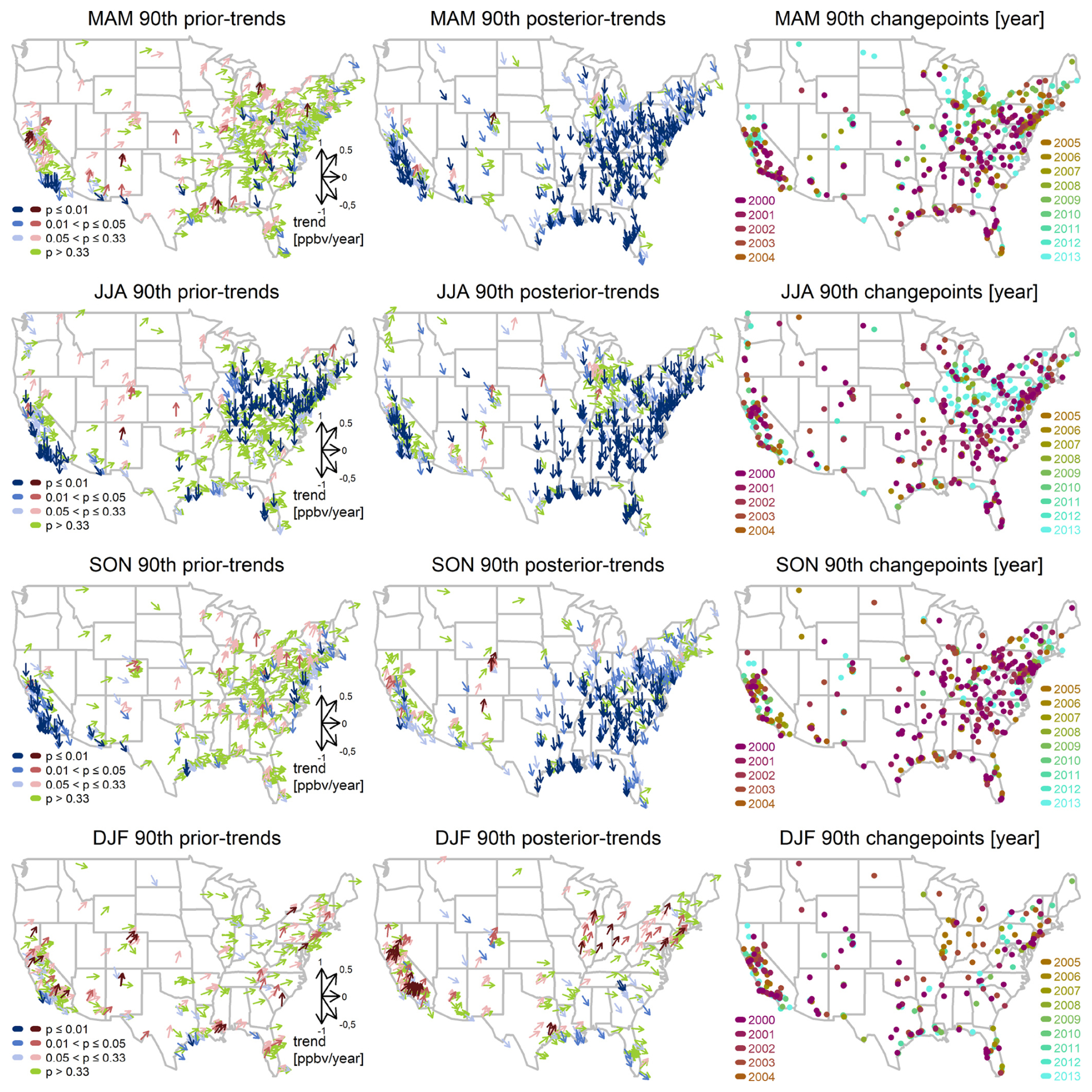
Figure 2 MDA8 trends prior (first column) and posterior (second column) to the change points (third column) for the seasonal 90th percentile over 1990–2023. For each vector, the direction indicates the trend magnitude and the color indicates its p value. The dot colors indicate the year of the change point.

For each selected site, (1) the optimized change point (identified by the greatest SNR for the trend adjustment term), (2) the trend before the change point (“prior trend”), and (3) the trend after the change point (“posterior trend”), are evaluated. Trend results are categorized by different scales, based on the thresholds of p value at 0.01, 0.05, and 0.33 (corresponding to SNR values of ± 3, ± 2, and ± 1, respectively). The overall confidence levels discussed below are assessed by the evidence and agreement of trends observed across the conterminous USA (see Appendix A for further discussions), instead of by the significance at individual stations (Mastrandrea et al., 2010); patterns recognized in the east and west or in smaller-scale regions will be pointed out specifically. We use the results for the seasonal 90th percentile to highlight the effectiveness of our approach (Fig. 2). The complete results for the seasonal 50th and 10th percentiles are provided in Figs. A3 and  A4, the percentages of posterior trends by different reliability scales are summarized in Table A2, and the percentages of trend changes based on different scenarios (e.g., from positive to negative trends, or vice versa) are summarized in Table A3. The main findings are as follows:

• For MAM, JJA, and SON, the plurality of sites show limited evidence of prior trends in the seasonal 90th percentile, except for the Northeastern USA (discussed below). Nevertheless, with different change points detected since the 2000s (as the latent periods for emission controls may vary geographically; Box and Tiao, 1975), reliable and consistent negative posterior trends can be found in MAM, JJA (high agreement and robust evidence), and SON (medium agreement and robust evidence). However, at the 50th percentile, consistency in reliable negative posterior trends can only be observed in MAM (medium agreement and robust evidence) and JJA (high agreement and robust evidence). In these cases, stronger decreasing posterior trends are found at the 90th percentile than the 50th percentile, indicating faster declines in extreme intensity. Ozone extreme percentiles not only have reliably decreasing posterior trends at the majority of sites but also have very few reliably increasing posterior trends. In MAM and JJA, less than 1 % and 3 % of sites show reliably (p≤ 0.05) positive posterior trends at the 90th and 50th percentiles, respectively. While at the 50th percentile in SON and at the 10th percentile in MAM, JJA, and SON, the plurality of sites show limited evidence of posterior trends.

• For JJA, notably, although the change points at many sites occur around the early 2000s in the eastern USA, a distinctive pattern is found across the Northeastern USA. In the latter region, the optimized change points are found around 2013 and reliable negative trends are detected over 1990–∼ 2013, while in the recent decade (∼ 2013–2023), the trends are flat and do not show further decreases. This flattened pattern might be related to the deceleration of NO_x emission reductions since 2010 (Jiang et al., 2018, 2022). The reader is referred to the next section for further discussions.

• For DJF, many stations have no measurements in wintertime, so a less dense geographical coverage is present. Medium agreement and robust evidence of increasing posterior trends can be found at the 10th percentile (41.4 %). A substantial number of sites show reliable positive posterior trends at the 90th (24.4 %) and 50th (34.6 %) percentiles, although the majority of sites show no trends (≥ 40 %). Increasing posterior trends are mainly observed in the Northeastern and the Southwestern USA.

3.2 Regional trends

While the change point detection at individual stations provides a great deal of details regarding the pattern recognition of large-scale trend changes, it is not uncommon to observe a mixture of positive and negative trends in certain subregions (e.g., mixed trends are commonly observed at the 10th percentile), which have become an obstacle to drawing generalized conclusions. Therefore, this section aims to tackle this issue by explicitly accounting for spatial heterogeneity and quantifying the overall regional trends across the eastern and western USA. Note that the trend results in Sect. 3.1 are based on selected stations where the longest records are available; however, in this section, all of the station information (including sites with a shorter or an interrupted record in Fig. 1; the same data availability criterion is applied) is used to perform geostatistical modeling and regional trend analysis.

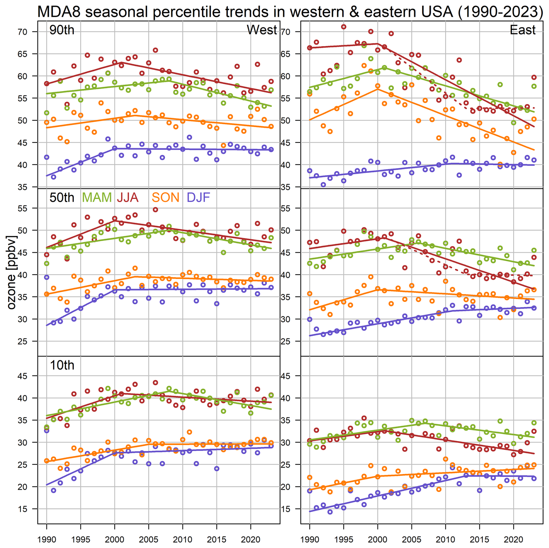
Figure 3 Regional MDA8 trends in the seasonal 90th, 50th, and 10th percentiles, based on daily MDA8 values from all available sites, in the western and eastern USA (1990–2023). For the JJA 90th and JJA 50th percentiles in the eastern USA, trends based on one change point (solid lines) or two change points (dotted lines) are shown.

Table 1 Ozone trends (± 2σ and p value), in units of parts per billion by volume per decade, at the seasonal 90th, 50th, and 10th percentiles in the western and eastern USA, including the optimized change point (CP), prior trends (1990–CP), and posterior trends (CP–2023).

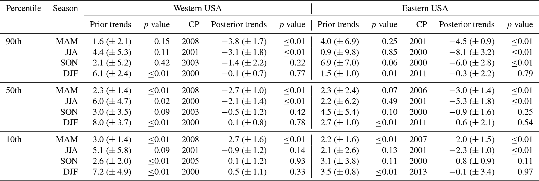
The technical evaluations of different geostatistical modeling approaches are provided in Sect. S1 in the Supplement. In summary, we find that a fast and robust estimate can be achieved by the Gaussian process approach, which is applied in the following analysis. The mapping procedure is carried out for different seasons and percentiles over the period from 1990 to 2023, and the resulting regionally aggregated time series are shown in Fig. 3 (trend values are provided in Table 1). The overall conclusion is that positive trends have been observed in MAM, JJA, and SON since 1990, although with varying turnaround points since the 2000s; these trends then turned around to be strongly and reliably decreasing (as expected from Figs. 2, A3, and A4), while flat or weak DJF trends have been observed in recent years. Specifically, the following points were found:

• This regional analysis provides effective quantifications of the overall trends. For example, a visual recognition of regional patterns in the western USA is challenging, because the trends are less consistent and spatial coverage is relatively sparse compared to the eastern USA. Nevertheless, our regional analysis shows that, albeit with weaker magnitudes in the western USA, seasonal posterior trends at different percentiles generally follow the same conclusions between the eastern and western USA.

• In MAM, JJA, and SON, the 90th percentile has strong and reliable negative posterior trends, except for the western USA in SON. The results also show that the lower the percentiles, the weaker the magnitude of the negative trends. Controls on ozone precursor emissions in the USA have been designed to reduce extreme ozone levels, and our observation that the strongest negative trends occur at the 90th percentile is consistent with those efforts.

• The strongest negative seasonal trend in this regional assessment was found in the eastern USA, at the JJA 90th percentile (−8.1 (± 3.2) ppbv per decade, p≤ 0.01), followed by the SON 90th percentile (−6.0 (± 2.8) ppbv per decade, p≤ 0.01), the JJA 50th percentile (−5.3 (± 1.8) ppbv per decade, p≤ 0.01), and the MAM 90th percentile (−4.5 (± 0.9) ppbv per decade, p≤ 0.01).

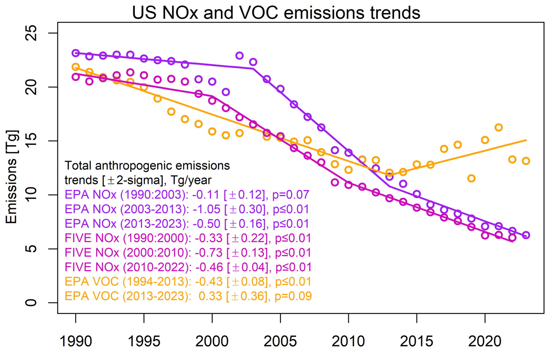
Figure 4 Annual US NO_x and VOC trends: estimates include EPA national air pollutant emissions trends for NO_x (purple) and VOCs (orange). In addition, the FIVE NO_x (magenta) emissions are based on the EPA estimates, but the mobile emissions from “highway vehicles” and “off-highway categories” were replaced with the estimates from the Fuel-Based Inventory for Vehicle Emissions (FIVE) (Harkins et al., 2021).

• As discussed in Sect. 2, we mainly consider one unknown change point for long-term trends over the 34-year period. However, previous satellite observations have shown that US NO_x emissions did not decline until the late 1990s (McDonald et al., 2012), and the pace has likely decelerated since 2010 (Jiang et al., 2018, 2022), as primarily found in rural areas (Silvern et al., 2019; Christiansen et al., 2024). Alternatively, the EPA's national air pollutant emission trend dataset can be used to study total anthropogenic NO_x and VOC (volatile organic compound) emissions (US EPA, 2024b). In addition, the Fuel-Based Inventory for Vehicle Emissions (FIVE) provides improved NO_x estimates of mobile emissions (McDonald et al., 2014, 2018; Harkins et al., 2021). FIVE can be used to replace the estimates from “highway vehicles” and “off-highway categories” in the EPA dataset, to produce an updated total anthropogenic NO_x emissions inventory. Based on the same change point analysis (Fig. 4), the following three findings are observed. First, reliably negative VOC trends (p≤ 0.01) were found between 1990 and 2013, but these trends became positive after 2013 (p = 0.09). Second although the EPA NO_x trends show a reduction in the late 1990s, the first change point is identified in 2003, due to a spike in 2002, followed by a rapid decline (p≤ 0.01) over the period from 2003 to 2013. The decreasing trends weakened after 2013, although still with high confidence (p≤ 0.01). Third, similar to the EPA NO_x trends, the FIVE NO_x decreased from 1990 to 2022, with an acceleration at 2000 and a deceleration at 2010, which occurred 3 years earlier than the change points in the EPA NO_x trends.

  Therefore, it is possible to consider an additional peripheral change point if the junctures occur separately at around 2000 and after 2010, as each trend segment satisfies a benchmark of at least 10 years in length (i.e., these changes are not likely due to short-term variability). We identify two cases that fit this scenario, which are the 90th and 50th percentiles in JJA in the eastern USA (the other cases are so variable that the second change point is generally unnecessary or premature). We fit the trends with two change points for these two time series (dotted lines in Fig. 3) and find the second change point aligned with the flattened ozone after 2013. These two change points appear to explain two distinct site patterns of JJA trends in the Eastern USA in Fig. 2: the plurality of sites capture the emission reductions around 2000 (the primary change), and some sites coincide with flattened ozone trends after 2013 (the secondary change). As Fig. 2 already identified which sites have a change point around 2013, it seems unnecessary to conduct a duplicate analysis by considering two-change-point modeling for individual sites, given that this particular analysis is reasonable partly due to the regional assessment providing a more clear signal.

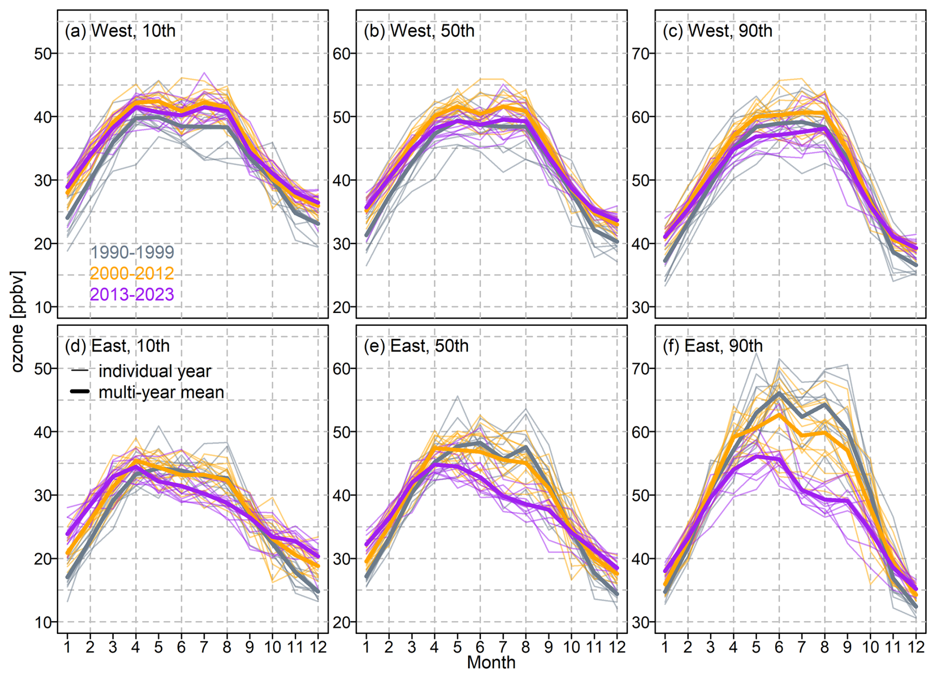
Figure 5 Regional MDA8 monthly percentiles over different years (thin lines) and periods (bold lines) in the western and eastern USA (1990–2023).

• Strong heterogeneity in seasonal trends across the eastern USA substantially changes the ozone seasonality. We compare the regional monthly percentiles over different periods in Fig. 5, based on the same geostatistical modeling approach and based on individual year and multiyear averages. We can clearly see that the seasonal peaks at the 90th and 50th percentiles shifted from summer in 1990–1999 to spring in 2013–2023 (this period is chosen because JJA ozone tends to be steady over 2013–2022), along with increased ozone in DJF and decreased ozone in other seasons. In the western USA, the shape of the seasonal cycles remains similar, although the 90th percentile clearly decreased from 2000–2012 to 2013–2023 during MAM and JJA. A modeling study by Clifton et al. (2014) showed that, under continued emission controls, surface ozone seasonal peaks are expected to shift to February–March by the end of the 21st century over the Northeastern USA; the current peak in April suggests that the observed seasonal cycle might follow the model prediction by Clifton et al. (2014), but a modeling study is necessary to confirm the detailed process.

• For the 6-month warm season (April–September), a previous regional trend study found an overall mean MDA8 trend of −0.43 (± 0.28) ppbv yr⁻¹ (p≤ 0.01) in eastern North America over 2000–2014 (Chang et al., 2017). Albeit with a different domain, a trend value of −0.39 (± 0.16) ppbv yr⁻¹ (p≤ 0.01) is found in the eastern USA over the period from 2000 to 2023. The corresponding trend in the western USA is −0.16 (± 0.10) ppbv yr⁻¹ (p≤ 0.01).

This analysis summarizes the current status of consistent decreases in ozone extremes at the regional scale. While the reductions are apparent and profound, some abnormally high ozone levels can be observed in recent years (e.g., 2018 and 2021 in the west and 2023 in the east), as also indicated by the spatially interpolated maps of the 90th percentile in JJA (Fig. S3), which can be associated with extensive wildfires seasons and/or heat waves (Bartusek et al., 2022; Langford et al., 2023; Rickly et al., 2023; Cooper et al., 2024). As wildfires and heat waves are expected to continue to increase, they will likely impact surface ozone levels across the USA in the near future (see the next section for further discussions).

4 Results: potential ozone climate penalty due to heat waves

In the previous section, we concluded that strong reductions in regional surface ozone extremes occurred across much of the USA over the past 2 decades. In this section, we aim to investigate potential short-term and long-term impacts of heat wave events on ozone exceedances. As we expect to classify a majority of data into normal days and a minority of data into heat wave days, a comparison based on the extreme percentiles might not be feasible due to fewer samples during heat wave events; therefore, the probability of threshold exceedances is used in the analysis.

This analysis is focused on the period from 1995 to 2022 for three reasons. First, this period is a balance between an inclusion of more sites (more than 25 years in Fig. 1) and a sufficiently long period (nearly 30 years). Second, ozone exceedances have consistently decreased in this period (Sect. 4.1), so we can investigate if heat wave events halt the progress of emission controls. The possible deceleration of emission trends should not play an important role here, as its influence is expected to be similar between heat wave and normal conditions. Third, 2023 is an anomalous year with many ozone exceedances across the Upper Midwest and the Northeastern USA due to large forest fire plumes transported from Canada (Cooper et al., 2024). These large numbers of exceedances are not observed in the previous decade (2013–2022). Therefore, the 2023 data are excluded to avoid skewing our trend estimates.

The distribution and trends in ozone exceedances based on all daily MDA8 ozone values during May–September are provided in Appendix B (without distinguishing normal and heat wave conditions). This section first investigates the short-term heat wave impact on ozone and then compares long-term ozone exceedances between heat wave and normal days.

4.1 Heat wave metrics and short-term impact on ozone

To gain a quick insight into the temperature variability, we assess trends in T_max and T_min (Fig. S5) and the trends in heat wave frequency (the number of heat wave days per May–September) based on different heat wave metrics (Fig. S6). Despite certain clusters of positive trends being detected, inconsistent spatial patterns of trends are observed between T_max/T_min and different heat wave metrics. It is, thus, important to acknowledge that temperature trends are also heterogeneous, so their assessed impact on ozone should not be based solely on a single heat wave metric. Nevertheless, by using generalized additive modeling methodology and interpolating gridded daily temperature data onto all ozone monitoring sites, we find substantially stronger correlations between MDA8 and T_max than MDA8 and T_min (Fig. S7). Therefore, we only consider heat wave metrics based on T_max hereafter.

It should be noted that the analysis results in Appendix B are based on all available long-term sites over the period from 1995 to 2022; however, the higher the temperature thresholds, the fewer the number of sites that qualify (e.g., extreme temperatures are present but have not occurred consecutively). To ensure that a site has enough data for accurate trend detection, we only show the results when heat waves occurred in at least 10 years between 1995 and 2022. The implication is that, as a large portion of sites have insufficient records that meet the TX35deg metric, the TX35deg results are merely provided for a reference, and the main conclusions are based on the TX90pct and TX95pct metrics.

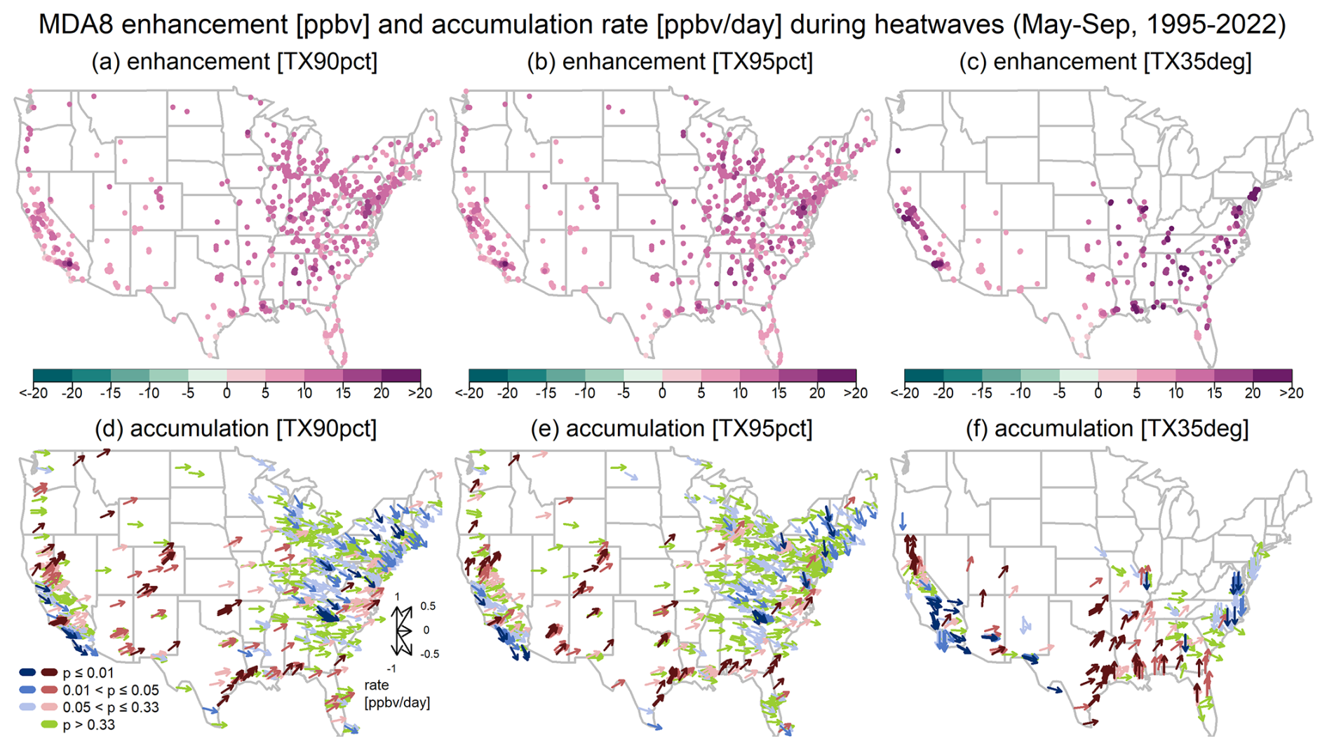
Figure 6 MDA8 average differences between heat wave and normal conditions (enhancement, a–c) and the rate of daily ozone changes when heat waves events continue and extend (accumulation, d–f), based on various heat wave metrics (May–September, 1995–2022).

The results for short-term ozone statistics based on different heat wave metrics are shown in Fig. 6. Positive ozone enhancements can be observed consistently across most locations, with an overall average enhancement (standard deviation, or SD) of 5.9 (SD = 2.9) ppbv, 6.3 (SD = 3.2) ppbv, and 9.9 (SD = 6.2) ppbv (the latter is subject to fewer sites) for the TX90pct, TX95pct, and TX35deg metrics, respectively. Although a large portion of sites show no evidence (p> 0.33) of ozone accumulation (Table S1 in the Supplement), we find that around 30 % of sites in the western USA have reliable positive accumulation values (p≤ 0.05), based on the TX90pct and TX95pct metrics. For the eastern USA, reliable positive accumulation values only occurred at around 10 % of sites, and these are mainly observed in the Southeastern USA. Both eastern and western USA have around 10 % of sites with reliably decreasing ozone accumulation (p≤ 0.05). In summary, ozone deterioration during heat wave events can be generally anticipated across the western and southern USA.

4.2 Ozone exceedances under heat wave and normal conditions

In this section, we investigate if the long-term trends in ozone exceedances exhibit any different patterns when the analysis is constrained to heat wave observations (by partitioning the time series into two mutually exclusive sets: heat wave and normal days). The aims of this analysis are to (1) quantify the differences in exceedance probability (EP) values between heat wave and normal conditions and (2) evaluate if the effectiveness of emission controls can be hampered during heat wave events.

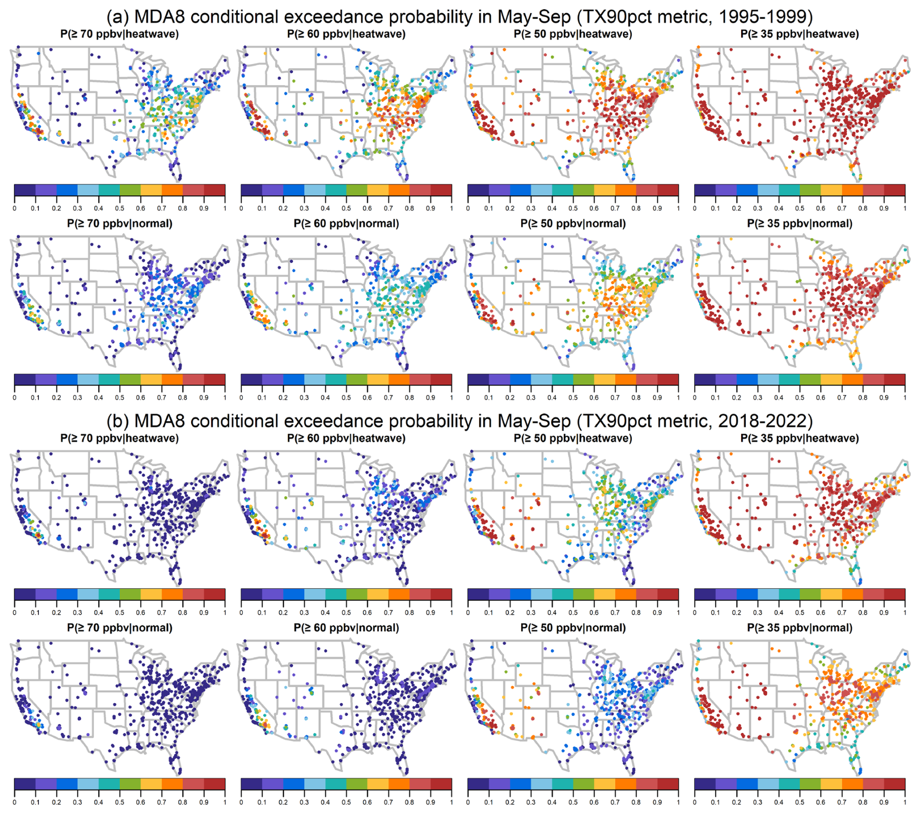
Figure 7 Conditional probabilities of MDA8 exceedances in May–September, based on various ozone thresholds, and the average over (a) 1995–1999 and (b) 2018–2022.

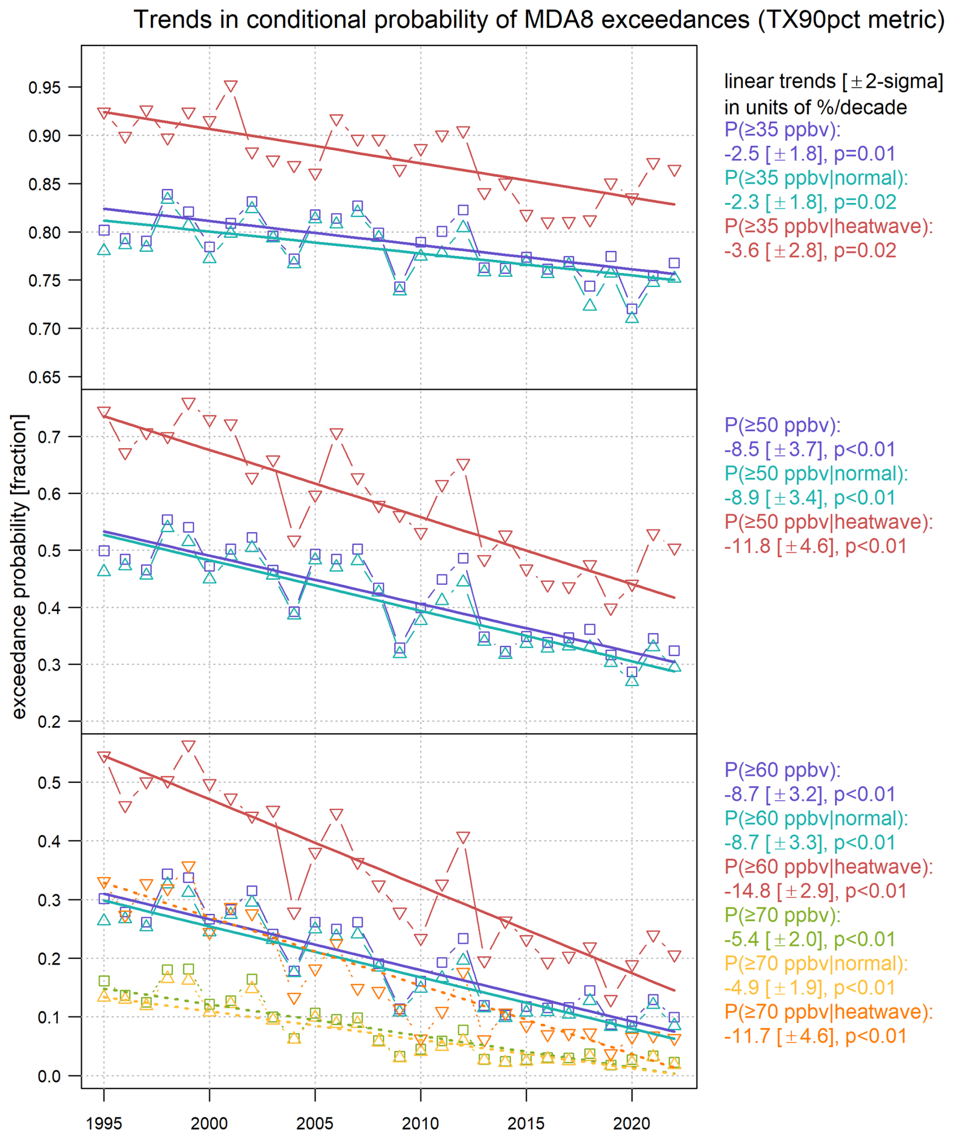
Figure 8 Summary of trends in unconditional and conditional exceedance probabilities, based on various ozone thresholds and the TX90pct metric (May–September, 1995–2022). Squares indicate unconditional probabilities. Upward and downward triangles indicate conditional probabilities for normal and heat wave days, respectively.

Similar to the unconditional probability (P_E) in Fig. B1, we show the EPs conditioned on heat wave and normal days based on the TX90pct metric in Fig. 7 (denoted by P_E|H and $P_{E|\stackrel{\mathrm{‾}}{H}}$, respectively). Similar patterns between P_E and $P_{E|\stackrel{\mathrm{‾}}{H}}$ can be observed for different thresholds and periods. As expected, P_E|H is generally greater than $P_{E|\stackrel{\mathrm{‾}}{H}}$ at different thresholds, and it also clearly decreased between 1995–1999 and 2018–2022. The above results also hold for the TX95pct and TX35deg metrics (Figs. S8 and S9). To give an overall comparison and summary of Figs. B2 and 7, we calculate the annual May–September averages of P_E, P_E|H, and $P_{E|\stackrel{\mathrm{‾}}{H}}$ across all long-term sites (using a simple average, no weighting is applied) and estimate the trends in Fig. 8. In terms of probability theory, if $P_{E|H}>P_{\mathrm{E}}$, it implies that ozone exceedances and heat waves are positively correlated (see Sect. S2). Nevertheless, the difference between P_E|H and $P_{E|\stackrel{\mathrm{‾}}{H}}$ provides a more clear indication about the magnitude of enhanced EPs during heat waves. The findings can be summarized as follows:

• For the threshold of 70 ppbv, the baseline EP ($P_{E|\stackrel{\mathrm{‾}}{H}}$) is around 17 % in the early period and 3 % since 2013, with a trend of −4.9 (± 1.9) % per decade. P_E|H is substantially greater than $P_{E|\stackrel{\mathrm{‾}}{H}}$ in the early period, but the differences are reduced from 18 % in 1995–1999 to 4 % in 2018–2022.

• For the thresholds of 60 and 50 ppbv, heat waves increase the EP by 16 % and 18 % on average (p≤ 0.01, based on paired t test), respectively, but the differences are reducing over time because P_E|H shows stronger decreasing trends than $P_{E|\stackrel{\mathrm{‾}}{H}}$.

• Note that because the baseline EP for 35 ppbv (typically more than 70 % of days in May–September) is much higher than 50 and 60 ppbv under normal conditions, naturally it restricts the room for additional enhanced EPs during heat waves (bounded by 1). We find that heat waves increase the EP by 10 % on average (p≤ 0.01) for the threshold of 35 ppbv, and we do not find evidence that their differences have changed over time.

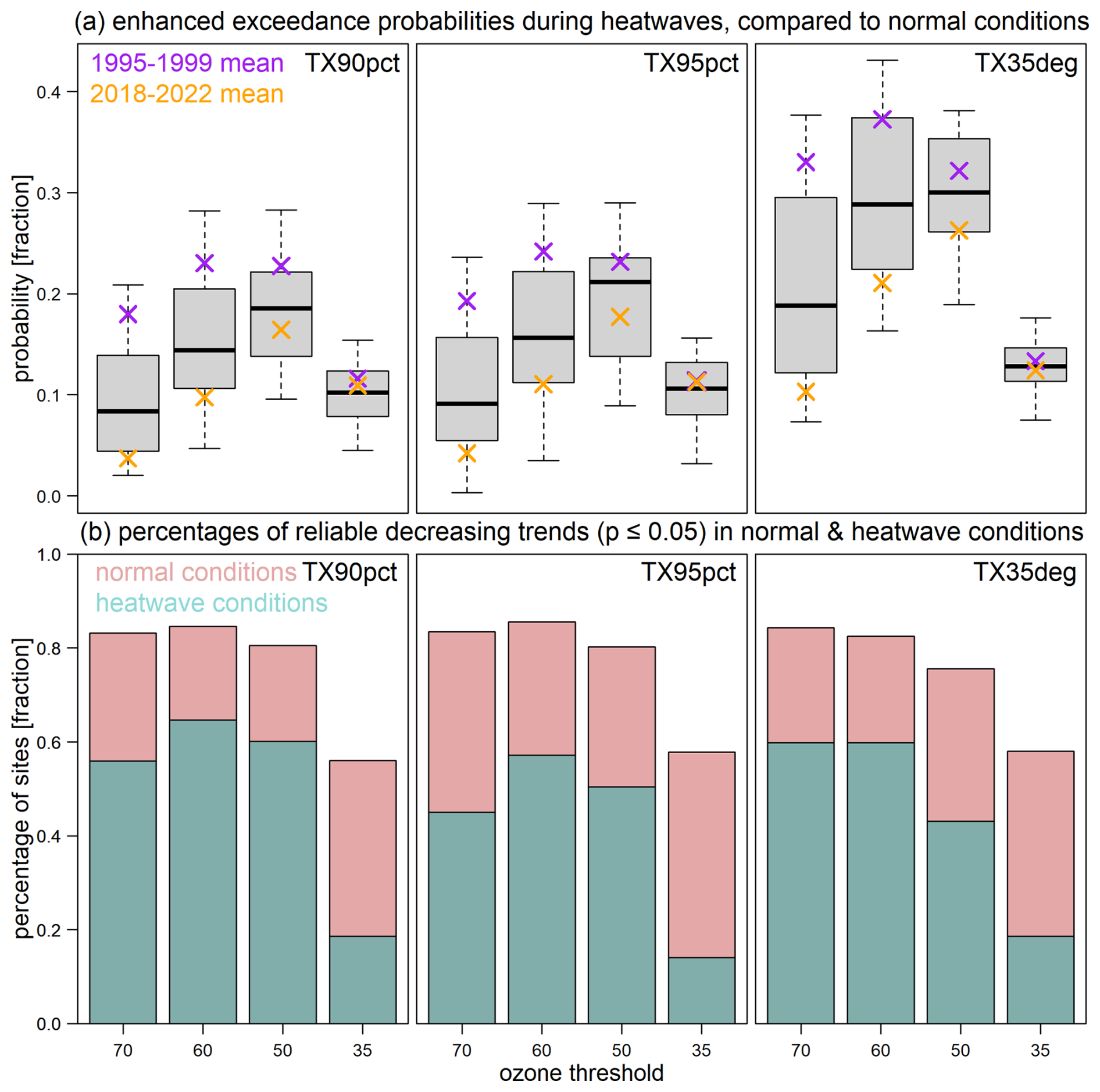
Figure 9 Summary of (a) enhanced exceedance probabilities (each bar is comprised of 28 estimates of $P_{E|H}-P_{E|\stackrel{\mathrm{‾}}{H}}$ over 1995–2022; averages over 1995–1999 and 2018–2022 are shown using purple and orange crosses, respectively) and (b) the percentages of reliable decreasing exceedance trends (p≤ 0.05) under normal and heat wave conditions, based on various ozone thresholds and heat wave metrics (May–September, 1995–2022).

We show the distribution of the enhanced EPs (annual estimates of $P_{E|H}-P_{E|\stackrel{\mathrm{‾}}{H}}$ over 1995–2022) under different heat wave metrics in Fig. 9a. Overall, similar conclusions can be drawn for the TX95pct and TX35deg metrics (also see Figs. S10 and S11).

The major limitation of the above analysis is that heat wave trends and variability are not taken into account. This technical challenge is because P_E|H is undefined when P_H=0, implying that P_E|H can only be calculated when a heat wave has already occurred. Therefore, the above analysis does not reflect the reality that heat wave events may be fewer in the early period and more frequent in the present day. In order to account for the heat wave variability, we estimate exceedance trends at individual sites based on the logistic regression, which also allows P_H=0 in certain years. The hypothesis is that because heat waves have become more frequent, they are likely to contribute to additional ozone exceedances, slowing the progress of decreasing the frequency of ozone exceedances. By comparing the exceedance trends under normal and heat wave conditions, we are able to quantify how many reliable decreasing exceedance trends are sustainable under heat wave conditions. The results are summarized in Fig. 9b: we find that reliable decreasing exceedance trends cannot be maintained for around 20 %–30 % of sites at the thresholds of 70, 60, and 50 ppbv or for around 40 % of sites at the threshold of 35 ppbv. A more detailed view of exceedance trends under normal and heat wave conditions is provided in Figs. S12–S14 (and discussed in Sect. S3). In summary, these findings imply that heat wave events not only increase the EP but also likely slow down the decreasing exceedances by its increasing frequency.

Although the TX90pct metric is previously recommended to study heat waves (Perkins and Alexander, 2013), this metric might not necessarily be ideal for correlating heat waves with ozone. The advantages of the TX90pct are that its threshold is tailored to different environments, and it thus ensures sufficient heat wave observations. However, the 90th percentile might not represent the extreme temperature condition, especially for middle and high latitudes. Our findings show that a higher temperature threshold results in fewer reliably negative exceedance trends and fewer data that meet the heat wave condition. Therefore, the results are subject to the limitation of fewer samples being used for trend detection in heat wave conditions. As a longer time period makes the estimation of higher temperature thresholds more reliable, future studies are recommended to use multiple heat wave thresholds to quantify the heat wave impact on ozone.

For our final analysis, we identify the monitoring sites that have experienced a clear ozone climate penalty over the relatively short time period of 1995–2022. We derived trends in co-occurrences (P_E∩H) based on different ozone thresholds and heat wave metrics (Fig. S15) and found that positive P_E∩H trends (p≤ 0.05) can be commonly observed on the West Coast of the United States. However, we do not find similar evidence that the correlations between ozone exceedances and heat waves have increased (Fig. S16). The reason behind this is that the correlations are jointly determined by P_E∩H, P_E, and P_H; thus, trends in correlations can be counterbalanced by stronger decreasing P_E and weaker increasing P_H and P_E∩H. This result is consistent with a recent study which shows that emission controls reduce the summertime ozone–temperature sensitivity (Li et al., 2025). Therefore, positive trends in co-occurrences do not necessarily lead to increasing correlations between ozone exceedances and heat waves.

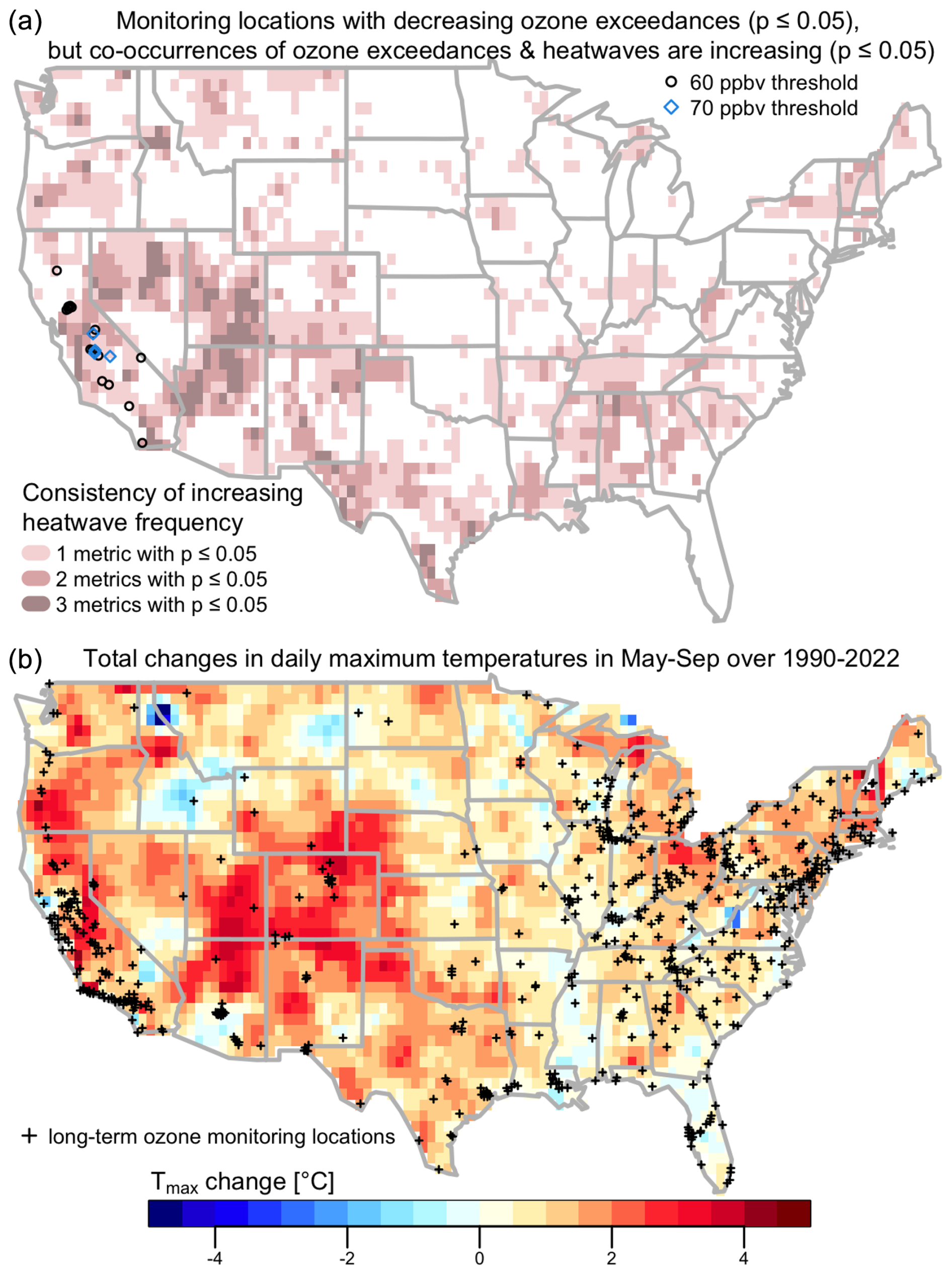
Figure 10 Panel (a) shows ozone monitoring locations with a clear indication of climate penalty: selected sites show decreasing ozone exceedances above 70 and/or 60 ppbv (p≤ 0.05), but increasing trends in co-occurrences of ozone exceedances and heat waves are detected (p≤ 0.05) based on at least two out of three heat wave metrics. The background indicates increasing heat wave trends (p≤ 0.05) detected by one (pink), two (red), or three (brown) heat wave metrics. Panel (b) shows estimated increases in the daily maximum temperatures in May–September over 1990–2022. Black crosses indicate long-term monitoring locations used in the heat wave analysis.

To identify the locations with a clear climate penalty, we searched for the monitoring sites that show decreasing ozone exceedances (p≤ 0.05) but have increasing co-occurrences of exceedances and heat waves (p≤ 0.05) over the same period (Fig. 10). In this map, we used 70 or 60 ppbv as the ozone threshold, and all three heat wave metrics were considered, but we only showed the results when at least two out of three heat wave metrics revealed a likely climate penalty. We identified 19 sites that have experienced a climate penalty since 1995. Co-occurrence time series of 70 ppbv threshold exceedances and heat waves are shown at four of these locations (Fig. S17). All of these sites are in California and are associated with daily maximum temperature increases of 1–3 °C over the 3 decades from 1990 to 2022 (May–September only) (Fig. 10). Many states in the western USA have regions with similar or greater temperature increases, but we did not find evidence of a climate penalty. However, our study is limited by the fact that ozone monitoring is sparse in many of these regions and, therefore, the climate penalty cannot be thoroughly evaluated.

5 Conclusions

Previous studies on US surface ozone observations have shown a substantial reduction in warm-season ozone across much of the USA since the early 2000s, in response to strict controls on anthropogenic emissions (Cooper et al., 2012; Simon et al., 2015; Strode et al., 2015; Lin et al., 2017; Jin et al., 2020; Seltzer et al., 2020; Simon et al., 2024). However, several outstanding issues are noted, including (1) oil and gas emissions (McDuffie et al., 2016; Francoeur et al., 2021), which can contribute to wintertime ozone exceedances in the Uinta Basin, Utah (Edwards et al., 2014); (2) wildfire influence, which has been associated with regional-scale ozone exceedances in recent years (Langford et al., 2023; Byrne et al., 2024; Cooper et al., 2024); and (3) heat waves, which provide ideal conditions for ozone production (Schnell and Prather, 2017). By quantifying trends based on all available MDA8 ozone observations over the extended period from 1990 to 2023, we found that our analysis is consistent with prior studies, but we have been able to update trends to the present day; moreover, for the first time, we provide observational evidence of the ozone climate penalty in regions with large temperature increases and widespread ozone monitoring.

Incorporating change point(s) in the trend detection model is also known as an intervention analysis in statistics (Box and Tiao, 1975), as it enables us to quantify the effectiveness of an intervention (e.g., anthropogenic emissions control). By focusing on the results after the change points, our findings can be summarized as follows:

• Based on individual long-term sites (1990–2023), we find that at least 46 % of sites have reliably negative trends and at most 3 % of sites have reliably positive trends at the 90th seasonal percentile in MAM, JJA, and SON and at the 50th percentile in JJA (medium to high agreement). In contrast, reliably positive DJF trends are observed more commonly at the lower percentiles (41 % at the 10th percentile versus 35 % at the 50th percentile and 24 % at the 90th percentile), albeit subject to lower site availability than other seasons.

• Based on regional geostatistical modeling, we found that the higher the percentiles, the stronger the negative regional trends in MAM, JJA, and SON. Robust negative trends (p≤ 0.01) can be identified in MAM and JJA at the 50th and 90th percentiles in both the western and eastern USA, while in SON robust negative trends can only be found at the 90th percentile in the east.

• In response to the shift in satellite NO_x emission trends from a rapid decline since the late 1990s to a slowdown after 2010 (McDonald et al., 2012; Jiang et al., 2018, 2022), we explored the possibility of incorporating two change points for trend detection. We found that this shift fits the summer ozone variability in the Eastern USA (the 90th and 50th percentiles). The primary change point around 2000 corresponds to substantial ozone decreases and the secondary change point at 2013 corresponds to flattened ozone trends (Fig. 3). This pattern is currently not identified in other seasons and percentiles. Recent studies have also shown that the slowdown in NO_x trends is mainly found over rural areas, while NO_x has continued to decrease in urban areas (Silvern et al., 2019; Christiansen et al., 2024). The impact of the most recent NO_x trends might take additional years to become apparent and attributable to ozone variability, and this warrants future modeling studies.

In the eastern USA, despite the fact that flattened JJA trends are observed after 2013, the added value of our long-term study is to show that the rapidly declining JJA trends in the 2000s substantially reshaped the regional ozone season, with the seasonal peak shifting from summer in the 1990s to spring in the most recent decade.

To deliver an observational-based assessment of the heat wave impact on ozone extremes, we compare MDA8 exceedance probabilities and trends based on different heat wave metrics. In summary, the effectiveness of emission controls leads to substantial reductions in exceedances above 70, 60, and 50 ppbv. Although the exceedance probabilities are typically higher during heat waves than under normal conditions, the differences are substantially reduced in the present-day period (2018–2022). We also find that reliable decreasing exceedance trends are likely to have halted at 20 %–40 % of sites during heat waves, dependent on the ozone thresholds and heat wave metrics. Therefore, heat waves not only increase the exceedance probabilities but also likely slow down the effectiveness of emission controls. The limited number of sites that have experienced a clear ozone climate penalty since 1995 are all located in California, where the ozone monitoring network is dense. The sparse ozone monitoring network across the other regions of the western USA, where temperatures have increased greatly, hinders our ability to identify other locations that may have experienced a climate penalty. This climate penalty analysis is also limited because the available ozone time series are less than 30 years in length, while the chemistry–climate model projections for identifying regions most likely to experience an ozone climate penalty are based on much longer timescales (Zanis et al., 2022). Apart from heat waves, recent studies also show that the increasing occurrence of wildfires could be an important factor for ozone exceedances in the present-day and near future (Langford et al., 2023; WMO, 2023; Cooper et al., 2024; Seguel et al., 2024).

Appendix A: Further discussions and additional results for seasonal percentile change point analysis

In Sect. 3.1, our focus has been on the seasonal extreme percentile. This section aims to provide more detailed discussions on the confidence levels for a trend assessment and on the analysis for additional percentiles (Figs. A1 and A2). In the main text, we applied geostatistical modeling techniques to summarize the regional trends (Sect. 3.2). An alternative approach can be used based on the evidence and agreement obtained from individual sites. Although the method and terminology are based on Mastrandrea et al. (2010), the implementation details need to be tailored to our study (Table A1):

• Evidence. The reliability of trend estimate is classified into five scales, including robust (positive and negative trends with p≤ 0.05), medium (positive and negative trends with 0.05 < p≤ 0.33), and limited (trends with p> 0.33) evidence.

• Agreement. Long-term sites are classified according to their trend evidence. The consistency is determined by which scale has the highest percentage of sites, and it is ranked from high (> 50 % of sites are classified as the same scale), to medium (33 %–50 % of sites), to low (< 33 % of sites).

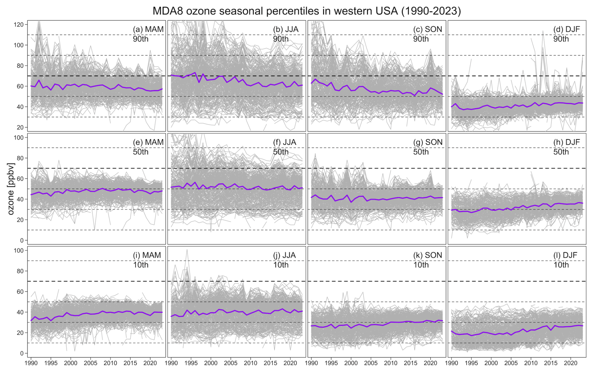
Figure A1 Ozone time series at the seasonal 90th, 50th, and 10th percentiles in the western USA: observations from individual stations are shown in gray, and simple averages are shown in purple.

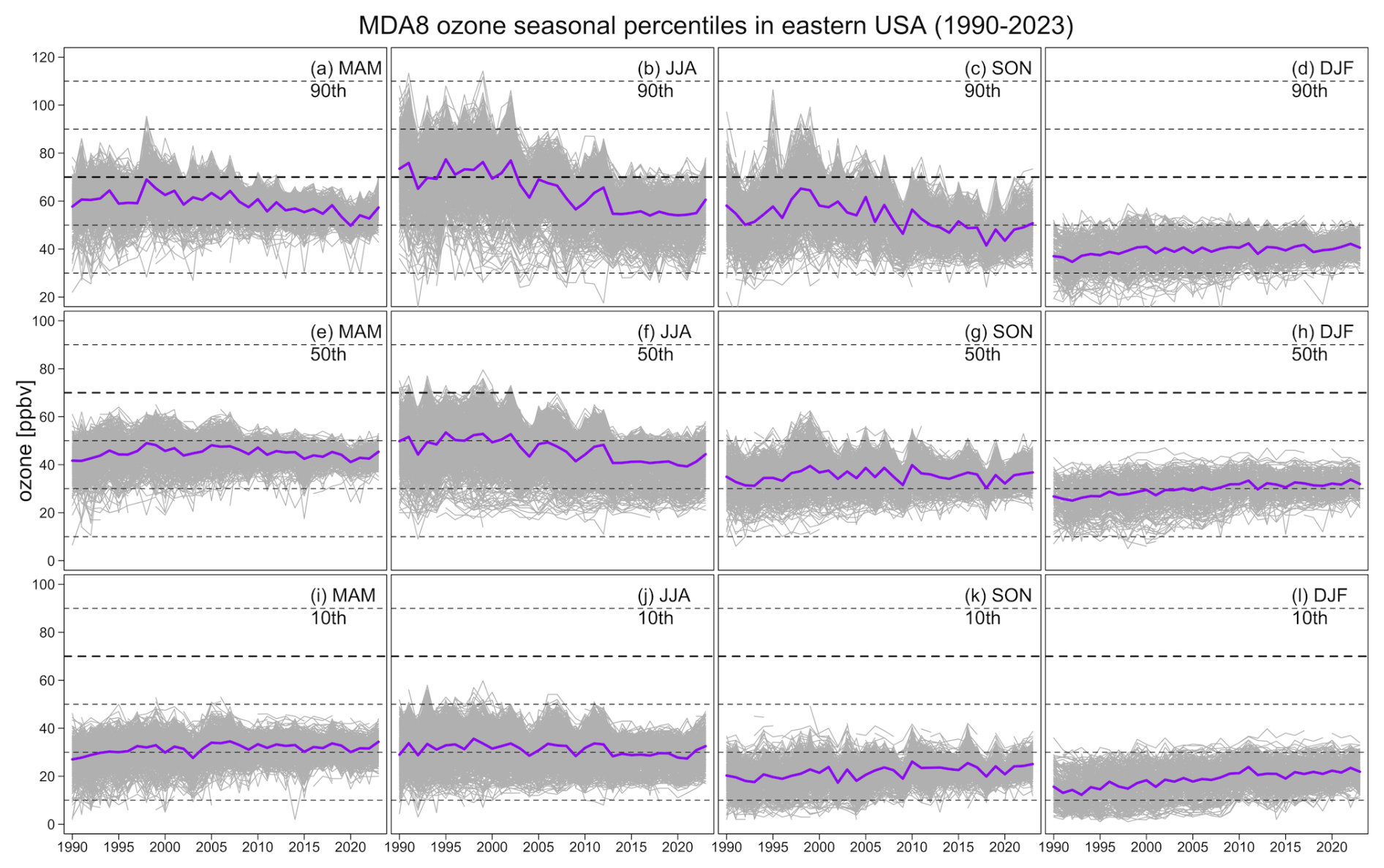
Figure A2 Ozone time series at the seasonal 90th, 50th, and 10th percentiles in the eastern USA: observations from individual stations are shown in gray, and simple averages are shown in purple.

Table A1 Criteria to determine agreement and evidence. The level of agreement is determined by which trend evidence scale has the highest percentage of sites.

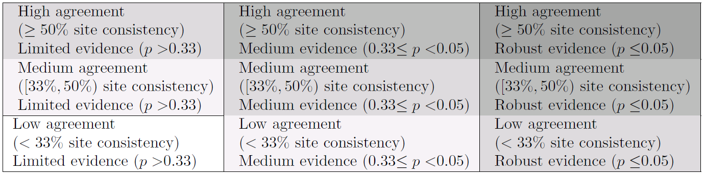
Table A2 Site percentages of posterior trends by different reliability scales in Figs. 2, A3, and A4 (trends with p≤ 0.01 are merged into p≤ 0.05). A total of 450, 462, 406, and 263 sites are available for MAM, JJA, SON, and DJF, respectively, but the relative percentages are shown for each row (i.e., sum to 100 %).

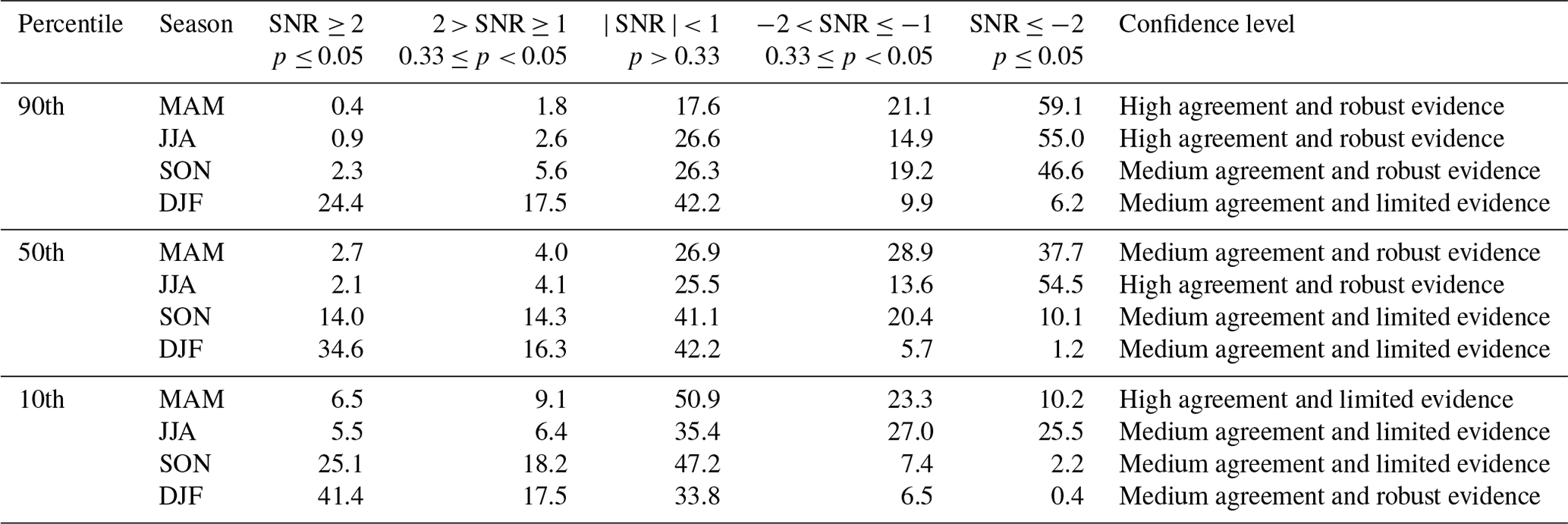
Table A3 Same format as Table A2, but the following before and after scenarios are categorized: (A) P  →  N – from reliable positive (p≤ 0.05) to reliable negative (p≤ 0.05) trends; (B) W → N – from weak (p> 0.05) to reliable negative (p≤ 0.05) trends; (C) N → P – from reliable negative (p≤ 0.05) to reliable positive (p≤ 0.05) trends; (D) W → P – from weak (p> 0.05) to reliable positive (p≤ 0.05) trends; (E) P → W – from reliable positive (p≤ 0.05) to weak (p> 0.05) trends; and (F) N → W – from reliable negative (p≤ 0.05) to weak (p> 0.05) trends. All the other scenarios (e.g., the same reliability scale before and after the change point or transitions between weak positive and weak negative) are considered to be no evidence of trend changes.

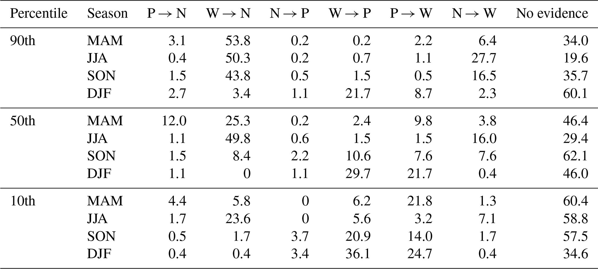
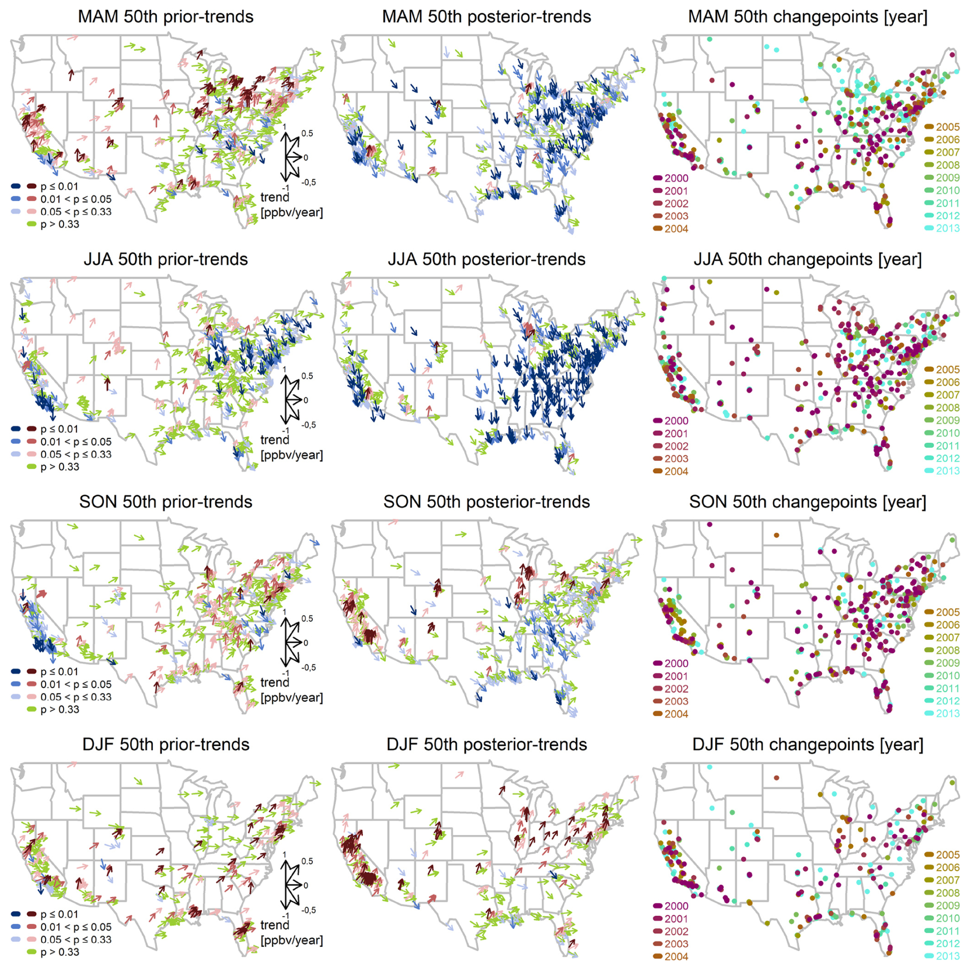
Figure A3 Same as Fig. 2 but for the seasonal 50th percentile.

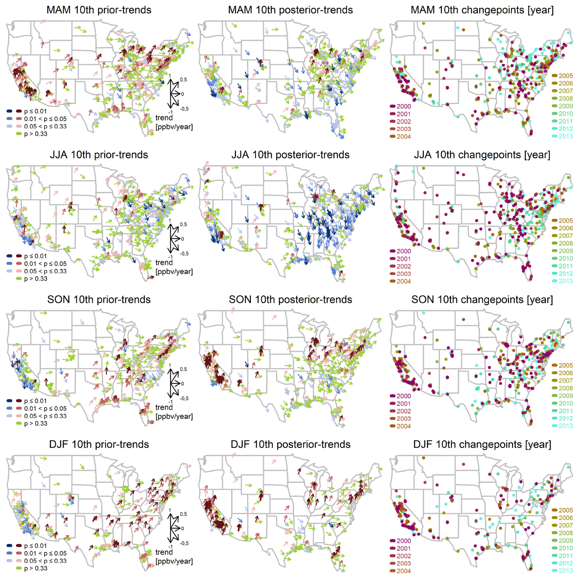
Figure A4 Same as Fig. 2 but for the seasonal 10th percentile.

This table is used to assign the confidence level to the trend assessment of individual long-term sites (Table A2; Figs. 2, A3, and A4). As geostatistical modeling techniques are more effective to explicitly quantify the regional trends, we do not further separate the western or eastern USA in Table A2. In addition, instead of using the p value to determine the reliability of the change point, a more scientifically meaningful approach is to categorize different scenarios of trend alterations before and after the change point. We consider trend alterations based on the following scenarios (Table A3):

• A

  P → N: from reliable positive (p≤ 0.05) to reliable negative (p≤ 0.05) trends;

• B

  W → N: from weak (p> 0.05) to reliable negative (p≤ 0.05) trends;

• C

  N → P: from reliable negative (p≤ 0.05) to reliable positive (p≤ 0.05) trends;

• D

  W → P: from weak (p> 0.05) to reliable positive (p≤ 0.05) trends;

• E

  P → W: from reliable positive (p≤ 0.05) to weak (p> 0.05) trends;

• F

  N → W: from reliable negative (p≤ 0.05) to weak (p> 0.05) trends.

All the other scenarios (e.g., the same evidence scale before and after the change point, or transitions between weak positive and weak negative) are considered to be no evidence of trend changes. With this approach, the results show that the plurality of sites are classified as (1) no evidence in DJF and scenario B in other seasons for the 90th percentile, (2) scenario B in JJA and no evidence in other seasons for the 50th percentile, and (3) scenario D in DJF and no evidence in other seasons for the 10th percentile. The above method to determine level of agreement can also be applied here (not shown).

Appendix B: Distribution and trends in ozone exceedances

To give an overview of the current distribution of ozone exceedances, Fig. B1 shows the average exceedance days and probabilities (P_E in Eq. 3) in May–September across the conterminous USA, based on the thresholds of 70, 60, 50, and 35 ppbv and the periods 1995–1999 and 2018–2022 (multiyear averages are taken to ensure representativeness). Exceedance days above 70 ppbv in the eastern USA in the early period have greatly diminished in the recent period. Southern California is the only cluster where greater than 30 ozone exceedance days per year are found at multiple sites in the present-day period (2018–2022). The reductions in ozone above 60 and 50 ppbv in the eastern USA are also obvious. Changes in the pattern of exceedances above 35 ppbv are less profound, but a general reduction can be observed in the eastern USA. Broadly speaking, for the threshold of 50 or 35 ppbv, the number of exceedances across the Southwestern USA has remained relatively constant (except along the California coast).

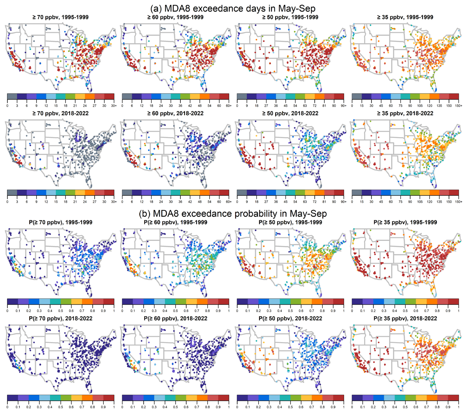
Figure B1 MDA8 exceedance days (a) and probabilities (b) based on various ozone thresholds in the early period (1995–1999) and present day (2018–2022).

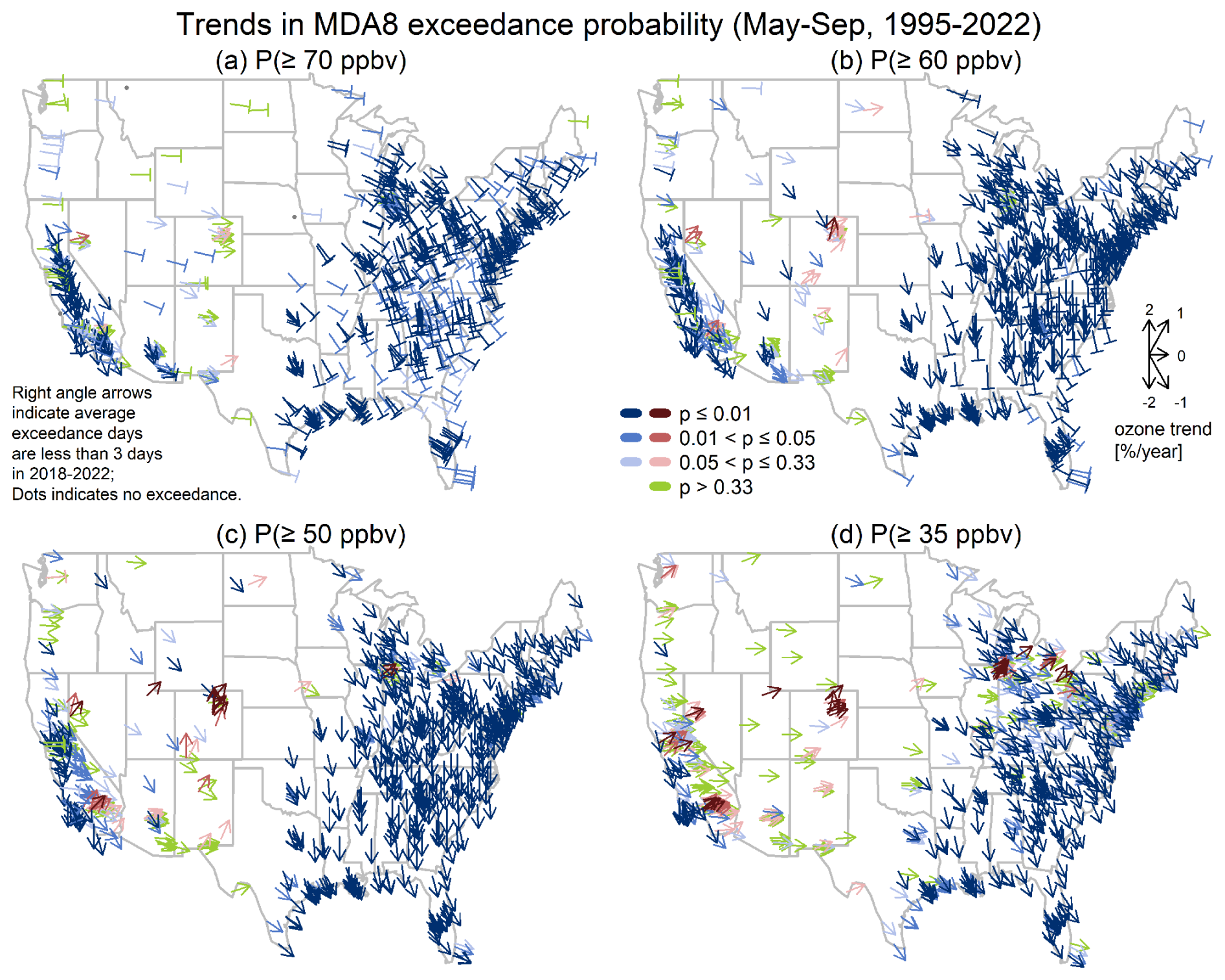
Figure B2 Trends (% yr⁻¹) in MDA8 exceedance probabilities based on various ozone thresholds (May–September, 1995–2022).

We further show the trends in ozone exceedances over 1995–2022 in Fig. B2, based on the probability measure (a change rate of 1 % yr⁻¹ corresponds to 1.53 d yr⁻¹, given that the total number of days is constant in May–September). As expected, the widespread distribution of reliably negative trends at the thresholds of 70, 60, and 50 ppbv reinforces the fact that ozone extremes are decreasing across the USA (except for a few sites in the Southwestern USA). In these panels (mainly for 70 ppbv and some for 60 ppbv), we use right angle arrows to indicate when very few average exceedance days (< 3 d) occur in the present day; thus, the normal arrowheads identify sites with room to improve. It should be noted that the exceedance trends eventually become flat or less negative once very low exceedances are reached for several years. Therefore, even if the ozone concentrations in the extreme percentiles are continuously decreasing, the exceedance trends cannot reflect such decreases once the concentrations are below the threshold. As a result, the negative trends are generally stronger at 60 ppbv than at 70 ppbv.

In summary (Table S2), high agreement and robust evidence of decreasing exceedances at different thresholds are found across much of the USA: greater than 78 % of sites show reliable decreases (p≤0.05) in threshold exceedances based on 70, 60, and 50 ppbv; less than 1 % of sites have reliably positive trends at the thresholds of 70 and 60 ppbv; and 3.5 % of sites have reliably positive trends at the threshold of 50 ppbv. As for the 35 ppbv threshold exceedances, 7.1 % of sites have reliably positive trends and 55.7 % of sites have reliably negative trends.