Effects of sudden stratospheric warmings on the global ionospheric total electron content using a machine learning analysis

A sudden stratospheric warming (SSW) is a breakdown of the winter stratospheric polar vortex. It has atmospheric effects in both the Northern Hemisphere and Southern Hemisphere, leading to disturbances in the whole ionosphere. Previous case studies have shown that SSW effects are observed mainly in the low-latitude ionosphere, and each SSW event may have a different effect on the ionosphere due to complex dynamics from solar and geomagnetic activities and seasonal changes. However, the SSW-induced tidal variability in the mid- to high-latitude ionosphere is only identified for several events, and its behaviour is not well understood. Here we analyse major SSW influences on diurnal/semidiurnal variations of the global ionosphere with global maps of total electron content (TEC) from 1998 to 2022. We use machine learning (ML) with neural networks to establish the TEC (ML-TEC) model related to the solar/geomagnetic activities and seasonal changes from the long-term global TEC data. The TEC variations due to SSWs are extracted by subtracting the ML-TEC from the observed TEC. A comprehensive composite analysis of 18 major SSW events shows for the first time a globally SSW-induced enhancement in diurnal/semidiurnal TEC variations. The enhancement is strongest at equatorial ionospheric anomaly (EIA) crests, moderate at midlatitudes, and vague in the high-latitude ionosphere. It also exhibits hemispheric asymmetry and longitudinal differences. While the semidiurnal enhancement starts earlier and peaks at ∼8 d after SSW onset, the diurnal one starts on the SSW onset day and peaks around 20–30 d after SSW onset. The enhancement of both semidiurnal and diurnal TEC variations lasts for about 20–50 d after SSW onset. The SSW-related E-region dynamo is likely the dominant mechanism, which is not strong enough to produce discernible TEC variations in the high-latitude ionosphere. ML-TEC does not contain the SSW effect and is thus a valuable reference for the ionospheric state without an SSW.

1 Introduction

A sudden stratospheric warming (SSW) event is associated with a breakdown and reversal of the stratospheric polar vortex of the winter hemisphere. This severe disturbance of the vortex is caused by the interaction of upward-propagating planetary waves and the stratospheric zonal mean wind during the winter months. SSWs influence the atmosphere above the stratosphere by causing widespread effects on atmospheric chemistry, temperatures, winds, neutral particles, electron densities, and electric fields. They also have great atmospheric effects in the hemisphere that is opposite to the location of the original SSW, causing changes in the whole atmosphere and ionosphere (Pedatella et al., 2018; Baldwin et al., 2021; Goncharenko et al., 2022). Although the specific definition of SSWs has varied over years, it is now widely accepted that a major SSW event mainly occurs in the winter period of the Northern Hemisphere. It is manifested by the reversal from eastward to westward of the zonal mean wind at 10 hPa and 60° N and the increase in the stratospheric temperature in the polar region (Goncharenko et al., 2021).

The definitive observation of the ionospheric variations due to SSWs was first reported by Goncharenko and Zhang (2008) and Chau et al. (2009). Since these studies, the effects of the SSWs on the ionosphere have been considerably conducted with both observations and simulations. The underlying mechanism can be a modified E-region dynamo for ionospheric effects observed at low to middle latitudes. It has been established through multiple simulations that an SSW induces wind and temperature changes in the middle atmosphere. The upward-propagating atmospheric tides from below are often amplified by these changes and induce stronger electric field variations in the ionospheric dynamo region during an SSW. The electric field variations at low and middle latitudes are mapped via the magnetic field lines into the low-latitude F-region where E×B plasma drifts lead to considerable changes in the equatorial plasma distribution during an SSW (Jin et al., 2012; Pedatella and Liu, 2013; Pedatella et al., 2014). Ionospheric variations at midlatitudes are also explained by changes in F-region thermospheric winds, a combination of tidal disturbances in thermospheric wind and electric field, and upwelling in changed $\mathrm{O}/{\mathrm{N}}_{\mathrm{2}}$ thermospheric composition caused by upward-propagating solar/lunar tidal amplifications due to SSW effects on the middle atmosphere (Fuller-Rowell et al., 2010; Chernigovskaya et al., 2018; Goncharenko et al., 2021).

The majority of previous case studies analysed the impacts of the SSW on the ionosphere. There are indications that each SSW event may have a different effect on the ionosphere due to complex dynamics from solar and geomagnetic activities (Goncharenko et al., 2021). Moreover, the effect is particularly large at low latitudes, where a strongly amplified semidiurnal pattern in the vertical ion drift, equatorial electrojet, and total electron content (TEC) have been observed (Chau et al., 2009; Yamazaki et al., 2012; Goncharenko et al., 2021). SSW-induced tidal variability in the midlatitude ionosphere is only identified for a few events, although enhancement in F-region electron density, height, and temperature have been observed (Xiong et al., 2013; Chen et al., 2016; Goncharenko et al., 2018; Liu et al., 2019). In the high-latitude ionosphere, the discerned response to SSW is confined to a decrease in peak electron density and cooling/warming of ion temperature (Kurihara et al., 2010; Yasyukevich, 2018).

There has been a lack of statistical analyses on ionospheric effects related to SSWs. The average behaviour of the SSW-induced ionospheric changes is not well understood. Recently, a composite analysis of 29 major SSW events was performed with the long-term time series of peak electron density (NmF₂) over Okinawa in the northern border of the low-latitude ionosphere. A moderate SSW influence was found in the semidiurnal amplitude, averaged across 29 major SSW events compared with those in the no-SSW years (Hocke et al., 2024b). There were several other studies that investigated the response to SSW at middle to high latitudes, including multiple events. It has been shown that enhanced semidiurnal lunitidal (M2) perturbations extended to middle latitudes in the Southern Hemisphere. In the American sector around −75° E, semidiurnal tides in the midlatitudes of the Southern Hemisphere are stronger than those in the Northern Hemisphere (Liu et al., 2021, 2022). However, the general effects of SSW on the tidal variability in the mid- to high-latitude ionosphere has never been addressed from a statistical perspective.

This paper uses the long-term time series of global TEC to derive an average diurnal/semidiurnal response of the global ionosphere to major SSWs by means of a comprehensive composite analysis. The diagnosis of the SSW effect becomes relatively straightforward since the accidental ionospheric variations during SSW events can be smoothed out. On the other hand, it is crucial to quantify ionospheric disturbances driven by SSWs from the atmosphere below and to distinguish those disturbances from solar/geomagnetic forcing above. Moreover, the seasonal change should be separated from the SSW effect. We use machine learning (ML) with neural networks to extract the TEC (ML-TEC) series or model related to the solar/geomagnetic activities and seasonal change from the long-term TEC data. Then the TEC variations due to SSWs and atmospheric forcing from below can be obtained by subtracting the ML-TEC from the observation. The data and methodology are described in Sect. 2. The results of the data analysis are presented in Sect. 3. The discussion is given in Sect. 4, and conclusions are given in Sect. 5.

2 Data and methodology

The ionospheric vertical TEC (just referred to as TEC in this paper) can be derived by using dual-frequency measurements from global navigation satellite system (GNSS) ground receivers due to the dispersive characteristics of the ionosphere. With approximately 300 GNSS stations distributed worldwide, the International GNSS Service (IGS) has routinely provided global ionospheric maps (GIMs) of TEC (GIM-TEC) with a time resolution of 2 h and a spatial resolution of 5° in longitude and 2.5° in latitude since 1998. The map has 71×73 grid points in latitude and longitude. Details on the derivation and evaluation of GIM-TEC were described by Hernández-Pajares et al. (2009). Accumulating more than two solar cycles, the long-term dataset of global TEC has been used for construction of the ionospheric TEC model, analysis of climatological characteristics of the ionosphere, and space weather. Recently, the IGS GIMs have been used to study lunar tides in the ionosphere (Pedatella et al., 2014; Hocke et al., 2024a). GIM-TEC data used in this paper are from 1998 through to 2022. It should be pointed out that the GNSS stations are unevenly allocated, especially in earlier periods. Over vast oceanic regions near the Equator, GNSS receivers were sparsely set up on islands where adjacent receivers were separated by a longitude difference of up to 20°. There were no receivers in the Southern Hemisphere high latitudes around 120° W over the western Pacific Ocean and 15° W over the Atlantic Ocean (Schaer, 1999). Additionally, the inclination of GNSS satellites inherently limits the satellite visibility at high latitudes near the polar region. In areas lacking observations, the TEC retrieval inevitably involves interpolation, which can affect the accuracy. Therefore, our analysis focuses on low and middle latitudes, where GNSS data are more reliable.

There are 18 major SSW events from 1998 to 2022, and all of them happened in the Northern Hemisphere winter (Hocke et al., 2024b). Table 1 presents the SSWs with their central date, which is also referred to as SSW onset hereafter. The central date of each SSW event is determined by the time when the zonal mean wind changes from eastward to westward at 10 hPa, northward of 60° N (Palmeiro et al., 2023; Vargin et al., 2022). The events dated 20100323 and 20220322 (format: yyyymmdd) occurred later in the season. They could be classified as “final warmings”. However, they were included in our analysis because they met the criteria for major SSWs as defined by Goncharenko et al. (2021).

Table 1 Central dates (format: yyyymmdd) of the 18 SSW events from 1998 to 2022 in the Northern Hemisphere.

The primary factor that determines the TEC is solar extreme ultraviolet radiation. The solar radio flux at 10.7 cm (F10.7) and Lyman-alpha (Lα) are generally used as proxies for the solar activity. Deviations of the ionosphere from its background can be caused by geomagnetic disturbances. The K_p index is a globally averaged indicator of the worldwide level of geomagnetic activity. Day of year (DOY) informs about the seasonal change in the atmosphere. These four kinds of data are used as driven parameters to quantify the TEC variations associated with solar, magnetospheric, and seasonal variations. We use machine learning with a multilayer feed-forward neural network (MFFNN) to construct the ML-TEC model from GIM-TEC. The MFFNN consists of the input layer, two hidden layers, and the output layer. A schematic diagram of the data flow in the network is shown in Fig. 1. The input layer has 10 nodes. F10.7 and Lα are for solar activity, K_p is for geomagnetic activity, K_p(−3 d) is for 3 d delayed geomagnetic activity, $\cos \left(\mathrm{2}\mathit{\pi }\frac{h}{\mathrm{24}}\right)$ and $\sin \left(\mathrm{2}\mathit{\pi }\frac{h}{\mathrm{24}}\right)$ represent the diurnal variation in ionospheric TEC due to the Earth's rotation, $\cos \left(\mathrm{2}\mathit{\pi }\frac{\text{DOY}}{\mathrm{365}}\right)$ and $\sin \left(\mathrm{2}\mathit{\pi }\frac{\text{DOY}}{\mathrm{365}}\right)$ are for Earth's revolution, and $\cos \left(\mathrm{2}\mathit{\pi }\frac{\text{DOY}}{\mathrm{180}}\right)$ and $\sin \left(\mathrm{2}\mathit{\pi }\frac{\text{DOY}}{\mathrm{180}}\right)$ are considered for the seasonal variation in the ionosphere since the central dates of the SSW events are in the Northern Hemisphere winter. The number of nodes in each hidden layer is 30. The output layer is the modelled TEC (TEC_m) from the neural network. The network is trained by backpropagation by using an approximate steepest decent rule to minimize the squared residual error of the TEC_m and fine-tuning the weights (Hagan and Menhaj, 1994). We consequently obtain the ML-TEC model that is determined by the solar/geomagnetic activities and seasonal change.

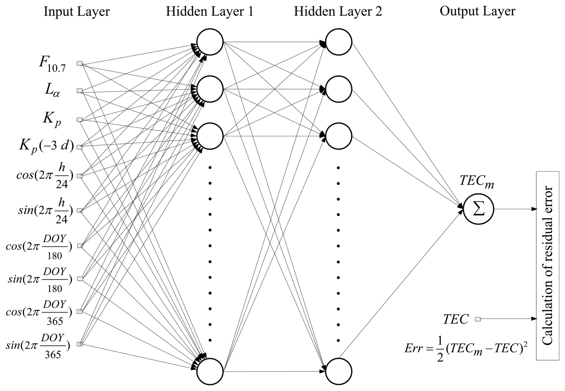
Figure 1 Schematic diagram of the MFFNN for modelling ionospheric TEC in association with solar/geomagnetic activities and seasonal change.

The ML-TEC model fits to the global TEC observation with zero systematic error and a root-mean-square error (RMSE) of 2.8 TECU (TEC unit). This is comparable to the zero systematic error and the RMSE of 3.4 TECU for the empirical function modelling with the global TEC from 1999 to 2011 in Mukhtarov et al. (2013), as well as the RMSE of 3.5 TECU for a statistical model established by Lean et al. (2016) with the global TEC from 1998 to 2015. Figure 2 presents the global maps of the modelled and observed TEC in geographic coordinates. The equatorial ionospheric anomaly (EIA) located between 22.5° S and 25° N and around 105° E, with the summer crest being stronger than the winter one. The Weddell Sea Anomaly is apparent with the stripe amplification between 80 and 50° S and 120° W to 0° E (Mukhtarov et al., 2013). The coincidence of these anomalies indicates that the ML-TEC model is also able to reproduce the spatial structure of the ionosphere.

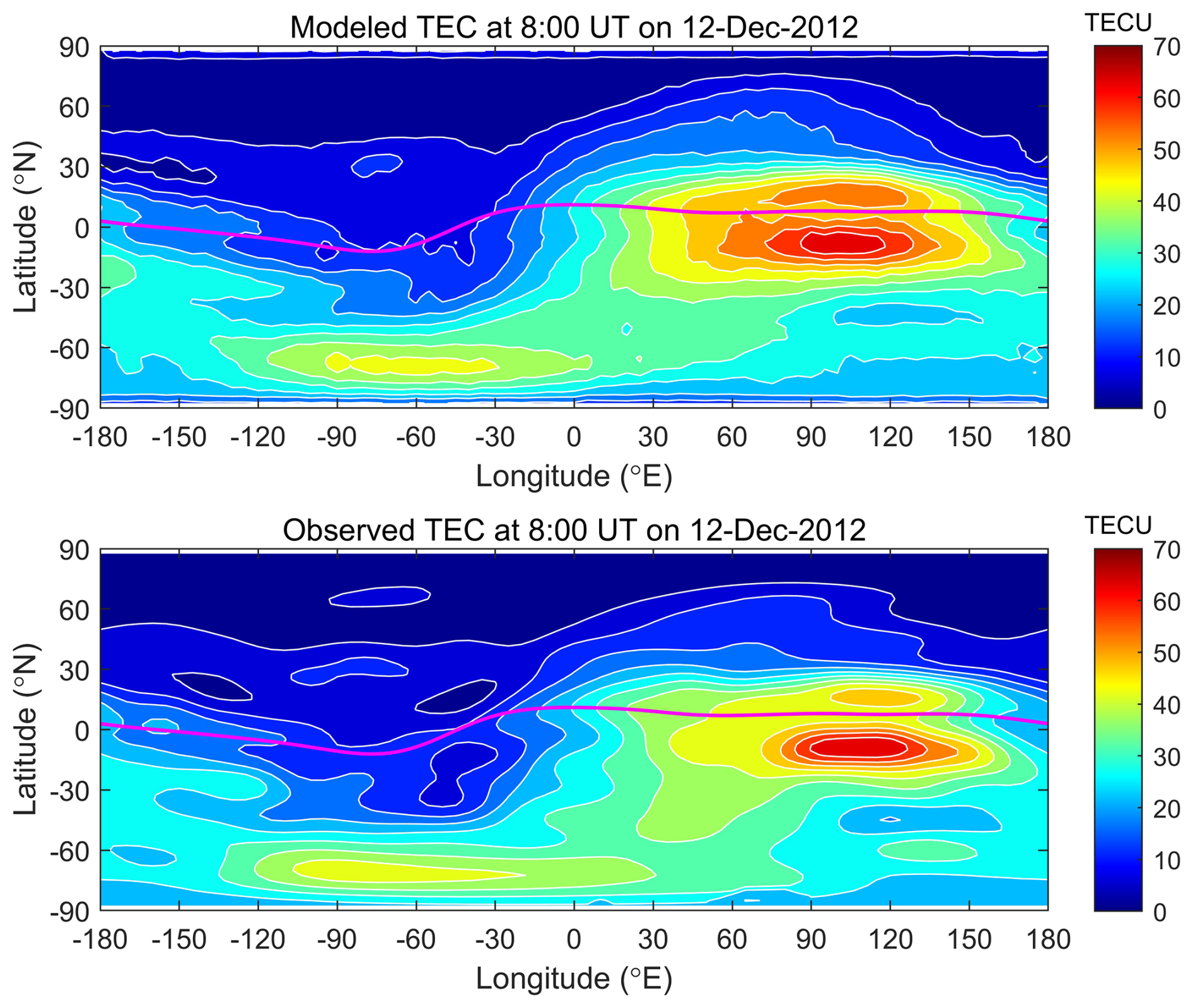
Figure 2 Global maps of the modelled and observed TEC at 08:00 UT on 12 December 2012. The lines in magenta represent the magnetic equator.

The diurnal (s₁) and semidiurnal (s₂) components in TEC time series are obtained with a digital non-recursive, finite-impulse-response (FIR) filter. It performs zero-phase filtering by processing the time series in forward and reverse directions, which helps preserve features in a filtered time waveform exactly where they occur in the unfiltered signal. For bandpass filtering, the cutoff frequencies are at $f_{\mathrm{c}}=f_{\mathrm{p}}\pm \mathrm{10}\mathit{\%}\cdot f_{\mathrm{p}}$, where f_c is the cutoff frequency and f_p is the central frequency. For the diurnal and semidiurnal variations, the cutoff frequencies are $\mathrm{0.9}/\mathrm{1.1}$ and $\mathrm{1.8}/\mathrm{2.2}$ cycles per day (cpd), respectively (Hocke et al., 2024b; Studer et al., 2012).

For the 18 SSW events listed in Table 1, by using the time series of TEC with 2 h resolution, 18 subsets of the observed and modelled global TECs are created that started 200 d before the central date of SSW and ended 200 d after. The flowchart of the further data processing is shown in Fig. 3. For each SSW event, s₁ and s₂ of both the observed and modelled TECs are extracted by applying the FIR filter to the corresponding dataset. They are referred to as s_1o, s_2o, s_1m and s_2m, respectively. With diurnal and semidiurnal components of 18 SSW events, the composite analysis calculates the mean of S₁ and the mean of S₂ for the observed and modelled TECs, represented as S_1o, S_2o, S_1m, and S_2m, respectively. It can be expected that an inherent effect of SSW can be seen in the mean values, while accidental variations that contributed to S₁ and S₂ compensate one another. Then the difference in the composites between observation and model is taken, expressed as ΔS₁ and ΔS₂. This operation removed the solar/geomagnetic and seasonal effects in the diurnal and semidiurnal components, and only those driven by the atmosphere below are retained. As shown by rS₁ and rS₂, the ratios of those observed to the modelled ones are also calculated to show the relative strength of SSW-related disturbances.

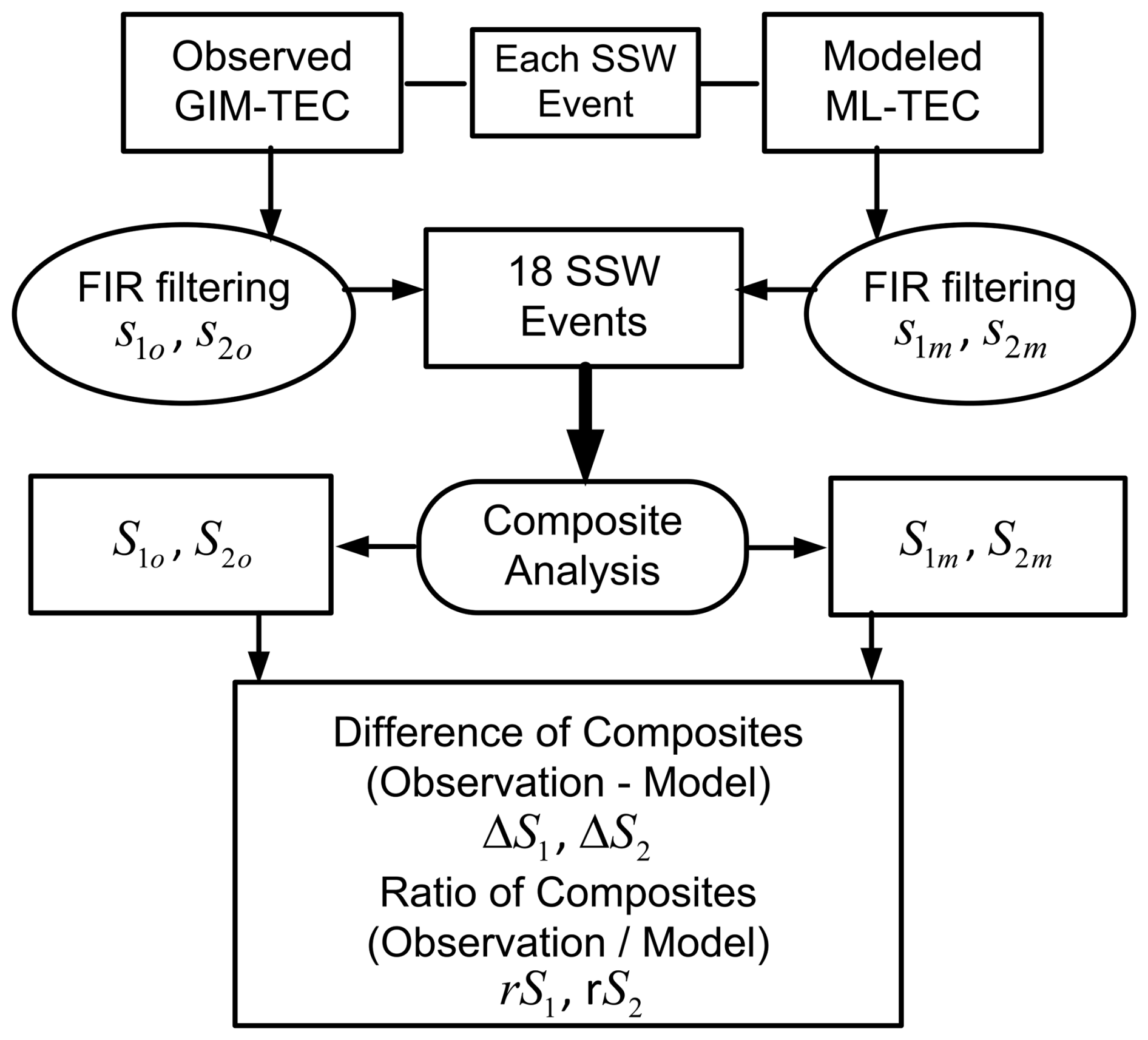
Figure 3 Flowchart of FIR filtering of GIM-TEC and ML-TEC and composite analysis of tidal TEC variations for the 18 SSWs.

3 Results

We begin with a case study for the major SSW event of 25 February 1999 as shown in Fig. 4. The top panel presents the diurnal components at grid point 30° N, 105° E for both the observed GIM-TEC (black line) and modelled ML-TEC (red line). The middle panel is for the semidiurnal components at grid point 30° N, 105° E. The bottom panel gives the F10.7 and K_p indices to show the solar and geomagnetic conditions during the event. The epoch time is from 50 d before the onset of SSW and 100 d after the onset of SSW. The two s₁ time series start to increase around SSW onset, although they are close to each other and oscillate together in the preceding time. The s₁ of the observed TEC is smaller than the model one before SSW onset. However, the s₁ of the observed TEC becomes larger since ∼2 d and shows a maximum at an epoch time of 20 d, which is ∼2.5 TECU larger than the modelled one. The s₁ of the observed TEC remains larger than that of the ML-TEC for ∼30 d. The s₂ of the observed TEC varies in anti-phase with that of the modelled TEC before SSW onset. It starts to become larger than that of the modelled TEC at ∼10 d and reaches a maximum at 20 d. The largest difference is ∼1.6 TECU between the observed and modelled ones. The s₂ of the observed TEC remains larger than that of the modelled TEC for ∼80 d. Note that s₁ from the modelled TEC correlates more with the F10.7 variation, while there is no obvious variation for both s₁ and s₂ corresponding to geomagnetic activities.

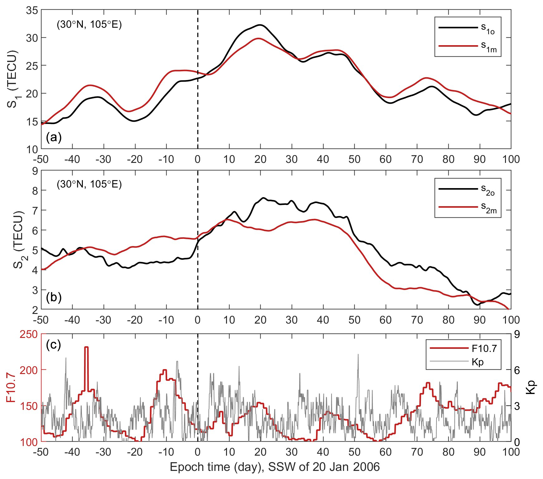
Figure 4 Diurnal variation (a) and semidiurnal variation (b) of TEC at 30° N, 105° E from observed TEC (black lines) during a major SSW event centred on 25 February 1999 (marked as the vertical dashed lines). Shown together are the diurnal and semidiurnal components from modelled TEC (red lines) for the event. The solar and geomagnetic conditions during the event are displayed by F10.7 (red line) and K_p (grey line) (c).

Results of the composite analysis are shown as world maps, latitude–time plots, and longitude–time plots. Since both the diurnal and semidiurnal components vary with latitude, longitude, and time, we select world maps of those with overall smallest values before SSW onset and largest values after SSW onset. For clarity in our description and discussion, we hereafter use the subscript “b” to denote the period before the SSW onset and the subscript “a” to denote the period after the SSW onset. Fig. 5 exhibits world maps of diurnal variation from composite analysis of the 18 SSW events at 13 d before SSW onset and 25 d after SSW onset. The thick black line in each map depicts the magnetic equator. In the left panel (ΔS_1b) is the global ΔS₁ at 13 d before SSW onset. Conspicuous negative ΔS_1b occupies most of the land areas. Positive ΔS_1b is located mainly over oceans and from high latitudes to polar regions. However, it can also be spotted over lands in the midlatitudes of the Northern Hemisphere and the low latitudes in the Southern Hemisphere. Shown in Fig. 5b, at 25 d after SSW onset, is conspicuous positive ΔS_1a, which prevails almost globally. The largest values are located around the EIA in the Northern Hemisphere. It appears with moderate strength around 90° E, 75° W in the middle to high latitudes in the Northern Hemisphere and in the middle to high latitudes for all longitudes in the Southern Hemisphere. There are also positive patches in low latitudes in South America and to its west. By contrasting ΔS_1a and ΔS_1b, the amount of change, referred to as ΔS_1E, can be obtained by taking the difference, i.e. ΔS_1a−ΔS_1b. An enhancement (positive ΔS_1E) can be discerned globally. The enhancement larger than 1.0 TECU is mainly distributed at low northern latitudes in a longitudinal range of 135° W to 100° E. The largest ΔS_1E is 1.5 TECU and is located at 5° N, 85° W. In the Southern Hemisphere, ΔS_1E can be larger than 1.0 TECU from low to high latitudes around 75° W in the American sector. Therefore, the enhancement is generally stronger in the Northern Hemisphere than the Southern Hemisphere. Figure 5c is for rS₁ at 13 d before SSW onset, and Fig. 5d is at 25 d after SSW onset. The rS₁ value larger than 1 matches positive ΔS₁, and the rS₁ value smaller than 1 matches negative ΔS₁. Similar spatial distributions can be noticed similarly to those of ΔS₁ by comparing the corresponding maps in the left panels. At 25 d after SSW onset, rS_1a is also stronger in the Northern Hemisphere than the Southern Hemisphere. However, it has a similar level at the Northern Hemisphere low and middle latitudes. Note that the largest rS₁ is located at high latitudes near polar regions, which is different from that of ΔS₁. This can be attributed to the small values of diurnal variation due to the smaller TEC there compared to low to middle latitudes.

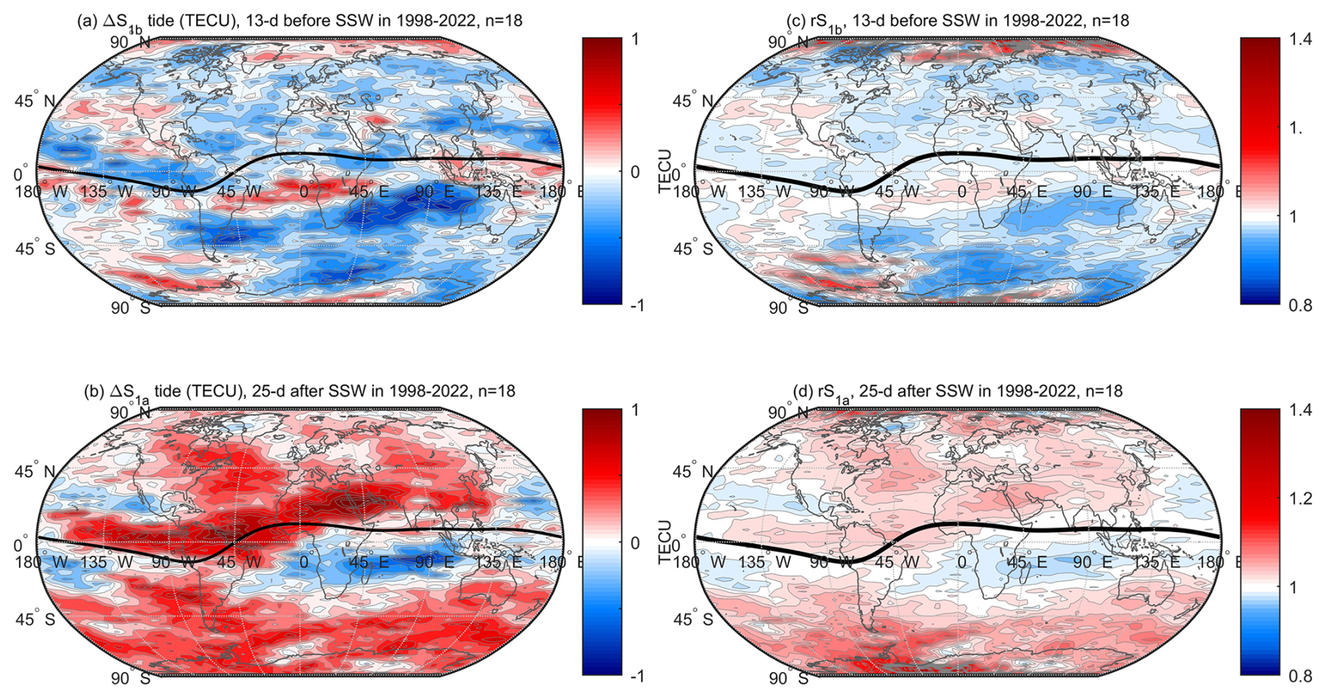
Figure 5 Distributions of ΔS₁ and rS₁ from composite analysis of the 18 SSW events at 13 d before SSW onset and 25 d after SSW onset with (a) for ΔS_1b, (b) for ΔS_1a, (c) for rS_1b, and (d) for rS_1a. The thick black line in each map depicts the magnetic equator.

The global distributions of semidiurnal TEC variation are shown in Fig. 6 with panel (a) showing the global ΔS_2b at 12 d before SSW onset and panel (b) showing ΔS_2a at 8 d after SSW onset in the left panels, and those corresponding to rS₂ are in the right panels. At 12 d before SSW onset, ΔS_2b is generally between −0.5 and 0.8 TECU in magnitude. In the Northern Hemisphere, positive ΔS_2b values manifest as patches at low latitudes along the magnetic equator, although a few larger patches can be seen at middle and high latitudes. In the Southern Hemisphere, ΔS_2b is more active with red patches or belts that fill at low to middle latitudes and high latitudes in the American, Atlantic, and Asian sectors. At 8 d after SSW onset, ΔS_2a peaks along the magnetic equator at EIA in both hemispheres with the largest value of 2.0 TECU around 30° S, 85° W. The red belt is generally wider in the Southern Hemisphere than the Northern Hemisphere. By contrasting ΔS_2a and ΔS_2b, $\mathrm{\Delta }{S}_{\mathrm{2}\mathrm{E}}=\mathrm{\Delta }{S}_{\mathrm{2}\mathrm{a}}-\mathrm{\Delta }{S}_{\mathrm{2}\mathrm{b}}$, we can perceive an enhancement in the Northern Hemisphere in most areas except Russia, eastern Europe, central North America, and the Pacific Ocean at ∼45° N. In the Southern Hemisphere, strong enhancement is more widespread, and only several small white patches can be seen with much smaller areas. In land areas, the largest ΔS_2E is 1.5 TECU at 32.5° S, 80° W, though it can reach 1.8 TECU around $\pm \sim \mathrm{20}$° N over the Pacific Ocean. The right panel of Fig. 6 shows rS₂ with panel (c) at 12 d before SSW onset and panel (d) at 8 d after SSW onset. There are also similar relationships between rS₂ and ΔS₂ by comparing the corresponding maps in the two panels. At 12 d after SSW onset, rS_2a is obviously stronger in the Southern Hemisphere than the Northern Hemisphere.

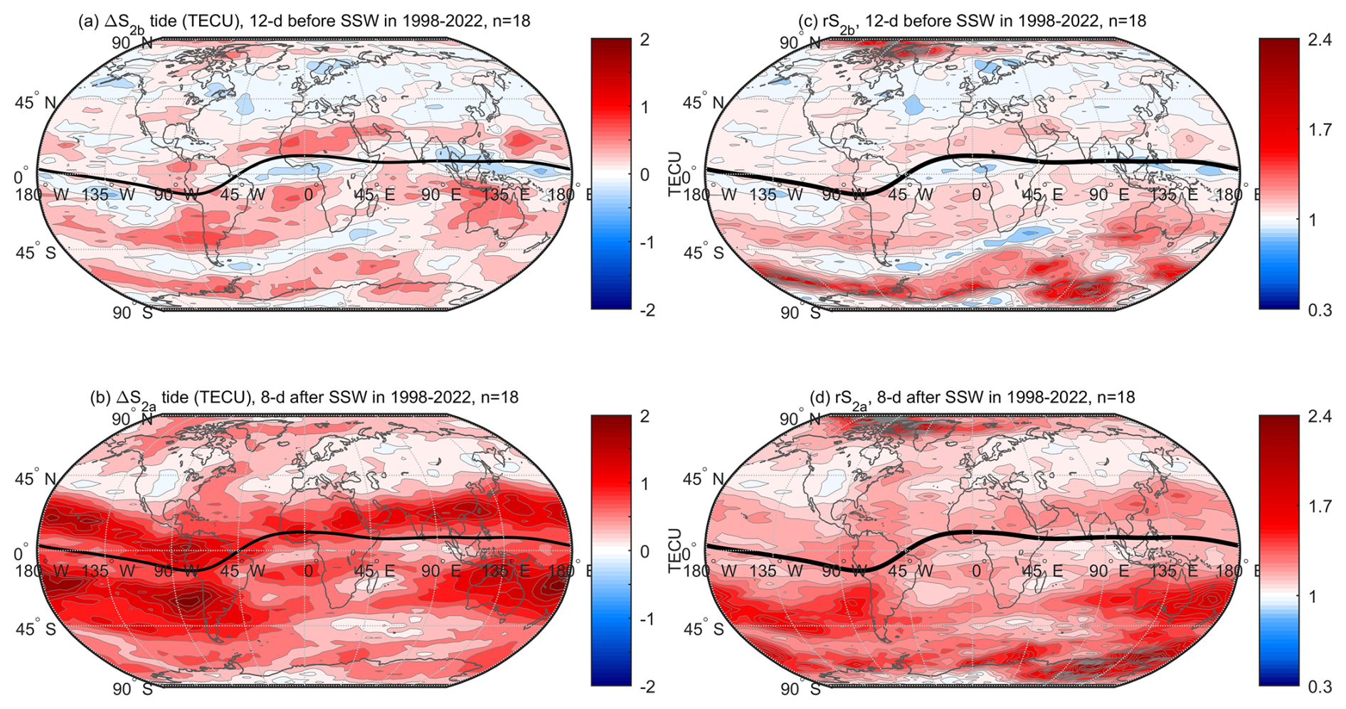
Figure 6 Distributions of ΔS₂ and rS₂ from composite analysis of the 18 SSW events at 12 d before SSW onset and 8 d after SSW onset (b) with (a) for ΔS_2b, (b) for ΔS_2a, (c) for rS_2b, and (d) for rS_2a. The thick black line in each map depicts the magnetic equator.

It is important to examine the ionospheric tidal variabilities at different longitudes over time. We select two longitudes of 90° E and 75° W to examine the temporal variations of ΔS₁ and ΔS₂. As shown above by Figs. 5 and 6, at ∼90° E there is an obvious enhancement of the diurnal component in northern midlatitudes; at 75° W, a prominent enhancement of both diurnal and semidiurnal components can be seen in both hemispheres. Figure 7 shows the time variation of ΔS₁ and ΔS₂ at 90° E, which is smoothed as a 14 d average. An enhancement of ΔS₁ can be seen from the SSW onset to ∼35 d after the SSW onset in the whole northern latitudes. At ∼25° N, the prominent positive ΔS₁ starts to appear simultaneously as the onset day of SSW and ends at ∼40 d. The strongest enhancement happens from ∼15 to ∼35° N. At ∼25° N, ΔS₁ shows a peak level of ∼0.6 TECU around 10 d, and it maintains the highest level from 0 to ∼35 d after the SSW onset. Concerning the semidiurnal component, clear enhancement of ΔS₂ starts just from the SSW onset in the Northern Hemisphere. The enhancement ends at ∼35 d in midlatitudes and ∼50 d at low to middle latitudes. The largest ΔS₂ is 1.3 TECU, centring around ∼20° N and ∼8 d after SSW onset. Note that there is no systematic enhancement during the entire SSW at 90° E in the Southern Hemisphere with only a few GNSS receivers due to the ocean.

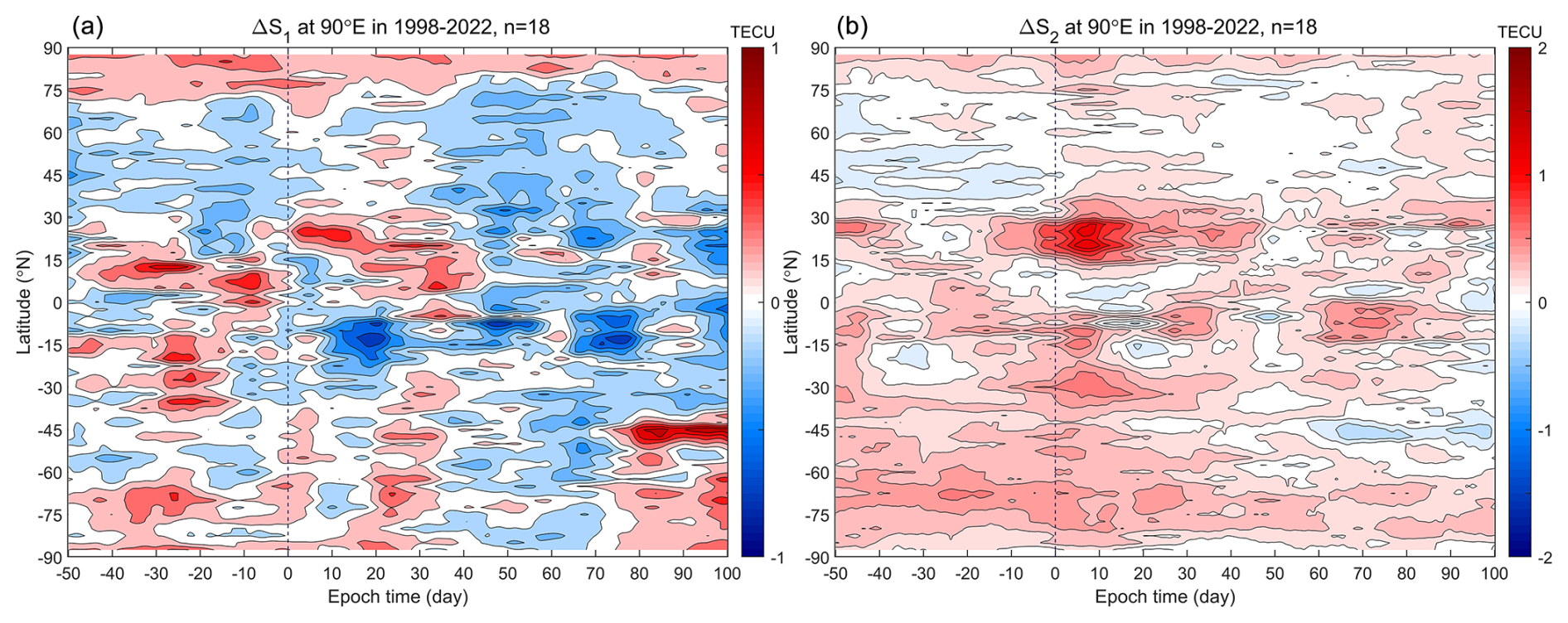
Figure 7 Time variation of meridian ΔS₁ (a) and ΔS₂ (b) at 90° E, which is smoothed as a 14 d moving average. The vertical dashed lines mark the SSW onset day.

Figure 8 shows the meridian plot of smoothed ΔS₁ and ΔS₂ at 75° W (denoted −75° E in figures). It is obvious that from ∼0 to ∼70° N an enhancement of ΔS₁ starts from the SSW onset; it ends at ∼50 d in low latitudes and at ∼30 d in middle to high latitudes. At ∼2.5° N, ΔS₁ increases very quickly and maintains a high level from ∼8 to 22 d with the largest value of 0.8 TECU. In the Southern Hemisphere, the enhancement of ΔS₁ is delayed with latitude to ∼30° S. For ΔS₂, an enhancement takes place in the whole meridian from the SSW onset to ∼55 d after the SSW onset, except latitudes larger than 50° S in the Southern Hemisphere. The prominent enhancement occurs in the range from 50° S to 40° N, respectively. The striking positive ΔS₂ starts to appear at about −10 d before the SSW onset, reaches a maximum at ∼8 d and ends at ∼50 d after the SSW onset at both EIA regions. Note that ΔS₂ has another peak at ∼25 d at the northern EIA. Between ∼30° S and ∼2.5° N, ΔS₂ starts to increase at ∼10 d before SSW onset, reaches to its first peak of ∼1.5 TECU in the period of 3–9 d and the second peak at ∼25 d after SSW onset.

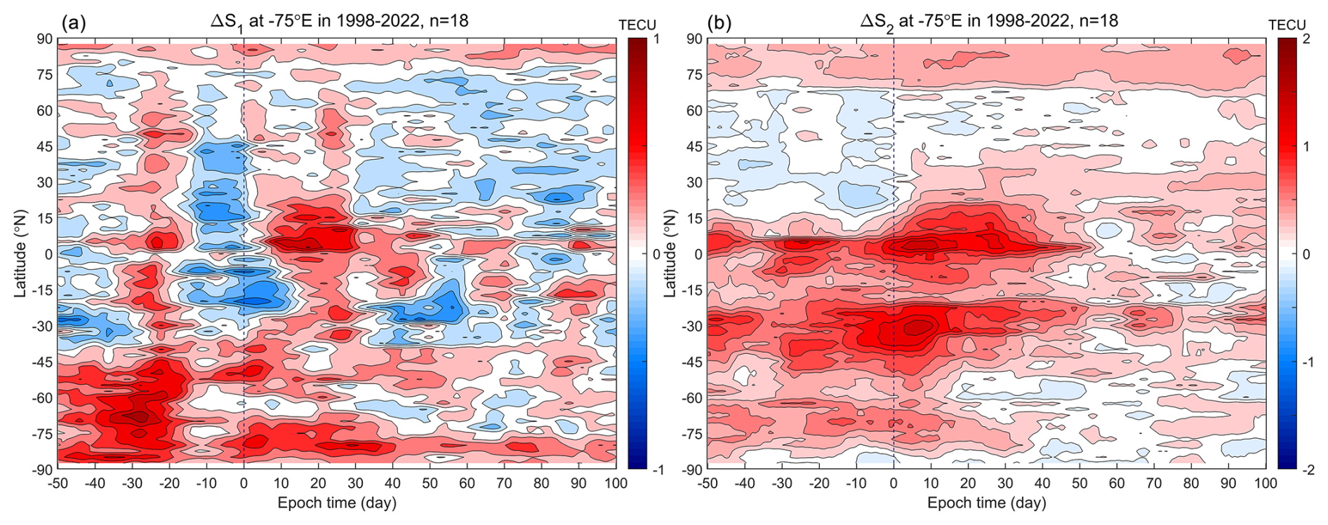
Figure 8 Time variation of meridian ΔS₁ (a) and ΔS₂ (b) at “−75° E”, which is smoothed as a 14 d moving average. The vertical dashed lines mark the SSW onset day.

It is also worthwhile to study the global temporal variation at specific latitude. Figure 9 plots the temporal variation of ΔS₁ and ΔS₂ at the latitude of 22.5° N, which is smoothed as a 14 d moving average. The ΔS₁ generally starts to increase at the SSW onset and keeps positive for ∼30 d. It shows a maximum of 1.0 TECU around 20–26 d after the SSW onset. The zonal ΔS₂ at 22.5° N basically shows temporal variation synchronously although the values of ΔS₂ are different at different longitudes. It reaches a maximum of ∼1.4 TECU at ∼120° E and ∼8 d after the SSW onset. ΔS₂ between 60–135° E returns to the SSW onset level at ∼45 d. ΔS₂ between 120° W and 60° E decreases to the SSW onset level at ∼30 d. Over the western Pacific Ocean, it returns to the onset level at ∼20 d. We notice that positive ΔS₁ and ΔS₂ also occur and last for days before SSW onset. However, they are generally smaller, shorter-lived, and slower-varying than those after SSW onset.

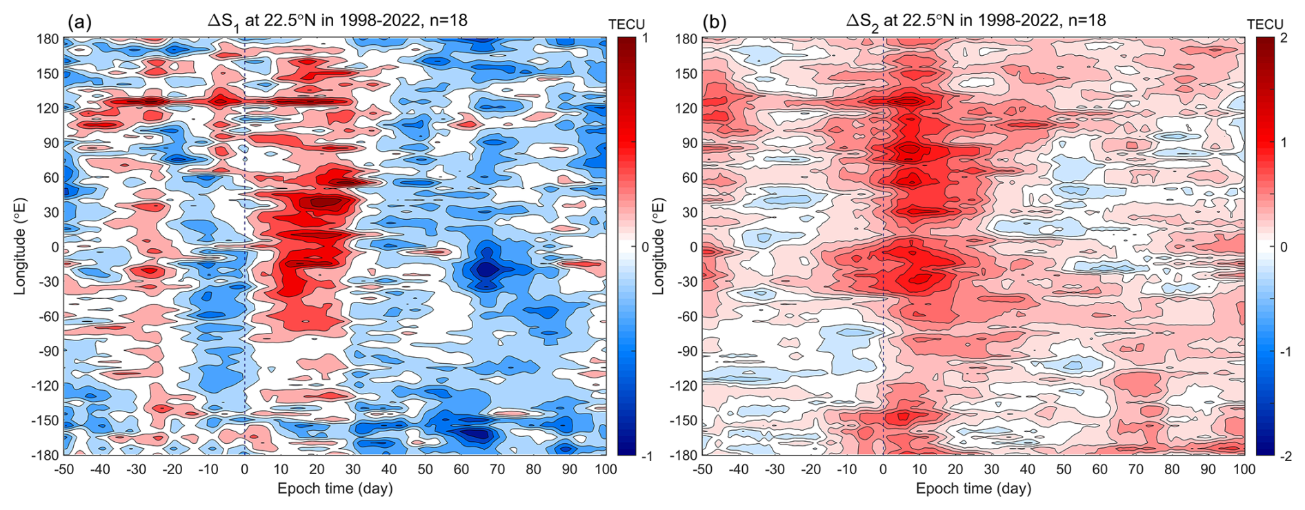
Figure 9 Time variation of zonal ΔS₁ (a) and ΔS₂ (b) at 22.5° N, which is smoothed as a 14 d moving average. The vertical dashed lines mark the SSW onset day.

4 Discussion

The driving factors of the ionosphere consist of solar and magnetospheric energies from above and the atmospheric forcing from below. For the attribution of ionospheric response to SSW, it is crucial to separate the atmospheric waves from effects due to solar/magnetospheric variability and seasonal variation. The case study of the SSW on 25 February 1999 in Fig. 4 shows intensified diurnal/semidiurnal variations of the observed TEC at 30° N after the SSW onset. The diurnal/semidiurnal components from modelled TEC manifest as a contribution from solar/magnetospheric energies and seasonal change. The comparison between the observation and model suggests a clear SSW effect on the low-latitude ionosphere, which is in agreement with previous studies (Chau et al., 2012; Liu et al., 2019).

Since the ionosphere has local characteristics and since each SSW event may have a different effect due to complicated solar–terrestrial conditions, it is justifiable to perform the composite analysis described in the above analysis method. The 18 SSW events happened from 1998 to 2022, which cover two solar activity cycles. The composite analysis with the solar and magnetospheric effects removed would provide unambiguous evaluation of the SSW effects on the global ionosphere.

The world maps and temporal variations over latitude/longitude of diurnal and semidiurnal components from our composite analysis in Figs. 5–9 reveal that the SSW effects are indeed global as depicted by Pedatella et al. (2018). SSW-induced amplifications of diurnal/semidiurnal tides can be identified from low to high latitudes with the strongest at EIA crests along the magnetic equator. Amplifications in semidiurnal tides during SSWs have been revealed in the low-latitude ionosphere from both case studies and statistical studies (Chau et al., 2012; Goncharenko et al., 2021; Hocke et al., 2024b). Semidiurnal disturbances in the midlatitude ionosphere have only been observed in Asian and American sectors in the Northern Hemisphere (Xiong et al., 2013; Chen et al., 2016; Goncharenko et al., 2013; Liu et al., 2019). Our observation not only confirms the previous results, but also displays that the semidiurnal pattern in the midlatitude ionosphere during SSWs is a global phenomenon. Interestingly, the semidiurnal enhancement is stronger in the Southern Hemisphere midlatitudes than in the Northern Hemisphere. Several SSW event studies have highlighted that semidiurnal tides in the Southern Hemisphere midlatitudes, particularly around 75° W in the American sector, are stronger than those in the Northern Hemisphere. This hemispheric asymmetry may arise from the amplification of lunar semidiurnal (M2) tides during SSWs, which is the most pronounced in the American sector (Goncharenko et al., 2021; Liu et al., 2021, 2022). Additionally, the inclination angle of Earth's magnetic field lines in the Southern Hemisphere midlatitudes is smaller than in the Northern Hemisphere, leading to more ionospheric TEC variations in the F-region due to electric field effects (Goncharenko et al., 2022).

Concerning the diurnal variability, enhancement was observed at low latitudes and at the midlatitude site of Mohe (53.5° N, 122.3° E) for the SSW event in 2018 (Liu et al., 2019). Our study reveals, for the first time, that diurnal TEC variations exhibit a global enhancement pattern, with stronger effects in the Northern Hemisphere than the Southern Hemisphere. This contrasts with the semidiurnal enhancement, which is stronger in the Southern Hemisphere. Longitudinal differences are also evident, with weaker amplification in the Atlantic, African, and Indian sectors, particularly for the diurnal tide in the Southern Hemisphere. Recently, Harvey et al. (2022) emphasized the influence of the mesospheric polar vortex on atmospheric tides, which helps explain this hemispheric asymmetry. Since major SSWs occur predominantly in the Northern Hemisphere during winter, the mesospheric polar vortex in the Northern Hemisphere significantly modulates the upward propagation of atmospheric tides to the ionosphere. This process enhances the diurnal variation of TEC, making it more pronounced in the Northern Hemisphere.

Temporally, the global diurnal component (ΔS₁) at 22.5° N starts to increase simultaneously on the day of SSW onset, peaking around 20–26 d later and lasting for approximately 30 d (Figs. 9). In contrast, the semidiurnal component (ΔS₂) at 75° W starts to increase simultaneously at ∼10 d before SSW onset. It peaks at ∼8 d and persists for ∼50 d after the SSW onset (Fig. 8). At other longitudes shown in Fig. 9, the semidiurnal component starts to enhance at ∼20 d before SSW onset and peaks at ∼8 d after SSW onset. Note that the enhancement generally lasts ∼50 d during SSW with the prominent effect happening between 45° W and 120° E. These findings align with the review by Goncharenko et al. (2021), which has summarized that the main SSW effect is a distinct semidiurnal variation in thermospheric and ionospheric parameters that lasts for days up to 30–40 d. The results of our comprehensive composite analysis for 18 SSW events demonstrate that the enhancement of the diurnal and semidiurnal components last for ∼30 and ∼50 d, respectively. While the semidiurnal enhancement starts earlier and peaks at ∼8 d after SSW onset, the diurnal one starts on the SSW onset day and peaks around 20–26 d later.

The SSW effects on the tidal ionospheric TEC variations are a global phenomenon. The complicated patterns of the SSW-induced tidal ionospheric TEC variations indicate that multiple dynamic processes might be involved during SSWs. We speculate that the SSW-related E-region dynamo is the main mechanism which is generally larger in the low-latitude ionosphere to produce more significant vertical plasma drifts than midlatitudes.

5 Conclusions

We present a comprehensive composite analysis of the ionospheric tidal variability associated with 18 sudden stratospheric warming events by using the global total electron content data from 1998 to 2022. To extract TEC variations from effects of SSWs and atmospheric forcing below the ionosphere, we first model the TEC climatology due to solar activity, magnetospheric energy, and seasonal change by neural network training for the observed time series of global TEC; then we remove the modelled TEC from the observed TEC. Our analysis reveals for the first time a globally SSW-induced enhancement in both semidiurnal and diurnal TEC variations. Key findings include the following:

1. Semidiurnal TEC variations. The strongest enhancements occur at the EIA crests along the magnetic equator, consistent with previous studies. At midlatitudes, the semidiurnal enhancement is stronger in the Southern Hemisphere than in the Northern Hemisphere, likely due to the amplification of lunar semidiurnal tides (M2) and differences in geomagnetic field geometry.

2. Diurnal TEC variations. Diurnal enhancements exhibit a global pattern, with stronger effects in the Northern Hemisphere midlatitudes compared to the Southern Hemisphere, contrasting with the semidiurnal enhancement.

3. Temporal evolution. The semidiurnal enhancement starts ∼10 d before the SSW onset, peaks at ∼8 d after the onset, and lasts for ∼50 d. In contrast, the diurnal enhancement begins on the SSW onset day, peaks around 20–26 d later, and persists for ∼30 d.

4. Longitudinal dependence. Both diurnal and semidiurnal enhancements show longitudinal variability, with weaker amplification in the Atlantic, African, and Indian sectors, particularly for the diurnal tide in the Southern Hemisphere.

Our analysis indicates that multiple dynamic processes might be involved during SSWs from the hemispheric asymmetry and longitudinal differences in diurnal/semidiurnal variations of TEC. It is likely that the SSW-related E-region dynamo is the main mechanism which is generally strong enough to produce discernible TEC variations in the low- to midlatitude ionosphere. The ML-TEC model can separate the SSW effects on the ionosphere from dependences on solar/geomagnetic activities and season. This is a new analysis method which is important for SSW analysis since the tidal amplitudes in the upper atmosphere have a strong seasonal dependence. The regular, seasonal enhancement of tidal amplitudes in Northern Hemisphere winter can be wrongly attributed to SSWs since SSWs mainly happen in Northern Hemisphere winter. Our ML-TEC model avoids such a false attribution.