Locating and quantifying CH₄ sources within a wastewater treatment plant based on mobile measurements

Wastewater treatment plants (WWTPs) are substantial contributors of greenhouse gas (GHG) emissions because of the high production of methane (CH₄) and nitrous oxide (N₂O). A typical WWTP complex contains multiple functional areas that are potential sources of GHG emissions. Accurately quantifying GHG emissions from these sources is challenging due to the inaccuracy of activity data, the ambiguity of emission sources, and the absence of monitoring standards. Locating and quantifying WWTP emission sources using a measurement-based GHG emission quantification method is crucial for evaluating and improving traditional emission inventories. In this study, CH₄ mobile measurements were conducted within a WWTP complex in the summer and winter of 2023. We utilized a multi-source Gaussian plume model combined with a genetic algorithm inversion framework, designed to locate major sources within the plant and quantify the corresponding CH₄ emission fluxes. We identified 13 main sources in the plant and estimated plant-scale CH₄ emission fluxes of $\mathrm{68.78}\pm \mathrm{17.40}\mathrm{kg}{\mathrm{h}}^{-\mathrm{1}}$ ($\mathrm{603.33}\pm \mathrm{152.66}\mathrm{t}{\mathrm{a}}^{-\mathrm{1}}$) for the summer and $\mathrm{47.76}\pm \mathrm{21.39}\mathrm{kg}{\mathrm{h}}^{-\mathrm{1}}$ ($\mathrm{418.95}\pm \mathrm{187.59}\mathrm{t}{\mathrm{a}}^{-\mathrm{1}}$) for the winter. The predominant sources of CH₄ emissions were the screen and primary clarifier, contributing 55 % and 67 % to the total emissions in summer and winter, respectively. The comparison revealed that summer CH₄ emissions were 2.8 times higher than inventory estimates, while winter emissions were twice the inventory values. This study demonstrated that mobile measurements, combined with the multi-source Gaussian plume inversion framework, are a powerful tool to locate and quantify GHG sources at a complex site, with the potential for further refinement to accommodate different types of factories and gas species.

1 Introduction

Methane (CH₄) is the second-largest contributor to climate change, with a global warming potential 27.9 times that of carbon dioxide (CO₂). Thus, reducing CH₄ emissions is essential for mitigating climate change and progressively achieving the global target of limiting warming to 1.5 °C (IPCC, 2023). The World Meteorological Organization Global Atmospheric Watch network indicated that the global annual average concentration of CH₄ in 2022 was 1923±2 ppb, representing a 264 % increase from preindustrial levels (WMO, 2023). The International Energy Agency (IEA) “Global Methane Tracker 2024” report suggested that global CH₄ emissions reached 580 Mt in 2023, with anthropogenic CH₄ emissions accounting for 60 % of this amount. The complexity of CH₄ emission processes, the lack of monitoring systems, and the limitations of emission estimation models present challenges with respect to accurately estimating anthropogenic CH₄ emissions.

The quantification of CH₄ emission fluxes is typically achieved through a bottom-up inventory method. However, due to the difficulties in obtaining activity data used for actual emission factors and the paucity of specific information on different emission sources, there is considerable uncertainty in assessments using the emission inventory method (Lin et al., 2021). In contrast, a top-down method that estimates CH₄ emissions by monitoring the atmospheric concentration has been increasingly applied in recent years (Sun et al., 2019; Cusworth et al., 2024; Han et al., 2024; Maazallahi et al., 2023; Riddick et al., 2017). The monitoring technology mainly includes satellite (Zhang et al., 2021; Liang et al., 2023; Jacob et al., 2022) and airborne (Allen et al., 2019; Abeywickrama et al., 2023; Cui et al., 2017) remote sensing as well as ground-based monitoring, such as vehicle-based mobile monitoring (Albertson et al., 2016; Al-Shalan et al., 2022; Caulton et al., 2018), station monitoring (Dietrich et al., 2021; Hase et al., 2015; Heerah et al.,2021), and tower monitoring (Richardson et al., 2017; Balashov et al., 2020). Emission flux inversion methods also include the isotope tracer method (Jackson et al., 2014; Zimnoch et al., 2018), the cross-sectional flux method (Luther et al., 2019; Makarova et al., 2021), and the atmospheric diffusion model inversion method (Kumar et al., 2021; Yacovitch et al., 2015). Atmospheric transport models with varied degrees of complexity, including Gaussian diffusion models (Stadler et al., 2021), Lagrangian models (McKain et al., 2015), and Eulerian models (Bergamaschi et al., 2018), are used in the inversion to relate greenhouse gas (GHG) concentrations to emissions. Optimization methods, such as Bayesian optimization (Karion et al., 2019) and linear regression models (Kumar et al., 2021), are applied to achieve accurate inversion results. Furthermore, some studies have incorporated carbon isotope observations to better attribute the contribution of different CH₄ emission sources (Maazallahi et al., 2020). Numerous studies have used satellite remote sensing, uncrewed aerial vehicle (UAV) monitoring, and vehicle-based mobile monitoring techniques to measure CH₄ emissions (Sun et al., 2023). However, satellite spatiotemporal resolution is limited and UAVs have short endurance, making vehicle-based mobile monitoring a better choice for measuring CH₄ emissions. Vehicle-based mobile monitoring can perform the continuous real-time monitoring and precise identification of emission sources and, hence, has been applied for the urban (von Fischer et al., 2017; Defratyka et al., 2021) and plant-scale (Zhao et al., 2021; Jin et al., 2010) monitoring of GHG concentrations and emission fluxes. Vogel et al. (2024) used high-precision, fast-response GHG analyzers to investigate CH₄ leaks in 12 cities across eight countries. Chen et al. (2020) utilized the multiple-Gaussian-plume model for mobile measurements of CH₄ emissions during the Munich Oktoberfest. Shi et al. (2023) conducted mobile measurements with a vehicle-based monitoring system at chemical, coal washing, and waste incineration plants in two cities and one industrial park in China.

As a significant source of GHG emissions, wastewater treatment plants (WWTPs) generate substantial amounts of CH₄, N₂O, and CO₂ during the collection, treatment, and discharge of sewage and sludge, contributing 3 % of the global total GHG emissions (Bai et al., 2022). The estimation of CH₄ emission fluxes from WWTPs has increasingly attracted widespread attention. Li et al. (2024) developed a plant-level and technology-based CH₄ emission inventory for municipal WWTPs in China, estimating the CH₄ emissions for 2020 to be 150.6 Gg. Delre et al. (2017) measured the CH₄ concentrations downwind of five WWTPs in Scandinavia using tracer gas dispersion, obtaining a range of CH₄ emission fluxes from 1.1±0.1 to $\mathrm{18.1}\pm \mathrm{6.3}\mathrm{kg}{\mathrm{h}}^{-\mathrm{1}}$. Moore et al. (2023) employed CH₄ mobile measurements from 63 WWTPs in the USA, pointing to a significant underestimation in the CH₄ emission inventories. However, most studies lack comparisons between measured and simulated concentrations, resulting in significant uncertainty in the results. We present a mobile measurement investigation of a WWTP in Hangzhou in 2023. To analyze the mobile data, we constructed a multi-source Gaussian plume model combined with a genetic algorithm inversion framework, which assisted us in locating and quantifying CH₄ emission sources, based on the concentration distribution measured within the WWTP. Additionally, we compared CH₄ emission fluxes from the measurements with the bottom-up estimates of emission inventories. A sensitivity analysis was performed to elucidate the discrepancies arising from variations in emission source locations. Our results provide insight into the formulation and evaluation of emission reduction measures for WWTPs.

2 Instruments and methods

2.1 Site selection

With respect to the monitoring site, a WWTP in Hangzhou, a megacity in East China, was chosen. This WWTP is a large-scale plant, processing up to 1.5×10⁶ t of domestic wastewater daily. The chosen WWTP processes encompass mechanical treatment, biological treatment, sedimentation, advanced treatment, disinfection, and sludge treatment. As illustrated in Fig. 1, we divide the WWTP into 14 functional areas according to treatment processes. Areas associated with primary treatment were labeled as coarse screens and primary sedimentation tanks, whereas those linked to secondary treatment were indicated as aeration tanks and secondary sedimentation tanks. We performed one monitoring experiment per day, with each experiment entailing one to two rounds of mobile measurements along external roads and along internal roads around the functional areas. Additionally, we conducted repeated mobile measurements and fixed measurements on roads with high concentrations to calculate average concentration data. Over 10 d of experiments from June to December 2023, we obtain 8 d of complete monitoring data, including 3 d in summer and 5 d in winter. On the other 2 experimental days, internal facility maintenance restricted access to certain roads, resulting in incomplete monitoring data.

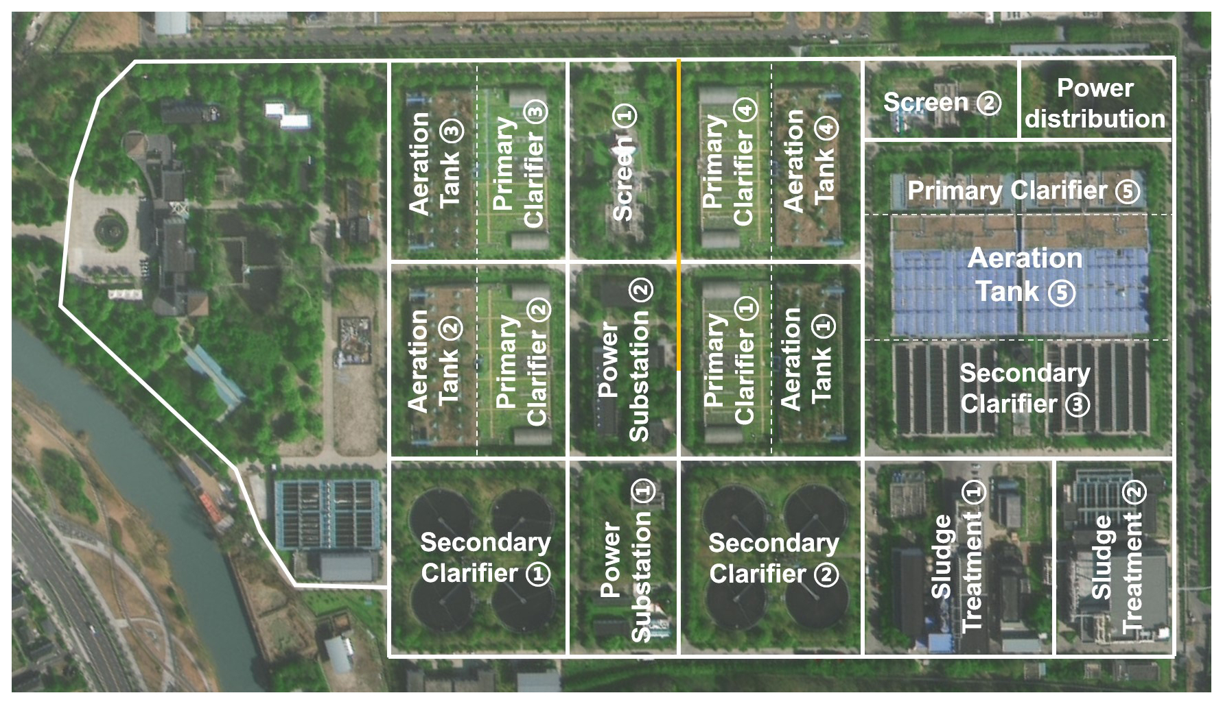
Figure 1 Distribution of the WWTP functional areas. The yellow mark represents the simulated location of the line source. Solid lines show the roads measured by the mobile vehicle. Map data are from Esri.

2.2 Instrumentation

The monitoring instruments consisted of a vehicle-mounted cavity ring-down spectrometer (CRDS) monitoring system (Zhao et al., 2024) and a portable meteorological station. The vehicle-mounted CRDS system was anchored by the CRDS analyzer (Picarro G2201-i, Picarro 2010), accompanied by GPS and meteorological instruments. The volume fraction of CH₄ is measured with an accuracy of 5 ppb±0.05 %. CRDS measurements have the advantages of strong interference resistance and high sensitivity and accuracy, making them widely employed in research focused on monitoring GHG emissions (Rella et al., 2015; Lopez et al., 2017).

In this study, the CRDS analyzer was placed inside the monitoring vehicle to measure CH₄ concentrations in the WWTP. The sampling probe was placed near the roof along the window of the car to avoid interference from vehicle exhaust due to the low position. The mobile meteorological instrument was placed on the roof of the vehicle to gather meteorological data. In addition, the GPS unit was integrated to record the location of sampling points during the measurement period. Two portable meteorological stations (SWS-500, Hangzhou Pengpu Technology), capable of measuring meteorological parameters (wind speed, direction, temperature, humidity, and atmospheric pressure), were positioned adjacent to the main entrance and atop the filter tank at the WWTP.

2.3 Inventory accounting method

We used the methods suggested by the Intergovernmental Panel on Climate Change (IPCC, 2006) to calculate the CH₄ emissions from wastewater. The formula for calculating the CH₄ emissions from wastewater is described as follows:

$$\begin{array}{}\text{(1)}& E_{{\mathrm{CH}}_{\mathrm{4}}}=(\text{TOW}-S\cdot a)\cdot {\text{EF}}_{{\mathrm{CH}}_{\mathrm{4}}}-R_{{\mathrm{CH}}_{\mathrm{4}}},\end{array}$$

where $E_{{\mathrm{CH}}_{\mathrm{4}}}$ denotes the direct CH₄ emissions from the wastewater treatment plant (t CH₄ a⁻¹), total organic waste (TOW) is defined as the total organic pollutant load in the influent wastewater (t COD a⁻¹ – chemical oxygen demand per year), S refers to the annual production total of dry sludge (t a⁻¹), the parameter a signifies the organic matter content in the dry sludge (t COD t⁻¹), ${\text{EF}}_{{\mathrm{CH}}_{\mathrm{4}}}$ is the CH₄ emission factor (t CH₄ t COD⁻¹), and $R_{{\mathrm{CH}}_{\mathrm{4}}}$ quantifies the annual recovery of CH₄ from anaerobic treatment processes (t a⁻¹).

Operational data for the WWTP examined in this study were derived from the “Urban Drainage Statistical Yearbook”, an annual publication of the urban water supply and drainage systems in China. This dataset includes details such as the water treatment volume, sludge production, and the concentrations of six pollutants (COD_Cr, biochemical oxygen demand (BOD), suspended solid (SS), NH₃–N, total nitrogen (TN), and total phosphorus (TP)) in both influent and effluent. TOW is calculated using the amount of treated water and the COD influent concentration of the WWTP provided in the yearbook, while the annual sludge production (S) is extracted directly from the yearbook. The organic matter content in dry sludge is estimated at an empirical 40 %, assuming a sludge moisture content of 75 %, leading to a value of 0.1 (Guo et al., 2019). ${\text{EF}}_{{\mathrm{CH}}_{\mathrm{4}}}$ is selected based on the recommended value of 0.0046 for Zhejiang Province (Cai et al., 2015). Given the infrequency of anaerobic treatment in wastewater, $R_{{\mathrm{CH}}_{\mathrm{4}}}$ is set to zero.

2.4 Inversion method

We developed an inversion framework for emission fluxes designed for plant-level applications. The framework used mobile measurement data, the locations of emission sources, and initial emission estimates, alongside wind speed and direction data, as inputs to the multi-source Gaussian diffusion models. The preliminary localization of the emission sources was chiefly contingent upon the concentration distribution along the roads within the internal functional areas. Meanwhile, the initial emission estimates for each source were determined by integrating the concentration data from these areas with an improved empirical equation (Weller et al., 2019). Based on the comparison of measurements and model simulation results (Fig. S1 in the Supplement), it is determined that the plant exhibits multiple point sources and line source diffusion patterns. Figure S1 illustrates that the CH₄ concentration curve presents distinct peak distributions in point source diffusion patterns, while the CH₄ concentration distribution in line source diffusion patterns consistently maintains higher levels. We then used a genetic algorithm to iteratively optimize source emission fluxes and their locations. The inversion framework simulation dictated the placement of 12 main point sources throughout the WWTP, specifically within Aeration Tank ①, ②, ③, ④, and ⑤; Primary Clarifier ③, ④, and ⑤; Screen ①; Secondary Clarifier ① and ②; and Sludge Treatment ② (Fig. 1). Within this study, a uniform line source was established, with the assumed location along the road between Screen ① and Primary Clarifier ① (yellow mark in Fig. 1). This assumption was grounded in the CH₄ concentration distribution observed within this road segment and was substantiated through model validation. The remaining emission flux inversion processes followed the same procedure as the point source simulation. Adjustments to the source locations within the model narrow the gap between simulated and measured concentrations, thus enhancing the accuracy of inversion. This section delineates each model incorporated into the inversion framework.

2.4.1 Empirical equation for estimating initial emissions

We used the improved empirical equation to estimate the initial emissions of emission sources (von Fischer et al., 2017; Weller et al.,2019). This method has primarily been utilized for urban CH₄ leakage source emission estimation (Defratyka et al., 2021; Maazallahi et al., 2020). The empirical equation is as follows:

$$\begin{array}{}\text{(2)}& \ln \left(M_{{\mathrm{CH}}_{\mathrm{4}}}\right)=-\mathrm{0.988}+\mathrm{0.817}\times \ln \left({\mathrm{CH}}_{\mathrm{4}}\text{ emission rate}\right).\end{array}$$

Here, $M_{{\mathrm{CH}}_{\mathrm{4}}}$ is the maximum enhancement value of the CH₄ concentration (ppm) and CH₄ emission rate represents the CH₄ emission flux (L min⁻¹).

2.4.2 Multiple-point-source Gaussian plume model

We developed a multiple-point-source Gaussian plume model to relate the CH₄ concentration enhancement to CH₄ emissions. This method approximates the atmospheric dispersion of CH₄ from an individual source as a Gaussian plume under uniform and stable wind conditions (Nassar et al., 2017), which is usually good for describing average atmospheric transport tens to hundreds of meters downwind of the source, making the Gaussian plume model a useful tool to study emissions from industrial and traffic sources.

The mass concentration enhancement (C, mg m⁻³) is computed as a superposition of Gaussian plumes from multiple point sources.

$$\begin{array}{}\text{(3)}& \begin{array}{rl}C(x,y,z)& ={\sum }_{i=\mathrm{1}}^n{\displaystyle \frac{Q_i}{\mathrm{2}\mathit{\pi }\stackrel{\mathrm{‾}}{u}{\mathit{\sigma }}_{i,y}{\mathit{\sigma }}_{i,z}}}\exp \left(-{\displaystyle \frac{(y-y_i{)}^{\mathrm{2}}}{\mathrm{2}{\mathit{\sigma }}_{i,y}^{\mathrm{2}}}}\right)\\ & \cdot \left\{\exp \left[{\displaystyle \frac{-(z-z_i{)}^{\mathrm{2}}}{\mathrm{2}{\mathit{\sigma }}_{i,Z}^{\mathrm{2}}}}\right]+\exp \left[{\displaystyle \frac{-(z+z_i{)}^{\mathrm{2}}}{\mathrm{2}{\mathit{\sigma }}_{i,Z}^{\mathrm{2}}}}\right]\right\}\end{array}\end{array}$$

Here, the variables x, y, and z denote the downwind distance (m), crosswind distance (m), and the height above the ground (m) from the source, respectively; Q_i signifies the emission rate from the ith point source (mg s⁻¹), for $i=\mathrm{1},\mathrm{2},\mathrm{3}\mathrm{\dots }N$, where N represents the total count of point sources; the average wind speed is indicated by $\stackrel{\mathrm{‾}}{u}$ (m s⁻¹); x_i, y_i, and z_i are represented as the spatial position of the ith point source (m); and σ_i,y and σ_i,Z are the horizontal and vertical dispersion parameters of the ith point source, respectively, which are given by the formula below:

$$\begin{array}{}\text{(4)}& {\displaystyle }{\mathit{\sigma }}_{i,y}={\mathit{\gamma }}_{\mathrm{1}}\cdot (x-x_i{)}^{{\mathit{\alpha }}_{\mathrm{1}}},\text{when}x>x_i;\text{(5)}& {\displaystyle }{\mathit{\sigma }}_{i,z}={\mathit{\gamma }}_{\mathrm{2}}\cdot (x-x_i{)}^{{\mathit{\alpha }}_{\mathrm{2}}},\text{when}x>x_i.\end{array}$$

The power functions, known as the Pasquill's curves, are associated with the downwind distance x and the prevailing atmospheric stability (Briggs, 1973). Atmospheric stability is determined based on the Pasquill stability classes recommended in the “Technical Principles and Methods for Formulating Local Air Pollutant Emission Standards” (GB3840-83). During the observation, the CH₄ concentrations were obtained via the vehicle-mounted CRDS monitoring system. The portable meteorological stations collected data on wind speed and direction, while GPS tracked the mobile paths to pinpoint emission source locations.

2.4.3 General Finite Line Source Model

Our analysis of measurements at WWTPs indicates that a multiple-point-source Gaussian plume model is insufficient to capture the observed CH₄ concentrations. The entire road between the Screen ① and the Primary Clarifier ① shows a high distribution of CH₄ concentrations. The contribution of a line source to the CH₄ concentration is given by the General Finite Line Source Model (GFLSM; Luhar and Patil, 1989; Venkatram and Horst, 2006), which represents the line source as an ensemble of point sources:

$$\begin{array}{}\text{(6)}& \begin{array}{rl}C& ={\displaystyle \frac{Q}{\mathrm{2}\mathit{\pi }\stackrel{\mathrm{‾}}{u}{\mathit{\sigma }}_y{\mathit{\sigma }}_z}}\left\{\exp \left[{\displaystyle \frac{-(z-H{)}^{\mathrm{2}}}{\mathrm{2}{\mathit{\sigma }}_z^{\mathrm{2}}}}\right]+\exp \left[{\displaystyle \frac{-(z+H{)}^{\mathrm{2}}}{\mathrm{2}{\mathit{\sigma }}_z^{\mathrm{2}}}}\right]\right\}\\ & \cdot \left[\text{erf}\left({\displaystyle \frac{\sin \mathit{\theta }\left(\frac{L}{\mathrm{2}}-y\right)-x\cos \mathit{\theta }}{\sqrt{\mathrm{2}}{\mathit{\sigma }}_y}}\right)\right.\\ & +\left.\text{erf}\left({\displaystyle \frac{\sin \mathit{\theta }\left(\frac{L}{\mathrm{2}}+y\right)+x\cos \mathit{\theta }}{\sqrt{\mathrm{2}}{\mathit{\sigma }}_y}}\right)\right],\end{array}\end{array}$$

where x, y, and z correspond to the downwind distance (m), crosswind distance (m), and the altitude above ground level (m) from the source; Q_i is the emission fluxes of the unit source (mg s⁻¹); $\stackrel{\mathrm{‾}}{u}$ is the average wind speed (m s⁻¹); H_i is the effective emission height of the line source, with the length of the line source represented by L (m); the angle between the line source and the wind direction is given by θ; and the horizontal and vertical dispersion parameters are characterized by σ_y and σ_z, respectively.

2.4.4 Genetic algorithm

Genetic algorithms, which mimic the evolutionary process of biological systems, serve as optimization search algorithms. The algorithms encode practical problems into binary genetic coding. Through the simulation of natural selection, crossover, and mutation processes, these algorithms are in a constant state of evolution and iteration, all in the pursuit of the optimal solution (Katoch et al., 2021). We deployed genetic algorithms to enhance the source emission flux outcomes modeled by the Gaussian plume model.

The process of inverting multi-source CH₄ emission fluxes utilizing genetic algorithms involves a series of steps. Initially, the emission flux of each source is treated as a gene, with binary-encoded gene sequences randomly assigned to a set number of individuals within the predefined range of a priori emission fluxes. Subsequently, the formulation of a fitness function is based on the defined optimization goals and constraints. This function serves as a critical tool for assessing the relative merits of each individual within the population. In this study, the objective of the optimization is centered on minimizing the aggregate absolute discrepancy between the values predicted by the model and those obtained from measurements. Ultimately, the population is subjected to the processes of selection, crossover, and mutation. Individuals with elevated fitness values, as determined by the fitness function, are chosen for the generation of new individuals. Through an iterative process, the optimal solution is refined, representing the emission fluxes for each source. Genetic algorithms are distinguished by the parallel computation capabilities, the propensity for identifying global optima, and the commendable stability and reliability (Harada and Alba, 2020).

2.4.5 Uncertainty analysis

To quantify the uncertainty in the inversion results, we have considered the uncertainties associated with the input parameters of the inversion model, including wind speed, wind direction, and instrument measurements. The uncertainty in the CH₄ emission fluxes (ε_t) is derived using the error propagation formula as follows:

$$\begin{array}{}\text{(7)}& {\mathit{\epsilon }}_t=\sqrt{{\mathit{\epsilon }}_{\mathrm{s}}^{\mathrm{2}}+{\mathit{\epsilon }}_{\mathrm{d}}^{\mathrm{2}}+{\mathit{\epsilon }}_{\mathrm{m}}^{\mathrm{2}}},\end{array}$$

where ε_s and ε_d denote the uncertainties in the respective wind speed and direction, which are determined by the standard deviation of the wind speed and direction measurements from two fixed meteorological stations during the observation period, and ε_m represents the uncertainty in instrumental measurements. This latter uncertainty is derived from data provided by the manufacturer (Picarro) and indicates a concentration measurement uncertainty of approximately 1 ppb for a 10 s integration time (Picarro, 2010).

3 Results and discussion

3.1 Concentration mapping

The closed-path mobile measurements were conducted by a vehicle-mounted CRDS monitoring system along the external roads encircling the WWTP, with further monitoring conducted along the internal roads. This strategy depicts the distribution of CH₄ concentrations within a WWTP, allowing for the identification of specific CH₄ emission sources. Based on 8 d of CH₄ experimental monitoring data, the CH₄ concentration range on the overall roads was determined to be 1.98–17.13 ppm. The CH₄ concentration distribution indicated higher levels downwind, with the highest concentrations consistently recorded at Screen ① throughout the mobile experiments.

Due to the consistency of the concentration measurement methods, we chose 29 June and 13 December as typical examples. Figure 2 illustrates the measured CH₄ concentration enhancement distributions on 29 June (summer) and 13 December (winter) 2023 (other days are shown in Figs. S3–S8). The CH₄ concentration enhancements depicted were calculated by subtracting the background concentrations from the measured values, with the background determined as the mean of the bottom 10 % of the concentration data. Specifically, the background concentrations register at 1.98 ppm on 29 June and at a slightly elevated 2.11 ppm on 13 December. The analysis indicates that the shallower boundary layer in winter causes CH₄ to accumulate near the surface, resulting in a higher background concentration. Moreover, increased concentrations are detected in the regions surrounding Screen ①, Primary Clarifier ④, and Aeration Tank ③ during these 2 d. The complete concentration maps, which include the internal roads, reveal that the experiment on 29 June exhibits heightened concentrations at Screen ①, Secondary Clarifier ②, and Primary Clarifier ② and ④. Screen ① exhibits the highest CH₄ concentration, with an enhancement of 14.83 ppm. On 13 December, the concentration enhancements are noted in proximity to Secondary Clarifier ① and Primary Clarifier ②, with Primary Clarifier ② showing the highest CH₄ concentration at 4.79 ppm.

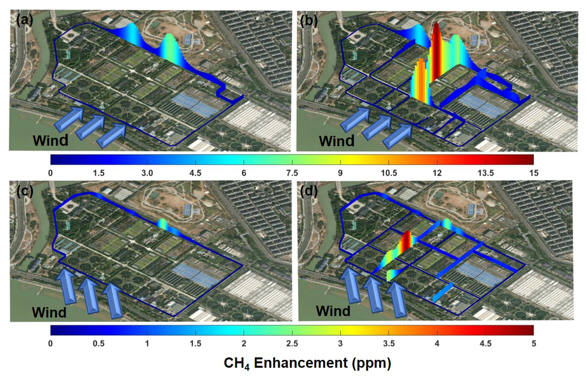
Figure 2 CH₄ concentration maps in the WWTP. The concentration maps for the external roads for 29 June (a) and 13 December (c). The corresponding complete concentration maps that include the internal roads for 29 June (b) and 13 December (d). Map data are from Esri.

The CH₄ concentrations in summer surpass those observed in winter, consistent with a previous study on WWTPs (Masuda et al., 2015). The screen, primary clarifier, and aeration tank are identified as sources with notably higher concentrations. Analysis of concentration distributions reveals that Screen ① shows a peak concentration reaching 14.83 ppm, which is 7.5 times the background concentration. The four primary clarifiers record high concentrations of between 4.79 and 10.88 ppm. The high value of 4.60 ppm measured around the aeration tanks is mainly detected at Aeration Tank ③ . The screen in this study includes coarse and fine screens and a grit chamber, constituting preliminary wastewater treatment to capture larger suspended solids and particulates. The anaerobic environment of the sewer network promotes the production of CH₄ from organic compounds in municipal wastewater. As this wastewater enters the WWTP, the influent contains dissolved CH₄ that originated in the sewer network. During primary treatment, wastewater is elevated through riser mains, facilitating the release of CH₄ into the atmosphere (Guisasola et al., 2008; Bao et al., 2016). The flow velocity, hydraulic design, and detention times in these facilities may affect CH₄ production and release (Alshboul et al., 2016; Yin et al., 2024). The primary clarifier physically removes suspended solids from wastewater through sedimentation, while organic matter undergoes anaerobic microbial degradation, resulting in the substantial production of CH₄ (Masuda et al., 2017). In the aeration tank, operated under anaerobic and anoxic conditions, complex organic compounds are converted to CH₄ by facultative and anaerobic bacteria through biological processes (Yoshida et al., 2014). In contrast, Kupper et al. (2018) identified sludge storage tanks as the primary source of CH₄ emissions in Swiss WWTPs, accounting for 70 % or more of the total emissions. Stadler et al. (2022) monitored CH₄ concentrations inside and around wastewater treatment facilities that ranged from 2.04 to 32.78 ppm, with elevated CH₄ levels predominantly measured near a sludge treatment tank, the digesters, and secondary clarifiers. The CH₄ emissions from various WWTPs are affected by a range of factors, including specific processes, pipeline design, and equipment aging, and mobile monitoring can better reflect the actual emission distribution.

3.2 Emission quantification

The CH₄ concentrations measured via mobile monitoring were employed in combination with the inversion framework to achieve the quantification of CH₄ emissions and localization of the emission sources within the WWTP. Figures 3 and 4 show the locations of identified point sources and the comparison between the measured and simulated concentration distribution. The experiment conducted on 29 June finds Screen ① to be the most significant contributor to CH₄ point source emissions at 18.26 kg h⁻¹, whereas Secondary Clarifier ② is classified as the least significant at 1.23 kg h⁻¹. The correlation coefficient R² for the measured and simulated concentrations is 0.63, with a root-mean-square error (RMSE) of 0.70 mg m⁻³. On 13 December, Aeration Tank ⑤ is the largest point source of CH₄ emissions at 3.93 kg h⁻¹, whereas Primary Clarifier ⑤ is the smallest source at 0.55 kg h⁻¹, with a correlation coefficient R² of 0.70 and an RMSE of 0.28 mg m⁻³. The enhanced correlation between the winter measurement and simulation data, as well as the improved fit of the measurement and simulation value curves, is attributed to the shorter monitoring cycle and more stable meteorological conditions.

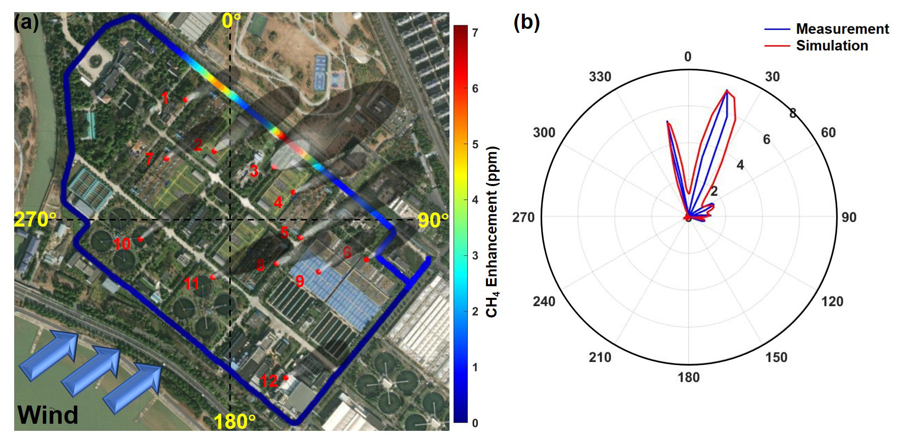
Figure 3 The emission distribution for the source locations (a) and the comparison between measured and simulated CH₄ concentrations (b) at the WWTP on 29 June. Map data are from Esri.

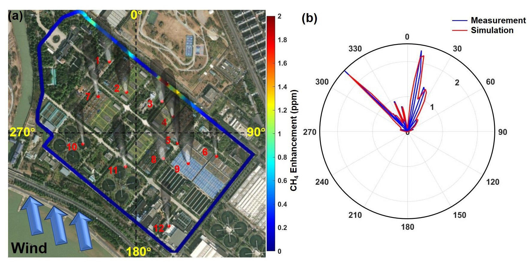
Figure 4 The emission distribution for the source locations (a) and the comparison between measured and simulated CH₄ concentrations (b) at the WWTP on 13 December. Map data are from Esri.

In addition, when employing the multi-source Gaussian diffusion model combined with a genetic algorithm framework for iterative optimization to pinpoint point sources, we were able to locate external sources. As shown in Fig. S2a and c, external sources are primarily located along the main roadway to the south of the WWTP. Moreover, the estimated emissions vary across different days, which indicates that external source emissions are influenced by vehicle traffic. Figure S2b and d compare measured and simulated CH₄ concentrations before and after accounting for external sources, demonstrating that simulations are significantly closer to the measurements when external sources are included.

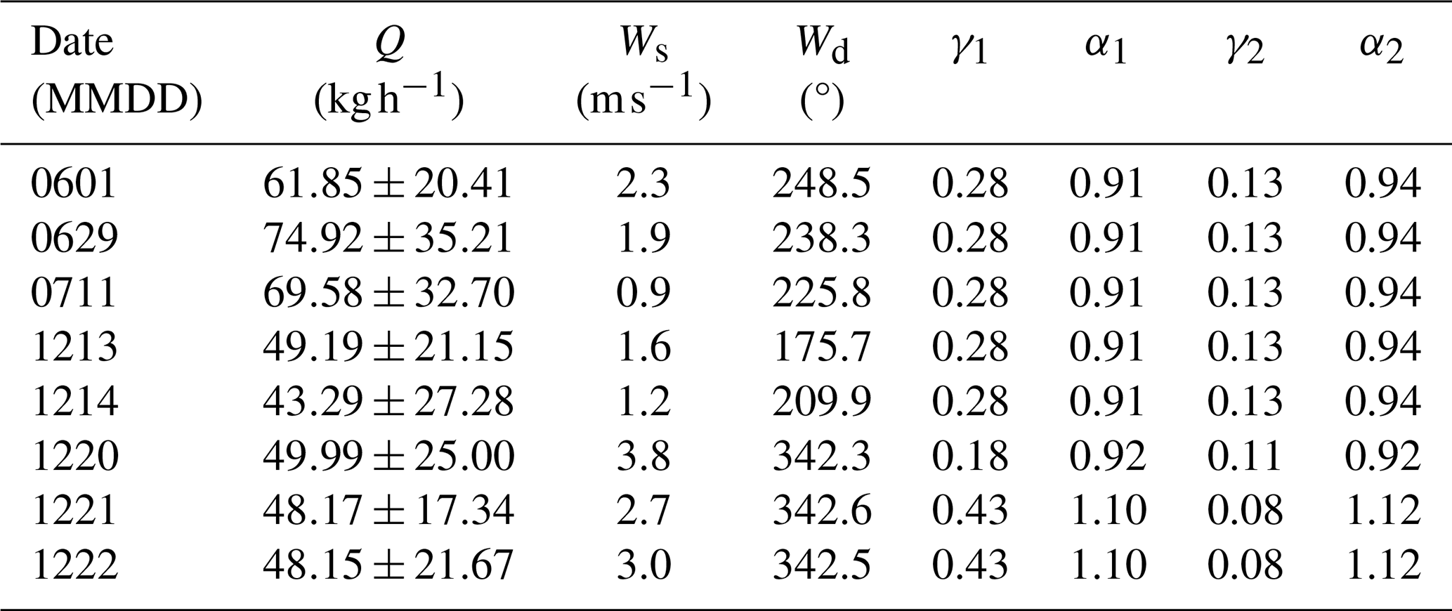
Table 1 displays the CH₄ emission fluxes (Q), wind speed and direction data (W_s and W_d, respectively), the horizontal diffusion coefficient (γ₁, α₁), and the vertical diffusion coefficient (γ₂, α₂) from the 8 d monitoring experiment. Wind speed and direction data are the average wind speed and direction during the monitoring time, and the CH₄ emission fluxes are obtained by the inversion of the average concentration and wind speed and direction data as input to the inversion framework. The emission flux values of CH₄ emission sources (12 point sources and 1 line source) for all experimental days are detailed in Tables S1 and S2 in the Supplement. It is observed that the summer average CH₄ emission flux ($\mathrm{68.78}\pm \mathrm{17.40}\mathrm{kg}{\mathrm{h}}^{-\mathrm{1}}$) surpasses the winter average CH₄ emission flux ($\mathrm{47.76}\pm \mathrm{21.39}\mathrm{kg}{\mathrm{h}}^{-\mathrm{1}}$). This seasonal disparity in emissions is primarily attributed to the aeration tank, followed by the screen and primary clarifier. The activated sludge in the aeration tank contains a higher population of methanogens, whose CH₄ production capability intensifies with rising temperatures (Vítěz et al., 2020). Notably, the seasonal variance in the aeration tank is predominantly driven by the performance of Aeration Tank ④. However, the substantial variation in the emissions from the three summer experiments of Aeration Tank ④ suggests a degree of emission instability. Conversely, the uniformity in the low emissions from the five winter experiments might be associated with the meteorological conditions and the actual operational status of the plant on those days. At lower wind speeds, the CH₄ emissions show only slight differences when compared to emissions on days with higher wind speeds. This suggests that the inversion results are less influenced by wind speed and are primarily associated with seasonal variations.

The screen and primary clarifier are the predominant emission sources at the WWTP. Specifically, these sources emit 37.50 kg h⁻¹ in the summer and 31.92 kg h⁻¹ in the winter, accounting for 55 % and 67 % of the total emissions. Pipeline leaks near the screen and primary clarifier led to the CH₄ release. Previous research has similarly examined major emission sources at WWTPs. Yin et al. (2024) conducted offline monitoring of WWTPs in Beijing and Guiyang, identifying the primary treatment zone as the primary source of CH₄, accounting for 60.1 % and 35.8 % of the respective total emissions. Masuda et al. (2017) analyzed CH₄ emissions from different processes at three WWTPs in Japan, concluding that primary clarifiers are one of the major sources of CH₄ emissions. He et al. (2023) compiled CH₄ emission proportions for different processes in WWTPs based on reported data, finding percentages of 7 %–12 % for the grit chamber, 8.2 %–68.1 % for the primary clarifier, and 18.3 %–86.4 % for the aeration tank.

Table 1 CH₄ emission fluxes (Q), wind speed and direction data (W_s and W_d, respectively), the horizontal diffusion coefficient (γ₁, α₁), and the vertical diffusion coefficient (γ₂, α₂) from the 8 d monitoring experiment.

An alternative top-down approach, known as the tracer gas dispersion method (TDM), has been applied to estimate CH₄ emissions from city streets (von Fischer et al., 2017; Weller et al., 2018), WWTPs (Yoshida et al., 2014; Delre et al., 2017, 2018), biogas plants (Reinelt et al., 2017; Scheutz and Kjeldsen, 2019; Fredenslund et al., 2023), and landfills (Rees-White et al., 2019; Kissas et al., 2022). TDM involves releasing tracer gases like nitrous oxide and acetylene near the source and measuring their concentrations along with CH₄ downwind using a mobile platform. The similar diffusion patterns of CH₄ and the tracer gases result in a stable concentration ratio after atmospheric mixing, enabling the calculation of CH₄ emission rates with a better accuracy (Mønster et al., 2014).

Moreover, TDM was employed to validate and compare other model inversion methods. Moore et al. (2023) proposed that Gaussian dispersion modeling demands less experimental equipment, site access, and personnel than TDM, thereby allowing for swifter data gathering. Yacovitch et al. (2015) utilized a 5 d dataset of tracer gas release in the Barnett Shale region to evaluate the Gaussian dispersion flux quantification method. The results indicated a 95 % confidence interval, with a lower-bound factor of 0.334 and an upper-bound factor of 3.34.The work of von Fischer et al. (2017) presented three controlled release experiments to validate the reliability of a leak rate algorithm in Fort Collins, CO, which indicated a very significant correlation between known and estimated leak rates (p<0.0001, r²=0.43). Compared with the method employed in the study, TDM offers advantages such as simpler formula calculations. Nonetheless, it also presents several drawbacks, including complex experimental procedures and safety hazards associated with the release of tracer gases, which requires access permits from industrial facilities.

3.3 Comparison with the IPCC method

The CH₄ emissions were also calculated using the IPCC method, with data sourced from the Urban Drainage Statistical Yearbook of 2017. The emission flux of $\mathrm{213.95}\pm \mathrm{128.37}\mathrm{t}{\mathrm{a}}^{-\mathrm{1}}$ was determined, with the uncertainty (60 %) derived from the data summarized in the research (Lin et al., 2021). Figure 5 shows the contrast between the emission inversion results from the monitoring experiment and the emission inventory. The uncertainty in the inversion results was determined by accounting for the uncertainties in wind speed, wind direction, and instrument measurements, following the method presented in Sect. 2.4.5. The uncertainties in the emission flux inversion ranged from 33 % to 63 % on individual days. Notably, the uncertainty associated with wind speed contributes approximately 44 %–94 % of the uncertainty range. The summer average inversion emission flux ($\mathrm{603.33}\pm \mathrm{152.66}\mathrm{t}{\mathrm{a}}^{-\mathrm{1}}$) was calculated to be 2.8 times that of the inventory, and the winter average ($\mathrm{418.95}\pm \mathrm{187.59}\mathrm{t}{\mathrm{a}}^{-\mathrm{1}}$) was twice as much. It is posited that the discrepancy may stem from significant uncertainties in the emission factors associated with the WWTPs or the lack of updated activity level data, as the statistical yearbook provided data only up to 2017; therefore, the emission inventory might have underestimated the actual emissions.

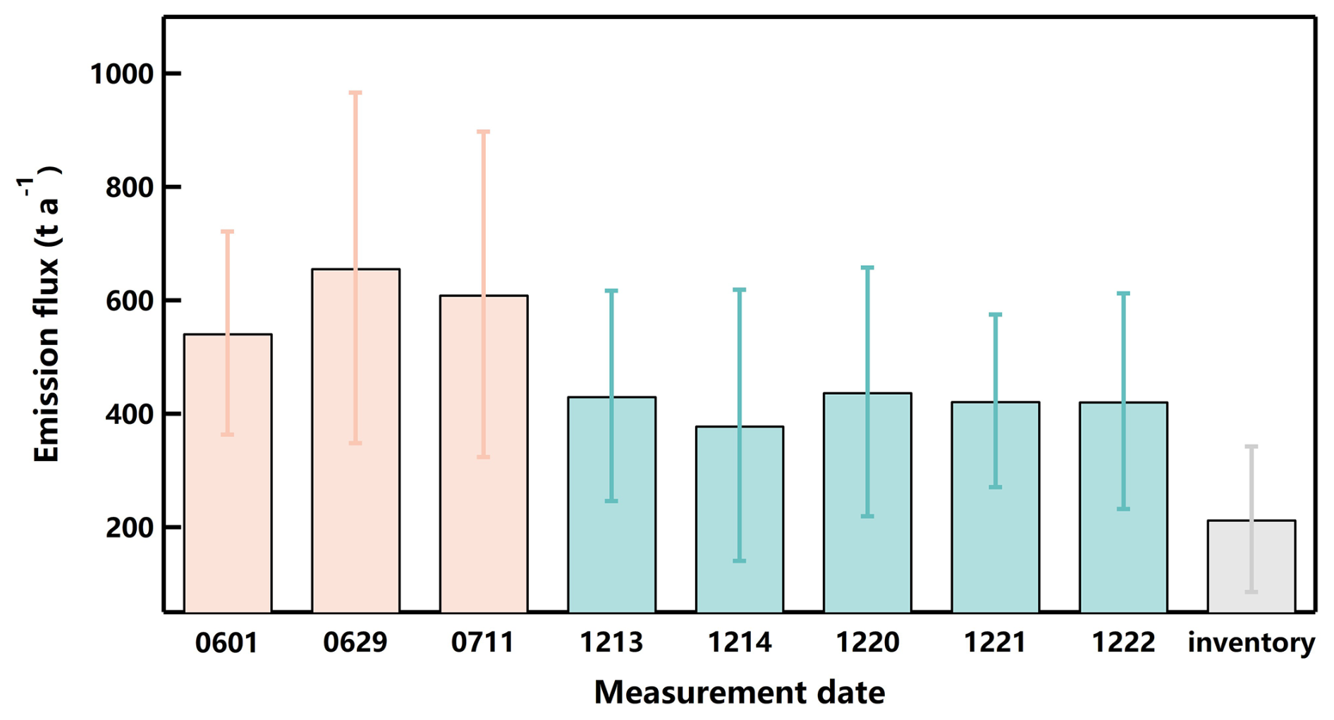
Figure 5 Comparison of CH₄ emission fluxes from the monitoring experiment and emission inventory in the WWTP.

Furthermore, other studies have also investigated the comparison between CH₄ emissions obtained from different measurement methods at WWTPs and the IPCC inventory estimates. The majority of these studies have indicated that the measured values exceed the inventory values. Wang et al. (2021) conducted a measurement-based assessment of CH₄ emissions (46.58 t a⁻¹) in Wuhu City, revealing emission values 46.71 % higher than those calculated using the IPCC method. Moore et al. (2023) employed mobile monitoring to evaluate CH₄ emissions at 63 WWTPs across the USA. Specifically, CH₄ emissions from centrally treated domestic wastewater in the USA amount to $\mathrm{4.64}\times {\mathrm{10}}^{\mathrm{5}}\mathrm{t}{\mathrm{a}}^{-\mathrm{1}}$, which is 1.9 times greater than the Environmental Protection Agency inventory. Song et al. (2023) investigated CH₄ emissions from municipal wastewater treatment in the USA and reported a value of $(\mathrm{4.36}\pm \mathrm{2.8})\times {\mathrm{10}}^{\mathrm{5}}\mathrm{t}{\mathrm{a}}^{-\mathrm{1}}$. This value was approximately twice the estimates provided by the IPCC. Our estimated results are generally consistent with previous studies. The lower estimated results provided by the IPCC method can be attributed to the neglect of certain potential emission sources from the emission inventories, including emissions from equipment in sludge treatment facilities and leaks from pressure relief valves.

3.4 Sensitivity analysis

In this section, we evaluate the stability of the inversion framework through sensitivity analysis and explore the impact of different point source locations on the inversion of emission concentrations. The precise identification of emission sources can enhance the accuracy of emission flux inversion, making a sensitivity analysis of the source location essential. We applied the method of controlling variables to perform a sensitivity analysis on the location of a single point source. The central position of the plant was taken as the reference origin, and the positions of 12 emission sources were determined to analyze the variation in error between measured and simulated concentrations within a 200 m×200 m range around each emission source. We sequentially modified the source position parameters in the model input to analyze the congruence between the simulated concentrations and the observed measurements, quantifying the fit using the RMSE. The change in concentration error serves as an indicator of the accuracy of the emission source localization.

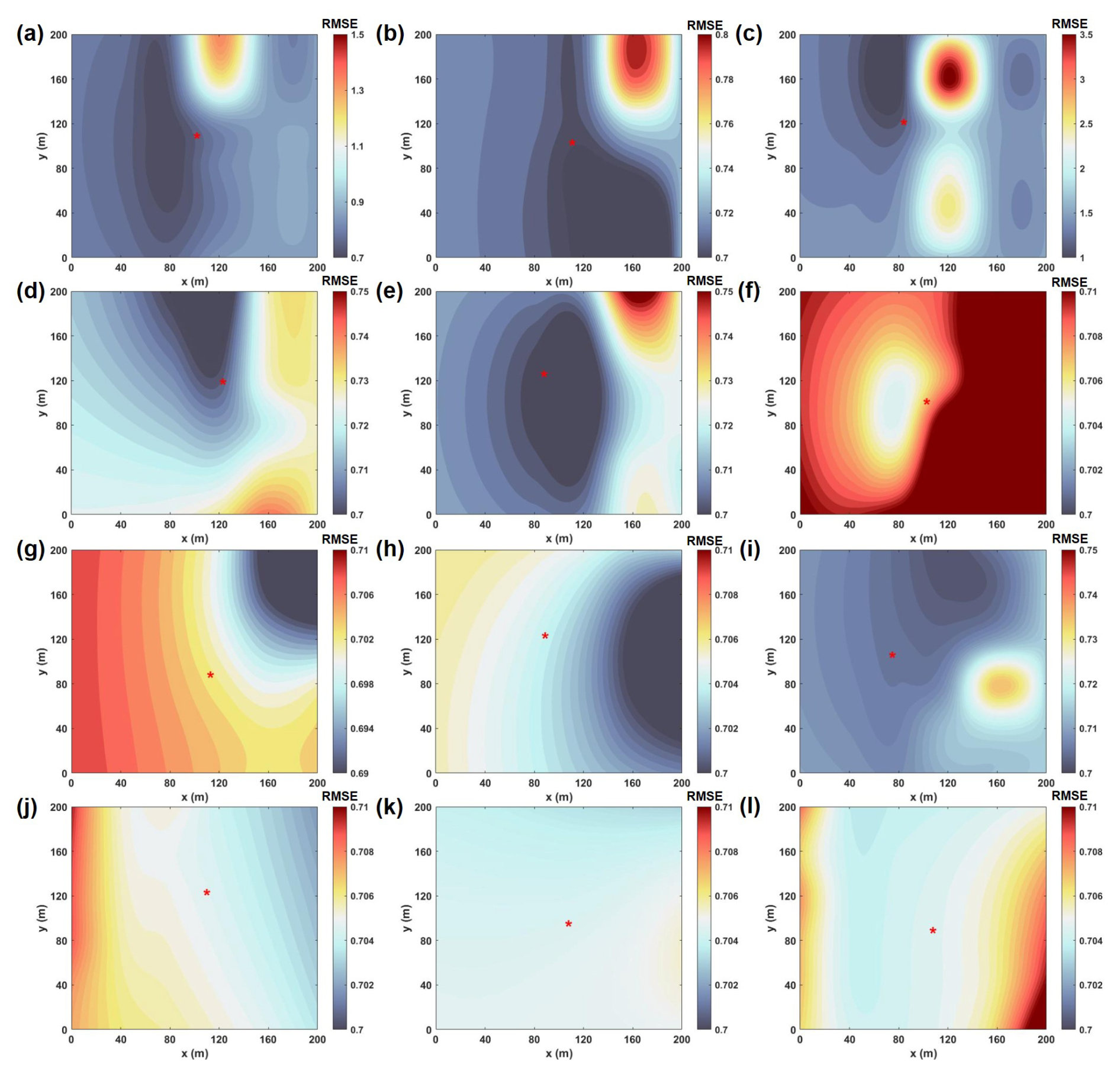
Figure 6 The root-mean-square error (RMSE) of the simulated concentration changes with the location of the WWTP source on 29 June. The x and y axes denote the respective horizontal and vertical distances of the simulated point source from the central point of the WWTP. The variation in color signifies the alteration in the RMSE between the actual monitored and simulated concentrations, with the red star symbolizing the simulated point source location.

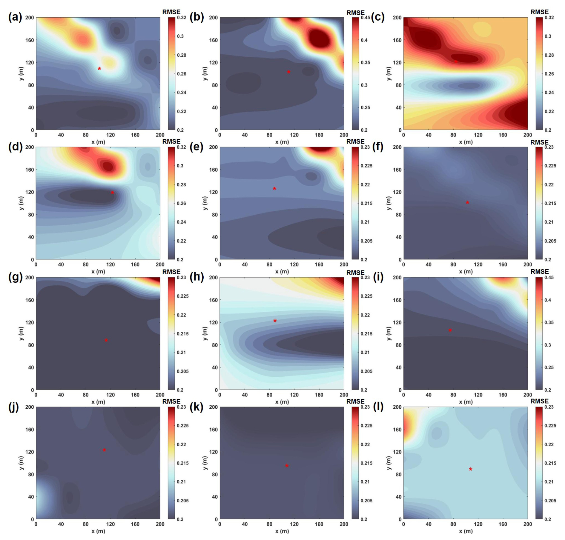
Figure 7 The RMSE of monitoring simulated concentration changes with the location of the WWTP source on 13 December.

Figures 6 and 7 describe the error variation between monitored and simulated concentrations when the point source location is subject to change within a 200 m×200 m range from the monitoring experiment on 29 June and 13 December. The error variation in the remaining days can be seen in Figs. S9–S14. The point source locations simulated based on the inversion framework are mostly in areas with minor relative concentration errors, which can be considered to have a high reliability in simulating point source locations. The emission source location errors for the two experiments are within the ranges of 0.7–1.3 and 0.2–0.3 mg m⁻³. The winter emission source locations exhibit greater stability and accuracy in the inversion results than the summer ones.

4 Conclusions and outlook

This study carried out mobile measurements at a WWTP in Hangzhou across the summer and winter seasons of 2023. By employing a multi-source Gaussian plume model combined with a genetic algorithm inversion framework, the inversion of CH₄ emission fluxes and their source locations was achieved. The results showed that 12 distinct CH₄ emission sources were pinpointed. The average CH₄ emission flux during the summer was $\mathrm{68.78}\pm \mathrm{17.40}\mathrm{kg}{\mathrm{h}}^{-\mathrm{1}}$ ($\mathrm{603.33}\pm \mathrm{152.66}\mathrm{t}{\mathrm{a}}^{-\mathrm{1}}$), whereas this value was $\mathrm{47.76}\pm \mathrm{21.39}\mathrm{kg}{\mathrm{h}}^{-\mathrm{1}}$ ($\mathrm{418.95}\pm \mathrm{187.59}\mathrm{t}{\mathrm{a}}^{-\mathrm{1}}$) during winter. The screen and primary clarifier were the main sources, accounting for 55 % of summer and 67 % of winter emissions. The summer CH₄ inversion emissions were found to be 2.8 times higher, and the winter inversion emissions were twice as high as the inventory-based estimation.

The inversion framework is capable of validating emission coefficients in the inventory, identifying emission sources within the plant, and monitoring abnormal emissions. It can be applied to various monitoring systems, such as UAV systems and networks of fixed monitoring stations. We believe that this collaborative monitoring offers significant improvements with respect to the accuracy of emission fluxes and source inversion. Future efforts should aim to refine the inversion framework for broader applicability to various pollutant gases, enhancing the inversion efficiency, and extending the validation of the framework through monitoring experiments in a diverse range of industrial facilities.