Measurement report: Greenhouse gas profiles and age of air from the 2021 HEMERA-TWIN balloon launch

Within the HEMERA balloon infrastructure project, a stratospheric balloon carrying a multi-instrument payload to a maximum altitude of 31.2 km was launched on 12 August 2021. On board the openly constructed gondola, several types of instruments were used for simultaneous air sampling and in-flight measurements to characterize climate-relevant trace gases in the stratosphere and troposphere, as well as to compare and evaluate different instrumental approaches and sampling techniques. For observations of the main greenhouse gases carbon dioxide (CO₂), methane (CH₄), nitrous oxide (N₂O), and sulfur hexafluoride (SF₆), flask with AirCore sampling and in-flight spectrometry were deployed. Overall, results from different methods agree well. While better precision was achieved for the post-flight measurements of AirCore devices and flask sampling, in situ spectrometry provided a higher degree of detail on the vertical structure of the CH₄ profile. Age of air was derived from mixing ratios of CO₂ and SF₆. As seen in previous studies, higher values were obtained from SF₆ than from CO₂. Correcting for chemical losses, maximum values of 4.4–5.1 years were derived from SF₆ mixing ratios at altitudes above 20 km compared to 4.2–5.0 years from CO₂ mixing ratios. The resulting dataset should be well suited for multi-tracer approaches to derive age of air, particularly in combination with a large suite of halocarbons measured from flask and AirCore sampling and one more AirCore sample which was reported in a companion publication (Laube et al., 2025).

1 Introduction

High-altitude balloons continue to be the only means for in situ observations of chemical composition at altitudes that cannot be reached by aircraft, i.e. above ca. 20 km. Lightweight instrumentation, such as ozone sondes, can be lifted with small weather balloons that can be launched routinely. Many trace gases, however, can only be measured with more complex instruments or from sampled air analysed post-flight in the laboratory (Ehhalt, 1980; Fabian, 1981). Cryogenic air sampling is an established method for the efficient collection of air samples in the stratosphere (Ehhalt, 1974; Lueb et al., 1975; Schmidt et al., 1984, 1987) to obtain observations of trace gas profiles from the stratosphere.

Such data are, for example, relevant to constrain potential changes in stratospheric circulation induced by climate change (Austin and Li, 2006; Engel et al., 2009; Stiller et al., 2012; Eichinger et al., 2019; Abalos et al., 2021). It is also of interest to perform measurements of ozone-depleting gases directly at the altitudes where ozone depletion occurs (Ray et al., 2002; Brinckmann et al., 2012; Krysztofiak et al., 2023). For substances which are measurable with remote-sensing methods, data from balloon-borne air samples can also be used for satellite retrieval validation or to validate ground-based measurement networks such as the Total Carbon Column Observing Network (TCCON) and the Network for the Detection of Atmospheric Composition Change (NDACC), deploying Fourier transform infrared spectrometers (Zhou et al., 2018). This was, for example, recently demonstrated for vertical profiles of HCFC-22 (chlorodifluoromethane, CHClF₂) measured by the ACE-FTS satellite instrument (Kolonjari et al., 2024) using data from the analysis of flasks sampled at ground-based sites, on board aircraft, and during four earlier flights of the identical cryosampler used for the HEMERA-TWIN launch. However, due to the high costs and safety aspects of such launches, profiles from large high-altitude balloons remain sparse in their spatial and temporal coverage (Krysztofiak et al., 2023; Ray et al., 2024).

Over the last decade, air sampling with AirCore, based on an idea initially proposed by Tans (2009), has been established as a method for measurements of vertical profiles of CO₂ and CH₄ (Karion et al., 2010; Membrive et al., 2017; Engel et al., 2017; Wagenhäuser et al., 2021). AirCore devices are lightweight air sampling tools based on stainless-steel tubes that are open at one end and closed at the other. Making use of the pressure changes with altitude, air is passively sampled into the tube during the descent from high altitudes to the ground. They are often sufficiently lightweight to be carried by small weather balloons. This approach is complementary to classical flask sample collection at distinct altitudes. While the latter averages over a few well-defined sampling intervals, AirCore samples represent a continuous profile. AirCore samples need to be analysed quickly after sampling to minimize the averaging effects of molecular diffusion within the sample tube and to achieve the best possible vertical resolution. Also, sub-sampling of AirCore samples for later analysis using discontinuous analytical methods – at the expense of losing altitude resolution – is possible (Laube et al., 2020). Sub-sampled AirCore samples, as with original flask samples, can be analysed for many species, even after longer times of storage, depending on the chemical stability of compounds in the flasks. The 2021 launch of the HEMERA-TWIN gondola described in this measurement report allowed for the simultaneous deployment of several AirCore packages for intercomparison of different AirCore set-ups and for comparison with other measurement methods, which is not possible with small weather balloons because of their payload weight restrictions.

To investigate stratospheric transport timescales, the concept of mean age of air has proven to be a useful tool. As the stratospheric circulation cannot be observed directly, a quantity that can be derived from observations of trace gas mixing ratios is needed to characterize stratospheric transport. Mean age of air can be used to diagnose the current overall strength of the large-scale Brewer–Dobson circulation but also allows us to investigate changes that might be a consequence of climate change (Hall and Plumb, 1994; Waugh and Hall, 2002; Engel et al., 2009; Garny et al., 2024b).

Commonly, the mean age of air is interpreted as the mean transit time that it took for all contributions to an observed air parcel to arrive at the observation location from their respective entry points into the stratosphere. The calculation relies on a reference time series of mixing ratios measured at a reference surface. Often, the tropical tropopause is chosen as the reference surface. For the lower stratosphere of the midlatitudes, more sophisticated approaches take into account cross-tropopause transport in the extra-tropics as well (Hauck et al., 2020; Wagenhäuser et al., 2023; Ray et al., 2024). Generally, the stratospheric age of air can be calculated from observations of long-lived trace gases which have a monotonous trend in the troposphere, e.g. SF₆ or, when de-seasonalized, CO₂ (Engel et al., 2002, 2017; Bönisch et al., 2009; Garny et al., 2024a; Ray et al., 2014, 2024). Also, halocarbons have been used to derive age of air (Daniel et al., 1996; Volk et al., 1997; Harnisch et al., 1999; Leedham Elvidge et al., 2018). Age-of-air values need to be corrected for the acceleration of tropospheric trends, as trace gas mixing ratios in general show non-linear trends (Plumb and Ko, 1992; Volk et al., 1997; Engel et al., 2002). In addition, the chemical sinks of SF₆ may introduce significant biases to the calculation (Stiller et al., 2012; Ray et al., 2017; Kovács et al., 2017; Leedham Elvidge et al., 2018). Recently, Garny et al. (2024a) proposed a model-based correction scheme to account for chemical sinks of SF₆. For CO₂, the seasonal cycle in the troposphere also needs to be taken into account at least in the lower stratosphere (Bönisch et al., 2009; Andrews et al., 2001; Diallo et al., 2017).

Here, we report on the HEMERA-TWIN balloon launch of 2021 which aimed at sampling and analysing stratospheric air to measure atmospheric trace gases using four types of instruments: in situ spectrometric analysis, cryogenic air sample collection in stainless-steel canisters, and bag and AirCore sampling. This combination of instruments allows researchers to compare vertical profiles of the long-lived greenhouse gases CO₂, CH₄, SF₆, and N₂O measured at different altitude resolutions and of the mean age of air derived from SF₆ and CO₂. As discussed in our companion paper, the collection of air samples provides additional data on mixing ratios of halocarbons, many of them being strong greenhouse gases and ozone-depleting substances (Laube et al., 2025).

2 Methodology

2.1 The HEMERA-TWIN balloon launch

HEMERA is a balloon infrastructure project offering balloon flights for research and innovation. It is funded by the European Commission within the Horizon 2020 programme and is coordinated by the French space agency CNES (Centre National d'Etudes Spatiales). In August 2021, the openly constructed TWIN gondola, shown in Fig. 1, was used as part of the HEMERA flight programme to carry a suite of instruments to measure the vertical distribution of several long-lived greenhouse gases and ozone-depleting substances. The TWIN gondola, with its name referring to the symmetric frame structure, has been used before in similar studies and is considered to be suited for whole-air sampling without contamination of the sampled air (Engel and Schmidt, 1994). The open structure avoids contact of the sampled air with surfaces and thus reduces the probability of contamination.

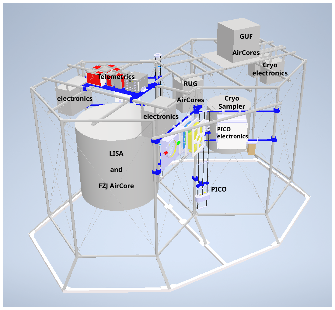
Figure 1 Layout of the TWIN gondola for the HEMERA 2021 launch. The gondola height is 2.2 m, the footprint is 2.6 m × 4 m, and the total weight including the instrumentation amounts to approximately 345 kg. Its name (TWIN) refers to the symmetric structure of the gondola frame.

The launch took place on 12 August 2021 at 21:18 UTC from the European Space and Sounding Rocket Range (Esrange) in Kiruna, Sweden (located 68° N, 21° E), at approximately 330 $\mathrm{m}\mathrm{a}.\mathrm{s}.\mathrm{l}.$ altitude. Ascent took place over approximately 3 h and 45 min at an average altitude rate of 4.5 m s⁻¹, and the balloon reached a maximum altitude of 31.2 km around 23:12 UTC, where it spent approximately 7 min, before descent started. The valve-controlled slow descent was over approximately 3 h and 50 min with an average vertical speed of −1.5 m s⁻¹ between 31 and 13 km and an average vertical speed of −8.2 m s⁻¹ below 13 km after separation of the gondola from the main balloon. Touchdown was at 03:02 UTC. All sampling of air was during the descent to avoid possible contamination of sampled air by the balloon or the gondola itself. The height of the tropopause was derived from radiosonde data during the balloon ascent by calculating the slope of the temperature profile. The tropopause height has been assigned at 10.5 km where the temperature change with altitude first reached the value of 2 K km⁻¹, following the World Meteorological Organization (WMO) definition.

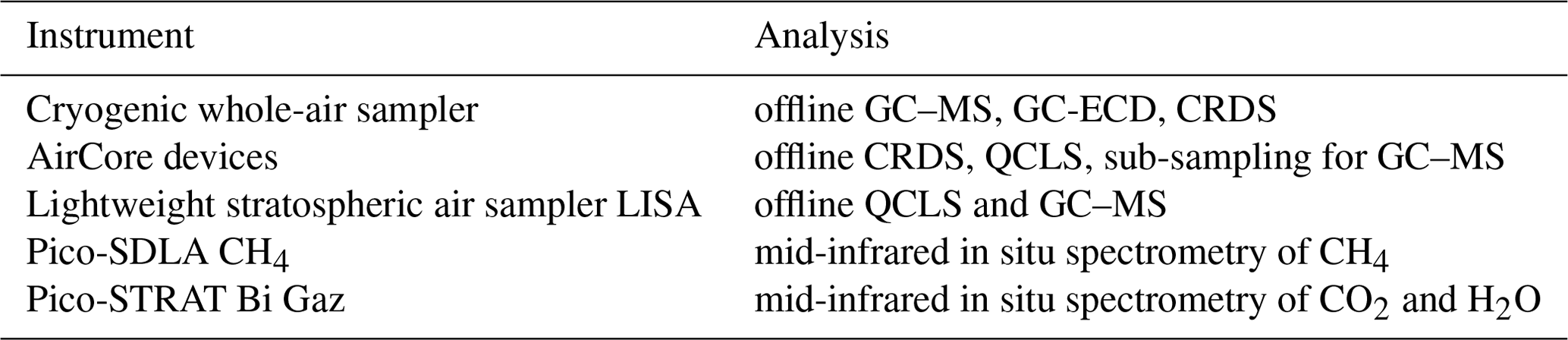
The individual instruments of the payload are listed in Table 1, and Fig. 1 shows the layout of the payload within the gondola structure. The gondola is 2.2 m in height over a base area of 2.6 m × 4 m. In summary, the balloon carried the cryogenic whole-air sampler (Schmidt et al., 1987), five different AirCore set-ups (Engel et al., 2017; Wagenhäuser et al., 2021; Laube et al., 2025), and two mid-infrared diode laser spectrometers (Pico-SDLA CH₄ and Pico-STRAT Bi Gaz) for in situ measurements of CH₄ and CO₂ (Ghysels et al., 2011, 2014).

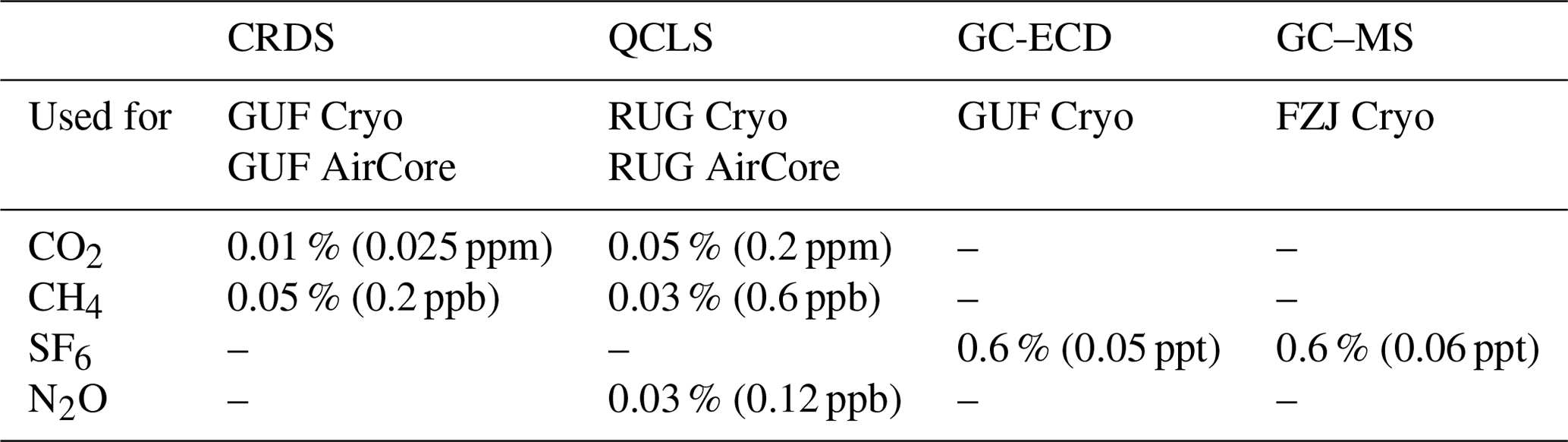
Table 1 The payload of the HEMERA-TWIN gondola on 12 August 2021. AirCore samples and air samples were analysed post-flight with quantum-cascade laser spectroscopy (QCLS), cavity ring-down spectroscopy (CRDS), and gas chromatography (GC) coupled with an electron capture detector (ECD) or a mass spectrometer (MS), whereas Pico-SDLA CH₄ and Pico-STRAT Bi Gaz are in situ instruments measuring in flight.

Position data as well as ambient pressure and temperature were recorded by the Pico-STRAT Bi Gaz instrument. The position data include GPS altitude and latitude and longitude from a global navigation satellite system (GNSS). Pressure measurements were performed with a ParoScientific Inc. absolute gauge, and ambient temperature values were recorded by three fast-response temperature sensors (Sippican).

In addition, the payload included a newly constructed air sampler for the collection of large air samples in foil bags, which was developed based on the LIghtweight Stratospheric Air sampler (LISA) (Hooghiem et al., 2018). This sampler will be described in a separate publication, and data are not included here. The total weight of the payload was approximately 345 kg.

In the post-flight analyses of flask and AirCore samples, mixing ratios were measured as follows: CO₂ on the WMO X2019 scale (Hall et al., 2021), CH₄ on the WMO X2004A scale (Dlugokencky et al., 2005), and N₂O on the WMO X2006A scale (Hall et al., 2007). SF₆ mixing ratios are reported on the WMO X2014 scale (NOAA, 2014).

2.2 The Pico-SDLA spectrometers

Pico is a balloon-borne spectrometer developed to probe vertical profiles of atmospheric CH₄ and CO₂ (Ghysels et al., 2011, 2014). During the HEMERA-TWIN flight, two Pico instruments were launched: Pico-SDLA CH₄ and Pico-STRAT Bi Gaz (${\mathrm{H}}_{\mathrm{2}}\mathrm{O}/{\mathrm{CO}}_{\mathrm{2}}$). The Pico-STRAT Bi Gaz (bi gaz: dual-gas in French) spectrometer is an evolution of the former Pico-SDLA instruments to suit long-duration observations. This adaptation has been initiated within the STRATeole 2 balloon-borne project. (Carbone et al., 2024). The Pico-SDLA CH₄ instrument performed well, whereas Pico-STRAT Bi Gaz measurements suffered from undesired electromagnetic interference for which the source remains undetermined, resulting in spectrum deformations for CO₂. Therefore, CO₂ measurements are unusable for this flight.

Pico-SDLA CH₄ deploys a mid-infrared distributed-feedback laser emitting at 3.24 µm. The laser beam is propagated in the open atmosphere over a total absorption path length of ∼3.6 m after multiple reflections. The total weight of the device is approximately 8.5 kg. The simple and robust design of the optical cell minimizes mechanical vibrations, thereby limiting variations in the spectrum baseline. Pico-SDLA CH₄ was integrated into the gondola in a vertical position. The slow ascent and descent reduced mechanical vibrations, thereby increasing the optical cell instrumental stability.

The wavelength of the laser emission is tuned by ramping the laser driving current every 10 ms. Atmospheric mixing ratios are retrieved from the in situ absorption spectra using a molecular model in conjunction with in situ atmospheric pressure and temperature measurements. Ambient pressure is measured by an absolute pressure transducer with 0.01 % accuracy (ParoScientific Inc.), and measurements are averaged over 0.5 s. Ambient temperature is measured using three fast-response temperature sensors (Sippican) with an uncertainty of 0.2 °C and a resolution of 0.1 °C on the temperature reading. Measurements are averaged over 1 ms with outliers removed. Sensors are located at each end of the optical cell and at its centre. The sensors are known to be susceptible to solar and infrared radiation, but no correction was necessary as measurements took place during the night. The temperature uncertainty was improved by an intercomparison programme (Oakley et al., 2011).

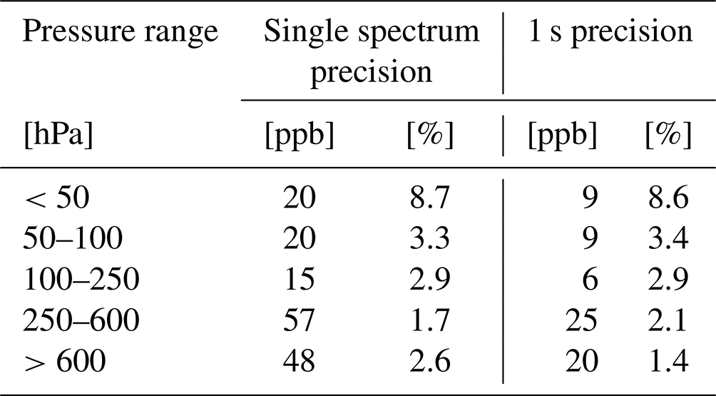
The noise of one spectrum is about $\mathrm{4}\times {\mathrm{10}}^{-\mathrm{4}}$ in absorption units. Using single spectra, the measurement precision scales from 48 ppb at the ground down to 15 ppb around the tropopause. For a 1 s averaging time, the precision varies from 25 ppb in the troposphere down to 6 ppb in the upper troposphere and lower stratosphere (UTLS) (see Table 2). Spectroscopic laboratory work has been conducted in order to determine the appropriate molecular model, accounting for temperature-related effects (Ghysels et al., 2014). This improved the measurement accuracy. The uncertainty budget includes the uncertainty due to the frequency axis and baseline interpolation, the uncertainty due to experimental noise and spectroscopy, and the uncertainties of pressure and temperature. Table 2 lists the measurement uncertainties of Pico-SDLA CH₄ from the ground up to the balloon ceiling.

Table 2 Uncertainties of Pico-SDLA CH₄ measurements obtained in flight as a function of pressure level.

2.3 Vertical profile measurements with AirCore

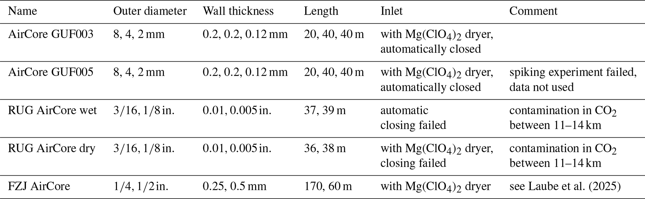
The gondola carried three different AirCore packages: from Goethe University Frankfurt (GUF), from the University of Groningen (Rijksuniversiteit Groningen, RUG), and from Forschungszentrum Jülich (FZJ). An overview is given in Table 3.

Laube et al. (2025)

Table 3 Properties of the five different AirCore devices in the payload.

The AirCore sampling system is based on a concept first presented by Karion et al. (2010) from an idea originally developed and patented by Tans (2009). AirCore set-ups consist of long and narrow stainless-steel tubing which at launch time is closed at one end and open at the other. Prior to launch, the AirCore is filled with a gas of well-known composition. It evacuates due to decreasing ambient pressure during ascent and reversely samples ambient air with increasing pressure during descent. To avoid loss of sample air or contamination, AirCore tubes may be equipped with a mechanism to automatically close the tube upon landing. After recovery, the sample is analysed for trace gas mixing ratios with a continuous-flow gas analyser, and the resulting measurements are attributed to the sampling altitudes. Altitude attribution was based on pressure readings from the Pico-SDLA CH₄ instrument for both the GUF and RUG AirCore devices. To attribute the measured trace gas mixing ratios to sampling altitude, the pressure- and temperature-dependent amount of sampled air is calculated as a function of altitude and related to the amount of sample air measured at a constant flow as a function of measurement time. A small amount of fill gas remains in the AirCore tube, which during descent is pushed towards the closed end of the AirCore. During analysis, which is performed in the reverse direction, the remaining fill gas marks the start of the AirCore sample in the measurement time series. In this procedure, an easily distinguishable fill gas facilitates the analysis.

Including electronics, AirCore set-ups from GUF and RUG each add only 3 kg to the payload, which in a single instrument package makes them deployable with small weather balloons. Deploying them as part of a large instrument package allows for the comparison of different configurations. Another larger AirCore, developed and operated by FZJ, was sub-sampled for laboratory GC–MS analysis of halogenated tracers (Laube et al., 2020). Results thereof are discussed jointly with the GC–MS results from the cryogenic whole-air sampler in a companion paper (Laube et al., 2025).

For GUF, the main scientific objective of AirCore measurements is the determination of the mean age of air from CO₂. Therefore, the AirCore tubes are geometrically designed such that the highest vertical resolution is obtained for the stratosphere (Membrive et al., 2017). They are composed of three different sections with smaller diameters towards the stratospheric end to reduce mixing due to diffusion during the time between sampling and measurement (inner diameters: 7.6, 3.6, and 1.76 mm; outer diameters: 8, 4, and 2 mm; length: 20, 40, and 40 m). Further details have been described by Engel et al. (2017) and Wagenhäuser et al. (2021). The AirCore tubes are constructed from custom-made stainless-steel tubing which has been silanized, as suggested by Karion et al. (2010), using Silconert2000^® to reduce wall effects and to enhance sample stability during storage. Both AirCore set-ups were equipped with Mg(ClO₄)₂ dryers at the inlet and were automatically closed upon landing.

For the 2021 TWIN gondola launch, one GUF AirCore was equipped with a CO-spiking experiment as described by Wagenhäuser et al. (2021) to test the altitude attribution. Because the spiking experiment failed, only results of the AirCore with default configuration are presented here. The initial fill gas of both GUF AirCore tubes had CH₄ and CO₂ mixing ratios close to those expected in the middle stratosphere but was spiked with CO, resulting in a CO mixing ratio of 1436.41 ppb. Mixing with the remaining fill gas is taken into account during the retrieval as described by Wagenhäuser et al. (2021). Thus, the uppermost part of the AirCore profile can be used for scientific evaluation as well.

Starting ∼3 h after landing, GUF AirCore samples were analysed for CO, CH₄, CO₂, and H₂O using a Picarro G2401 CRDS, and results are reported as dry mixing ratios. The measurement data are calibrated in two steps. First, the raw data were processed with instrument-specific parameters that are valid over the long term. Therefore, a linear calibration curve for each component using analyser-specific slope and offset values was applied. These device characteristics were determined in laboratory experiments prior to the campaign. Secondly, the values were corrected for instrumental drift with a day-specific offset determined by measuring a calibration gas tank immediately after the AirCore analysis.

Altitude attribution was performed as described by Engel et al. (2017) and Wagenhäuser et al. (2021). The start and end points of the AirCore sample in the measurement time series were determined using the known mixing ratios of the remaining fill gas that the AirCore tube is filled with prior to the launch and the push gas that is used to push the sample air towards the Picarro instrument during the post-flight analysis. The vertical resolution of the GUF AirCore devices ranges from about 1000 m at 25 km to better than 300 m around the tropopause and in the troposphere. However, the geometry of the AirCore plays a central role in this uncertainty, so the three individual sections of the GUF AirCore with their different internal diameters and lengths must be taken into account. At lower altitudes, the effect of molecular diffusion on the vertical resolution is larger because of the wider tube diameter. At the top of the profile, mixing in the analyser cell during post-flight analysis is the dominating effect. Further details on the AirCore data analysis including the altitude attribution and fill gas correction were reported by Wagenhäuser et al. (2021).

The RUG AirCore set-ups are similarly designed with smaller diameters towards the stratospheric end to reduce mixing during sampling and sample recovery, each consisting of two sections of different diameters: outer diameters of $\mathrm{3}/\mathrm{16}$ and $\mathrm{1}/\mathrm{8}\mathrm{in}.$ with wall thicknesses of ∼0.01 and $\sim \mathrm{0.005}\mathrm{in}.$ and lengths of 37 and 39 m for one AirCore and 36 and 38 m for the other. The sections were connected with an externally glued union piece. One AirCore's inlet was equipped with a Mg(ClO₄)₂ dryer, while the other AirCore's inlet was left open to investigate possible water effects on the retrieved profiles. After landing and retrieval, both AirCore samples were measured on a dual-laser Aerodyne QCLS, detailed below in Sect. 2.5 and in Vinković et al. (2022) and Tong et al. (2023). The altitude attribution was realized following the approach described in Membrive et al. (2017).

Unfortunately, in both AirCore tubes, the glued connector caused a contamination issue for CO₂ between 11–14 km of altitude. The affected data in this range are not reported and are visible as gaps in the profiles. Upon landing, the closing mechanism of both RUG AirCore set-ups malfunctioned, likely due to prolonged cold exposure during the flight. The closing attempt drained the batteries, shutting down the data loggers, and no temperatures were recorded. Warming of the open-ended tubing between landing (03:02 UTC; $T\sim -\mathrm{45}$ °C) and capping by the recovery team (approximately 04:15 UTC; T unknown) will have led to a loss of sample from the RUG AirCore samples, which consequently will have led to an altitude attribution of the profile that is too low. The exact loss and attribution bias cannot be stated with certainty as no temperature data for a volumetric correction were recorded. Indicatively, heating by 10 °C would lead to a low bias in altitude attribution of ∼300 m in the lower troposphere, while the stratospheric part of the profile would be less affected.

Additional uncertainty exists for the stratospheric measurements and altitude attribution: the top and bottom of the retrieved profiles are biased by mixing with the remaining fill gas and the gas employed to push the AirCore air in the instrument. Given uncertainties regarding the gas composition and the actual mixing fractions of the profiles and fill/push gases over the analysis time, the upper and lower parts of the RUG profiles are not reported.

2.4 Cryogenic whole-air sampling

The cryogenic whole-air sampler holds 15 stainless-steel sample flasks with volumes of 0.58 L (five flasks) or 0.31 L (10 flasks), which were evacuated before the launch. Each flask has an individual inlet system, made of metal and glass, which is opened and closed interactively through telemetry commands from the ground. Inlet lines open towards the bottom of the sampler to avoid contact of the sampled air with any equipment. During sampling, ambient air is cryogenically trapped with liquid neon. The air sampler contains a 10 L reservoir of liquid neon which is filled prior to launch. Further details on the sampler were described by Schmidt et al. (1987). During the HEMERA 2021 launch, the five larger sample flasks were equipped with cotton filters to scrub ozone for accurate measurements of carbonyl sulfide (COS), replacing manganese dioxide on glass wool previously used for this purpose (Andreae et al., 1985; Hofmann et al., 1992; Persson and Leck, 1994; Engel and Schmidt, 1994).

In total, 14 samples were successfully collected during descent at altitudes ranging from 30.8 down to 13.5 km; final sample pressures ranged from 8 to 33 bar, corresponding to a total sample volume of 4.6–19.1 L STP (standard temperature and pressure). The sample time varied between 43 and 731 s, corresponding to an altitude range of 85–1278 m, depending on the respective descent velocity. Different types of post-flight analyses of the sampled air were performed at laboratories at GUF, RUG, and FZJ.

2.5 Air sample analysis

All flasks of the cryosampler were analysed at GUF with GC–MS for halocarbons; with gas chromatography coupled with electron capture detection (GC-ECD) for CFC-12 and SF₆; and with continuous-flow CRDS also used for AirCore analysis of CO₂, CH₄, and CO. The sample volumes used for these analyses were two times 1 L for GC–MS and approximately 0.27 and 0.11 L for GC-ECD and CRDS analyses, respectively. The cryosampler was then transferred to RUG, where the continuous-flow QCLS used for AirCore analysis was deployed to measure CO₂, CH₄, and N₂O from the sample flasks. This used approximately 0.25 L of sample volume. Lastly, samples were analysed for SF₆ at FZJ using a GC–MS set-up that needs 0.25 L of sample volume.

At GUF, all flask samples were analysed for halogenated compounds with a GC–MS set-up almost identical to the one described by Hoker et al. (2015) and Schuck et al. (2018) but deploying a quadrupole mass spectrometer in selected ion monitoring mode only. In addition, the air samples were analysed with a semicontinuous GC-ECD set-up for CFC-12 and SF₆ (Engel et al., 2006; Jesswein et al., 2021; Wagenhäuser et al., 2023) and by high-resolution CRDS, deploying the instrument described in Sect. 2.3 for analysis of CO₂, CH₄, and CO. Because CO is known to form in the stainless-steel canisters (Novelli et al., 1992), only CO₂ and CH₄ data are presented. SF₆ data from the GC-ECD instrument are measured on the SIO-05 scale, and a conversion factor of 1.0049±0.002 was applied to convert to the WMO X2014 scale (Prinn et al., 2018). One sample, collected without cotton scrubber at 19.3 km altitude, was excluded from further analysis for CO₂ and CH₄ due to an unrealistically high mixing ratio of COS above 5 ppb as detected during GC–MS analysis and a CO₂ mixing ratio above 420 ppm. These high values might indicate a stability issue during storage. Mixing ratios of SF₆ and N₂O are shown, as these compounds are chemically inert and unlikely to be affected by storage effects. Furthermore, a sample equipped with cotton scrubber collected at 17.9 km altitude was excluded because unrealistically high mixing ratios of several trace gases were measured, including CO₂, SF₆, and several halogenated compounds, which points to a contamination of this sample. All measurements of halogenated tracers with the GC–MS set-up from the cryogenic air samples will be presented in a companion paper (Laube et al., 2025).

At RUG, in September of 2021, the cryosamples were analysed on a quantum-cascade laser spectrometer (QCLS; model TILDAS Dual, Aerodyne Research Inc., MA, USA). Its first laser (scan centred around wavenumber 1275.5) observes CH₄, N₂O, and H₂O, while its second laser (around wavenumber 2050.6) observes COS, CO₂, and CO. The cavity of the analyser is maintained at a pressure of 50 ± 0.002 Torr (∼66 hPa) and a temperature of 250 ± 0.002 °C. Under these conditions, the equivalent volume of the optical cavity is ∼10 cm³ (geometric volume ∼150 cm³), and a precision better than 0.6, 0.12 ppb, and 0.20 ppm is attained for CH₄, N₂O, or CO₂, respectively (1σ of individual samples, collected at 1 Hz). The sample flow rate is ∼50 sccm (standard cubic centimetre per minute).

The instrument stabilization is of a “double-exponential” character, i.e. exhibiting an initially rapid approach to the final value but then taking a long time to become stable. This depends on species and is more pronounced for CO₂ than for CH₄. The measurement duration of ∼5 min, chosen to conserve precious sample, does not, for all samples, result in quantitative replacement of the previous sample. In order to maximize the value of our analysis, a double-exponential function was fit to the measurement data and used to predict the true sample value, i.e. the asymptote of the function. The deviations between the asymptote and the mean of the last 60 s of a sample were for almost all samples smaller than the uncertainty of either. That means that this method does not make unjustified assumptions and does not add significant uncertainty to the results.

Measurements are calibrated against multiple compressed air working standards (prepared in-house). Each working standard was measured repeatedly before, during, and after the samples to control for conceivable drift. QCLS response functions were obtained by linearly fitting the measurements of the standards to their assigned values, after linearly interpolating these measurements in time. The obtained time-dependent response functions were applied to raw measurements, and the curve-fitting procedure is repeated to obtain the final sample results. Running in tightly controlled laboratory conditions, the performance of the QCLS was excellent, and the uncertainties in our final values are dominated by the inaccuracies in the assigned values of our working standards (i.e. not instrumental noise or drift), taken to be ±1 ppb, ±0.3 ppb, and ±0.10 ppm, respectively, for CH₄, N₂O, and CO₂. We note, however, that this assessment may not hold true for stratospheric samples, of which the mixing ratios of multiple trace gas species are significantly lower. For these samples, unknown (but unexpected) non-linearities of the QCLS response may reduce the attained accuracy. Such conceivable but unlikely bias cannot be compensated for due to the absence of suitable calibration gases, and data were evaluated assuming a linear response of the instrument.

The analytical procedure at FZJ consists of three main steps: (1) cryogenic extraction and pre-concentration of trace gases at $\sim -\mathrm{78}$ °C, immediately followed by thermal desorption at ∼95 °C; (2) separation by gas chromatography (Agilent 6890 GC with a 60 m GS GasPro column and a temperature programme from −10 to 200 °C); and (3) detection with a triple-sector mass spectrometer (Waters AutoSpec MS) in selected ion monitoring mode. Further details are described in the companion paper by Laube et al. (2025). SF₆ mixing ratios are reported on the WMO X2014 scale with an average precision of 0.6 % (0.06 ppt).

Precision values for the analysis of AirCore and cryosampler flask samples are summarized in Table 4. All instruments meet the minimum requirements to ensure that data are useful as defined for the World Meteorological Organization Global Climate Observing System programme (WMO, 2024). These are 0.5 ppm for CO₂, 5 ppb for CH₄, and 0.3 ppb for N₂O. As ideal requirements, beyond which no further improvement seems necessary, 0.1 ppm, 1 ppb, and 0.05 ppb are defined for these three gases. This ideal data quality goal is met for CO₂ by the CRDS instrument, and the QCL instrument comes close. WMO does not define a data quality target for SF₆.

Table 4 Instrumental precision and average error of analyses of flask and AirCore sample analyses.

2.6 Age-of-air calculations

The mean transit time that it took for all contributions to an observed air parcel to arrive at the observation location from their respective entry points into the stratosphere is defined as the mean age of air. Thus, the observed mixing ratio of an inert trace gas at some place in the stratosphere is determined through the distribution of transit times, called the age spectrum, and the long-term change in its mixing ratio at the entry point. Commonly, the age spectrum is mathematically described as an inverse Gaussian function, and the mean age of air is the first moment of this distribution (Hall and Plumb, 1994; Waugh and Hall, 2002). Mean age-of-air values were derived from SF₆ measurements and independently from simultaneous CO₂ and CH₄ measurements following the procedure described by Garny et al. (2024b) using the AoA_from_convolution Python package version 1.0.0 (Wagenhäuser et al., 2024). In brief, this method calculates the expected mixing ratios of an inert trace gas through a mathematical convolution of the age spectra for different mean age values and the mixing ratios time series at the entry point. The mean age is then determined from the best match between the observations and the mixing ratios resulting from this forward calculation. The derived mean age is the age value for which the convolution best fits the observed mixing ratio.

To calculate mean age from tracer observations, the time series of the respective tracer at a reference surface is also needed. For this purpose, the AoA_from_convolution package uses the NOAA Greenhouse Gas Marine Boundary Layer Reference for SF₆, CO₂, and CH₄ trace gas mixing ratio time series at the tropical surface ± 17.5° N/S around the Equator (Lan et al., 2021; Garny et al., 2024c). The inverse Gaussian describing the age spectrum is parameterized by assuming a ratio of moments as described in Garny et al. (2024b). Mean age values below 1 year are omitted due to numerical reasons of the software implementation. Regarding SF₆, these mean age calculations do not account for the mesospheric sink, which leads to apparently older SF₆ mean ages (Leedham Elvidge et al., 2018; Garny et al., 2024a).

For CO₂, the software first uses CH₄ mixing ratios to account for stratospheric CO₂ production from CH₄ degradation. This corrected CO₂ mixing ratio is then used to derive the mean age. Note that the seasonal cycle of CO₂ propagates into the lower stratosphere, and it is impossible to disentangle the seasonal cycle from the long-term increase. Therefore, mean age values below 2 years derived from CO₂ measurements are problematic (Garny et al., 2024a).

3 Comparison of trace gas mixing ratio and age-of-air profiles

Figures 2 and 3 show the vertical profiles of CH₄ and CO₂ and N₂O and SF₆, respectively. For CH₄, data from the Pico-SDLA CH₄ instrument are also included, labelled for short as PICO. It is the only instrument that also provides data for the balloon ascent. For CO₂ and N₂O, only data from AirCore and flask samples (Cryo) are shown, and SF₆ was only analysed from the flask samples. Left-hand panels for each gas show the vertical profile of absolute mixing ratios, and right-hand panels show mixing ratios relative to results from the analysis of air samples at GUF, except for N₂O which was not measured at this laboratory. High-resolution measurements have been averaged over the sampling period of each individual sample. The error bars in the right-hand panels indicate the variability of the high-resolution data over the sample collection time.

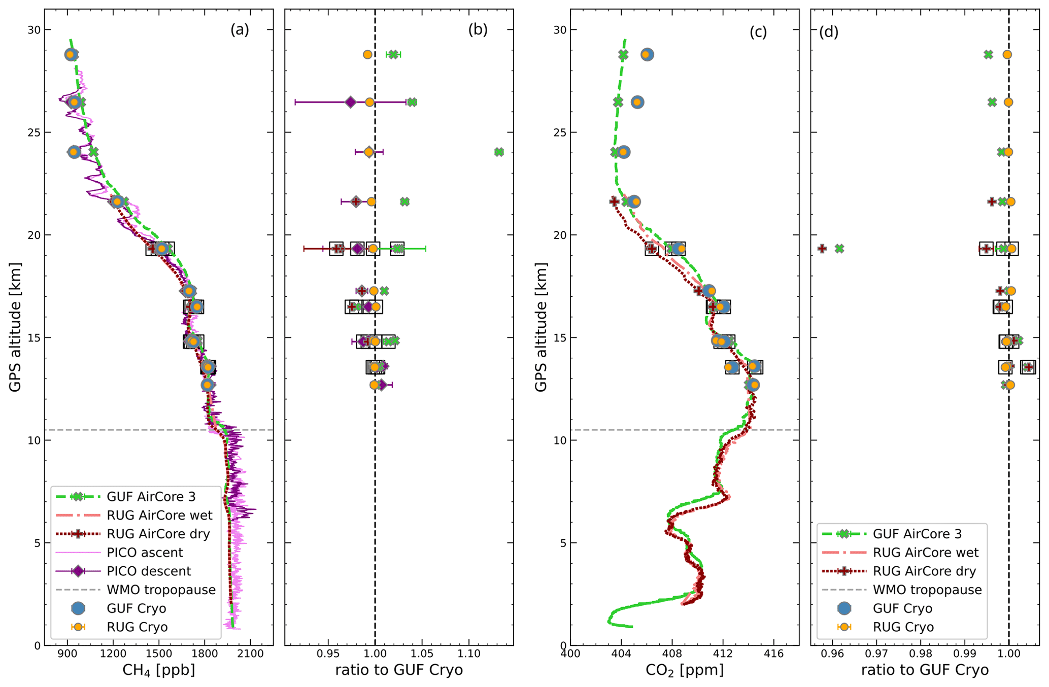
Figure 2 Vertical profiles of CH₄ (a) and CO₂ (c) and comparison with results from the cryosamples as measured at GUF (b, d). To compare results of the high-resolution observations with the samples, the mean value over the sampling period has been calculated using the standard deviation as error bars. Error bars may be smaller than symbol size. Mixing ratios of samples with the cotton scrubber are highlighted by the square symbols.

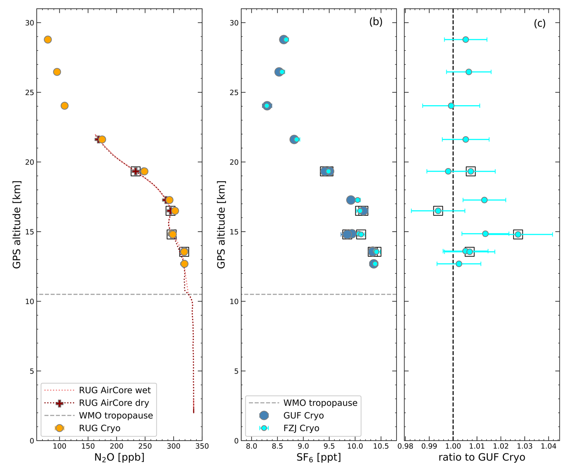
Figure 3 Same as Fig. 2 but for N₂O and SF₆. N₂O was only measured at RUG and no inter-laboratory comparison is possible. Vertical profiles of SF₆ analysed from air samples with GC-ECD (GUF) and GC–MS (FZJ). Error bars of absolute values are smaller than symbol size. For better differentiation, AirCore profiles are plotted as dashed or dotted lines; this does not imply a coarser resolution as profiles are continuous.

In the troposphere, CO₂ mixing ratios show variability between 403 and 413 ppm, and CH₄ mixing ratios vary between 1920 and 1980 ppb in the two AirCore datasets. The high-resolution Pico-SDLA CH₄ data exhibit a tropospheric mixing ratio range from 1920 to 2100 ppb. Above 10 km, CH₄ mixing ratios decrease slowly up to 17 km and decrease steeper with altitude above. Above 20 km, several layers of low CH₄ mixing ratios are apparent in the Pico-SDLA CH₄ data which cannot be resolved by the other measurement methods. CO₂, in contrast, starts to increase at an altitude of approximately 7 km and starts to decrease at around 14 km altitude. A minimum is reached around 24 km altitude. Comparing results from analysis of AirCore and flask samples, N₂O behaves similar to CH₄.

Comparing the two AirCore set-ups (i.e. GUF and RUG), for which data analysis and altitude attribution are done independently, there is an offset of approximately 200–700 m with the RUG AirCore samples being attributed systematically to lower altitudes. The main difference in the processing procedures from GUF and RUG is the fill gas correction. For the RUG AirCore samples, no fill gas correction is performed; therefore, profiles do not extend as high as GUF profiles. An additional uncertainty is introduced for RUG AirCore samples because of the failure of the automatic closing of the inlet after touchdown. This may have caused a loss of sample that could not be corrected. Comparing the two profiles retrieved with and without drying on sampling, the water vapour did not cause a major bias in the retrieved CO₂ and CH₄ molar fractions. In fact, the biggest differences were found in the stratospheric part of the profile, where the atmospheric H₂O content is negligible. In the troposphere, differences between the two AirCore samples at comparable altitudes reached up to 0.4 ppm and 2 ppb for CO₂ and CH₄, respectively. However, the stratospheric part of the profiles showed differences of up to 1.3 ppm for CO₂ and 5 ppb for CH₄. The reasons behind these differences remain overall unclear, but we speculate they could be ascribed to some remaining mixing with the AirCore fill gases or to the interaction of the Mg(ClO₄)₂ dryer with other gas species in the stratosphere.

All flask samples were analysed post-flight at GUF and RUG with the identical instruments that were used for post-flight analyses of AirCore samples. For both laboratories, good agreement within the respective instrumental precisions was found. For CO₂, the average difference is 0.14 ppm, varying between 0.04 and 0.22 ppm. For CH₄, it is 4.3 ppb, varying between 1.8 and 7.4 ppb. Because of the good agreement between the two datasets, measurement results obtained from the cryosampler at GUF are used in the following as a reference for comparison, except for N₂O that was only measured at RUG. Around 14.8 and 13.5 km altitude, overlapping samples with and without a scrubber were collected, although for technical reasons not covering the exact same altitude range, as only one sample flask could be opened or closed at a time. Mixing ratios of CO₂, CH₄, and N₂O agree well for those two sample pairs.

The Pico-SDLA CH₄ is the only instrument of the payload that provides data for the balloon ascent. Although for the lowest altitude part of the profiles the time difference between ascent and descent is almost 7 h, the two measurements agree closely. The spectrometer can resolve small structures in the stratosphere much better than the AirCore samplers which provide a smoothed profile in comparison to Pico-SDLA. When averaging over sample collection times of the cryosampler, which are between 43 and 731 s, very good agreement is found with CH₄ mixing ratios measured post-flight in the laboratories at GUF and RUG. Also, for the sample collected at 24 km altitude, when the spectrometer recorded a local minimum of CH₄ mixing ratios which is not captured by the AirCore observations, both independent post-flight analyses agree. In panels Fig. 2a and c, the variability of the Pico-SDLA CH₄ data is reflected by the larger error bars of the integrated Pico-SDLA CH₄ data, which is most pronounced for the air sample collected at 26.6 km. On average, integrated Pico-SDLA CH₄ data deviate from the sample analysis results in Frankfurt by 9 ppb, with a minimum deviation of 6 ppb and a maximum difference of 25 ppb. In the troposphere, Pico-SDLA CH₄ data are noisier than in the stratosphere, and they are slightly offset towards higher mixing ratios compared to the AirCore profiles. Mixing ratios follow those derived from AirCore measurements but with more fine structures, as the Pico-SDLA CH₄ directly records in situ data, whereas AirCore sampling is a technique with an inherent averaging kernel. Above 20 km, the Pico-SDLA CH₄ profile reveals several layers of lower CH₄ mixing ratios, which cannot be resolved by flask or AirCore samples.

AirCore data have also been averaged over the sampling interval of each cryosampler flask. Differences relative to the direct measurement of CO₂ and CH₄ might partly arise from the uncertainty in altitude attribution. In addition, AirCore samples represent a continuous profile, but due to molecular diffusion some averaging and smoothing with altitude occurs. This becomes most evident when comparing the CH₄ profile derived from AirCore measurements to the in situ recording of CH₄ mixing ratios from the Pico-SDLA CH₄ spectrometer. The Pico-SDLA CH₄ recorded several fine structures above 20 km altitude which are not apparent in the AirCore profiles. Compared to the cryosampler analyses at GUF, GUF AirCore CH₄ integrals tend to be higher by 35 ppb on average, with a minimum difference of 2.2 ppb and a maximum difference of 125.0 ppb, which is observed for the sample collected during a CH₄ minimum of the Pico-SDLA CH₄ profile.

In CO₂, AirCore profiles tend to be at lower mixing ratios in comparison to the cryosampler analyses, particularly at higher altitudes. For data from GUF, the maximum deviation is 1.55 ppm; best agreement is found within 0.14 ppm. Similar results are obtained for the AirCore sample snalyses from RUG for CO₂ and N₂O.

Figure 3b and c compare the results of SF₆ measurements from the air samples in two different laboratories, at GUF and at FZJ. SF₆ is measured with GC-ECD in Frankfurt and with GC–MS in Jülich. Similar to CO₂, SF₆ mixing ratios decrease above the tropopause with the steepest vertical gradient occurring between 17 and 24 km. Results of the two independent measurements agree within their respective uncertainties with a mean difference of 0.04 ppt, varying from 0.01 to 0.27 ppt, corresponding to a relative difference range of 0.08 %–2.7 %. For each instrument, results for the overlapping samples with and without the ozone scrubber agree within the uncertainty. As for CO₂ and CH₄, the steepest gradient in the SF₆ mixing ratios occurs between 17 and 24 km altitude, and, as shown in Fig. 4, there is a clear correlation between SF₆ and the two other greenhouse gases.

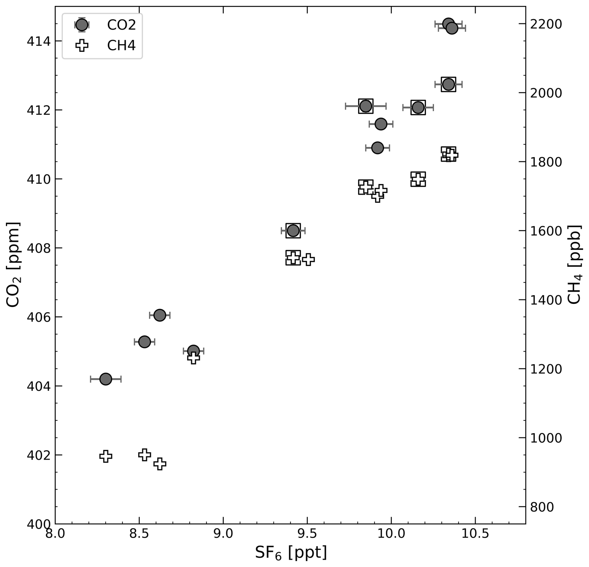
Figure 4 Correlation of CO₂ and CH₄ with SF₆ as analysed from air samples. Mixing ratios of samples with the cotton scrubber are highlighted by the square symbols.

Figure 5 compares age-of-air values derived according to Garny et al. (2024b) from mixing ratios of CO₂ and SF₆ with the tropical marine boundary layer mixing ratios as reference time series (Wagenhäuser et al., 2024). Comparing the results from the flask samples to the AirCore analysis as an example for the GUF AirCore, the systematically higher CO₂ mixing ratios obtained from the flask samples at the highest altitudes are reflected as lower age-of-air vales. However, the general structure of the profiles agree, particularly at altitudes below 20 km. This confirms that AirCore is a measurement technique suited to derive age-of-air profiles from CO₂ observations.

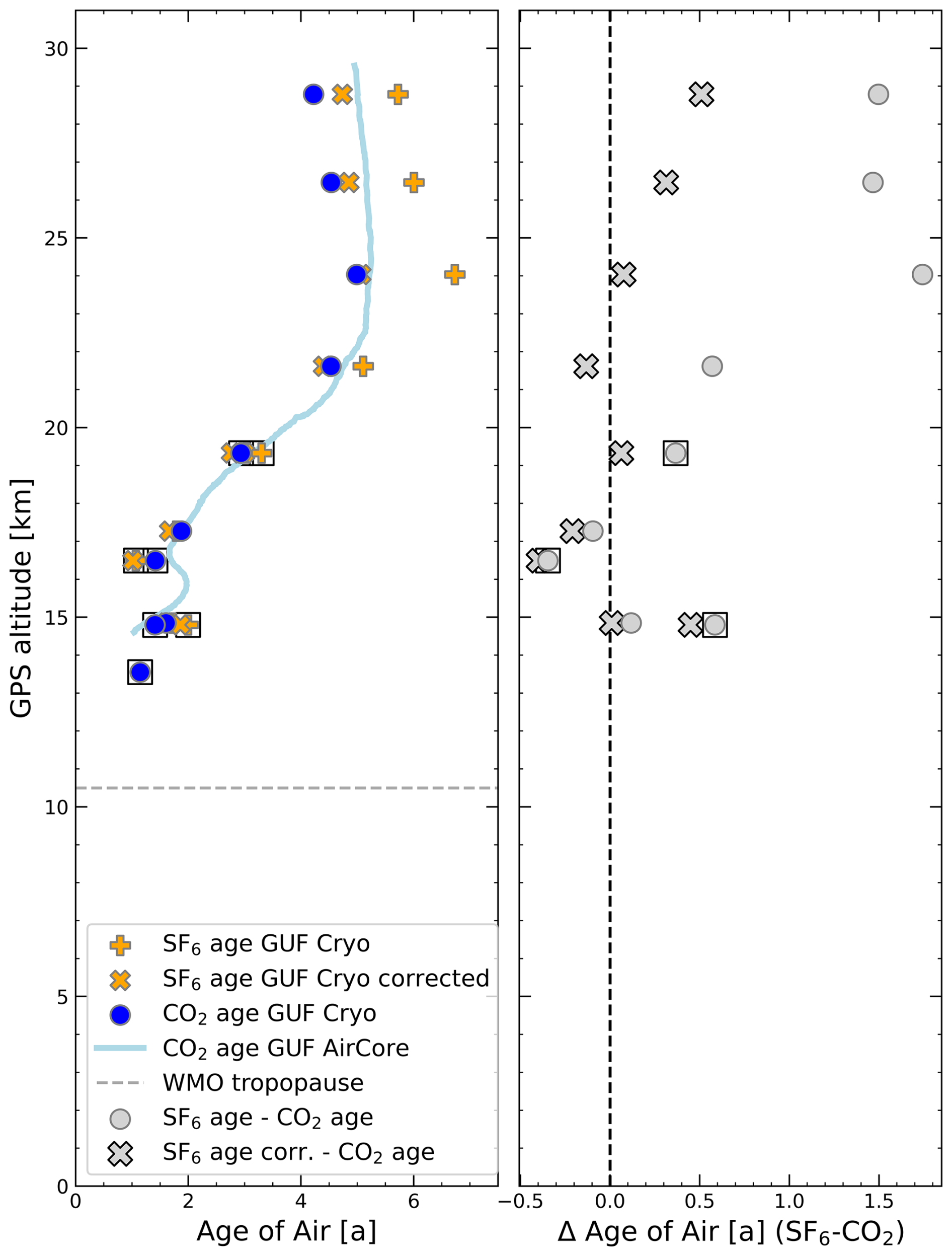
Figure 5 Age-of-air values derived from CO₂ and SF₆ mixing ratios of flask air samples and AirCore CO₂ mixing ratios. Samples with the cotton scrubber are highlighted by the square symbols. “×” markers represent age-of-air values from SF₆ mixing ratios corrected using the method by Garny et al. (2024a).

For CO₂, systematically lower ages are derived, with the difference increasing with altitude. This agrees with findings by Ray et al. (2024), who consistently analysed a large number of dataset from aircraft and balloon-borne measurements for the periods 1994–2000 and 2021–2024, including AirCore data for the latter period. In the 2021 HEMERA TWIN dataset, the difference increases to 1.5 years at altitudes around 24 km and above. Using the bias correction described by Garny et al. (2024a) to account for chemical sinks of SF₆ reduces the SF₆ age by 0.05–1.67 years with an average reduction of 0.55 years. The corrected values range from 1–5 years with maximum ages of 4.4–5.1 years above 20 km altitude. The corrected SF₆ agrees better with the value derived from CO₂ with the average difference reducing from 0.66 to 0.08 years when applying the correction.

4 Conclusions

Within the HEMERA balloon infrastructure project coordinated by the French space agency CNES, the openly constructed TWIN gondola was launched from Kiruna, Sweden, in August 2021. The gondola was equipped with two different air samplers, three different types of AirCore set-ups, and the mid-infrared diode laser spectrometer Pico-SDLA CH₄ for in situ measurements of CH₄. A maximum altitude of 31.2 km was reached. Here, we reported on analysis results for CO₂, CH₄, and SF₆ from cryogenically collected air samples in stainless-steel flasks. Samples were analysed post-flight in different laboratories using optical and gas chromatography measurement techniques. Mixing ratios of all three greenhouse gases agree well for the different analyses.

Results are compared to vertical profiles of CO₂ and CH₄ derived from AirCore samples and to CH₄ measured with the Pico-SDLA. The latter instrument records more fine structures at altitudes above 20 km, which is not apparent in the AirCore data with much smoother profiles. While the agreement between the Pico-SDLA CH₄ measurements and the air sample analysis is very good for CH₄, AirCore-derived CH₄ measurements deviate, likely because the AirCore cannot resolve the observed minima in the CH₄ profile. Additional uncertainty arises from the altitude attribution of the AirCore profiles. This becomes more apparent in the case of CO₂, for which the difference between air sample analyses and AirCore profiles seems to increase with altitude. In addition, differences between two independent AirCore datasets are observed, with altitude differences of individual features of up to 300 m.

For CO₂ and SF₆, age of air was derived from the observations following the approach by Garny et al. (2024b). At altitudes of 24 km and above, maximum ages between 5.8 and 6.5 years were obtained from SF₆ mixing ratios, which reduced to 4.4–5.1 years after correction of the chemical sink according to Garny et al. (2024a). Age-of-air values derived from CO₂ are systematically lower, with the difference increasing with altitude, in agreement with the finding from other datasets. Up to an altitude of 25 km, age of air derived from AirCore analysis of CO₂ agrees well with flask sample data; at higher altitudes, differences occur. Accounting for chemical sinks of SF₆, the SF₆-based age of air decreases and better agrees with CO₂-derived age of air within 0.5 years. Recently, Ray et al. (2024) proposed a new technique of deriving age of air from simultaneous measurements of several long-lived trace gases. The dataset presented here, containing CO₂, CH₄, and SF₆, should be well suited for this approach. The dataset, which will be complemented by further data of halogenated long-lived trace gases (Laube et al., 2025), will enable further age-of-air evaluations.