Technical note: Water vapour climatologies in the extra-tropical upper troposphere and lower stratosphere derived from a synthesis of passenger and research aircraft measurements

This study presents a new methodology to derive adjusted water vapour (H₂O) climatologies for the extra-tropical upper troposphere and lowermost stratosphere (UT/LMS) from regular measurements on board passenger aircraft between 1994 and 2022 within the IAGOS (In-service Aircraft for a Global Observing System) research infrastructure. A synthesis of mean H₂O is performed by sampling air mass bins of similar origin and thermodynamic conditions relative to the tropopause between a dataset from 60 000 flights employing the IAGOS-MOZAIC (Measurement of Ozone by AIRBUS In-Service Aircraft) and IAGOS-CORE capacitive hygrometer (ICH) and a dataset of 500 flights using the more sophisticated IAGOS-CARIBIC (Civil Aircraft for the Regular Investigation of the Atmosphere Based on an Instrument Container) hygrometer. The analysis is, in combination with ECMWF ERA5 meteorological data, accomplished for the extra-tropical Northern Hemisphere, where the datasets have the largest common coverage. We find very good agreement in the UT but a systematic positive humidity bias in the ICH measurements for the LMS. To account for this bias, mean H₂O of the ICH is adjusted to the IAGOS-CARIBIC measurements based on a new mapping and adjustment approach. After applying this new method, the LMS H₂O measurements are in good agreement between all investigated platforms. The extensive H₂O dataset from the compact IAGOS sensor can now be used to produce highly resolved H₂O climatologies for the climatically sensitive LMS region.

1 Introduction

Over the past decades, upper troposphere and lowermost stratosphere (UT/LMS) water vapour (H₂O) has gained increasing attention due to its significant impact on the global climate system (IPCC, 2023). Apart from the influence on ozone concentration (Kirk-Davidoff et al., 1999) and cirrus cloud formation, even small variations in UT/LMS H₂O lead to substantial changes in radiative forcing (Riese et al., 2012; Banerjee et al., 2019; Gettelman et al., 2011). Radiative forcing calculations suggest that the increase in stratospheric H₂O of 0.8 ppmv as derived from balloon soundings between 1980–2000 could have accounted for 30 % of the total anthropogenic forcing during that time period (Forster and Shine, 2002). On the other hand, satellite-borne measurements going back to the 1980s have not shown significant long-term trends in stratospheric H₂O over several decades (Hegglin et al., 2014; Konopka et al., 2022). For the future, however, most global climate models predict an increase in stratospheric H₂O (e.g. Banerjee et al., 2019; Huang et al., 2020) and a corresponding total stratospheric water vapour radiative feedback parameter of 0.2–0.3 W m⁻² per 1 K of surface warming (Forster and Shine, 2002; Huang et al., 2020; Nowack et al., 2023). Nevertheless, there are still significant uncertainties in predicting the radiative forcing resulting from changes in stratospheric H₂O (Huang et al., 2020). One of the reasons is that the low stratospheric H₂O concentrations below 10 ppmv and the even smaller changes are difficult to detect with required statistical significance. Therefore, the accurate detection of UT/LMS H₂O, as well as trends at high temporal and spatial resolution, is essential to better understand the role of H₂O in this part of the atmosphere for the global climate system.

Global observation of H₂O in the UT/LMS is provided by space-borne remote sensing instruments, such as the Microwave Limb Sounder (Hegglin et al., 2013). Due to their limited vertical resolution of several kilometres, however, the space-borne observations cannot adequately resolve the high vertical gradients of H₂O across the extra-tropical tropopause layer (Gettelman et al., 2011; Zahn et al., 2014). To address this limitation and provide UT/LMS H₂O profiles with a high vertical resolution, airborne in situ measurements play a crucial role. The IAGOS (In-service Aircraft for a Global Observing System; http://www.iagos.org, last access: 7 April 2025) database offers H₂O measurements from over 60 000 passenger aircraft flights, enabling the resolution of the strong vertical and temporal H₂O variations in the UT/LMS of the extra-tropical Northern Hemisphere (Zahn et al., 2014; Petzold et al., 2020). For instance, based on IAGOS observations over North America, the North Atlantic and Europe (40–60° N each), Petzold et al. (2020) were able to resolve the pronounced seasonality of UT/LMS H₂O in these regions with a vertical resolution of 0.3 km. This study revealed a near doubling of the H₂O mixing ratio during summer compared to winter in the UT and the first kilometre above the thermal tropopause, with the strongest seasonality observed over the North Atlantic. The investigation of these seasonal and spatial UT/LMS H₂O variations based on IAGOS measurements helps to quantify and understand the processes that control the temporal and spatial variability in H₂O. These can be seasonal variations attributed to the Brewer–Dobson circulation and isentropic transport or short-term micro- to mesoscale H₂O mixing between troposphere and stratosphere associated with turbulence and diabatic processes like overshooting convection (Gettelman et al., 2011). A better understanding of these processes helps to improve their representation in climate models. In this context, the large quantity of in situ H₂O measurements provided by IAGOS is important for improving the accuracy of future H₂O and corresponding radiative forcing trends based on climate model predictions.

The IAGOS database consists of three datasets with instrument packages of different kinds: IAGOS-MOZAIC (MOZAIC: Measurement of Ozone by AIRBUS In-Service Aircraft; Marenco et al., 1998), IAGOS-CORE (Petzold et al., 2015) and IAGOS-CARIBIC (Civil Aircraft for the Regular Investigation of the Atmosphere Based on an Instrument Container; Dyroff et al., 2015). The MOZAIC project was the predecessor programme to IAGOS-CORE, and the data were integrated into the IAGOS database afterwards. Combined, IAGOS-MOZAIC and IAGOS-CORE contain ∼60 000 flights, both providing humidity measurements with a compact capacitive humidity sensor of the same type (ICH; Neis et al., 2015a). Compared to IAGOS-MOZAIC and IAGOS-CORE, the IAGOS-CARIBIC dataset consists of a relatively small number of flights of $\sim \mathrm{500}.$ The IAGOS-CARIBIC package consists of sophisticated instruments, enabling high-precision measurements of H₂O even for very low stratospheric concentrations (Zahn et al., 2014). The ICH measurements, however, were found to lose precision for very dry stratospheric air masses (Kunz et al., 2008; Rolf et al., 2023). In a previous intercomparison of IAGOS H₂O observations (at that time taken in the framework of the MOZAIC project) and research-aircraft-based observations as part of the SPURT (Spurenstofftransport in der Tropopausenregion, trace gas transport in the tropopause region; Engel et al., 2006) project, a lower H₂O threshold for precise measurements of 10 ppmv was determined for the ICH at conditions typical of the extra-tropical LMS (Kunz et al., 2008). This lower detection limit for the ICH instrument was later determined to be 30 ppmv by means of a dedicated hygrometer intercomparison study (Rolf et al., 2023).

The aim of this study is to provide an improved dataset by mapping and adjusting the IAGOS-MOZAIC and IAGOS-CORE measurements to observations from more precise instruments. Therefore, in order to quantify the H₂O bias of IAGOS-MOZAIC and IAGOS-CORE in the LMS, the first step of this study is to compare these data with the IAGOS-CARIBIC measurements that are able to resolve low LMS H₂O. Furthermore, sophisticated campaign measurements from 500 flights summarised in the JULIA (Jülich In-situ Airborne Data Base; Krämer et al., 2020) database are included in the comparison.

The main challenge is to devise an approach that allows for a valid intercomparison of the in situ H₂O datasets despite the limited amount of IAGOS-CARIBIC and JULIA data and the fact that the measurements of the datasets were performed on different platforms at different times and in different regions. To address this challenge, we apply a robust new mapping methodology that enables an accurate comparison of H₂O in air masses of similar atmospheric origin, thermodynamic conditions and seasons. Through this comparison, we can identify and quantify biases in the H₂O measurements by IAGOS-MOZAIC and IAGOS-CORE in the LMS.

Based on the results of this intercomparison, we develop an adjustment methodology to the IAGOS-MOZAIC and IAGOS-CORE H₂O datasets in the LMS. This methodology allows us to account for the biases identified in the intercomparison, ensuring improved accuracy in the representation of the H₂O variability in the UT/LMS at northern mid-latitudes.

The paper is structured as follows: in Sect. 2, we provide a comprehensive overview of the datasets that are utilised in the comparison presented in Sect. 3. Section 4 outlines the methodology employed for mapping and adjusting the IAGOS-MOZAIC and IAGOS-CORE LMS H₂O climatologies in dry LMS regions. In Sect. 5, we summarise the key findings and provide an outlook on potential future research based on the adjusted IAGOS-MOZAIC and IAGOS-CORE H₂O climatologies.

2 H₂O datasets

2.1 Airborne in situ H₂O measurements

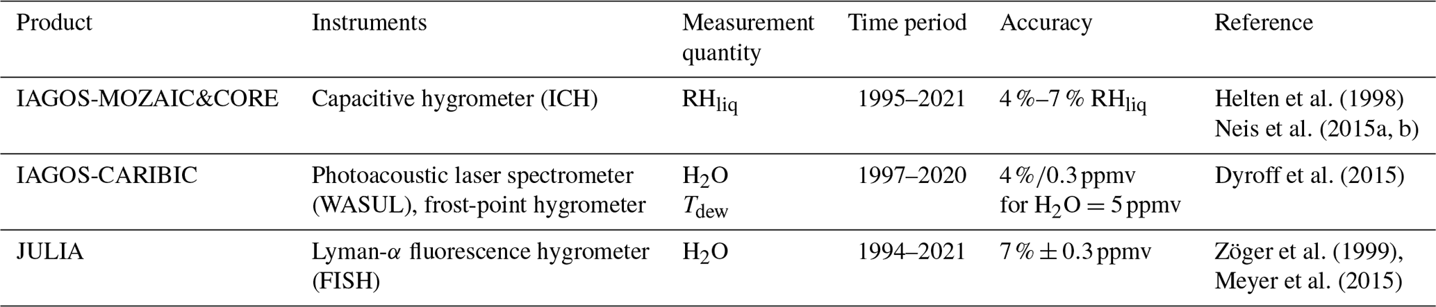
Two sets of IAGOS H₂O data from about 3 decades of airborne in situ measurements with a compact capacitive hygrometer (IAGOS capacitive hygrometer: ICH; see Sect. 2.1.1), IAGOS-MOZAIC and IAGOS-CORE, are the basis of this study and are combined into one dataset (IAGOS-MOZAIC&CORE). This extensive dataset is validated against two others, IAGOS-CARIBIC and JULIA, which are smaller but have measured H₂O with more accurate instruments. The IAGOS-CARIBIC water instrument applies two different sensor systems (WaSul – photoacoustic laser spectrometer – and frost-point hygrometer; see Sect. 2.1.2). The JULIA database primarily contains data from the high-precision hygrometer FISH (Fast In-situ Stratospheric Hygrometer; Sect. 2.1.3). The datasets are summarised in Table 1. A detailed intercomparison study of ICH, WaSul and FISH on board a Learjet research aircraft was conducted as part of the DENCHAR project (Rolf et al., 2023).

Helten et al. (1998)Dyroff et al. (2015)Zöger et al. (1999)Meyer et al. (2015)

Table 1 Summary of the UT and LS airborne in situ H₂O datasets.

2.1.1 H₂O dataset from passenger aircraft: IAGOS-MOZAIC&CORE

The IAGOS-MOZAIC&CORE dataset (from now on just MOZAIC&CORE) (https://www.iagos.org/, last access: 7 April 2025) provides measurements of the relative humidity with respect to liquid (RH_liq) taken by the compact capacitive sensor ICH on board commercial aircraft in the period from 1995 to this day and derived H₂O mixing ratios. The ICH relies on a water-adsorbing dielectric membrane between two parallel electrodes with its dielectric capacity depending on the relative humidity of the surrounding air. Measurements are provided every 4 s, which corresponds to a horizontal resolution of about 1 km. The instruments are removed from the aircraft every 3 months and are calibrated against a reference frost-point hygrometer in an atmospheric simulation chamber before being re-installed again. Details of the current instrument handling and data processing are described by Petzold et al. (2020).

The largest number of the 60 000 flights in the dataset took place in the northern mid-latitudes between Europe and North America (Fig. 1a). Here, at flight altitudes of 9–13 km, heights of up to 5 km above the tropopause can be reached, especially during the winter season on northern routes, while in the tropics only the upper troposphere is covered (Fig. 1d).

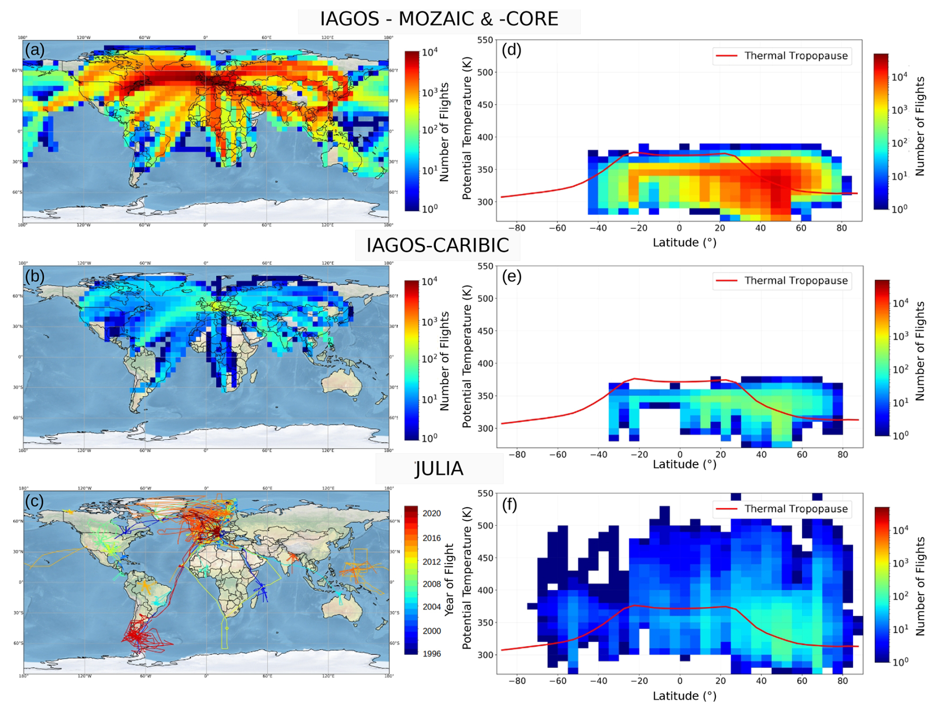
Figure 1 Geographical distribution of H₂O measurements. The plots indicate the flight density of IAGOS-MOZAIC&CORE, IAGOS-CARIBIC and JULIA both horizontally (a–c) and vertically (d–f). In (a)–(c), the flight density is given on a 5°×5° grid for the IAGOS datasets, while for JULIA the single flight tracks and corresponding years are shown. Potential temperature is taken as the vertical coordinate (d–f) with a resolution of 5 K and a latitude resolution of 5°; the solid red lines represent the average thermal tropopause, calculated from ERA5 data.

2.1.2 H₂O dataset from passenger aircraft: IAGOS-CARIBIC

The IAGOS-CARIBIC dataset (from now on just CARIBIC) provides measurements from more than 500 long-distance passenger aircraft flights (Fig. 1b and e) in the period from 1997 to 2020. The instruments installed in the CARIBIC Flying Laboratory measure about 100 tracers and aerosol parameters (https://www.CARIBIC-atmospheric.com, last access: 7 April 2025), including water vapour and total (gaseous-, liquid- and ice-phase) water.

Compared to MOZAIC&CORE, measurements are taken by more advanced instrumentation. The CARIBIC water instrument applies two different sensor systems (measurement techniques): a modified (dual-channel photo-acoustic laser spectrometer) WaSul sensor (for total and gas-phase water) and a modified CR2 Buck frost-point hygrometer (FPH) sensor, with the FPH being used for a regular in-flight calibration of the WaSul sensor (Dyroff et al., 2015).

2.1.3 H₂O dataset from research aircraft: JULIA

The Jülich In-situ Airborne Data Base (JULIA) contains H₂O data from more than 500 research aircraft flights during 46 campaigns that took place from 1994 onward. It contains precise measurements from advanced instrumentation of trace gases, like H₂O, and cloud microphysical properties (Krämer et al., 2020). H₂O data are provided by instruments that have a high sensitivity to low stratospheric H₂O, with most measurements being performed by the Fast In-situ Stratospheric Hygrometer (FISH; Zöger et al., 1999), which is sensitive to low UT/LMS H₂O, with an accuracy of 6 %–8 % between 1 and 1000 ppmv (Meyer et al., 2015). In contrast to the IAGOS flights, the research aircraft flights often reach deeper into the stratosphere and also cover the tropical lower stratosphere (LS), with altitudes of up to 20 km, which corresponds to potential temperatures of more than 500 K (Fig. 1).

2.2 ECMWF ERA5 reanalysis data

The ERA5 reanalysis data (Hersbach et al., 2020) from the European Centre for Medium-Range Weather Forecasts (ECMWF) provide meteorological parameters every hour in the period from 1959 onward. The ERA5 data are given on a 30 km horizontal resolution with 137 vertical model levels, reaching heights of up to 0.1 hPa. For this study, ERA5 data are used at a reduced resolution of 6 h and 1°×1° but with the original vertical resolution. Along the flight paths of passenger (IAGOS) and research (JULIA) aircraft, the position relative to the first and, if present, second WMO thermal tropopause as well as the equivalent latitude derived from the potential vorticity fields is interpolated.

3 Intercomparison of airborne in situ H₂O datasets

In this section, a comparative analysis of the in situ H₂O products is performed, focusing on the UT/LMS region. Given the similar performance found in this study for the MOZAIC and CORE measurements, as detailed in Sect. 3.3, the primary emphasis is on the MOZAIC data, with the findings also accounting for CORE.

Figure 2a–c presents latitudinal cross-sections of H₂O for the winter (December–February) season, using a resolution of 5° latitude × 5 K potential temperature based on all available data from the different datasets. In the mid- to high latitudes, potential temperature levels above 350 K predominantly correspond to air masses in the LMS during the winter season. Here, the mean H₂O values of MOZAIC are significantly higher (10–20 ppmv) than the values reported by CARIBIC and JULIA (5–10 ppmv).

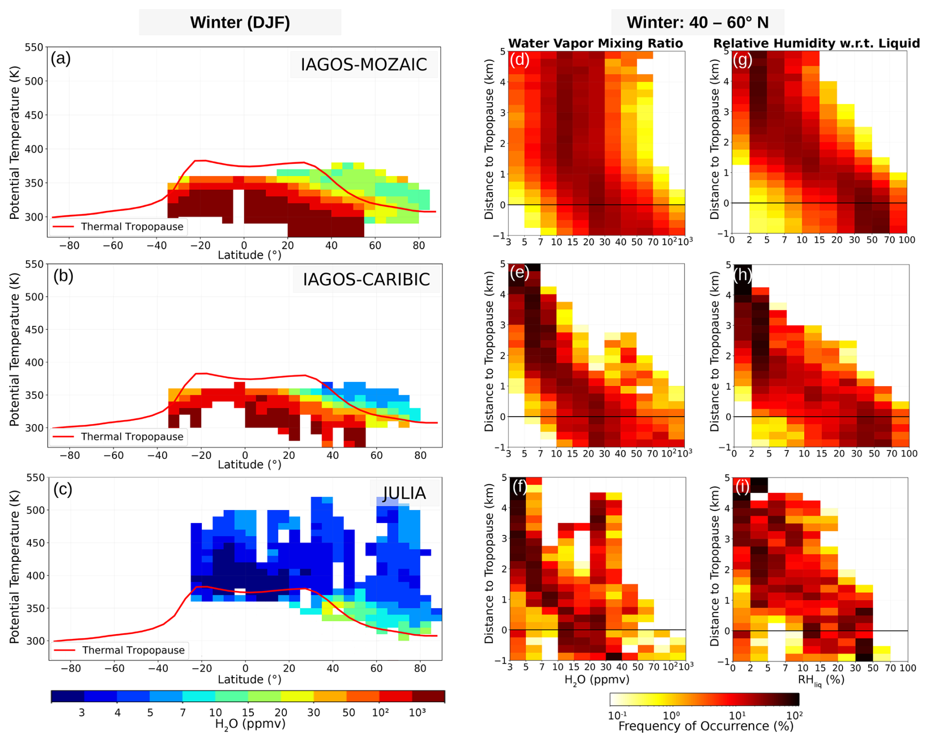
Figure 2 Multi-annual latitudinal cross sections of H₂O for the datasets IAGOS-MOZAIC&CORE, IAGOS-CARIBIC and JULIA. Panels (a–c) show the winter (December–February) mean H₂O binned in 5° latitude × 5 K potential temperature bins; the solid red lines represent the average thermal tropopause, calculated from ERA5 data. For the winter season at 40–60° N, the probability density in coordinates relative to the thermal tropopause (Δz) and normalised per Δz is shown for H₂O (d–f) and RH_liq (g–i).

The H₂O frequency distribution relative to the thermal tropopause (TTP; altitude bin width: 0.25 km) shown in Fig. 2d–f for the winter 40–60° N domain underpins the noticeable contrasts between the three datasets. Specifically for MOZAIC, a consistent moist bias is evident from heights of 1 km above the TTP. This bias is becoming more pronounced at higher altitudes. Additionally, MOZAIC shows a more pronounced H₂O variability compared to CARIBIC and JULIA at heights of 1 km above the TTP. This behaviour is closely linked to the magnitude of RH_liq measured by the ICH sensor. The RH_liq data from CARIBIC and JULIA indicate that RH_liq values frequently drop below 10 % at these altitudes, and they are often below 5 % at altitudes of 3 km and higher than the TTP (Fig. 2h and i). In contrast, the RH_liq profile of MOZAIC displays a less strong decrease in RH_liq in the LMS and generally higher values compared to CARIBIC and JULIA.

The reason for this loss of sensitivity of the ICH sensor in the LMS is attributed to the adiabatic compression effect. As the air flows into the inlet towards the sensor, it undergoes heating in the range of 20–30 K. Consequently, even though the stratospheric humidity values are already very low, the measured values at the sensor decrease by a factor of 10, resulting in a sensitivity loss of the ICH for these very low relative humidity values below ≈10 % RH_liq (Neis et al., 2015a, b). More details about this effect are discussed in Petzold et al. (2020). Despite the systematic biases at low RH_liq, the ICH sensor demonstrates a measurable response beyond the noise level, even at RH_liq values as low as approximately 1 % (Neis et al., 2015a; Rolf et al., 2023).

When comparing the H₂O distributions shown in Fig. 2e and f between JULIA and CARIBIC, both originating from sensors sensitive to low stratospheric H₂O values, still some differences are noticeable. First, the spatial and seasonal coverage of JULIA and CARIBIC datasets differs, contrary to the very good temporal and spatial agreement between CARIBIC and MOZAIC&CORE (Fig. 1). Moreover, the research campaign measurements in JULIA were often conducted under specific atmospheric conditions, such as during troposphere-to-stratosphere exchange events. As a result, cases of anomalous H₂O concentrations may be over-represented in the JULIA dataset. This is evident, for instance, in a frequency of occurrence of H₂O between 20 and 50 ppmv at distances of 3 km and more above the thermal tropopause (TTP) in Fig. 2f, where the mean winter extra-tropical H₂O values are expected to be below 10 ppmv on average (Zahn et al., 2014). However, at higher altitudes, corresponding to potential temperatures above 400 K, JULIA provides a climatological perspective of H₂O from the tropics to the northern sub-polar regions (Fig. 2c). In these potential temperature ranges, H₂O concentrations exhibit seasonal variations due to the Brewer–Dobson circulation, while the effects of short-term UT-to-LMS mixing processes do not significantly contribute to the H₂O distribution on a short timescale on the order of days (Gettelman et al., 2011).

As discussed in this section, MOZAIC&CORE overestimate H₂O in most parts of the extra-tropical LMS due to sensor limitations in capturing low values of RH_liq values that are common in this part of the atmosphere. To further quantify the MOZAIC&CORE bias in the LMS, we developed an air mass mapping approach that allows for a better intercomparison with the CARIBIC H₂O data. This method will be detailed in the next section.

3.1 Mapping approach to compare in situ H₂O datasets

A mapping approach is used as the method of evaluation of MOZAIC&CORE on the basis of CARIBIC, focusing on the primary variable measured by MOZAIC&CORE, RH_liq. The main challenge in this intercomparison is to ensure data comparability given the relatively small amount of CARIBIC data (500 flights) compared to the large amount of MOZAIC&CORE data (together 60 000 flights). The relatively small number of CARIBIC data points could introduce non-negligible uncertainties in the statistical comparison due to the natural variability in UT/LMS H₂O caused by competing transport, chemical and mixing processes near the tropopause. These factors particularly affect the UT and the extra-tropical transition layer (exTL) (Zahn et al., 2014), whereas H₂O above the exTL exhibits much smaller variations (Gettelman et al., 2011). To minimise this uncertainty, a careful temporal and spatial sampling is performed using a geophysically based coordinate system known to reduce sampling biases (Millan et al., 2023). The methodology is summarised in Fig. 3.

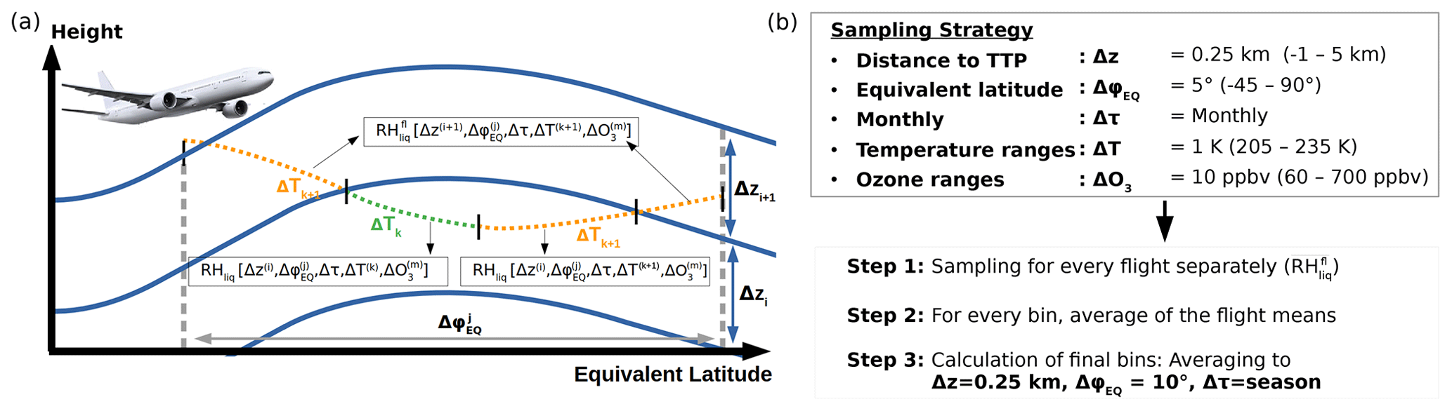
Figure 3 Schematic illustration of the data sampling strategy to compare the different H₂O products. (a) The blue lines indicate constant height levels relative to the tropopause, and the two dashed grey lines mark a 5° equivalent latitude bin. The dotted line illustrates the flight path, with the different colours indicating different temperature ranges. See top box of (b) for the definition of the sampling bins of distance to the thermal tropopause (Δz), equivalent latitude (Δφ_EQ), time (Δτ), temperature (ΔT) and ozone (ΔO₃). The bottom box of (b) lists the different steps to derive the final sampling bins used for the intercomparison of the H₂O datasets.

Spatially, the H₂O data are sampled relative to the TTP (Δz_TTP) obtained from ERA5. The sampling starts 1 km below the TTP with a vertical resolution of 0.25 km and is done in equivalent latitude ranges (Δφ_EQ) of 5°. Cases with double tropopauses were excluded from the analysis. We found that incorporating the dynamical tropopause, defined as 2 potential vorticity units (PVU; 1 PVU $={\mathrm{10}}^{-\mathrm{6}}\mathrm{K}{\mathrm{m}}^{\mathrm{2}}{\mathrm{s}}^{-\mathrm{1}}{\mathrm{kg}}^{-\mathrm{1}}$) neither improved nor worsened the quality of the resulting intercomparison. Instead of using latitudinal mean values of H₂O, means corresponding to ERA5-equivalent latitude are calculated because the potential-vorticity-based equivalent latitude characterises the latitudinal air mass origin in the upper troposphere and lower stratosphere (Gettelman et al., 2011), as well as the corresponding H₂O mixing ratios to some extent.

On a temporal scale, we calculate monthly means (Δτ_month) to account for the seasonal variability in UT/LMS H₂O (Zahn et al., 2014; Petzold et al., 2020). Since H₂O data of MOZAIC&CORE are derived from RH_liq measurements, which depend on temperature, we further divide each bin ($\mathrm{\Delta }{z}_{\text{TTP}},\mathrm{\Delta }{\mathit{\phi }}_{\text{EQ}},\mathrm{\Delta }{\mathit{\tau }}_{\text{month}}$) into temperature ranges (ΔT) of 1 K. This temperature sampling ensures that any potential discrepancies in the sampled RH_liq due to differences in the temperature distribution between MOZAIC&CORE and CARIBIC are accounted for. Additionally, the temperature at a certain height level can correlate with atmospheric conditions, which in turn can influence the H₂O values. Although we also performed a potential temperature sampling, it did not yield significant differences in the final intercomparisons and was therefore not used in the final sampling strategy. The temperature sub-sampling at specific heights essentially achieves the same effect as the potential temperature sampling given the relatively stable flight pressure levels.

To enhance the statistical comparability, we incorporate ozone measurements that were conducted during the majority of MOZAIC&CORE and CARIBIC flights. Bethan et al. (1996) and Sprung and Zahn (2010) demonstrated that ozone measurements are effective in delineating the structure of the LMS. Above the tropopause, the characteristic increase in ozone concentrations makes it a suitable stratospheric tracer and can be indicative of stratospheric air masses to resolve UT/LMS mixing processes. Therefore, for each bin sampled above the thermal tropopause, we further sub-sample the air masses based on ozone concentrations in steps of ΔO₃=10 ppbv, spanning the range from 60 to 700 ppbv.

The binning process ($\mathrm{\Delta }{z}_{\text{TTP}},\mathrm{\Delta }{\mathit{\phi }}_{\text{EQ}},\mathrm{\Delta }{\mathit{\tau }}_{\text{month}},\mathrm{\Delta }T,\mathrm{\Delta }{\mathrm{O}}_{\mathrm{3}}$) is conducted for each flight individually (Fig. 3a and b – Step 1). For every measurement that falls into a respective sampling bin and flight, we compute the sampling means $\stackrel{\mathrm{‾}}{\text{RH}{}_{\text{liq}}^{\text{fl}}}$ (see Fig. 3a). To derive a relevant sampling mean, a minimum of 10 data points are required per bin and flight. Subsequently, for each of these bins, the arithmetic mean is computed from all the mean values obtained from the individual flights:

$$\begin{array}{}\text{(1)}& {\displaystyle }{\displaystyle }\stackrel{\mathrm{‾}}{\text{RH}{}_{\text{liq}}^{*}}={\displaystyle \frac{\mathrm{1}}{N_{\text{fl}}^{*}}}\sum _{i=\mathrm{0}}^{N_{\text{fl}}}\stackrel{\mathrm{‾}}{\text{RH}{}_{\text{liq}}^{\text{fl}}\left[i\right]},\end{array}$$

where $N_{\text{fl}}^{*}$ is the total number of flights for a certain sampling bin.

Data from different flights are weighted equally to mitigate the potential influence of measurements from individual flights that might have a larger number of observations compared to most other flights. This equal weighting is particularly crucial for the sampling of CARIBIC data, where some bins may contain data from 10 flights or fewer, making it necessary to ensure appropriate representation of all flights in the analysis.

In the final step, to ensure a sufficient number of bins with enough data to serve as a valid reference, we derive weighted seasonal averages (DJF, MAM, JJA, SON) from the monthly means and 10° weighted Δφ_EQ means from the 5° Δφ_EQ means. Additionally, we calculate the weighted mean across all 1 K ΔT and 10 ppbv ΔO₃ ranges. In this averaging process, each bin is weighted based on the number of CARIBIC flights ($N_{\text{fl}}^{{\text{CA}}^{*}}$) that contribute to the mean values (see Eq. 1) in every 1 K ΔT, 10 ppbv ΔO₃, 5° Δφ_EQ, and monthly range:

$$\begin{array}{ll}{\displaystyle }& {\displaystyle }\stackrel{\mathrm{‾}}{\text{RH}{}_{\text{liq}}}={\displaystyle \frac{\mathrm{1}}{N_{\text{fl}}^{\text{CA}}}}\sum _{i=\mathrm{0}}^n\stackrel{\mathrm{‾}}{\text{RH}{}_{\text{liq}}^{*}}\left[i\right]\times N_{\text{fl}}^{\text{CA}}\left[i\right],\\ \text{(2)}& {\displaystyle }& {\displaystyle }\text{with}{N}_{\text{fl}}^{\text{CA}}=\sum _{i=\mathrm{0}}^n{N_{\text{fl}}^{\text{CA}}}^{*}\left[i\right],\end{array}$$

where n is the number of bins that contribute to $\stackrel{\mathrm{‾}}{\text{RH}{}_{\text{liq}}}$.

This weighted-averaging approach ensures that each bin is appropriately represented in the final intercomparison, taking into account the relatively small number of flights available in the CARIBIC dataset compared to MOZAIC&CORE. For instance, in the calculation of seasonal means from the respective monthly means, a higher number of flights during a particular month by CARIBIC compared to MOZAIC&CORE could lead to an over-representation of that month in the CARIBIC seasonal mean, affecting the overall intercomparison results. Since H₂O in the extra-tropical UT/LMS exhibits non-negligible variations on a monthly scale (Zahn et al., 2014; Kunz et al., 2008), this weighting is crucial to ensure an appropriate comparison between the datasets and to obtain reliable and meaningful results. Overall, this approach was found to significantly improve the accuracy of the statistical comparability of the datasets.

By applying the mapping approach described above, sampling bins that contain too few flights are excluded, as these could lead to higher uncertainties due to the natural variability in H₂O in the UT/LMS despite the use of the geophysically based coordinate system. This uncertainty is expected to decrease with height above the tropopause, as has been shown for H₂O based on the calculation of a trade-off factor between including more measurements vs. adding more geophysical variability (due to year-to-year or longitudinal variations). This trade-off factor shows that fewer measurements are needed to constrain the mean H₂O value in a certain bin the higher above the tropopause it lies (Hegglin et al., 2008), providing confidence in our approach. Thus, the minimum number of flights required for a sampling bin to be included in the final intercomparison varies with the height relative to the TTP. Specifically, the minimum number of flights linearly decreases from 15 in the lowest vertical range below the TTP (−1 to −0.75 km) to 4 flights at 3 km and higher above the TTP.

Despite the relatively limited number of flights available in the CARIBIC dataset, a considerable number of sampling bins (Δz_TTP=0.25 km, Δφ_EQ=10°, Δτ_season) contain a sufficient number of data and flights through the years to represent the multi-annual climatological state and thus enable a reliable intercomparison with MOZAIC&CORE (as detailed in Sect. 3.3).

3.2 Intercomparison of IAGOS-CARIBIC and JULIA H₂O

H₂O data from CARIBIC serve as a reference for evaluating the extensive dataset of MOZAIC&CORE. To ensure the high quality of the CARIBIC data, the performance of the CARIBIC H₂O measurements (combination of WaSul and FPH; see Sect. 2.1.2 and Zahn et al., 2014) is validated by a comparison with high-precision instruments, such as FISH, compiled in the research aircraft dataset JULIA (Sect. 2.1.3). In the past, joint flights of the WaSul sensor and the FISH hygrometer were conducted, enabling a direct comparison of H₂O measurements from both instruments (Meyer et al., 2015; Tatrai et al., 2015; Rolf et al., 2023). While notable differences outside the expected noise level were observed between the two instruments in dry stratospheric air masses of 10 ppmv and less, no systematic bias in either the dry or wet direction was identified (Tatrai et al., 2015).

3.2.1 Preparation of the datasets

For the comparison of CARIBIC and JULIA H₂O data in the LMS, the binning strategy described in Sect. 3.1 and depicted in Fig. 3 is employed. In the comparison, only sampling bins at distances of at least 1.5 km above the TTP are included. This reduces the impact of the natural H₂O variability on the comparison, which is higher close to the TTP and in the UT.

The higher sampling altitude of JULIA results in the sampling of different air masses, which might correspond to different H₂O concentrations, compared to CARIBIC. Therefore, we only consider CARIBIC and JULIA measurements between 10.5 and 12.5 km and a mean height difference below 0.5 km between the respective sampling bins to ensure consistency. Additionally, in our data sampling process, we use potential temperature instead of temperature to further reduce the effect of the natural H₂O variability.

The JULIA data are subjected to a filtering criterion that excludes cases with RH_ice values larger than 80 % (see Sect. 2.1.3). This criterion is applied because the JULIA data include total water (= gas phase + cloud ice particles). Using values below 80 % RH_ice ensures that in-cloud measurements are excluded. For consistency in the comparison, we also exclude RH_ice values above 80 % in the CARIBIC dataset.

Last, but not least, to reduce the influence of strong outliers, CARIBIC and JULIA sampling bins are excluded from the mean H₂O values derived according to Eq. (1) if the difference between the sampling bins is 10 ppmv or higher. Such deviations are beyond the expected error range in the LMS (Tatrai et al., 2015) and likely stem from varying atmospheric conditions during the respective measurements, resulting in notable differences in H₂O.

3.2.2 Intercomparison

The final statistical comparison of the CARIBIC and JULIA H₂O datasets with all criteria described in Sect. 3.2.1 applied, is shown in Fig. 4a, where each point represents one sampling bin. The mean values and corresponding standard deviations of all bins are indicated by the square symbol and related error bars, respectively. The comparison shows a scattering of the sampled mean H₂O values along an ideal regression line but, on average over the full 0–10 ppmv range, a good agreement, with a mean difference in CARIBIC compared to JULIA of (0.7±0.9) ppmv. The scattering might be attributed to the limited amount of data from both products and the potential over-representation of anomalous atmospheric conditions in the JULIA H₂O data despite the efforts to filter out strong outliers. Figure 4b displays the probability density function (PDF) based on all bins given in panel (a). Without the filtering, a significant amount of anomalously high H₂O is present in the JULIA database, which is mostly filtered out with this approach (dashed blue line), while for CARIBIC, this filtering approach does not cause significant differences (thus, only filtered data displayed in Fig. 4b).

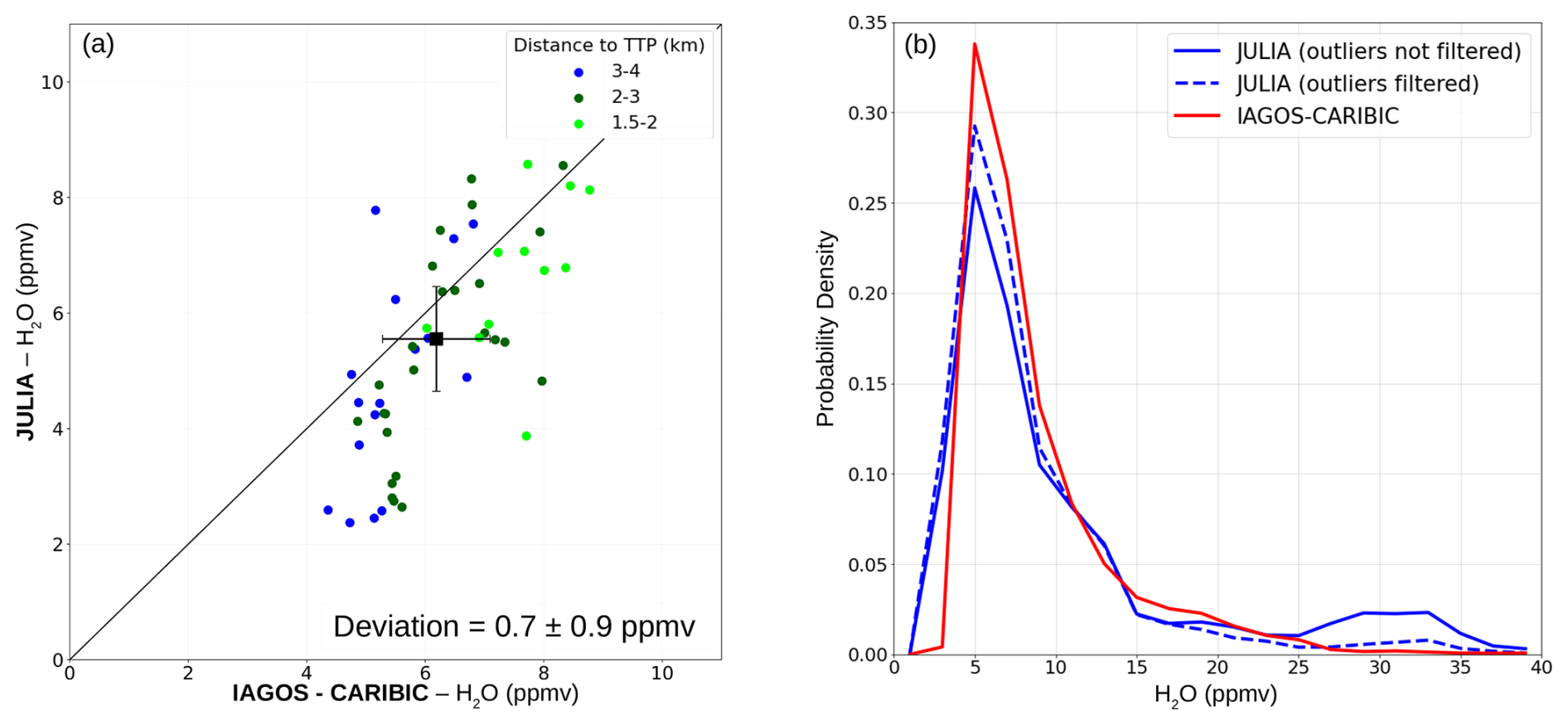
Figure 4 Statistical intercomparison of IAGOS-CARIBIC with JULIA H₂O. (a) LMS H₂O mixing ratios of IAGOS-CARIBIC vs. JULIA, calculated based on the methodology described in Sect. 3.1 and 3.2; the colour code denotes the distance to the TTP (see legend). The mean bias and the corresponding standard deviation based on all sampling bins is indicated by the black dot and the bar, respectively. (b) Based on single measurements from all sampling bins in (a), the frequency distribution is shown both with and without the filtering of strong outliers.

Systematic differences can be found for sampling bins where JULIA indicates H₂O of less than 6 ppmv. Bins with JULIA indicating H₂O of less than 3.5 ppmv are related to polar air masses during one specific campaign, POLARCAT (Polar Study using Aircraft, Remote Sensing, Surface Measurements and Models, of Climate, Chemistry, Aerosols, and Transport). It is not unlikely that these are cases of unusually low H₂O that were purposefully measured during certain campaign flights and meteorological conditions and are thus over-represented in JULIA. When filtering out data from that specific campaign, the bias between the two datasets gets less pronounced. However CARIBIC data are still moister by 0.5–1 ppmv for mixing ratios below 6 ppmv (see all bins with JULIA indicating >3.5 ppmv in Fig. 4a), which is outside the stated uncertainty of the JULIA and CARIBIC data (see Table 1). It cannot be argued whether this small mean deviation is a result of different atmospheric sampling strategies between campaign and commercial aircraft flights, despite the strict filter conditions, or a small systematic bias. Nevertheless, the possibility of a moist bias at the very dry end must be considered in the comparison between CARIBIC and MOZAIC&CORE, which is presented in the next section.

3.3 Evaluation of IAGOS-MOZAIC&CORE H₂O

Figure 5 displays the intercomparison of the sampled mean values of $\stackrel{\mathrm{‾}}{{\text{RH}}_{\text{liq}}},\stackrel{\mathrm{‾}}{{\text{RH}}_{\text{ice}}}$ and $\stackrel{\mathrm{‾}}{{\mathrm{H}}_{\mathrm{2}}\mathrm{O}}$ (Eq. 2) with respect to the season and the distance to the tropopause. Additionally, Fig. A1 shows the same plots but the data being sampled into 5 K means instead of being averaged over all temperature ranges. MOZAIC and CORE are treated separately to examine the agreement between them. A majority of the measurements contributing to the sampled mean values originate from the extra-tropics between 30 and 80° N, for which this intercomparison is valid. For the reference dataset CARIBIC, in the uncertainty of $\stackrel{\mathrm{‾}}{{\text{RH}}_{\text{liq}}}$ and $\stackrel{\mathrm{‾}}{{\text{RH}}_{\text{ice}}}$, uncertainties of H₂O (4 %), temperature (0.7 K; Benjamin et al., 1999) and pressure (1 hPa; Tang et al., 2005) are incorporated. The resulting relative bias of the CARIBIC sampling bins is on the order of 7 %.

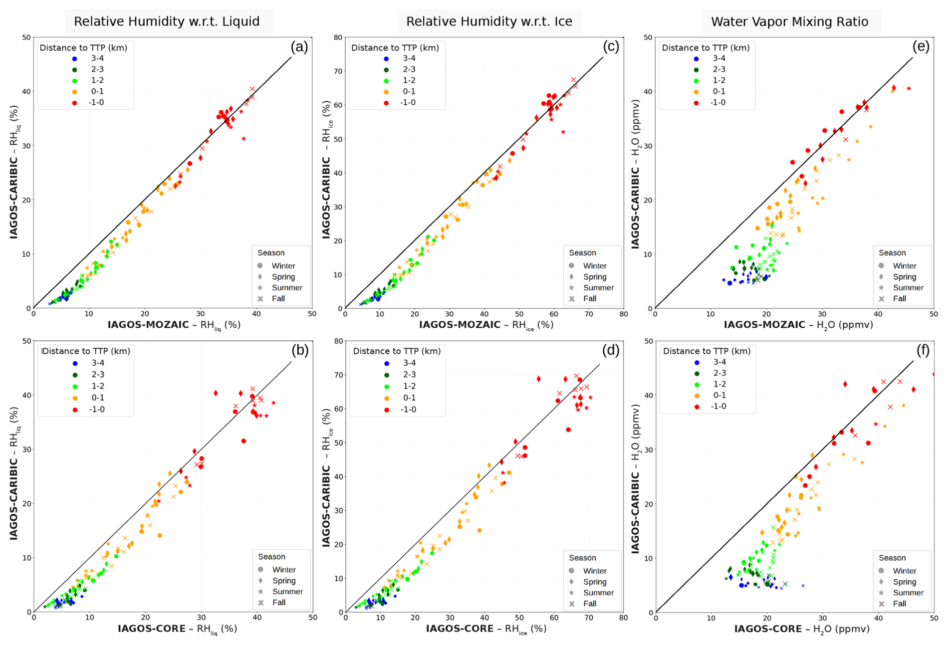
Figure 5 Statistical intercomparison of H₂O from IAGOS-MOZAIC&CORE with IAGOS-CARIBIC. Sampling bin means of $\stackrel{\mathrm{‾}}{{\text{RH}}_{\text{liq}}}$ (a, b), $\stackrel{\mathrm{‾}}{{\text{RH}}_{\text{ice}}}$ (c, d) and $\stackrel{\mathrm{‾}}{{\mathrm{H}}_{\mathrm{2}}\mathrm{O}}$ (e, f) for IAGOS-MOZAIC (a, c, e) and IAGOS-CORE (b, d, f) vs. IAGOS-CARIBIC. The sampling bins are derived following the methodology described in Sect. 3.1; the colour code denotes the distance to the tropopause and the symbols the corresponding season.

In the comparison of MOZAIC to CARIBIC data, a distinct relationship is observed. When examining bins below the TTP where $\stackrel{\mathrm{‾}}{{\text{RH}}_{\text{liq}}}$ values are mostly above 30 %, MOZAIC and CARIBIC show a good agreement. This agreement is attributed to the infrequent occurrence of dry conditions with low RH_liq which tend to be biased. Figure 6a illustrates the correlation between the relative number of MOZAIC measurements below 10 % RH_liq, which was stated to be the upper limit for which ICH data show good quality by Neis et al. (2015a), and the bias between MOZAIC and CARIBIC. Notably, the bias is prominent when the number of measurements below 10 % RH_liq is higher than 20 % (Fig. 6a), while bins with fewer measurements below 10 % RH_liq show little to no significant biases. However, it cannot be verified from our analyses where the upper limit is situated above which the measurements are of good quality.

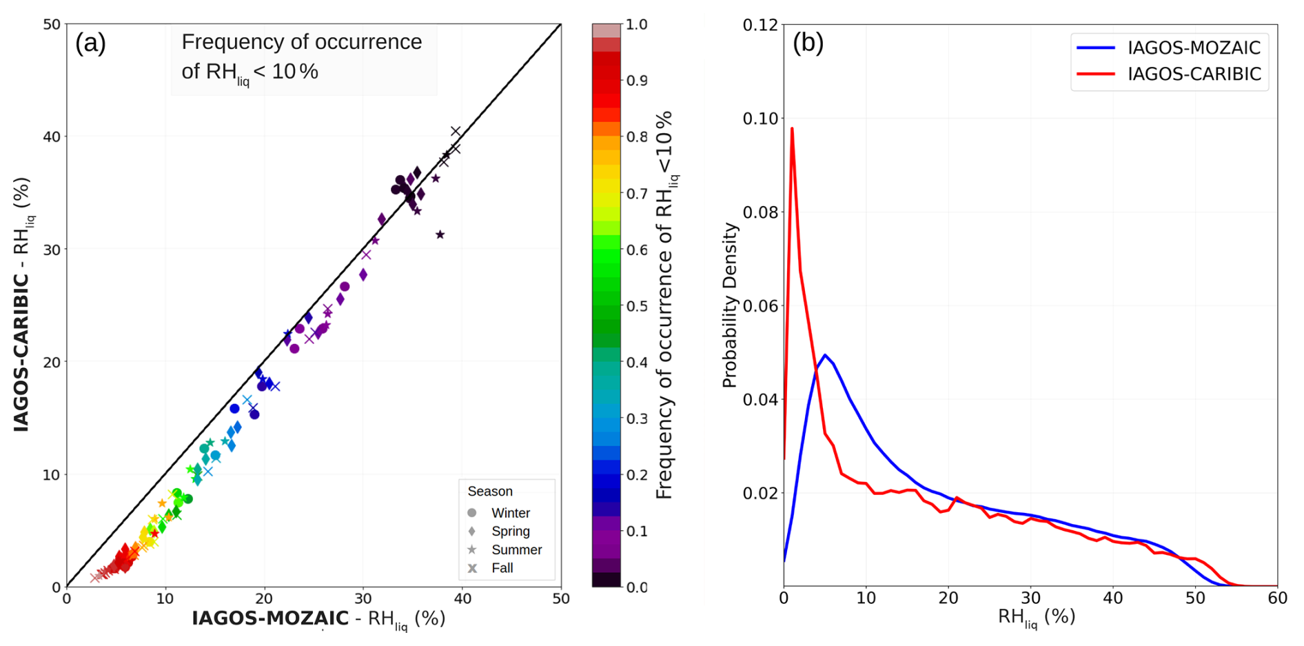
Figure 6 (a) For IAGOS-MOZAIC, the plots show the same sampling bins as in Fig. 5. The colour code indicates the frequency of occurrence of single measurements below a threshold of 10 % by IAGOS-MOZAIC that contribute to the shown mean values. (b) Occurrence frequencies of RH_liq for CARIBIC and MOZAIC, based on all data that go into the sampling bins in (a).

For MOZAIC and CARIBIC, Fig. 6b presents the PDFs constructed from all measurements included in the sampling bins of Fig. 6a. The PDFs in panel (b) exhibit a similar pattern for RH_liq values above 20 %, but they diverge significantly below this threshold, suggesting that ICH RH_liq might be biased for values under 20 %. However, the observed discrepancy in the RH_liq>10 % range could also reflect a scenario where no consistent bias exists across specific RH_liq ranges. Instead, a broad distribution of measurements around a biased mean state may be present. In such a case, a mean moist bias for a given RH_liq range would increase the PDF's representation of RH_liq values at higher levels.

Non-linear bias behaviour could be attributed to uncertainties in the calibration the sensor's offset drift, which occurs between the routine ICH calibrations conducted every 3 months (Petzold et al., 2020). Although an in-flight calibration is performed to account for this sensor drift (Smit et al., 2008), uncertainties in the process (as noted in Smit et al., 2008) can introduce non-linear variations in the bias of individual measurements between calibration intervals. Consequently, while this intercomparison study cannot determine the behaviour of the bias for individual measurements, it does provide insights into the bias of mean values used in climatological studies.

The sampling bins with $\stackrel{\mathrm{‾}}{{\text{RH}}_{\text{liq}}}$ values below 20 % exhibit significant systematic moist biases, with relative differences of 100 % or more for $\stackrel{\mathrm{‾}}{{\text{RH}}_{\text{liq}}}$ of 10 % and less. For layers closer to the TTP, there is a lower but still noteworthy bias. During summer, certain bins have $\stackrel{\mathrm{‾}}{{\text{RH}}_{\text{liq}}}$ values of 15 % or less already in the first kilometre above the TTP, whereas the same levels relative to the TTP during other seasons indicate much higher values. This seasonality is attributed to the higher temperatures observed in the respective sampling bins during the summer season, and biases of the mean values are in the range of only about 1 % to 3 % RH_liq during this season close to the TTP.

For the comparison of CORE and CARIBIC, we used data between 2018 and 2022 only. This specific time frame was chosen because before 2018, a grounding issue between the sensor and the data acquisition unit caused a large noise on the signal and thus a reduced quality flag of the data. Therefore, we decided to utilise only data with the highest quality unaffected by this issue.

On average, the comparison of CORE and CARIBIC shows similar mean biases in the LMS, similar to what the comparison with MOZAIC revealed. However, for CORE, there is a stronger variation in the bin mean values compared to MOZAIC, which can be attributed to differences in the temporal coverage (2018–2022 and 1995–2022) of CORE and CARIBIC, respectively, due to the large year-to-year variability in UT/LMS H₂O (Kunz et al., 2008).

4 Adjustment of IAGOS-MOZAIC&CORE LMS H₂O to IAGOS-CARIBIC

4.1 Adjustment methodology

Following the mapping approach outlined in Sect. 3.1, the next step is to apply an algorithm to adjust the biased MOZAIC&CORE H₂O data using CARIBIC H₂O as a reference. A fixed bias for individual measurements, however, cannot be defined as a function of RH_liq due to the sensor offset drift at 0 % RH_liq (see Sect. 3.3). As a result, it is also not feasible to directly adjust ICH data from IAGOS flights using data from campaign flights equipped with ICH and high-precision H₂O instruments, like FISH.

Given the limitations mentioned above, the primary objective of our methodology is to adjust the sampling bin mean values $\stackrel{\mathrm{‾}}{{\text{RH}}_{\text{liq}}}$. These mean values, based on thousands of individual measurements, represent a climatological state. One potential approach is to align the probability density functions (PDFs) of the MOZAIC&CORE data with those of the reference dataset (CARIBIC; see Fig. 6b for illustration). However, because CARIBIC has fewer measurements, the PDFs for its sampling bin mean values are noisier and more variable, making it difficult to directly match the distributions. As a result, we pursue an alternative approach: analysing how the probability distribution function of the data influences the mean bias and adjusting accordingly. The steps of the approach are described below.

1. Segmenting the distribution and analysing the bias by frequency of occurrence (FO). We divide the RH_liq frequency distribution of each sampling bin into smaller segments. For each segment, we compute the frequency of occurrence (FO) of values falling below specific RH_liq thresholds (FO thresholds =0.5 %–15 % RH_liq, with step size of 0.5 %). This allows us to determine how often certain RH_liq values occur in the distribution. As an example, in Fig. 6a, the FO for the 10 % threshold is shown. Figure 7a illustrates this concept for a distribution having a mean $\stackrel{\mathrm{‾}}{{\text{RH}}_{\text{liq}}}$ of 6 %, with the blue lines indicating two specific RH_liq thresholds: RH_liq<3.5 % and RH_liq<4.5 %.

   We perform this segmentation for the distributions of all MOZAIC&CORE sampling bins that fall in between certain $\stackrel{\mathrm{‾}}{{\text{RH}}_{\text{liq}}}$ ranges, with a step size of 1 % RH_liq ($\stackrel{\mathrm{‾}}{{\text{RH}}_{\text{liq}}}=\mathrm{0.5}$ %–1.5 %, 1.5 %–2.5 %, …). For each of the bins in the respective $\stackrel{\mathrm{‾}}{{\text{RH}}_{\text{liq}}}$ ranges, the bias to the CARIBIC sampling bins is calculated. Next, we also consider the different FO thresholds and sort the biases as a function of the number of measurements falling below these thresholds. For the two RH_liq thresholds indicated in Fig. 7a (dashed blue lines) and based on all sampling bins with $\stackrel{\mathrm{‾}}{{\text{RH}}_{\text{liq}}}$ in the range of 5.5 %–6.5 %, Fig. 7c and d display the respective biases as a function of the FO (y axis; blue dots). Similar plots for $\stackrel{\mathrm{‾}}{{\text{RH}}_{\text{liq}}}=\mathrm{15}$ % are presented in Fig. A2.

2. Derivation of a mean bias as a function of $\stackrel{\mathrm{‾}}{{\text{RH}}_{\text{liq}}}$ and FO. A regression (black dots in Fig. 7c and d) is applied to the correlation between all biases and FO fulfilling the RH_liq threshold. The deviations from the regression are on the order of ±0.5 % RH_liq and thus a robust approximation. By performing this method for various ranges of $\stackrel{\mathrm{‾}}{{\text{RH}}_{\text{liq}}}$, we obtain a series of mean biases as a function of both percent RH_liq thresholds and the corresponding FO. This enables us to study how the bias varies as a function of the distribution of data points.

3. Interpolation and construction of look-up tables for bias correction. Once the mean biases (black dots) for different FO thresholds are calculated, we apply an interpolation to smooth the fluctuations between the bias values for different $\stackrel{\mathrm{‾}}{{\text{RH}}_{\text{liq}}}$ ranges. This step is necessary to minimise the effects of distribution uncertainties, leading to more consistent and reliable corrections. The result is a set of look-up tables containing the corrected mean values for specific $\stackrel{\mathrm{‾}}{{\text{RH}}_{\text{liq}}}$ values and the corresponding FO thresholds. An example of such a look-up table for $\stackrel{\mathrm{‾}}{{\text{RH}}_{\text{liq}}}=\mathrm{6}$ % is shown in Fig. 7b, where the black boxes highlight the biases corresponding to the two thresholds shown in Fig. 7c and d.

4. Final bias calculation and adjustment. The final adjusted mean bias is derived by calculating the arithmetic mean of the biases at different FO thresholds. The equation for the final mean bias is given by

   $$\begin{array}{}\text{(3)}& {\displaystyle }{\displaystyle }\stackrel{\mathrm{‾}}{\mathrm{\Delta }{\text{RH}}_{\text{liq}}}={\displaystyle \frac{\mathrm{1}}{n}}\sum _{i=\mathrm{0}}^n\mathrm{\Delta }{\text{RH}}_{\text{liq}}\left[i\right],\end{array}$$

   where n represents the number of FO thresholds. As an example, the biases for different RH_liq FO thresholds are illustrated by the grey dots in Fig. 7b. The final mean bias, $\stackrel{\mathrm{‾}}{\mathrm{\Delta }{\text{RH}}_{\text{liq}}}$, is obtained by averaging all the individual biases. This approach ensures that we account for the biases associated with various FO thresholds, leading to a more comprehensive and accurate adjustment of the mean RH_liq values.

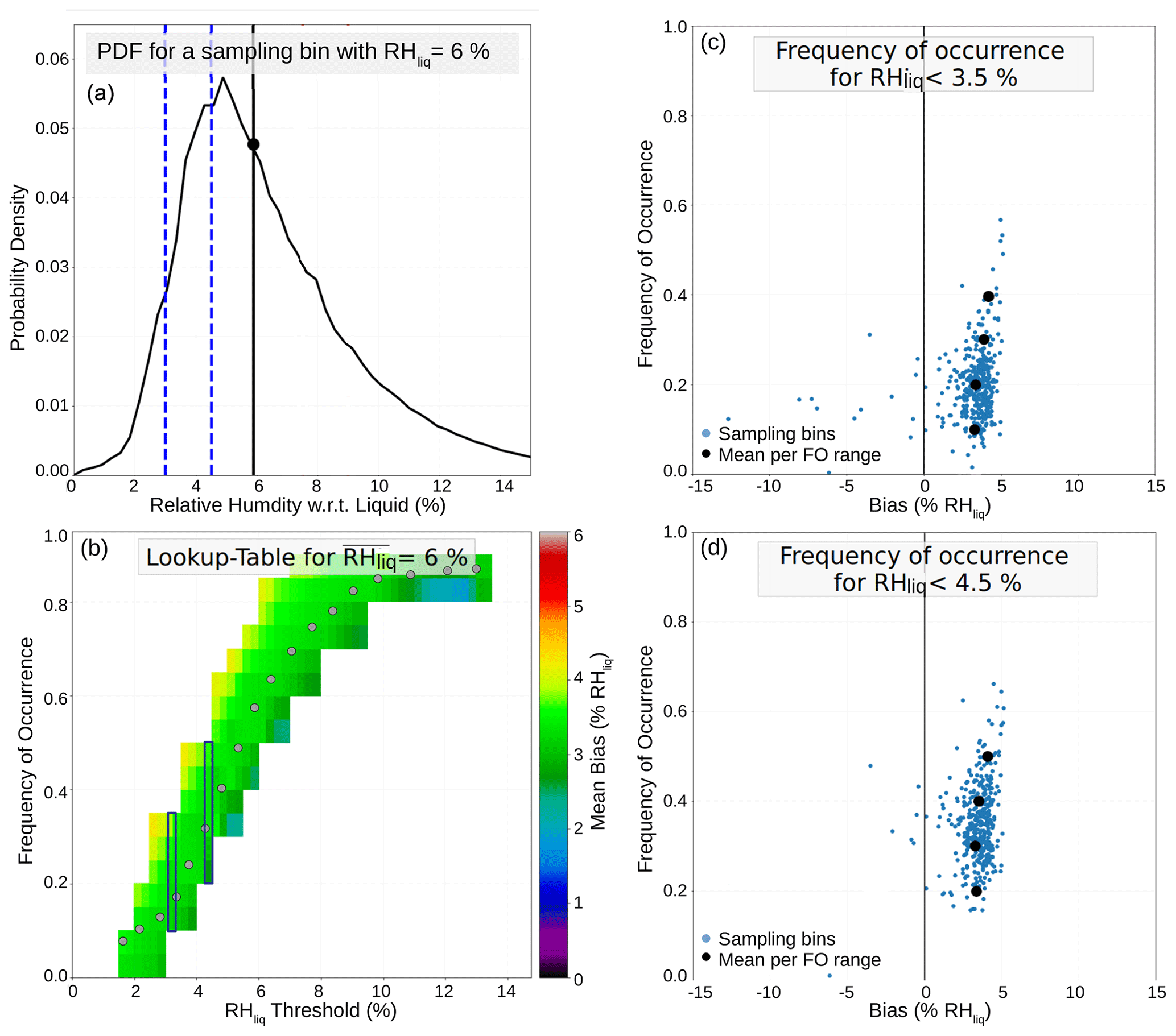
Figure 7 Application example of the IAGOS adjustment algorithm. (a) Example RH_liq frequency distribution of a sampling bin with a mean of $\stackrel{\mathrm{‾}}{{\text{RH}}_{\text{liq}}}=\mathrm{6}$ %. For this mean value, (b) shows the look-up table with the values used as adjustment based on different RH_liq thresholds and the corresponding cumulative distribution (y axis). For the two thresholds indicated by the dotted blue lines in (a), the plots (c) and (d) show the derivation of the mean bias (black dots) based on the weighted mean of the sampled mean values (blue dots).

When the adjustment algorithm is applied to the entire MOZAIC dataset, using the sampled mean values shown in Fig. 5, the corrected values exhibit a good agreement with the CARIBIC data, as shown in Fig. 8a. The adjusted MOZAIC values now cluster closely around the 1-to-1 line, without any obvious bias. Furthermore, Fig. 8b presents vertical profiles of H₂O from MOZAIC (blue), CORE (black), CARIBIC (red) and JULIA (green) during the winter and spring seasons in the 40–60° N latitudinal region. At altitudes of 1 km and more above the TTP, where MOZAIC&CORE exhibited significant biases, the adjusted mean values now align well with the reference data (CARIBIC and JULIA). This confirms that the adjustment methodology is effective and provides reliable mean values across different seasons.

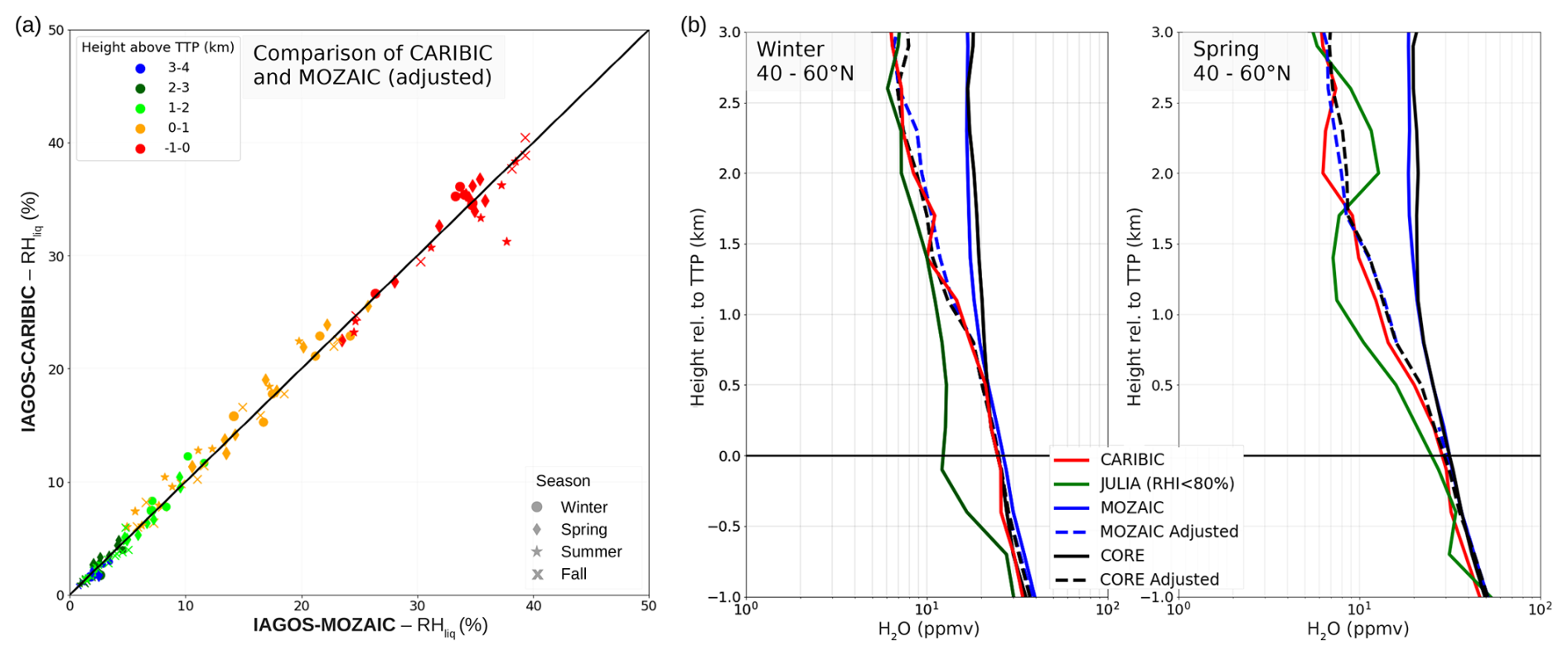
Figure 8 Application of the adjustment algorithm on the IAGOS data. Panel (a) shows a comparison of the same sampling bins between IAGOS-MOZAIC and IAGOS-CARIBIC as shown in Fig. 6 but with the adjustment algorithm applied to the mean values. Panel (b) shows two mean vertical UT/LMS H₂O profiles of IAGOS-CARIBIC, JULIA and IAGOS-MOZAIC&CORE (adjusted and unadjusted).

4.2 Application and uncertainties of adjusted IAGOS-MOZAIC&CORE H₂O

4.2.1 Uncertainty estimate

While the adjustment improves the agreement between the MOZAIC&CORE and CARIBIC datasets, several sources of uncertainty remain. These include the following.

• Measurement uncertainties. In CARIBIC, uncertainties in the RH_liq derivation (from H₂O, temperature and pressure measurements) introduce a relative bias of about 7 % (see Sect. 3.2.2).

• Method uncertainty. The small number of CARIBIC measurements and differences in the temporal and geographical coverage of the datasets can lead to uncertainties. However, the sampling strategy designed in this study helps reduce such uncertainties.

The method uncertainty is determined like the following: the bias derivation (see Fig. 7) is also performed for each season separately. In the next step, the standard deviation for each bias as a function of $\stackrel{\mathrm{‾}}{{\text{RH}}_{\text{liq}}}$ and FO (see last section) is derived from the four seasonal means and, from these deviations, the mean standard deviation as a function of just $\stackrel{\mathrm{‾}}{{\text{RH}}_{\text{liq}}}$. The mean bias (averaged over all FO) as a function of unadjusted $\stackrel{\mathrm{‾}}{{\text{RH}}_{\text{liq}}}$ is shown in Fig. 9 (dashed line), with the red area indicating the uncertainty due to the adjustment method and the blue area the additional uncertainty when measurement uncertainties are also taken into account. The uncertainty of the derived adjusted $\stackrel{\mathrm{‾}}{{\mathrm{H}}_{\mathrm{2}}\mathrm{O}}$ varies depending on the corresponding $\stackrel{\mathrm{‾}}{\text{RH}{}_{\text{liq}}}$. During summer, $\stackrel{\mathrm{‾}}{\text{RH}{}_{\text{liq}}}$ in the LMS tends to be lower due to higher temperatures compared to winter, with lower $\stackrel{\mathrm{‾}}{\text{RH}{}_{\text{liq}}}$ having higher relative uncertainties. Based on all $\stackrel{\mathrm{‾}}{\text{RH}{}_{\text{liq}}}$ in the extra-tropical LMS, Fig. 9b and c show the mean uncertainty and the 10 %–90 % percentiles (dashed line and shaded area, respectively). For 10 ppmv for example, the mean bias (bias range) is 1.0 (0.8–2.3) and 2.4 (2.0–3.1) ppmv for winter and summer, respectively.

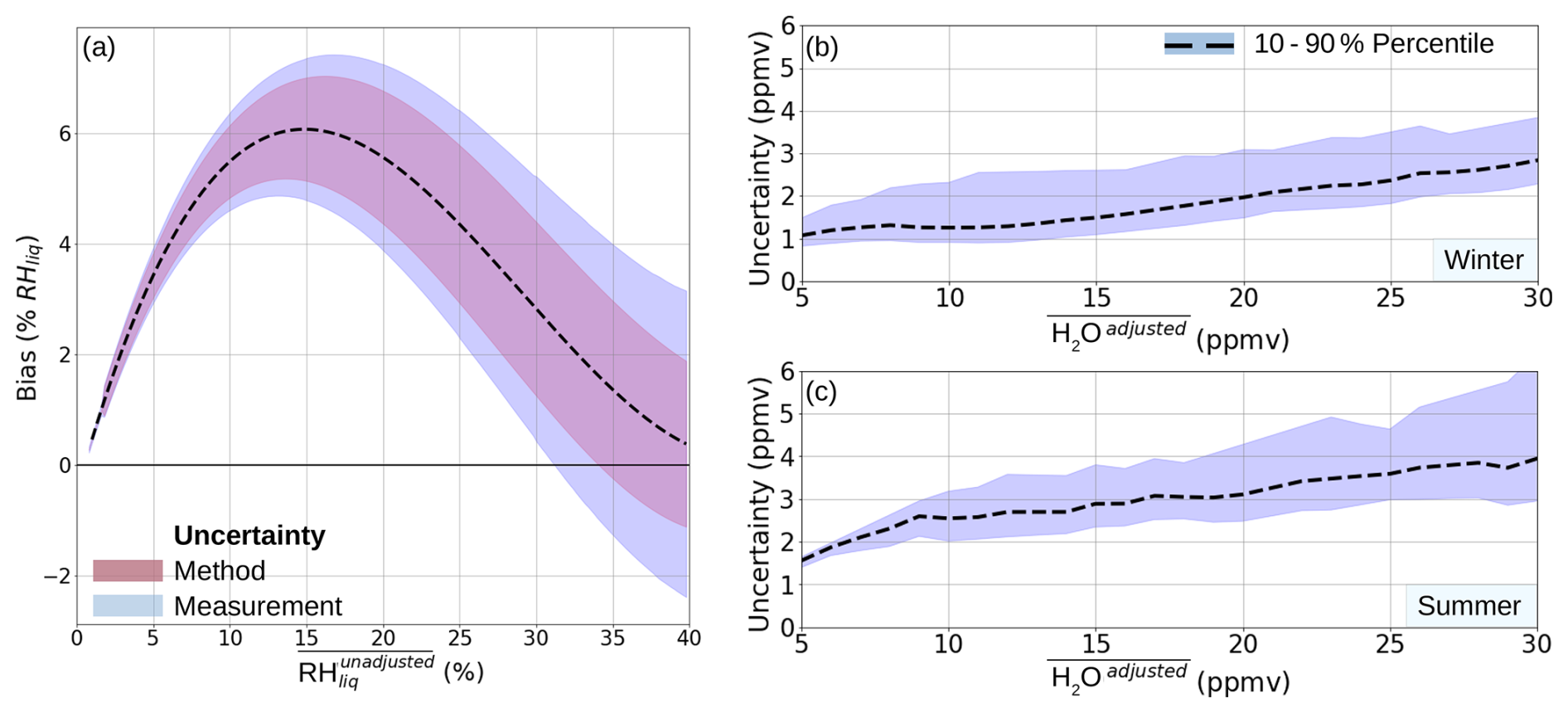
Figure 9 Error budget. (a) Mean bias derived from the mean of all FO thresholds as a function of $\stackrel{\mathrm{‾}}{{\text{RH}}_{\text{liq}}}$ (dashed line) and the uncertainty estimate due to the adjustment method (red shaded) and due to measurement uncertainties (blue shaded). (b, c) For $\stackrel{\mathrm{‾}}{{\mathrm{H}}_{\mathrm{2}}\mathrm{O}}$ derived from adjusted $\stackrel{\mathrm{‾}}{{\text{RH}}_{\text{liq}}}$, the mean bias (dashed line) and the 10 %–90 % percentiles (blue shaded) is shown for winter (b) and summer (c).

4.2.2 Application

The adjusted MOZAIC&CORE-based H₂O climatology offers the advantage of a longer record and greater spatial and seasonal sampling than the datasets of CARIBIC and JULIA, enabling more detailed analysis of the drivers of H₂O variability. However, the adjustment of mean values requires a sufficient number of measurements in order to provide a smooth PDF based on which the adjustment is performed. In the lower stratosphere (LS), variability in H₂O increases with altitude towards the tropopause, necessitating a larger number of measurements to ensure the PDF is not skewed by outliers.

To determine the necessary number of measurements, a Kolmogorov–Smirnov test (Berger and Zhou, 2014) is performed. This test assesses whether the data fits a specific distribution, typically a Weibull distribution for the IAGOS RH_liq data, with at least 95 % confidence. For the sampling strategy outlined in this study (Sect. 3.1), the required number of data points ranges from approximately 300 (LMS; Δz>2 km) to 1000 (UT).

Due to the requirement for a substantial amount of data and the relative uncertainty exceeding 10 % in the driest range, robust trend analysis cannot be reliably performed using the derived dataset. Even in regions with sufficient data availability, the level of uncertainty is greater than the potential magnitude of H₂O trends.

4.3 Adjusted UT/LMS H₂O climatologies

Multi-annual monthly means of adjusted H₂O, based on all MOZAIC&CORE data, are shown in Fig. 10 for two Θ levels: 335 K (a–d) and 350 K (e–h). The solid magenta line indicates the mean 2 PVU line. The H₂O data are provided at a resolution of at least 5 ppmv. This relatively low resolution was chosen in regard of the uncertainties in the adjusted dataset. Specifically, for values below 20 ppmv, the uncertainty of the adjusted data can reach up to 30 %. Therefore, a higher resolution would not be meaningful. Nonetheless, the given resolution is sufficient to capture spatial and seasonal features, also in areas where CARIBIC data are sparse or unavailable due to limited flight coverage (see discussion below).

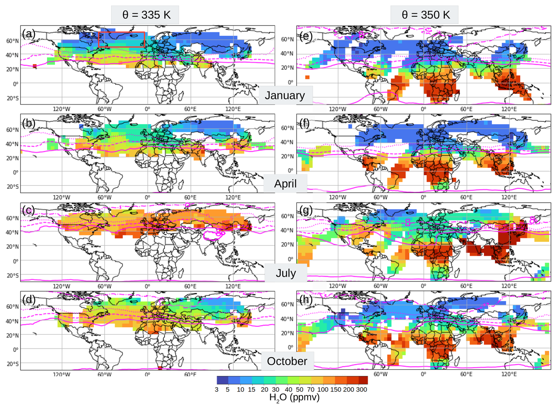
Figure 10 H₂O mixing ratio climatologies. Monthly means (January, April, July and October) for two Θ level. In magenta and shown with solid, dashed, dotted and dash-dotted lines, the mean position of the 2, 4, 6 and 8 PVU line is indicated. The red box in (a) highlights the region further investigated in Fig. 11.

Over parts of North America as well as southeast Asia, the monsoon-related H₂O increase during the Northern Hemisphere summer season (Nützel et al., 2019) is evident at Θ=350 K (Fig. 10g), i.e. at a Θ level that corresponds to subtropical and tropical air masses at passenger aircraft altitude over these regions. Here, mean values are by a factor of 3 (North America) to 10 (southeast Asian) higher compared to other regions at the same geographic latitudes.

From fall to spring the highest values in the mid-latitudes at 335 K can be found over the North Atlantic. Higher H₂O amounts occur over the Atlantic than over continental regions during the winter half of the year, associated with greater low-pressure activity over this area, and the resulting large-scale uplift of moist and relatively warm air masses (UT) and potential isentropic mixing of moisture into the LS. Enhanced isentropic mixing into the LS over the Atlantic was found to occur in relation to warm conveyor belt outflow (Kunkel et al., 2019), based on measurements during the WISE (Wave-driven ISentropic Exchange) campaign.

For the North Atlantic (50–70° N and 5–65° W), Fig. 11a–d show adjusted $\stackrel{\mathrm{‾}}{{\mathrm{H}}_{\mathrm{2}}\mathrm{O}}$ climatologies, given in coordinates of equivalent latitude and potential temperature difference relative to the TTP (ΔΘ). Close to the TTP (±20 K), a strong annual H₂O cycle can be observed. Along the TTP, the H₂O varies between 20–30 ppmv (winter; Θ=315–325 K), and 100 ppmv (summer; Θ=325–340 K). Investigating the annual cycle along isentropic levels in the LMS, at 340 K, a distinct increase during the summer half of the year can be found. During January, H₂O is in the range of 5–20 ppmv and increases to 15–70 ppmv during July, with a strong gradient along Δφ_EQ ranges. This pattern can strongly be related to the increase in the tropopause Θ level during summer and the subsequently stronger influence of (isentropic) transport of H₂O from the subtropical regions into the mid-latitude LMS. Generally, layers in the LMS close to the TTP (ΔΘ<10 K) are moister during the summer season. A key question here is to what extent this increase can be attributed to local transport from the underlying upper troposphere (UT) or to large-scale transport, particularly from monsoon-influenced regions. Further trajectory-based analysis is essential to quantify the contributions of the different transport mechanisms involved.

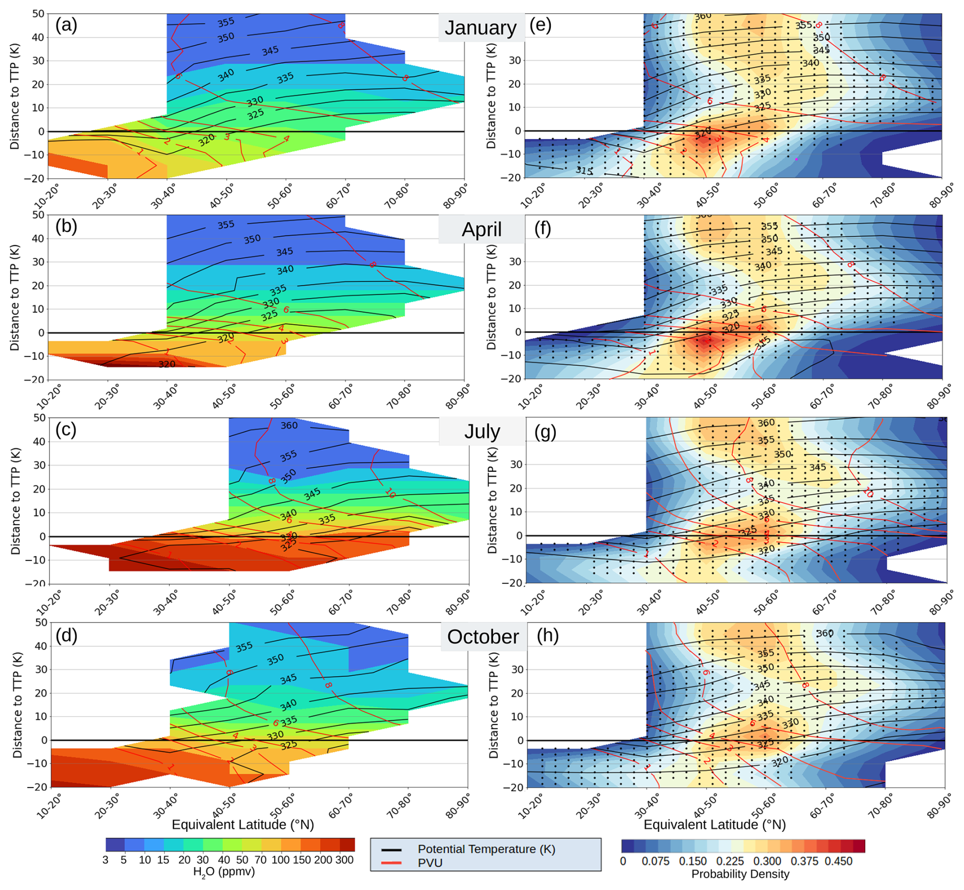
Figure 11 Adjusted UT/LMS H₂O mixing ratio climatology for the North Atlantic region (50–70° N and 5–65° W). Panels (a)–(d) show the multi-annual monthly means of the adjusted H₂O. (e–h) Occurrence frequency of sampling bins of equivalent latitude and potential temperature difference (ΔΘ) to the TTP (the resolution is 5 K and normalised per ΔΘ range). The black dots indicate sampling bins for which MOZAIC&CORE provide data from at least 20 flights.

At levels of ΔΘ of around 20 K above the TTP, the highest values can be found during fall, with a maximum during October (Fig. 11d), in contrast to a slight decrease from summer to fall in the LMS close to the TTP (ΔΘ<10 K) and in the UT (Fig. 11c and d). An increase in the exTL height during the fall season is a well-known feature for the northern extra-tropics, as reported in various studies (e.g. Zahn et al., 2014). The reasons for the seasonal variability described in this section are not aimed to be discussed in detail in this paper (however, see e.g. Gettelman et al., 2011; Zahn et al., 2014) but will be the focus of future publications based on the adjusted MOZAIC&CORE climatologies.

Finally, we examine how well the climatology shown in Fig. 11a–d covers the UT/LMS over the North Atlantic, given that passenger aircraft fly at constant altitudes and might avoid certain weather conditions. In order to investigate this, a sampling of ΔΘ and Δφ_EQ is applied to the ERA5 data. The probability density (normalised per ΔΘ) based on ERA5 data from all vertical levels is shown in Fig. 11. The dotted areas in the plots illustrate the sampling bins where IAGOS provides data from at least 20 flights. Overall, good coverage is found. During winter and spring, only air masses in the UT below $\mathrm{\Delta }\mathrm{\Theta }=-\mathrm{15}$ K are not well covered (Fig. 11a and b). During summer and fall (Fig. 11d and e), air masses with an equivalent latitude of 30–40° N, i.e. of subtropical origin, are mostly not covered in the LMS, which accounts for 20 %–30 % of all air masses. However, the most frequent air masses (Δφ_EQ=50–80° N) are covered by IAGOS also during the summer season.

5 Conclusion and outlook

This study presented an algorithm to produce adjusted water vapour (H₂O) mean values in the lowermost stratosphere (LMS) based on measurements of the compact IAGOS capacitive humidity sensor (ICH) operating on board MOZAIC&CORE to the sophisticated measurements from IAGOS-CARIBIC. First, a statistical comparison of MOZAIC&CORE with CARIBIC H₂O was conducted, selecting CARIBIC as the reference dataset due to its advanced instrumentation and similar spatial and temporal distribution. Although CARIBIC has a limited number of about 500 flights compared to around 60 000 flights by MOZAIC&CORE combined, it still provided a sufficient number of measurements for a valid intercomparison in the extra-tropical Northern Hemisphere.

For the comparison, a mapping approach was utilised where measurements were sampled into bins of similar dynamical origin and properties. Considerations of equivalent latitude, season and height relative to the tropopause were used to derive corresponding mean RH_liq values ($\stackrel{\mathrm{‾}}{{\text{RH}}_{\text{liq}}}$). Initially, CARIBIC data were compared with high-precision campaign measurements summarised in the JULIA database. It was demonstrated that the CARIBIC H₂O instrument package can quantify low stratospheric H₂O concentrations of 10 ppmv or less, making them suitable for intercomparison with MOZAIC&CORE. However, it has to be regarded that JULIA and IAGOS measurements were, on average, conducted during different atmospheric conditions. While campaign flights often tend to take place during specific atmospheric conditions, passenger aircraft flights tend to avoid convective systems and other conditions with a turbulent character (e.g. frontal systems). Consequently, JULIA data were excluded from the comparison and adjustment of MOZAIC&CORE, as including them might introduce greater uncertainties rather than providing additional benefits from having more data.

The comparison between MOZAIC&CORE with CARIBIC showed good agreement in the (extra-tropical) upper troposphere. However, above the tropopause, the average values were generally biased, with the magnitude of the bias increasing with distance above the tropopause, reaching relative differences of 300 % for H₂O at around 5 ppmv. This systematic bias in the lower stratosphere was attributed to limitations of the ICH sensor, which loses sensitivity below approximately 10 % RH_liq. Despite this, the sensors consistently performed well for mean values above 30 ppmv.

Subsequently, using the mapping approach, a method was developed to adjust $\stackrel{\mathrm{‾}}{{\text{RH}}_{\text{liq}}}$ from MOZAIC&CORE to those from CARIBIC. The biases were quantified as a function of $\stackrel{\mathrm{‾}}{{\text{RH}}_{\text{liq}}}$, enabling the adjustment of MOZAIC&CORE H₂O climatologies with an uncertainty of approximately 1 ppmv (winter) to 2.5 ppmv (summer) for mean values of 10 ppmv and less.

A caveat is that the adjustment of $\stackrel{\mathrm{‾}}{{\text{RH}}_{\text{liq}}}$ is based on a statistical comparison of the small CARIBIC reference dataset with the much larger MOZAIC&CORE dataset. This introduces a small systematic error due to the limited representativeness of the CARIBIC dataset. This representativeness error could be neglected for studies of variability and transport processes, but for H₂O trend analyses this error must be considered and quantified. Nevertheless, due to the lack of in situ measurements in the UT/LMS, the adjusted climatologies provide better resolution of temporal and spatial variability in UT/LMS H₂O compared to other in situ or space-borne datasets. This will contribute to a better understanding of the H₂O variability in the extra-tropical UT/LMS and its connection to various transport and mixing processes. Based on the adjusted H₂O climatologies, upcoming studies will investigate the contribution of different transport mechanisms to the H₂O variability, using backward trajectories and simulations of (de-)hydration of air masses along their pathways. This enhanced understanding of the H₂O variability and its corresponding transport mechanisms is crucial for improving the quality of model simulations concerning current and future H₂O concentrations in the UT/LMS and their impact on the radiative forcing in a warming climate.

Appendix A

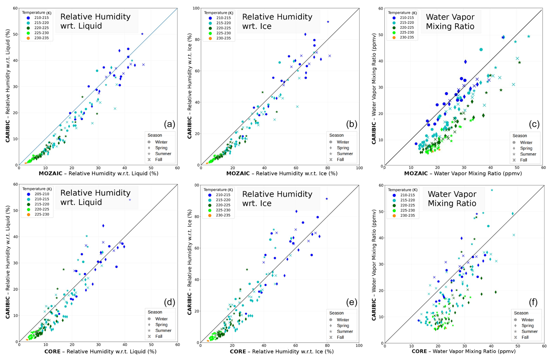
Figure A1 Intercomparison of sampled mean values of RH_liq, RH_ice and H₂O for IAGOS-MOZAIC (a–c) and CORE (d–f) with IAGOS-CARIBIC. Instead of the height relative to the tropopause as shown in Fig. 5, the colours indicate temperature ranges.

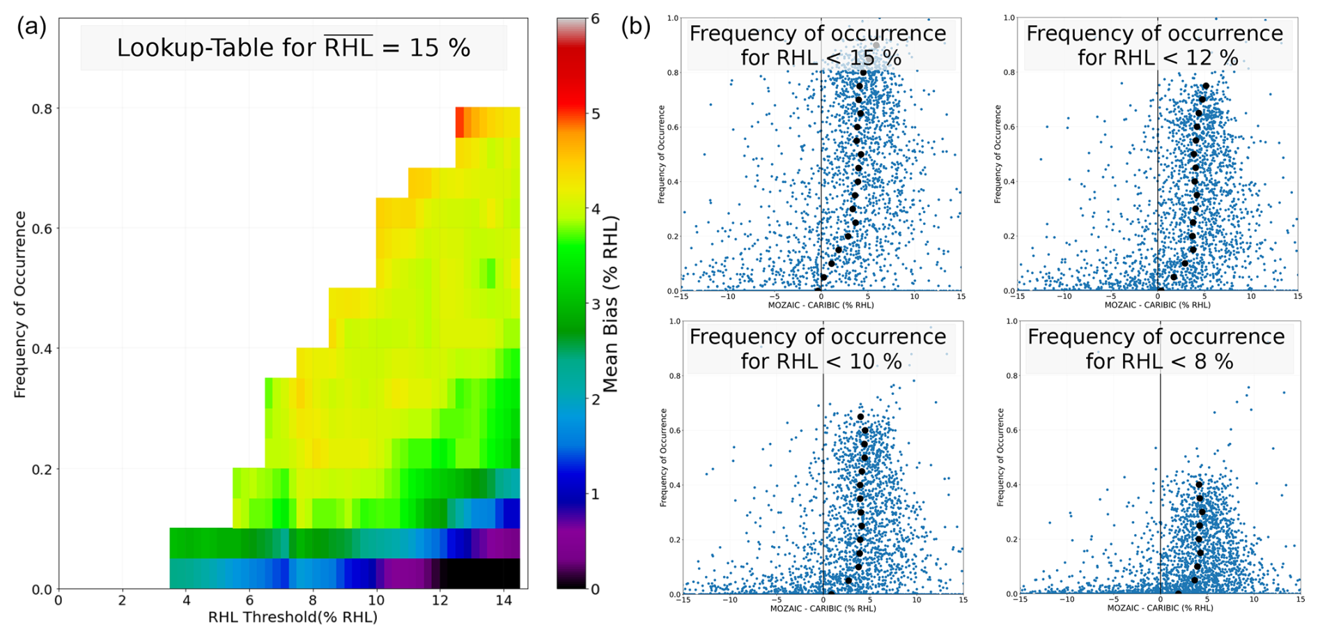
Figure A2 (a) Look-up table for a mean value $\stackrel{\mathrm{‾}}{{\text{RH}}_{\mathrm{L}}}$ of 15 % which will be used to adjust potentially biased mean values of 15 %. (b) Corresponding frequency of occurrence for exemplary thresholds that are the basis for the final look-up table.