Driving factors of aerosol acidity: a new hierarchical quantitative analysis framework and its application in Changzhou, China

Aerosol acidity (or pH) plays a crucial role in atmospheric chemistry, influencing the interaction of air pollutants with ecosystems and climate. Aerosol pH shows large temporal variations, while the driving factors of chemical profiles versus meteorological conditions are not fully understood due to their intrinsic complexity. Here, we propose a new framework to quantify factor importance, which incorporated an interpretive structural modeling (ISM) approach and time series analysis. In particular, a hierarchical influencing factor relationship is established based on the multiphase buffer theory with ISM. A long-term (2018–2023) observation dataset in Changzhou, China, is analyzed with this framework. We found the pH temporal variation is dominated by the seasonal and random variations, while the long-term pH trend varies little despite the large emission changes. This is an overall effect of decreasing PM_2.5, increasing temperature and increased alkali-to-acid ratios. Temperature is the controlling factor of pH seasonal variations, through influencing the multiphase effective acid dissociation constant $K_{\mathrm{a}}^{\ast }$, non-ideality c_ni and gas–particle partitioning. Random variations are dominated by the aerosol water contents through $K_{\mathrm{a}}^{\ast }$ and chemical profiles through c_ni. This framework provides quantitative understanding of the driving factors of aerosol acidity at different levels, which is important in acidity-related process studies and policy-making.

1 Introduction

Aerosol acidity strongly influences particle mass and chemical constituents by regulating thermodynamic and chemical kinetic processes (Cheng et al., 2016; Pye et al., 2020; Su et al., 2020; Tilgner et al., 2021; Zheng et al., 2020). It is therefore an important parameter in the atmosphere for assessing the impact of atmospheric aerosols on human health, ecosystems and climate (Nenes et al., 2021; Pye et al., 2020). Current direct measurement methods of aerosol pH (Ault, 2020) are not yet applied in ambient observations due to limitations such as slow measurement speeds (Lei et al., 2020) or the targeting of single particles (Craig et al., 2017). Therefore, thermodynamic models are widely adopted to estimate aerosol acidity and investigate its influencing factors (Clegg et al., 2001; Fountoukis and Nenes, 2007; Tao and Murphy, 2019; Zaveri et al., 2008; Zuend et al., 2008).

Driving factors of aerosol pH, especially the relative importance of chemical profiles versus meteorological conditions, have been widely investigated but still not fully understood. For example, based on long-term observations at six Canadian sites, Tao and Murphy (2019) found that temperature largely regulates the aerosol pH in summer, while the chemical profiles may also play a role in winter. Ding et al. (2019) employed controlled variable tests with the thermodynamic model and concluded that in the North China Plain, sulfate, total ammonia and temperature are the common drivers of pH variations, while total nitrate barely influences the pH. In comparison, Zhou et al. (2022) demonstrated that in the Yangtze River Delta region, non-volatile cations (NVCs; including Na⁺, Ca²⁺, K⁺ and Mg²⁺) and sulfate are crucial for annual pH trends, while the seasonal and diurnal variations are determined by meteorological conditions of temperature and RH. Nevertheless, an in-depth investigation into the underlying mechanisms and quantitative attributions of how the meteorology or chemical compositions would influence the aerosol pH is still lacking.

Following the Air Pollution Prevention and Control Action Plan in 2013, the Chinese government introduced the Three-Year Action Plan to Fight Air Pollution (hereinafter referred to as the Action Plan) in 2018. With the implementation of the Action Plan, both the PM_2.5 concentration and its chemical components changed considerably (Bae et al., 2023; Nah et al., 2023; Zhang et al., 2022), which in turn affects aerosol pH. Variation in pH influences the formation of PM_2.5 via affecting the gas–particle partitioning of semi-volatile species (e.g., HNO₃) and chemical kinetics, thereby feeding back into the air quality, climate and human health (Cheng et al., 2016; Li et al., 2017; Pye et al., 2020; Su et al., 2020).

The recently proposed multiphase buffer theory offers a new quantitative insight into the aforementioned issue, which shows how and why the chemical profiles and meteorological parameters would influence the aerosol acidity (Zheng et al., 2020, 2022a, 2024b). Here, we established a hierarchical influencing factor relationship of aerosol pH based on the multiphase buffer theory with an interpretive structural modeling (ISM) approach. Combining this model with time series analysis, we proposed a novel hierarchical quantitative analysis framework, which can not only quantify the contribution of different influencing factors, but also reveal the underlying mechanisms and dominant pathways of the influences. Compared with previous studies, this framework can provide a more systematic, in-depth and quantitative understanding of how the meteorology or chemical profiles would affect aerosol pH over different timescales of interest. Applying this framework to the long-term observations in Changzhou, China, distinct driving factors and underlying mechanisms were quantified for different time series components, and future implications were also discussed.

2 Methods

2.1 Ambient measurements and aerosol acidity prediction

Long-term observations of aerosol chemical components and precursor gases are conducted at an urban site of Changzhou Environmental Monitoring Center (31.76° N, 119.96° E), which is located in Changzhou, an important city in the center of the Yangtze River Delta (YRD) region. Further details regarding the sampling site and instrument information are described elsewhere (Li et al., 2023; Yi et al., 2022). Briefly, the PM_2.5 is measured by the Continuous Particulate Matter Monitor (BAM 1020, Met One Inc., US) using β-ray technology, and the meteorological parameters are obtained from a meteorological monitor (WXT520, VAISALA Inc., FL). The water-soluble inorganic ions and the gas species, including NH₃, HNO₃, and HCl, are measured by a MARGA ion online analyzer (ADI2080, Metrohm Inc., CHN). Here the data from 2018 to 2023 are analyzed.

The thermodynamic model ISORROPIA v2.3 (Fountoukis and Nenes, 2007) is employed to predict the aerosol water content (AWC) and aerosol acidity, which is defined as the free molality of protons (Fountoukis and Nenes, 2007; Pye et al., 2020). Input parameters include ${\mathrm{SO}}_{\mathrm{4}}^{\mathrm{2}-}$, total nitrate (gas HNO₃ + particle ${\mathrm{NO}}_{\mathrm{3}}^{-}$), total ammonia (gas NH₃ + particle ${\mathrm{NH}}_{\mathrm{4}}^{+}$), total chloride (gas HCl + particle Cl⁻), NVCs, and meteorological parameters like the temperature T and relative humidity RH. The ISORROPIA model is run in the forward mode and a metastable state (Zheng et al., 2022b).

The ISORROPIA-predicted concentrations of NH₃, ${\mathrm{NH}}_{\mathrm{4}}^{+}$ and ${\mathrm{NO}}_{\mathrm{3}}^{-}$ agreed well with measurements (R² all above 0.95 and slopes all close to 1.0; Fig. S1 in the Supplement). This demonstrates that thermodynamic analysis accurately reflects the aerosol state. However, the predicted HNO₃ concentration does not correlate well with the observed concentrations, as has been observed in many other studies (Ding et al., 2019; Zhou et al., 2022). This discrepancy may be attributed to two factors: (1) the high measurement uncertainty of gas-phase HNO₃ due to its low concentration and viscous properties, which may cause its adsorption on the MARGA units' inlet and tubing (Rumsey et al., 2014); and (2) the calculation accuracy of ISORROPIA thermodynamic equilibrium model, particularly in predicting activity coefficients (Zheng et al., 2022a). The influence of this discrepancy on the results in this study is tested to be small, but its influence under other scenarios needs to be examined in future studies.

2.2 Time series analysis

Time series analysis is a statistical method of analyzing a sequence of data points over an interval of time, which is particularly useful for understanding the structure and pattern of temporal data and is widely applied in atmospheric studies (Hammer et al., 2020; Kang et al., 2020; Shumway and Stoffer, 2017). Here, we performed time series analysis of pH and its potential influencing factors by decomposing them into four components: long-term trends, seasonal variations, diurnal cycles and random residuals. Linear fitting ($y=a\times t+b$, where t is defined as time hereinafter) is adopted to predict the long-term trends (Kang et al., 2020; Mudelsee, 2019), and one-term Fourier curve fitting $(y=a_{\mathrm{0}}+a_{\mathrm{1}}\times \cos (\mathit{\omega }t)+b_{\mathrm{1}}\times \sin (\mathit{\omega }t\left)\right)$ is adopted to fit the seasonal and diurnal cycles (Bloomfield, 2004; Singh et al., 2017). Here, we fixed the cycle period of Fourier curve as 1 year and 1 d in fitting the seasonal and diurnal variations, respectively. The random residuals were obtained from the difference between the actual observed values and the sum of the predicted values of fitting functions in the long-term trend, seasonal variations and diurnal cycles. See more details in Sects. S1 and S2 in the Supplement.

2.3 Variation contribution quantification

To quantify the contribution of a direct influencing factor to the variations of a certain term, the one-at-a-time sensitivity analysis method is adopted (Yu et al., 2019). Briefly, assume variable Y is a function of n influencing factors of x₁ to x_n, i.e., $Y=f(x_{\mathrm{1}},\mathrm{\cdots },x_n)$. The variation in Y due to factor x_i, $\frac{\partial Y}{\partial x_i}$, is estimated as

$$\begin{array}{}\text{(1)}& {\displaystyle \frac{\partial Y}{\partial x_i}}=f(\stackrel{\mathrm{‾}}{x_{\mathrm{1}}},\mathrm{\cdots },x_i,\mathrm{\cdots },\stackrel{\mathrm{‾}}{x_n})-f(\stackrel{\mathrm{‾}}{x_{\mathrm{1}}},\mathrm{\cdots },\stackrel{\mathrm{‾}}{x_n}),\end{array}$$

where x_i is the actual value of factor x_i, and $\stackrel{\mathrm{‾}}{x_i}$ is the average of factor x_i. See more details in Sect. S3.

3 Establishing the new hierarchical quantitative analysis framework

3.1 Interpretive structural modeling (ISM) based on multiphase buffer theory

The recently proposed multiphase buffer theory reveals that most continental regions are within the ammonia-buffered regime, where the pH variations can be decomposed into (Zheng et al., 2020, 2022a)

$$\begin{array}{}\text{(2a)}& \text{pH}=\mathrm{p}{K}_{\mathrm{a}}^{\ast }+c_{\text{ni}}+X_{\text{gp}},\end{array}$$

where

$$\begin{array}{}\text{(2b)}& {\displaystyle }& {\displaystyle }{K}_{\mathrm{a}}^{\ast }=K_{\mathrm{a},{\mathrm{NH}}_{\mathrm{3}}}{\displaystyle \frac{{\mathit{\rho }}_{\mathrm{w}}}{H_{{\mathrm{NH}}_{\mathrm{3}}}\mathit{\text{RT}}\text{AWC}}}\text{(2c)}& {\displaystyle }& {\displaystyle }{c}_{\text{ni}}=\log {\displaystyle \frac{{\mathit{\gamma }}_{{\mathrm{H}}^{+}}}{{\mathit{\gamma }}_{{\mathrm{NH}}_{\mathrm{4}}^{+}}}}\text{(2d)}& {\displaystyle }& {\displaystyle }{X}_{\text{gp}}=\log {\displaystyle \frac{\left[{\mathrm{NH}}_{\mathrm{3}}\right(\mathrm{g}\left)\right]}{\left[{\mathrm{NH}}_{\mathrm{4}}^{+}\right(\text{aq}\left)\right]}}.\end{array}$$

Here, $K_{\mathrm{a}}^{\ast }$ is the effective acid dissociation constant of NH₃ under ideal conditions in multiphase systems, c_ni is the non-ideality correction factor and X_gp represents the gas–particle partitioning of NH₃. $K_{\mathrm{a},{\mathrm{NH}}_{\mathrm{3}}}$ is the acid dissociation constant of NH₃ in bulk aqueous phase, ρ_w is the water density, $H_{{\mathrm{NH}}_{\mathrm{3}}}$ is Henry's law constant of NH₃, R is the gas constant, T is temperature in K and γ_X is the activity coefficient of X.

Each term of the top-level pH decompositions (Eq. 2a) further depends on many other influencing factors, making the overall picture complicated. To illustrate the interconnections among these multiple driving factors, we applied the interpretive structural modeling (ISM) approach, which is widely used to identify and analyze the relationships between factors in complex systems (Sushil, 2012; Thakkar, 2021). With this method, a hierarchical relationship among influencing factors of aerosol pH can be established based on the multiphase buffer theory, as illustrated in Fig. 1. Take $\mathrm{p}{K}_{\mathrm{a}}^{\ast }$ for illustration here; other direct drivers of c_ni and X_gp are elaborated in Sect. S4 (Zheng et al., 2022a, 2024b). $\mathrm{p}{K}_{\mathrm{a}}^{\ast }$ makes a direct impact on pH (top-level influencing factor), and its variation is determined by the temperature and AWC. The AWC further depends mainly on PM_2.5 concentrations and RH and minorly on the chemical profiles (middle level). Fundamentally, these influencing factors are caused by variations in synoptic conditions and emissions (bottom level).

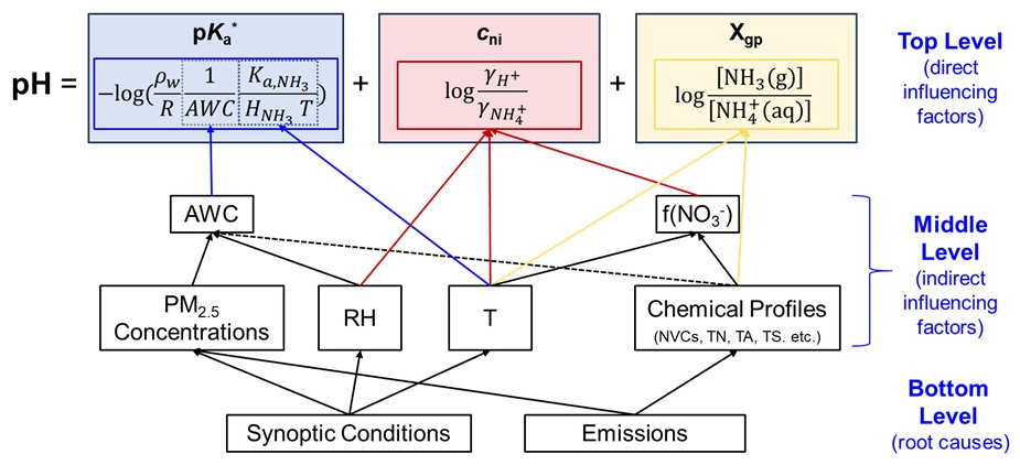
Figure 1 Hierarchical relationship among influencing factors of aerosol pH based on the multiphase buffer theory as established with the interpretive structural modeling approach.

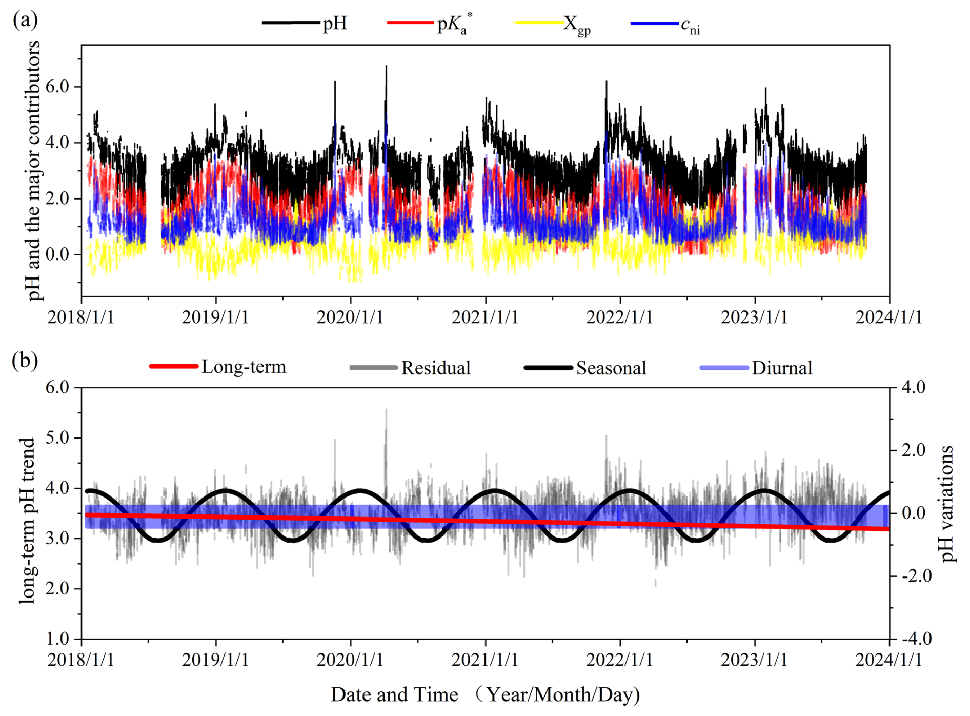
Figure 2 Major components of pH variations. (a) Decomposition into the $\mathrm{p}{K}_{\mathrm{a}}^{\ast }$, X_gp and c_ni based on the multiphase buffer theory. (b) Decomposition into long-term trends (left axis), seasonal variations, diurnal cycles and residuals (right axis) through time series analysis.

3.2 ISM coupled with time series analysis

With the above ISM approach, a quantitative analysis of each factor following the influencing lines can be achieved. In addition, when coupled with time series analysis, it can be applied to illustrate the driving factor of each time series component. Briefly, we can decompose each input parameter in ISORROPIA v2.3 into the four time series components (Sects. 2.1 and 2.2) and then apply each component to explain upper-level factors of corresponding component. For example, the seasonal variations in Y due to seasonal variations of factor x_i, ${\left.\frac{\partial Y}{\partial x_i}\right|}_{\text{seas}}$, is estimated as

$$\begin{array}{}\text{(3)}& {\left.{\displaystyle \frac{\partial Y}{\partial x_i}}\right|}_{\text{seas}}=f(\stackrel{\mathrm{‾}}{x_{\mathrm{1}}},\mathrm{\cdots },x_{i,\text{seas}}+\stackrel{\mathrm{‾}}{x_i},\mathrm{\cdots },\stackrel{\mathrm{‾}}{x_n})-f(\stackrel{\mathrm{‾}}{x_{\mathrm{1}}},\mathrm{\cdots },\stackrel{\mathrm{‾}}{x_n}),\end{array}$$

where x_i,seas is the decomposed seasonal variation in x_i. See more details in Sect. S2.

4 Driving factor analysis of long-term data in Changzhou

Here we applied the new framework (Sect. 3) to analyze the long-term data in Changzhou. From 2018 to 2023, around 90 % periods are within the ammonia-buffered regime, while the rest are due to low RH (<30 %) and aerosols not in a fully deliquescent state. Thus, the drivers of pH can be explained with the above framework.

The top-level ISM decomposition shows that the pH variations are mainly driven by the $\mathrm{p}{K}_{\mathrm{a}}^{\ast }$ (∼52 %) and c_ni (∼36 %), while the X_gp varies to a lesser extent (∼12 %, Figs. 2a and S2). In comparison, the time-series decomposition indicates that the pH variation is predominantly driven by seasonal variations and random residuals, while the long-term trend and diurnal cycle play minor roles on the variations (Fig. 2b). In the following we have analyzed the driving factors of each time series component.

4.1 Long-term trends

The long-term pH trends in Changzhou show a slight decreasing trend of $-\mathrm{0.05}{\mathrm{yr}}^{-\mathrm{1}}$ (Fig. 2b). The top-level ISM decomposition reveals that this is due to the competing trends of $\mathrm{p}{K}_{\mathrm{a}}^{\ast }$ and c_ni with X_gp: while $\mathrm{p}{K}_{\mathrm{a}}^{\ast }$ and c_ni decreased by −0.12 and $-\mathrm{0.14}{\mathrm{yr}}^{-\mathrm{1}}$, respectively, the X_gp increased by 0.21 yr⁻¹ (Fig. 3a).

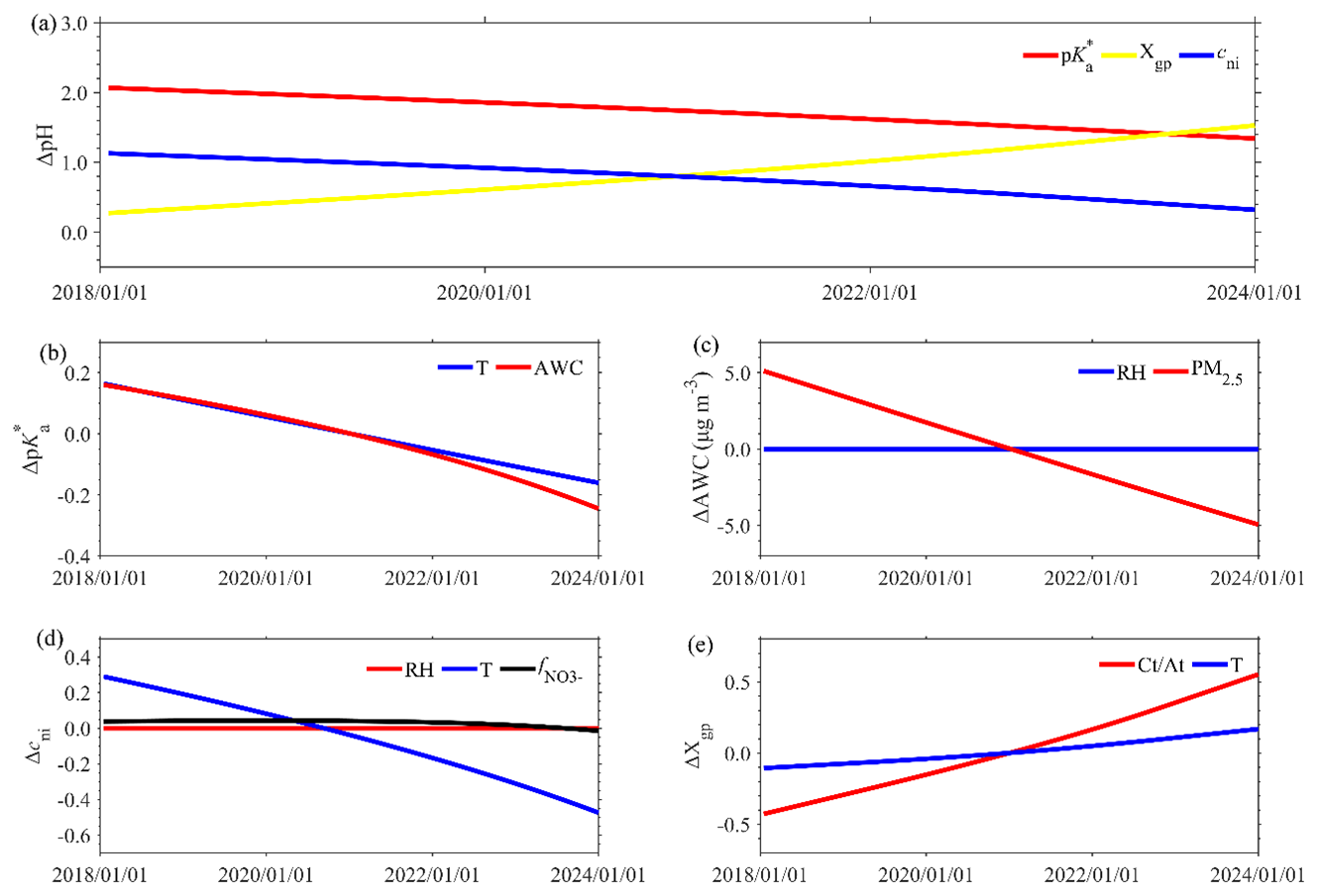
Figure 3 Influencing factors of long-term pH variation at different levels. (a) The first-level decomposition into $\mathrm{p}{K}_{\mathrm{a}}^{\ast }$, X_gp and c_ni. (b–e) Further investigation of the influencing factors of (b) $\mathrm{p}{K}_{\mathrm{a}}^{\ast }$ due to the T and AWC; (c) the AWC due to RH and PM_2.5; (d) c_ni due to RH, T and $f_{{\mathrm{NO}}_{\mathrm{3}}^{-}}$; and (e) X_gp due to $C_{\mathrm{t}}/A_{\mathrm{t}}$ and T.

A further delve into the middle-level factors in the ISM approach reveals that the $\mathrm{p}{K}_{\mathrm{a}}^{\ast }$ decrease is due to the combined effect of decreasing AWC and increasing temperature (Fig. 3b). The temperature increased by 0.74 K yr⁻¹ (Fig. S3), corresponding to a $\mathrm{p}{K}_{\mathrm{a}}^{\ast }$ of $-\mathrm{0.05}{\mathrm{yr}}^{-\mathrm{1}}$. In comparison, the AWC exhibited a decrease of $-\mathrm{1.57}\mathrm{\mu }\mathrm{g}{\mathrm{m}}^{-\mathrm{3}}{\mathrm{yr}}^{-\mathrm{1}}$ (Fig. S3), corresponding to a $\mathrm{p}{K}_{\mathrm{a}}^{\ast }$ of $-\mathrm{0.07}{\mathrm{yr}}^{-\mathrm{1}}$. The AWC decrease is primarily attributed to the PM_2.5 decrease (around $-\mathrm{1.6}\mathrm{\mu }\mathrm{g}{\mathrm{m}}^{-\mathrm{3}}{\mathrm{yr}}^{-\mathrm{1}}$), while the long-term RH shows minimal variation (Fig. 3c). As for c_ni, its decreasing trend is mainly attributed to increased temperature, corresponding to c_ni of $-\mathrm{0.13}{\mathrm{yr}}^{-\mathrm{1}}$ (Fig. 3d). RH and the fraction of ${\mathrm{NO}}_{\mathrm{3}}^{-}$ in particle-phase anions ($f_{{\mathrm{NO}}_{\mathrm{3}}^{-}}$) cause negligible effects on c_ni because they were nearly constant (Fig. S3). In terms of X_gp, its increase is due to the increase in both relative abundance of alkaline to acidic substances ($C_{\mathrm{t}}/A_{\mathrm{t}}$) and temperature (Fig. 3e), contributing to the X_gp increases of 0.16 and 0.05 yr⁻¹, respectively. Here the temperature influences X_gp through the gas–particle partitioning volatility of semi-volatile species like ammonium nitrate. The increase in $C_{\mathrm{t}}/A_{\mathrm{t}}$ is further due to a much larger decrease in A_t (sulfate, total nitrate, total chloride, etc.) than C_t (total ammonia and NVCs, etc.) (Fig. S3).

Overall, we see that the long-term pH trend shows only a slight decrease despite considerable emission changes during this period, which is a combined effect of decreased PM_2.5 while increased temperature and $C_{\mathrm{t}}/A_{\mathrm{t}}$.

4.2 Seasonal variations

Influencing factors of seasonal variation pH are analyzed in similar ways with the long-term trends (Fig. 4). Overall, the pH is higher in winter and spring than summer and autumn, with the amplitude of seasonal variations being 0.81 or the variation range being 1.62. The extent of variation is quantified by variation range hereinafter, which is the difference between the highest and lowest values for a given variable and for a given time series component. This cycle is consistent with $\mathrm{p}{K}_{\mathrm{a}}^{\ast }$ and c_ni, while it is in reverse phase with X_gp.

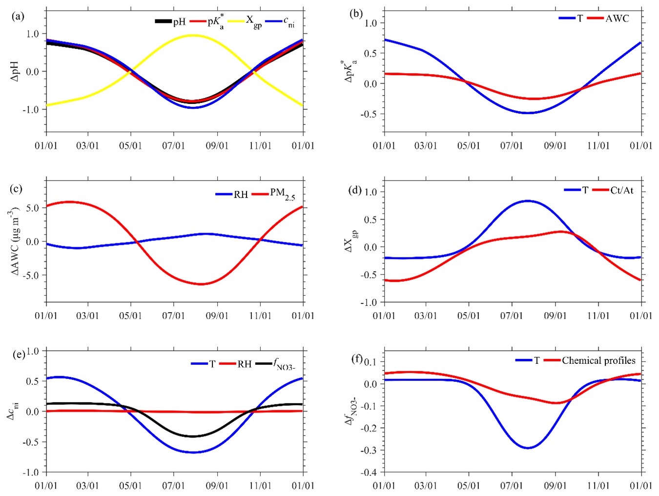
Figure 4 Influencing factors of the seasonal variations of aerosol pH. (a) The first-level decomposition into $\mathrm{p}{K}_{\mathrm{a}}^{\ast }$, X_gp and c_ni. (b–f) Further investigation of the influencing factors of (b) $\mathrm{p}{K}_{\mathrm{a}}^{\ast }$ due to the T and AWC, (c) the AWC due to RH and PM_2.5, (d) X_gp due to $C_{\mathrm{t}}/A_{\mathrm{t}}$ and T, (e) c_ni due to RH, T and $f_{{\mathrm{NO}}_{\mathrm{3}}^{-}}$, and (f) $f_{{\mathrm{NO}}_{\mathrm{3}}^{-}}$ due to T and chemical profiles.

The middle-level ISM decomposition demonstrates that the seasonal variation in $\mathrm{p}{K}_{\mathrm{a}}^{\ast }$ is mainly driven by the temperature (Fig. 4b). The variation in temperature is 23.26 K (Fig. S4), which corresponds to a $\mathrm{p}{K}_{\mathrm{a}}^{\ast }$ variation of 1.20. In comparison, the AWC varies to a lesser extent seasonally (Fig. S4), causing a relatively minor variation of 0.42 in $\mathrm{p}{K}_{\mathrm{a}}^{\ast }$. Seasonal variation in the AWC is further primarily attributed to the variation in PM_2.5 levels (approximately 25.4 µg m⁻³), as the seasonal RH varied little (Figs. 4c and S4). As for X_gp, its seasonal variation is influenced by both temperature and $C_{\mathrm{t}}/A_{\mathrm{t}}$, which correspond to variations in X_gp of −0.98 and −0.91, respectively (Fig. 4d). Higher temperature and $C_{\mathrm{t}}/A_{\mathrm{t}}$ during summer facilitate more NH_x remaining in the gas phase than winter (Fig. S4). Regarding c_ni, its seasonal variation is attributable to the combined effects of temperature and $f_{{\mathrm{NO}}_{\mathrm{3}}^{-}}$ (Fig. 4e), leading to variations in c_ni of 1.25 and 0.54, respectively. Again, the influence of RH is negligible due to its little variation (Fig. 4e). The seasonal variation of $f_{{\mathrm{NO}}_{\mathrm{3}}^{-}}$ is governed by significant variations of temperature (Fig. 4f). Temperature in winter is low enough and causes the vast majority of total nitrate to partition into the particle phase, leading to minor variation in $f_{{\mathrm{NO}}_{\mathrm{3}}^{-}}$ with temperature variations (Fig. S5). Conversely, higher temperatures in summer result in more total nitrate existing as HNO₃, and $f_{{\mathrm{NO}}_{\mathrm{3}}^{-}}$ is sensitive to temperature variations.

Overall, we see that the large seasonal variation in pH is mainly driven by the temperature as it plays a dominant role in $\mathrm{p}{K}_{\mathrm{a}}^{\ast }$, c_ni and X_gp (74 %, 89 % and 52 %, respectively). In comparison, the net influence of chemical profiles is relatively smaller, contributing 48 % and 10 % to X_gp and c_ni, respectively. That is, the seasonal variation in pH is largely driven by the meteorology (especially temperature) rather than emissions.

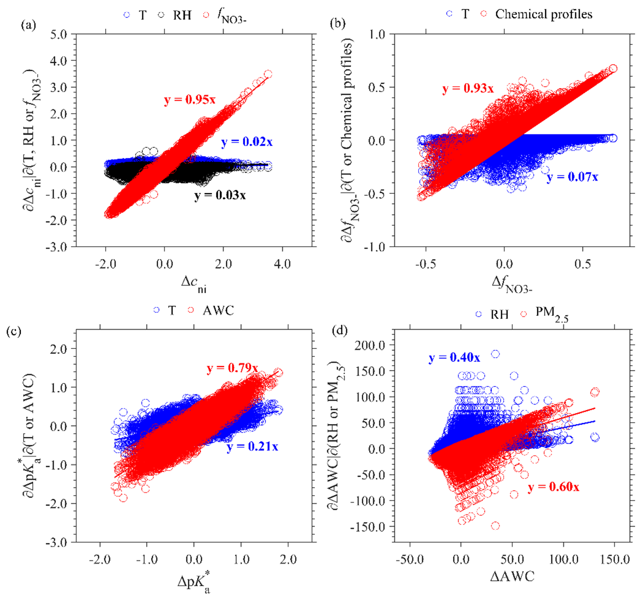
Figure 5 Influencing factors of the random residual of aerosol pH. (a) c_ni due to T, RH and $f_{{\mathrm{NO}}_{\mathrm{3}}^{-}}$; (b) $f_{{\mathrm{NO}}_{\mathrm{3}}^{-}}$ due to T and chemical profiles; (c) $\mathrm{p}{K}_{\mathrm{a}}^{\ast }$ due to the T and AWC; and (d) the AWC due to RH and PM_2.5.

4.3 Diurnal cycles

Diurnal cycles of pH are higher at nighttime than daytime, with a variation range of 0.65. Similar to the seasonal variations, the diurnal cycle is also consistent with $\mathrm{p}{K}_{\mathrm{a}}^{\ast }$ and c_ni trend, while it is in a reverse trend with X_gp (Fig. S6a), with their contribution to pH being 0.70, 0.58 and −0.63, respectively.

The major driving factor of diurnal cycles in $\mathrm{p}{K}_{\mathrm{a}}^{\ast }$ is different to that of seasonal variations. First, the diurnal cycle of $\mathrm{p}{K}_{\mathrm{a}}^{\ast }$ is driven by both the AWC (0.45) and temperature (0.25) (Fig. S6b), in contrast to the dominance of temperature in seasonal variations (Sect. 4.2). This is mainly due to the much smaller temperature variation range diurnally (4.87 K; Fig. S7) than seasonally (23.26 K). In addition, diurnal variation in the AWC is primarily influenced by RH (Fig. S6c) due to the larger RH diurnal variations (16 % versus 3 % in seasonal variations; Figs. S7 and S4), in contrast with the PM_2.5 dominance in seasonal variations. In terms of X_gp, its dominant driving factor of diurnal cycles is $C_{\mathrm{t}}/A_{\mathrm{t}}$, in contrast with the dominance of temperature in seasonal variations (Fig. S6d). Diurnal cycles of c_ni are due to the combined effects of temperature and $f_{{\mathrm{NO}}_{\mathrm{3}}^{-}}$ (Fig. S6e), where $f_{{\mathrm{NO}}_{\mathrm{3}}^{-}}$ is further mainly driven by chemical profiles (Fig. S6f).

4.4 Residual

The random residual of aerosol pH is another major contributor to pH temporal variations, which is comparable with the seasonal variations. Distinct from all the three components above, the largest top-level contributor to random residuals turns out to be c_ni (82 %), even exceeding that of $\mathrm{p}{K}_{\mathrm{a}}^{\ast }$ (42 %), while X_gp causes a net negative effect (−24 %; Fig. S8). Moreover, random fluctuations in c_ni are almost entirely due to variations in $f_{{\mathrm{NO}}_{\mathrm{3}}^{-}}$ (∼95 %; Fig. 5a), which are primarily driven by chemical profiles (∼93 %; Fig. 5b). The $\mathrm{p}{K}_{\mathrm{a}}^{\ast }$ random fluctuations are mainly caused by the AWC (∼79 %), which is further attributed mainly (∼60 %) to PM_2.5 variations (Fig. 5c and d). Random variations of X_gp are dominated by the chemical profiles, similar to diurnal cycles and long-term trend (Fig. S9). Overall, PM_2.5 and chemical profiles are the major influencing factors for the random residual of pH, underscoring the prominence of emissions over meteorology.

5 Overall contributions and implications

Figure 6 shows the distinct major influencing factors of aerosol pH in the four time series components, where the factors contributing less than $\left|\mathrm{10}\mathit{\%}\right|$ are not shown. Overall, $\mathrm{p}{K}_{\mathrm{a}}^{\ast }$ is the dominant influencing factor of pH variations, being the major contributor in all components and playing a pivotal role in seasonal and diurnal cycles (Fig. 6). c_ni is another dominant factor for pH variations, especially in random fluctuations. X_gp shows a reverse trend with pH in all components. As seasonal and random variations largely regulate the pH temporal variations, $\mathrm{p}{K}_{\mathrm{a}}^{\ast }$ and c_ni contribute more to pH than X_gp.

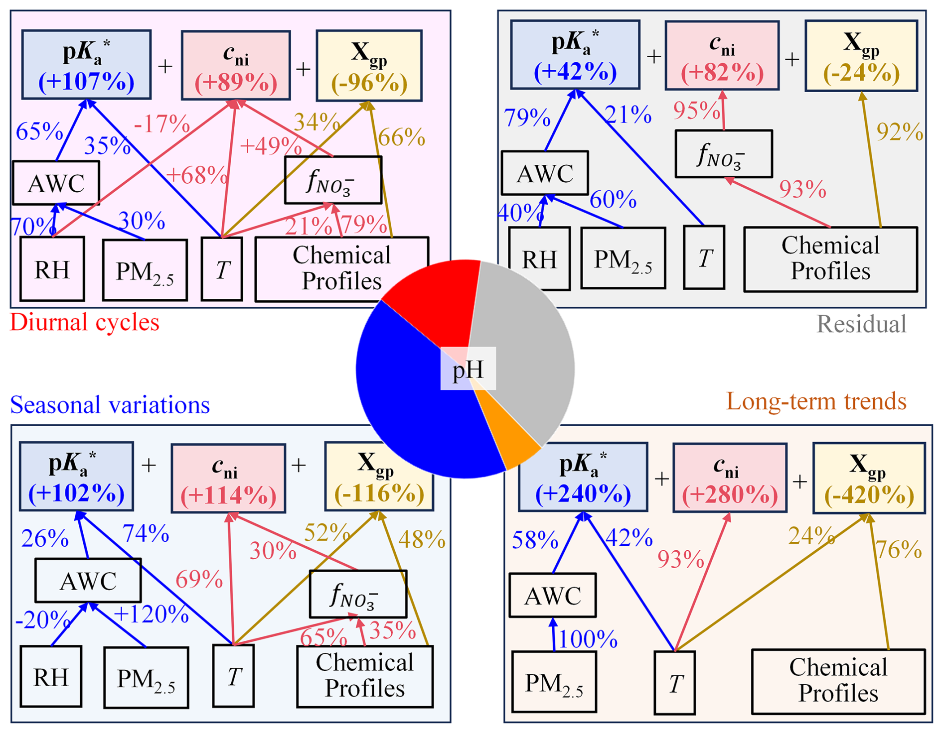
Figure 6 Hierarchical relationship among major influencing factors of aerosol pH variations for the 4 time series components, respectively. Here, the percentage variations are derived by the variations due to factor X to overall variations. For example, the contribution of $\mathrm{p}{K}_{\mathrm{a}}^{\ast }$ variations to seasonal variations of pH is derived by $\frac{\mathrm{\Delta }\mathrm{p}{K}_{\mathrm{a},\text{seas}}^{\ast }}{\mathrm{\Delta }{\text{pH}}_{\text{seas}}}\times \mathrm{100}\mathit{\%}$, where the overall pH variations $\mathrm{\Delta }{\text{pH}}_{\text{seas}}=\mathrm{\Delta }\mathrm{p}{K}_{\mathrm{a},\text{seas}}^{\ast }+\mathrm{\Delta }{c}_{\text{ni},\text{seas}}+\mathrm{\Delta }{X}_{\text{gp},\text{seas}}$. Factors contributing less than $\left|\mathrm{10}\mathit{\%}\right|$ are not shown.

Deeper-level driver analysis show that meteorology plays a more important role than chemical profiles in explaining the pH temporal variations (57 % versus 22 %; Fig. S10). Temperature is the major contributor, which explains seasonal variations in $\mathrm{p}{K}_{\mathrm{a}}^{\ast }$, c_ni and X_gp of 74 %, 89 % and 52 %, respectively, and it is also important in diurnal cycles and long-term trends. RH plays an important role in diurnal cycles, accounting for 70 % of the AWC diurnal variations and thus indirectly exerting an important effect on $\mathrm{p}{K}_{\mathrm{a}}^{\ast }$ (∼46 %). In comparison, chemical profiles are essential for explaining long-term trends in X_gp, and they also provide a pivotal role in random fluctuations and diurnal cycles for c_ni. The PM_2.5 concentration is an overall effect of meteorology and emissions. PM_2.5 is the dominant contributor to the AWC in all components except diurnal cycles, exerting an indirect influence on $\mathrm{p}{K}_{\mathrm{a}}^{\ast }$. Overall, temperature is critical in explaining pH variations (48 %; Fig. S10), followed by chemical profiles, PM_2.5 concentrations and RH (22 %, 21 % and 9 %, respectively).

The quantitative framework we proposed here can provide a clear understanding of the drivers of aerosol acidity temporal variations, with information on both quantitative contributions and the underlying mechanisms. Our findings suggest that the relative importance of synoptic conditions versus emissions in aerosol acidity variations differed much with the timescale of concern and are is due to different major mechanisms. In Changzhou, synoptic conditions are more important for seasonal variations and diurnal cycles of pH, while emissions cause a greater effect on pH random fluctuations. For the long-term trends, both emissions and synoptic conditions are important. These findings generally agree with previous studies in the YRD region. For example, two previous studies on aerosol acidity in Shanghai (Lv et al., 2024; Zhou et al., 2022) also found that synoptic conditions played important role in seasonal and diurnal variations of aerosol pH, while for long-term pH trends, the primary drivers were attributed to emissions in acidic anions and NVCs. Regardless, our analysis here provided more systematic insight and theoretically explanations into the underlying mechanisms of each influencing factor compared with previous studies. In other places, this framework still applies, while the conclusions may vary. This quantitative understanding of the driving factors of aerosol acidity is important in acidity-relevant process studies and policy-making, such as nitrate control (Guo et al., 2017), sulfate formation (Cheng et al., 2016; Zheng et al., 2024a) and nitrogen depositions (Nenes et al., 2021).