Microphysics regimes due to haze–cloud interactions: cloud oscillation and cloud collapse

It is known that aqueous haze particles can be activated into cloud droplets in a supersaturated environment. However, haze–cloud interactions have not been fully explored, partly because haze particles are not represented in most cloud-resolving models. Here, we conduct a series of large-eddy simulations (LESs) of a cloud in a convection chamber using a haze-capable Eulerian-based bin microphysics scheme to explore haze–cloud interactions over a wide range of aerosol injection rates. Results show that the cloud is in a slow microphysics regime at low aerosol injection rates, where the cloud responds slowly to an environmental change and droplet deactivation is negligible. The cloud is in a fast microphysics regime at moderate aerosol injection rates, where the cloud responds quickly to an environmental change and haze–cloud interactions are important. More interestingly, two more microphysics regimes are observed at high aerosol injection rates due to haze–cloud interactions. Cloud oscillation is driven by the oscillation of the mean supersaturation around the critical supersaturation of aerosol due to haze–cloud interactions. Cloud collapse happens under weaker forcing of supersaturation where the chamber transfers cloud droplets to haze particles efficiently, leading to a significant decrease (collapse) in cloud droplet number concentration. One special case of cloud collapse is the haze-only regime. It occurs at extremely high aerosol injection rates, where droplet activation is inhibited, and the sedimentation of haze particles is balanced by the aerosol injection rate. Our results suggest that haze particles and their interactions with cloud droplets should be considered, especially in polluted conditions.

1 Introduction

Atmospheric clouds play an important role in Earth's radiation balance and hydrological cycle. Their optical properties and precipitation efficiency are strongly influenced by cloud microphysical composition (e.g., droplet size and concentration) and processes (e.g., droplet formation and growth). It is known that cloud droplets in the atmosphere grow from aerosol particles, most of which contain water-soluble materials, such as sodium chloride or ammonium sulfate. These water-soluble aerosol particles first absorb water vapor in a subsaturated environment to become aqueous droplets (known as haze particles) through deliquescence. Haze particles can then be activated into cloud droplets in a sufficiently supersaturated environment (i.e., when relative humidity is higher than 100 %). The supersaturation needed to activate cloud droplets depends on aerosol properties as explained by Köhler theory (Twomey, 1959). Changes in aerosol properties from various anthropogenic and natural emissions can have a significant impact on clouds, thereby affecting the climate system substantially. So far, aerosol–cloud interaction remains one of the largest uncertainties in climate projection, partly because of the poor representation of cloud microphysical processes in models and incomplete understanding of those processes at the fundamental level (Morrison et al., 2020).

It is challenging to isolate the impact of aerosol on cloud properties and evolution in the real atmosphere because cloud microphysics, dynamics, and thermodynamics are coupled in a complex way. In addition, cloud properties fluctuate over time and space, making them difficult to thoroughly sample and interpret. In contrast, the Michigan Tech convection cloud chamber, also known as the Pi chamber, can maintain a steady-state cloud for several hours under well-controlled initial and boundary conditions (Chang et al., 2016). The Pi chamber produces a well-mixed supersaturated environment by maintaining a warm, humid bottom surface and a cool, humid top surface through Rayleigh–Bénard convection. The cloud is formed by continuously injecting aerosol particles into the supersaturated environment, and it can reach a steady state when the droplet activation rate is balanced by the droplet sedimentation rate. Cloud properties are controlled by aerosol properties (e.g., aerosol size, chemical composition, and injection rate) and boundary conditions (e.g., top and bottom temperatures – the driving factor to create a supersaturated environment). Steady-state cloud properties in the Pi chamber can be measured in great detail, which provides a unique opportunity to explore aerosol–cloud–turbulence interactions in well-controlled environments.

Previous Pi chamber experiments have shown that increasing aerosol injection rates result in higher cloud droplet number concentrations, smaller mean droplet radii, and narrower droplet size distributions (Chandrakar et al., 2016). These trends are consistent with results from cloud-resolving large-eddy simulations (LESs) of the Pi chamber (Thomas et al., 2019). Krueger (2020) derived an analytical expression for the equilibrium cloud droplet size distribution in a turbulent cloud chamber with the assumption of uniform supersaturation. This analytic droplet size distribution, along with three others that account for supersaturation fluctuations in different ways, has been compared with measured droplet size distributions in the Pi chamber (Chandrakar et al., 2020). Results show that all four analytical droplet size distributions match the observed distribution reasonably well for monodisperse aerosol injection. However, none of them matched well for polydisperse aerosol injections. Chandrakar et al. (2020) argued that it might be due to the Ostwald ripening effect (Korolev, 1995; Jensen and Nugent, 2017; Yang et al., 2018), which is not considered in those analytical models. Recently, Shaw et al. (2023) developed a theoretical model to describe the microphysical state of well-mixed monodisperse droplets in cloudy Rayleigh–Bénard convection. The model predicts that N_d∼n_in and q_l∼n_in in the slow microphysics regime (i.e., at low aerosol injection rates), while $N_{\mathrm{d}}\sim n_{\mathrm{in}}^{\mathrm{5}/\mathrm{3}}$ and $q_{\mathrm{l}}\sim n_{\mathrm{in}}^{\mathrm{2}/\mathrm{3}}$ in the fast microphysics regime (i.e., at high aerosol injection rates), where N_d is the droplet number concentration, n_in the aerosol injection rate, and q_l the liquid water mixing ratio. The slow microphysics regime refers to a relatively clean condition where the cloud would respond slowly to an environmental change, while the fast microphysics regime refers to a relatively polluted condition where the cloud would respond quickly to an environmental change. Pi chamber observations confirm the nonlinear relationship between q_l and n_in in the fast microphysics regime (see Fig. 7 in Shaw et al., 2023), but more investigations are needed to evaluate the theory and its ability to represent microphysical properties in a convection cloud chamber.

Besides cloud droplets, observations using a digital optical particle counter show the existence of haze particles with diameters down to 0.6 µm (detection limit) in the Pi chamber (Prabhakaran et al., 2020). Results from direct numerical simulations with Lagrangian aerosol/droplet microphysics show that haze particles undergo multiple activation and deactivation cycles in a convection chamber (MacMillan et al., 2022). However, previous theoretical studies do not include the haze activation process for simplification (Krueger, 2020; Chandrakar et al., 2020; Shaw et al., 2023). In addition, most previous Pi chamber simulations do not fully resolve haze particles because in these simulations as well as in most atmospheric cloud simulations, droplets are formed directly from aerosol particles based on Twomey-type activation parameterizations (Twomey, 1959), in which aerosols are activated into cloud droplets if the environmental supersaturation is larger than the aerosol's critical supersaturation (Thomas et al., 2019; Grabowski, 2020). Recently, Yang et al. (2023) developed a haze-capable bin microphysics scheme to simulate the Pi chamber by directly calculating the condensational growth of haze and cloud droplets, which naturally resolves droplet activation process without further parameterization. Simulations using this haze-capable bin scheme can capture haze droplet size distributions, aligning well with simulations from a Lagrangian microphysics scheme, with the latter serving as the “truth” because it does not suffer numerical diffusion during droplet growth and advection (Morrison et al., 2018; Grabowski et al., 2019). Results also show that the simulated cloud properties using the haze-capable bin microphysics scheme agree reasonably well with those using Twomey-type activation. We refer to the Twomey-type activation scheme as the cloud condensation nuclei (CCN)-based bin microphysics scheme because it treats dry aerosols as CCN which behave like cloud droplets immediately after the environmental supersaturation is larger than a critical supersaturation (i.e., without resolving the growth of haze particles). Good agreement between the haze-capable and CCN-based bin microphysics schemes suggests that if we are only interested in the cloud microphysical properties, we could still use Twomey-type activation parameterizations. However, only two aerosol injection rates were used in Yang et al. (2023), and thus, it is not clear whether results from the CCN-based bin microphysics scheme will always be similar to those from the haze-capable bin microphysics scheme, especially in a low-supersaturation environment where haze–cloud interaction is important (e.g., Prabhakaran et al., 2020).

In this study, we conduct a series of large-eddy simulations of the Pi chamber using both CCN-based and haze-capable bin microphysics schemes over a wide range of aerosol injection rates. We aim to address the following questions:

• (a)

  How do cloud microphysical properties change over a wide range of aerosol injection rates (for constant boundary conditions)?

• (b)

  Do simulation results agree with previous theoretical studies?

• (c)

  How important are haze–cloud interactions in the Pi chamber as well as in natural clouds?

Specifically, related to question (a), we aim to explore how the steady-state supersaturation, the mean droplet radius, N_d, and q_l change with aerosol injection rate. For question (b), we aim to evaluate steady-state droplet size distribution predicted in Krueger (2020) and Chandrakar et al. (2020), as well as slow and fast microphysics regimes predicted in Shaw et al. (2023). Related to question (c), we aim to know whether cloud properties simulated by the CCN-based bin microphysics scheme are always consistent with those from the haze-capable bin microphysics scheme, as indicated by Yang et al. (2023), or if haze-capable microphysics must be used for certain atmospheric conditions. Note that the Pi chamber could be connected to some simple cloud systems like fog or non-drizzling shallow-layer clouds. Therefore, what we learn about haze–cloud interactions can be transferred. We want to understand the conditions under which haze–cloud interactions become important, connecting our work to a broader atmospheric science context.

2 Model description and setup

We employ SAM-Chamber to conduct large-eddy simulations of the Pi chamber in this study. SAM-Chamber is an adapted and modified version of the System for Atmospheric Modeling (SAM; Khairoutdinov and Randall, 2003) with the major changes in the consideration of four side walls and the top surface to represent the chamber boundary condition (detailed in Thomas et al., 2019). SAM-Chamber has been used to simulate the Pi chamber to explore several topics, including the impact of various bin microphysics and advection schemes on Pi chamber simulations (Yang et al., 2022), impact of supersaturation fluctuations on droplet formation and growth (Prabhakaran et al., 2022; Anderson et al., 2023), development of a haze-capable microphysics scheme (Yang et al., 2023), investigation of drizzle initiation in larger convection chambers (Thomas et al., 2023; Wang et al., 2024c), glaciation of mixed-phase clouds (Wang et al., 2024a), and dual signatures of entrainment (Wang et al., 2024b). SAM-Chamber employed in this study is the one used in Wang et al. (2024c), where the wall fluxes of momentum, sensible heat, and moisture are modeled in accordance with Monin–Obukhov similarity theory (MOST; Monin and Obukhov, 1954) as before but with the following changes: (1) the roughness lengths for momentum (z₀), sensible heat (z_t), and moisture (z_q) are tuned to match the mean fluxes obtained in the direct numerical simulations. (2) The hydrostatic stability on the side walls is assumed to be neutral, as the buoyancy is parallel rather than normal to the side walls. More details on the wall modeling are addressed in Wang et al. (2024c; see Sect. 2 and Appendix B therein).

(based on Wang et al., 2024c)(Yang et al., 2023)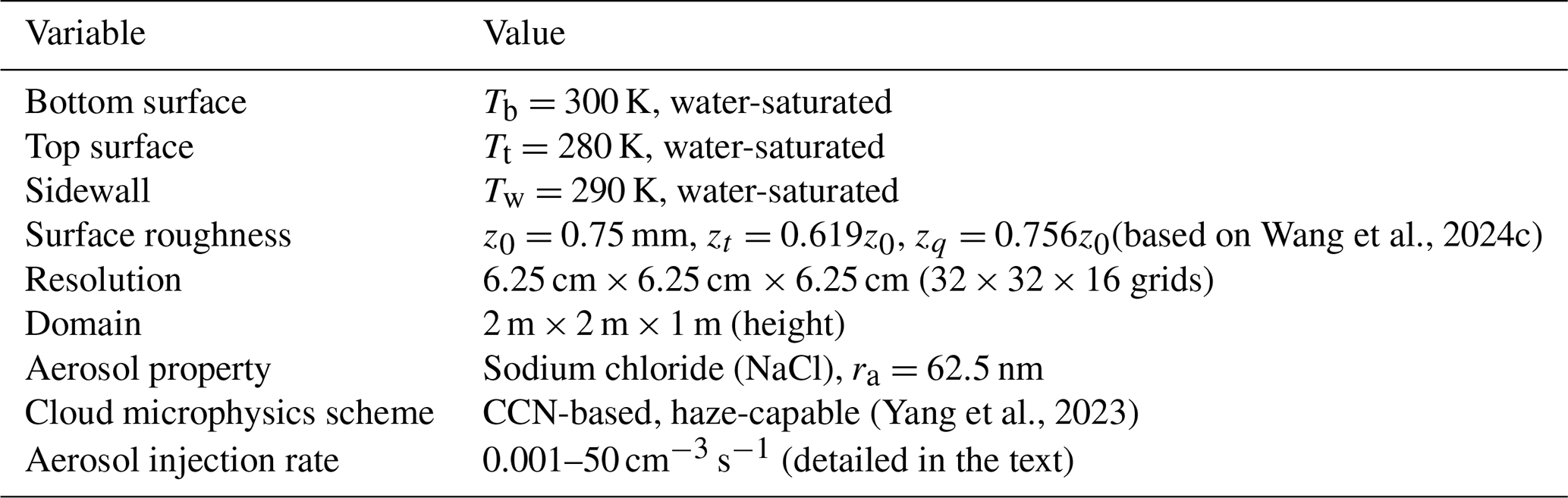

Table 1 Summary of model setup.

The model setup is summarized in Table 1. The temperature of the bottom surface is set to be 300 K, the top surface to be 280 K, and the side walls to be 290 K. In previous SAM-Chamber simulations (Thomas et al., 2019; Yang et al., 2022, 2023), the side walls were set to be subsaturated such that the domain-averaged supersaturation without cloud is about 2.5 % based on early chamber observations (Chandrakar et al., 2016). Subsaturated side walls serve as a sink for water vapor, tending to evaporate droplets nearby. Sidewalls have been improved (i.e., closer to be water saturated) recently in the real Pi chamber, such that clouds can form at much smaller top and bottom temperature differences (Prabhakaran et al., 2020). In this study, all surfaces are set to be saturated with respect to water. The impact of side wall conditions on cloud properties will be discussed later. The simulation domain is 2 m × 2 m × 1 m with 6.25 cm grid spacing in all three directions. This grid spacing falls in the inertial subrange, according to the direct numerical simulations with similar Reynolds number and Rayleigh number performed by Wang et al. (2024d).

To mimic continuous injection of salt particles, monodisperse sodium chloride aerosol particles with a dry radius of 62.5 nm are added in each grid box after each time step, as in previous studies (Yang et al., 2022, 2023). Cloud droplet formation and growth by condensation are simulated using either a CCN-based or haze-capable bin microphysics scheme. Both schemes are two-moment bin microphysics schemes based on Chen and Lamb (1994), with some differences detailed in Yang et al. (2023) and summarized below. For the CCN-based bin microphysics scheme (referred to as the CL_CCN), droplet size distribution is represented by 33 mass-doubling bins starting from 1 µm radius. Dry aerosol particles stay in the aerosol category, and they will be moved to the first bin of the cloud category if the environmental supersaturation (in their grid box) is larger than the critical supersaturation of the aerosol (0.08 % for a salt particle of 62.5 nm in radius). Solute and curvature effects are not considered for droplet growth by condensation. Note that such treatment of cloud microphysical processes – Twomey-type parameterization of droplet formation and neglect of solute and curvature effects on droplet growth – is quite common in atmospheric cloud simulations. For the haze-capable bin microphysics scheme (referred to as the CL_Haze), aqueous droplets (including haze and cloud) are represented by 40 mass-doubling bins starting from 0.1 µm radius. Dry aerosol particles initially become haze with the equilibrium size at a relative humidity of 90 % (same as in Yang et al., 2023). The growth of haze and cloud droplets via condensation is calculated explicitly with solute and curvature effects considered, and thus the activation process from haze particle to cloud droplet is naturally resolved. Following Yang et al. (2023), haze particles here refer to droplets with radii smaller than 1 µm, which is the bin edge closest to the critical radius of the aerosol (0.92 µm). In this study, we consider the solute and curvature effects for the growth of cloud droplets (radii larger than 1 µm) in both CL_CCN and CL_Haze schemes. The main difference between the CL_CCN scheme and the CL_Haze scheme is the way to handle droplet activation as detailed above. Although all chamber surfaces are saturated with respect to water, droplet deactivation by evaporation can still occur due to turbulent supersaturation fluctuations. For the CL_CCN scheme, evaporated droplets will be moved to the aerosol category if their radii get smaller than 1 µm in radius (the deactivation process). For the CL_Haze scheme, deactivated droplets remain as haze particles. Efflorescence is not considered, and if haze particles are less than 0.1 µm in radius, they stay in the smallest droplet bin. In both schemes, droplets can only be lost through the bottom surface due to sedimentation but not through the side walls.

Following the modeling studies by Yang et al. (2023) and Wang et al. (2024a, c, b), sodium chloride aerosol particles of a 62.5 nm radius are injected uniformly throughout the computational domain at a prescribed volumetric rate. A total of 25 aerosol injection rates (n_in) are employed to explore their impact on cloud properties. n_in ranges from 0.001 to 50 cm⁻³ s⁻¹ in the following way: 0.001 to 0.005 cm⁻³ s⁻¹ every 0.001 cm⁻³ s⁻¹, 0.01 to 0.05 cm⁻³ s⁻¹ every 0.01 cm⁻³ s⁻¹, 0.1 to 0.5 cm⁻³ s⁻¹ every 0.1 cm⁻³ s⁻¹, 1.0 to 5.0 cm⁻³ s⁻¹ every 1.0 cm⁻³ s⁻¹, and 10.0 to 50.0 cm⁻³ s⁻¹ every 10.0 cm⁻³ s⁻¹. Note that 14 values of n_in between 0.2 and 13 cm⁻³ s⁻¹ were used in recent Pi chamber experiments (see Fig. 7 in Shaw et al., 2023), while only two values (0.25 and 2.5 cm⁻³ s⁻¹) were used in the Pi chamber simulations by Yang et al. (2023). Here, we cover a range of n_in that can be achieved in the Pi chamber, while extending n_in to represent extremely clean and polluted conditions. Although these exceptionally small and large n_in values might be difficult to achieve in the real chamber mainly due to the current limitations of aerosol injection, they are helpful to explore haze–cloud interactions in various microphysics regimes that will be discussed in the next section.

The time step is 0.02 s, and the total simulation is 1 h. The domain-averaged data are output every minute from the beginning of the simulation, while instantaneous 3-D data are output every 5 min in the second half of the simulation.

3 Results

3.1 Impact of aerosol injection rate on bulk cloud properties

Figure 1 shows the impact of n_in on droplet mean radius (r_d), N_d, and q_l. Here, q_l is the liquid water mixing ratio. Specifically, r_d and N_d are calculated only for cloud droplets whose radii are larger than 1 µm. $q_{\mathrm{l}}=q_{\mathrm{c}}+q_{\mathrm{h}}$ for the CL_Haze scheme, where q_c is the cloud water mixing ratio (for droplets radii larger than 1 µm) and q_h is the haze water mixing ratio (for droplets radii smaller than 1 µm), while q_l=q_c for the CL_CCN scheme. Each dot in the figure represents a temporally averaged (over the second half an hour) and spatially averaged (over the whole domain) value for one aerosol injection rate when using either the CL_CCN (black) or CL_Haze (red) scheme. Results show that cloud microphysical properties based on these two schemes are similar, suggesting that using the Twomey-type activation parameterization is good enough to simulate bulk cloud properties, especially for N_d and q_l.

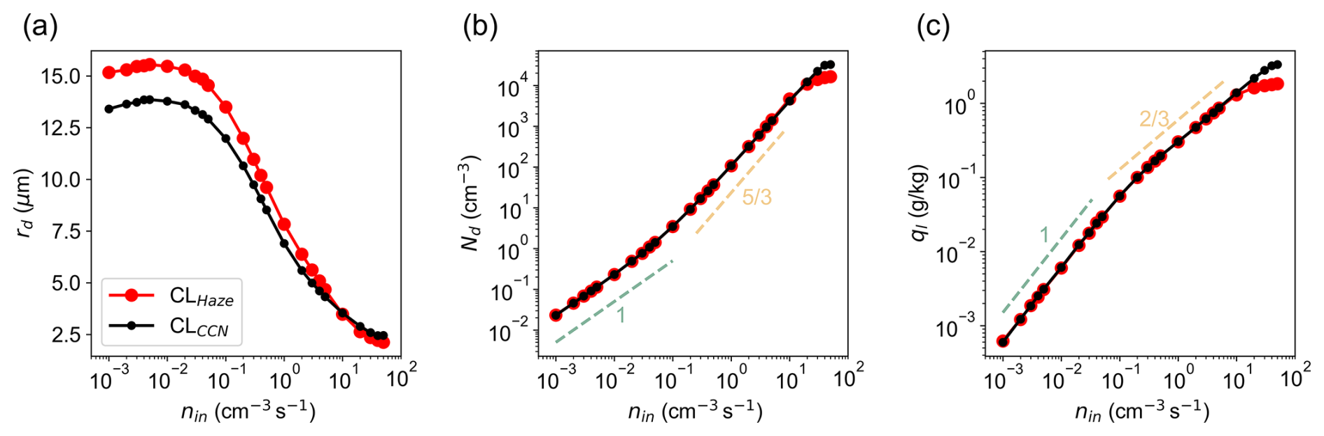
Figure 1 Spatially averaged (over the whole domain) and temporally averaged (in the second half an hour) (a) mean droplet radius r_d, (b) droplet number concentration N_d, and (c) liquid water mixing ratio q_l at various aerosol injection rates. Black and red dots are results using CL_CCN and CL_Haze schemes, respectively. Each dot represents the average of the variable over the whole domain from the second half an hour. The light-green and yellow-colored dashed lines in (b) and (c) are scaling relationships based on Shaw et al. (2023) in slow and fast microphysics regimes, respectively. Note that we only consider cloud droplets whose radii are larger than 1 µm to calculate r_d and N_d here.

The steady-state droplet size distributions based on the CL_CCN and CL_Haze schemes are shown in Fig. 2a–b. The distribution becomes narrower and shifts to smaller sizes with n_in, consistent with previous Pi chamber observations (Chandrakar et al., 2016) and simulations (Thomas et al., 2019; Yang et al., 2023). The mode of small haze particles can only be captured by the CL_Haze scheme and is enhanced as n_in increases (Fig. 2b). We also compare the simulated size distributions with four analytical droplet size distributions: arexp (−br⁴) (Fig. 2c), arexp (−br²) (Fig. 2d), ar²exp (−br³) (Fig. 2e), and $a\sqrt{r}\exp (-b{r}^{\mathrm{3}})$ (Fig. 2f), where a and b represent the combinations of other variables and parameters except for r. All these analytical distributions use steady-state N_d and q_c from the SAM-Chamber simulations as input to calculate the parameters a and b. The precise formulas are displayed in Fig. 2c–f. Chandrakar et al. (2020) detailed the assumptions regarding these analytical distributions and evaluated them with the Pi chamber observations. In short, arexp (−br⁴) is derived from the assumption of droplet growth in a constant supersaturation environment with size-dependent removal (Krueger, 2020), arexp (−br²) comes from droplet growth in a fluctuating supersaturation environment with size-independent removal (McGraw and Liu, 2006; Saito et al., 2019), ar²exp (−br³) results from the principle of maximum entropy assumption (Liu and Hallett, 1998), and $a\sqrt{r}\exp (-b{r}^{\mathrm{3}})$ comes from droplet growth in a fluctuating supersaturation environment with size-dependent removal (Chandrakar et al., 2020). Results show that the simulated cloud droplet size distributions are closer to arexp (−br⁴), ar²exp (−br³), and $a\sqrt{r}\exp (-b{r}^{\mathrm{3}})$, compared to arexp (−br²), which produces significantly broader spectra (Fig. 2d). Furthermore, the haze mode is not captured by any analytical distribution, simply because none of those analytical models considers the full activation process – from haze particles to cloud droplets.

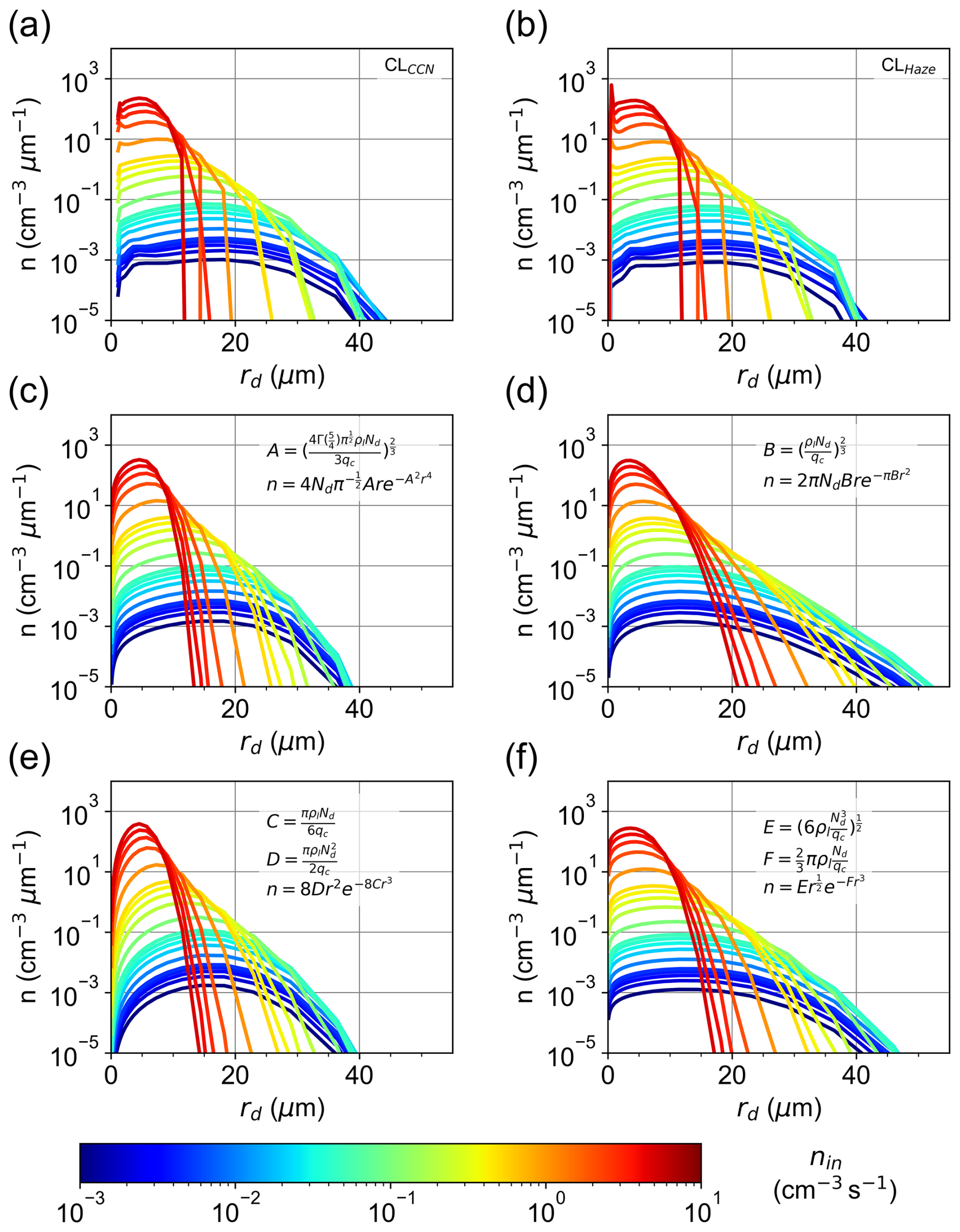
Figure 2 Steady-state droplet size distributions for different aerosol injection rates when using (a) CL_CCN and (b) CL_Haze schemes. (c–f) Four analytical droplet size distributions using the domain-averaged N_d and q_c as input, with the precise formulas displayed in the legend.

Slow and fast microphysics regimes are observed as shown in Fig. 1. The impact of n_in on the mean supersaturation s and its standard deviation σ_s (see Fig. 3) indicates the physical origin of these two microphysics regimes and its connection to various activation regimes. The slow microphysics regime is observed when n_in< 0.1 cm⁻³ s⁻¹. In this regime, few droplets (i.e., very small N_d shown in Fig. 1b) grow in a high-supersaturation environment (Fig. 3a) before they fall out, leading to a roughly constant r_d (Fig. 1a) and a linear relationship between n_in and N_d (Fig. 1b) as well as q_l (Fig. 1c) as predicted by Shaw et al. (2023). Based on the definition in Prabhakaran et al. (2020), the cloud is in the mean-supersaturation-dominated activation regime where s>>s_crit.

When 0.1 cm⁻³ s⁻¹ $<n_{\mathrm{in}}<\mathrm{10.0}$ cm⁻³ s⁻¹, the cloud is in the fast microphysics regime, in which more cloud droplets compete with each other for available water vapor needed for their condensational growth, leading to larger N_d and smaller r_d. In this regime, r_d, s, and σ_s decrease with n_in, while $N_{\mathrm{d}}\sim n_{\mathrm{in}}^{\mathrm{5}/\mathrm{3}}$ and $q_{\mathrm{l}}\sim n_{\mathrm{in}}^{\mathrm{2}/\mathrm{3}}$, consistent with theory. Based on the definition in Prabhakaran et al. (2020), the cloud is in the supersaturation-fluctuation-influenced activation regime (s>s_crit and σ_s>s_crit) or supersaturation-fluctuation-dominated activation regime (s<s_crit and σ_s>s_crit), but the latter is barely observed in our results.

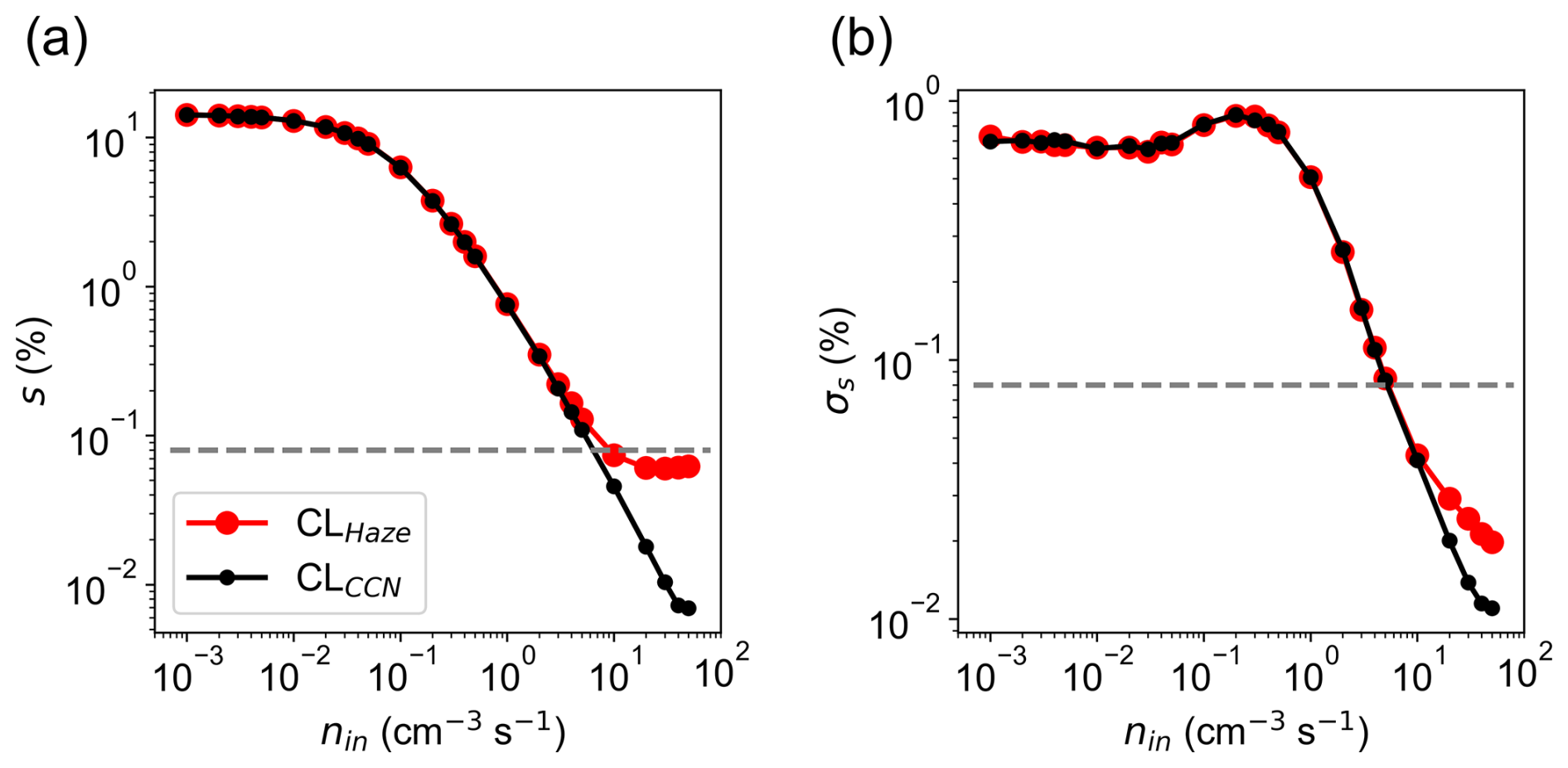
Figure 3 Spatially averaged (over the whole domain) and temporally averaged (in the second half an hour) (a) mean supersaturation s and (b) standard deviation of supersaturation σ_s at various aerosol injection rates. Black and red dots are results using CL_CCN and CL_Haze schemes, respectively. Each dot represents the average of the variable over the whole domain from the second half an hour. The horizontal dashed line indicates the critical supersaturation of injected aerosols (0.08 %).

The scaling laws for N_d and q_l do not work well for n_in≥10.0 cm⁻³ s⁻¹ when using the CL_Haze scheme (Fig. 1b and c). Also note that both s and σ_s are smaller than s_crit at these high aerosol injection rates, suggesting that droplet activation is strongly suppressed. It is interesting to see that s approaches a value that is slightly smaller than s_crit when using the CL_Haze scheme, while in contrast, s continuously decreases with n_in and approaches 0 when using the CL_CCN scheme. This is because the cloud system is buffered by a huge number of cloud droplets in the polluted condition and s should be close to the equilibrium supersaturation over droplets (which is s_crit when using the CL_Haze scheme where solute and curvature effects are considered or 0 when using the CL_CCN scheme). This regime turns out to be very important for haze–cloud interactions, which will be explored in the following section.

Table 2 Spatially and temporally averaged aerosol/haze number concentration (N_a or N_h; cm⁻³), cloud droplet number concentration (N_d; cm⁻³), mean cloud droplet radius (r_d; µm), droplet activation rate (R_act; cm⁻³ s⁻¹), and droplet deactivation rate (R_deact; cm⁻³ s⁻¹) at different aerosol injection rates (n_in; cm⁻³ s⁻¹). Values before and after the slash are results when using the CL_CCN and CL_Haze schemes, respectively. Each value is averaged over the whole domain in the second half an hour at a given n_in.

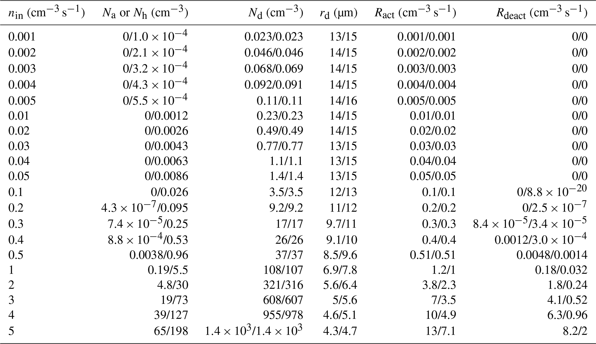
Table 2 summarizes the spatially and temporally averaged cloud microphysical properties for n_in≤5.0 cm⁻³ s⁻¹ when the scaling laws work reasonably well. Those variables include aerosol (when using the CL_CCN scheme)/haze (when using the CL_Haze scheme) number concentration (N_a/N_h), cloud droplet number concentration (N_d), mean cloud droplet radius (r_d), droplet activation rate (R_act), and deactivation rate (R_deact). The droplet activation rate represents the number of newly formed cloud droplets per cubic centimeter per second, while the deactivation rate represents the reverse process. Note that the net activation rate (R_act−R_deact, the last two columns in Table 2) is close to n_in (the first column in Table 2) for each case suggesting that the cloud reaches a quasi-steady state. It is worth mentioning that although the simulated cloud properties using the two schemes are similar, unactivated particle concentration (N_a or N_h), R_act, and R_deact are quite different for n_in≥1.0 cm⁻³ s⁻¹. Our results suggest that haze–cloud interactions are important in the fast microphysics regime. The transition from the slow to the fast microphysics regime occurs when haze particles become important: $N_{\mathrm{h}}/N_{\mathrm{d}}>\mathrm{5}$ % and $R_{\mathrm{deact}}/R_{\mathrm{act}}>\mathrm{3}$ % for n_in≥1.0 cm⁻³ s⁻¹ (Fig. 4).

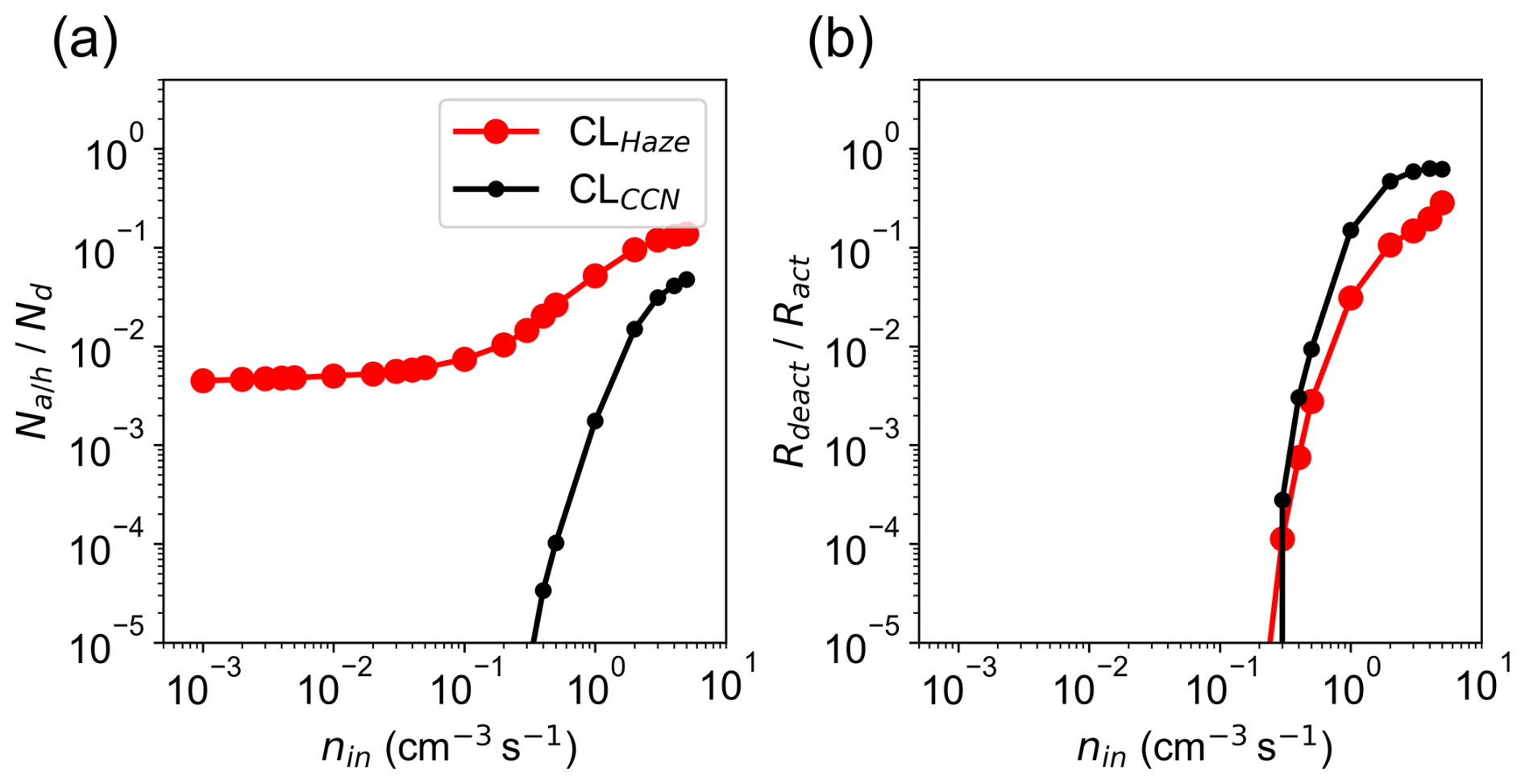
Figure 4 (a) The ratio of the unactivated particle number concentration to the cloud droplet number concentration for different aerosol injection rates (n_in). Unactivated particles are aerosol particles when using the CL_CCN scheme or haze particles when using the CL_Haze scheme. (b) The ratio of deactivation to activation rate for different n_in.

Shaw et al. (2023) predicted that the transition from slow to fast microphysics regimes occurs at Da ≈1. Here Da is the Damköhler number, defined as the ratio of turbulent mixing time (τ_m) to phase relaxation time (τ_p) (see Eq. 1 in Lehmann et al., 2009). τ_p is inversely proportional to the product of N_d and r_d, which can be determined from our simulation results. Take n_in=0.1 cm⁻³ s⁻¹ as an example, τ_p≈70 s, calculated from N_d=3.5 cm⁻³ and r_d=12 µm based on Table 2 (using Eq. 18 in Korolev and Mazin, 2003). The apparent transition between slow and fast regimes as shown in Fig. 1 provides an opportunity to estimate τ_m, which is about 70 s for our boundary conditions (e.g., 20 K difference in top and bottom temperature), if we assume the transition occurs at Da ≈1. However, this value is larger than another estimate of τ_m via ${\mathit{\tau }}_{\mathrm{m}}=H/v_{\mathrm{air}}$. Here, H=1 m is the chamber height, and v_air≈0.1 m s⁻¹ is the characteristic air speed in the chamber based on LESs, leading to τ_m on the order of 10 s. It is also larger than another estimate of ${\mathit{\tau }}_{\mathrm{m}}=H^{\mathrm{2}/\mathrm{3}}/{\mathit{ϵ}}^{\mathrm{1}/\mathrm{3}}\approx \mathrm{6}$ s, where ϵ is the energy dissipation rate (about 0.005 m² s⁻³ from the simulation).

3.2 Haze–cloud interactions in the polluted conditions

Figure 1c and d show that N_d and q_l do not follow the aforementioned scaling laws for n_in≥10 cm⁻³ s⁻¹. In this section, we explore the reason for this departure and show that haze–cloud interaction in these extremely polluted conditions can lead to some new microphysics regimes, including cloud oscillation, cloud collapse, and haze only.

3.2.1 Cloud oscillation

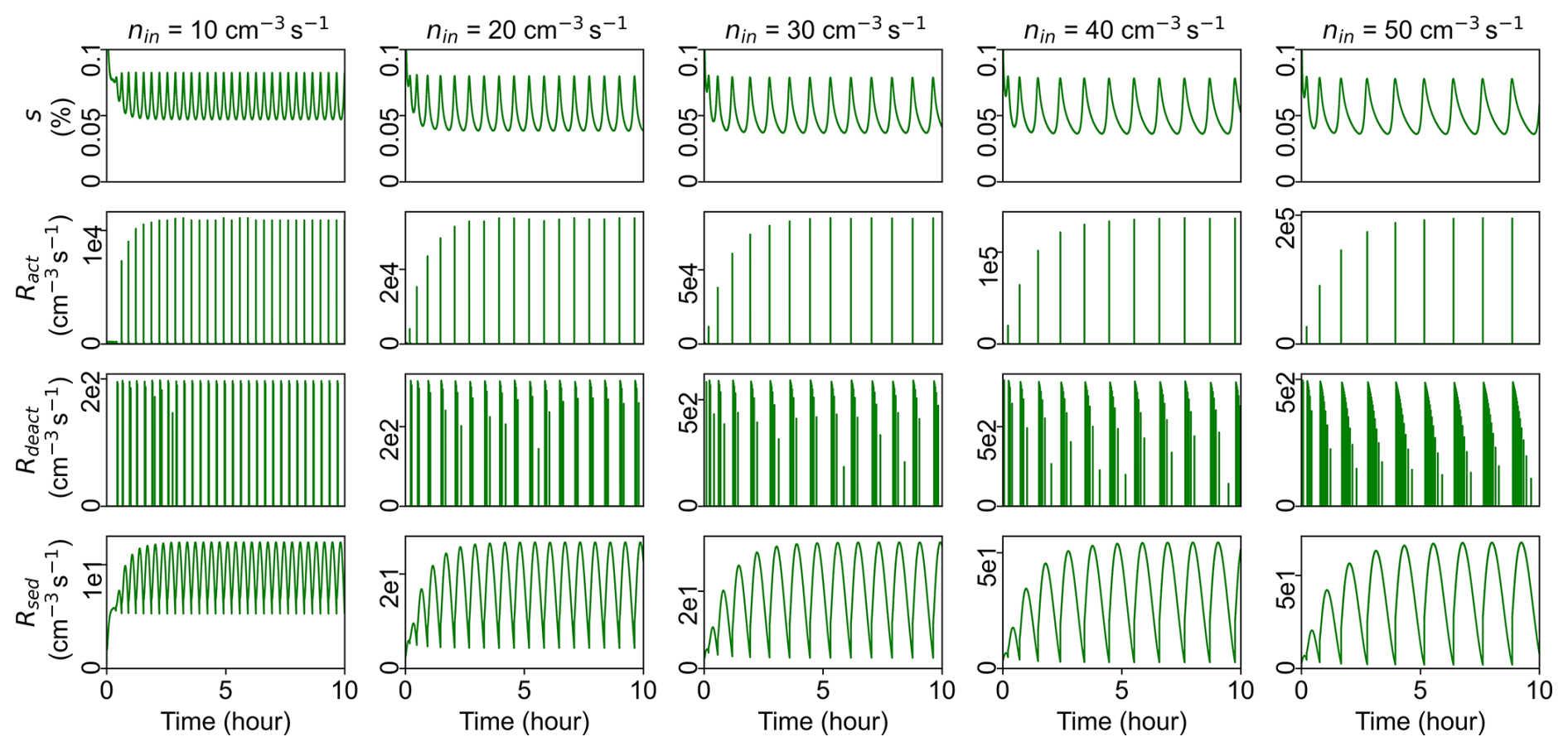
One possible reason for the observed departure for N_d and q_l in the polluted conditions (n_in≥10 cm⁻³ s⁻¹) is that the cloud does not reach a steady state after 1 h. To rule out this possibility, we extend the simulations of the largest five n_in (10, 20, 30, 40, 50 cm⁻³ s⁻¹) to a total simulation time of 10 h. Figure 5 shows the time series of domain-averaged q_l, q_c, N_d, N_a (for the CL_CCN scheme), N_h (for the CL_Haze scheme), total particle concentration (N_T), and r_d. Note that q_l≥q_c and $N_{\mathrm{T}}=N_{\mathrm{d}}+N_{\mathrm{h}}$ when using the CL_Haze scheme, and the difference (q_l−q_c) is haze water mixing ratio (q_h), while q_l=q_c and $N_{\mathrm{T}}=N_{\mathrm{d}}+N_{\mathrm{a}}$ when using the CL_CCN scheme. Results show that q_l, N_d, and r_d always reach a steady state when using the CL_CCN scheme. Note that N_a and N_T increase with time for n_in≥ 40 cm⁻³ s⁻¹. This is because the sink of aerosol due to droplet activation is smaller than the source of aerosol due to aerosol injection, and thus aerosol particles accumulate. When using the CL_Haze scheme, the cloud reaches a steady state for an aerosol injection rate of 10 cm⁻³ s⁻¹, where q_l is dominated by q_c. In contrast, for n_in≥20 cm⁻³ s⁻¹, cloud microphysical properties (such as q_l, q_c, N_d, r_d) oscillate. The oscillation period increases as n_in increases, and the periods are 15, 20, 25, and 30 min for n_in=20, 30, 40, and 50 cm⁻³ s⁻¹. Meanwhile, the oscillation amplitude increases with n_in. N_T has a much smaller oscillation magnitude compared with N_d and N_h, suggesting that oscillations of N_h and N_c are out of phase. The local maximum of N_d corresponds to the local minimum of N_h, indicating the burst of droplet formation is due to the activation of a large number of haze particles. The ratio of q_h (i.e., q_l–q_c) to q_l increases with n_in, and it can be up to 30 % for n_in=50 cm⁻³ s⁻¹. Note that the oscillation of the mean r_d is mainly due to droplet activation/deactivation, not due to the physical growth/evaporation of cloud droplets. For example, the rapid formation of numerous small cloud droplets decreases the mean r_d accordingly.

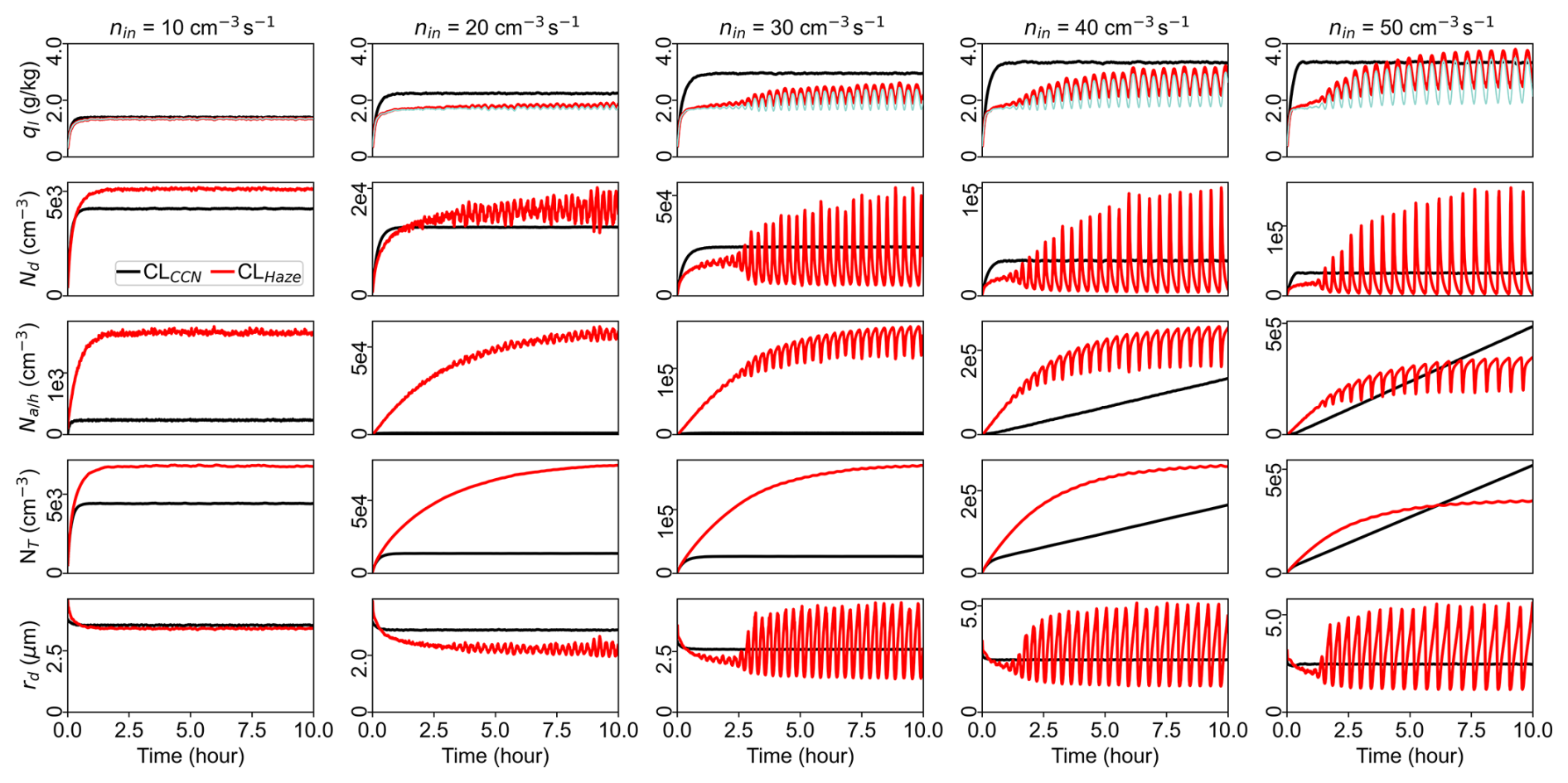
Figure 5 Time series of domain-averaged q_l (first row), N_d (second row), N_a or N_h (third row), N_T (fourth row), and r_d (fifth row) for five different n_in: 10, 20, 30, 40, and 50 cm⁻³ s⁻¹. The light-blue line in the first row represents the cloud water mixing ratio (q_c) when using the CL_Haze scheme.

Figure 6 shows time series of domain-averaged activation rate (R_act), deactivation rate (R_deact), supersaturation (s), standard deviation of supersaturation (σ_s), and surface precipitation rate (P). Here surface precipitation refers to the sedimentation of cloud droplets at the bottom surface. Results show that oscillations of bulk cloud properties when using the CL_Haze scheme, as shown in Fig. 5, are associated with oscillations of process rates, like R_act, R_deact, and P. It is interesting to see that s is close to s_crit (about 0.08 %) when using the CL_Haze scheme, while s decreases with n_in and approaches 0 when using the CL_CCN scheme. This is because the cloud system is buffered by a huge number of cloud droplets in the polluted condition and s should be close to the equilibrium supersaturation over droplets. This equilibrium supersaturation is s_crit when using the CL_Haze scheme where solute and curvature effects are considered, but it is 0 when using the CL_CCN scheme. Because σ_s is much smaller than s_crit at high injection rates, droplet activation is mainly controlled by the mean s. The oscillation of s around the s_crit leads to the oscillation of droplet activation and further causes the oscillation of cloud properties.

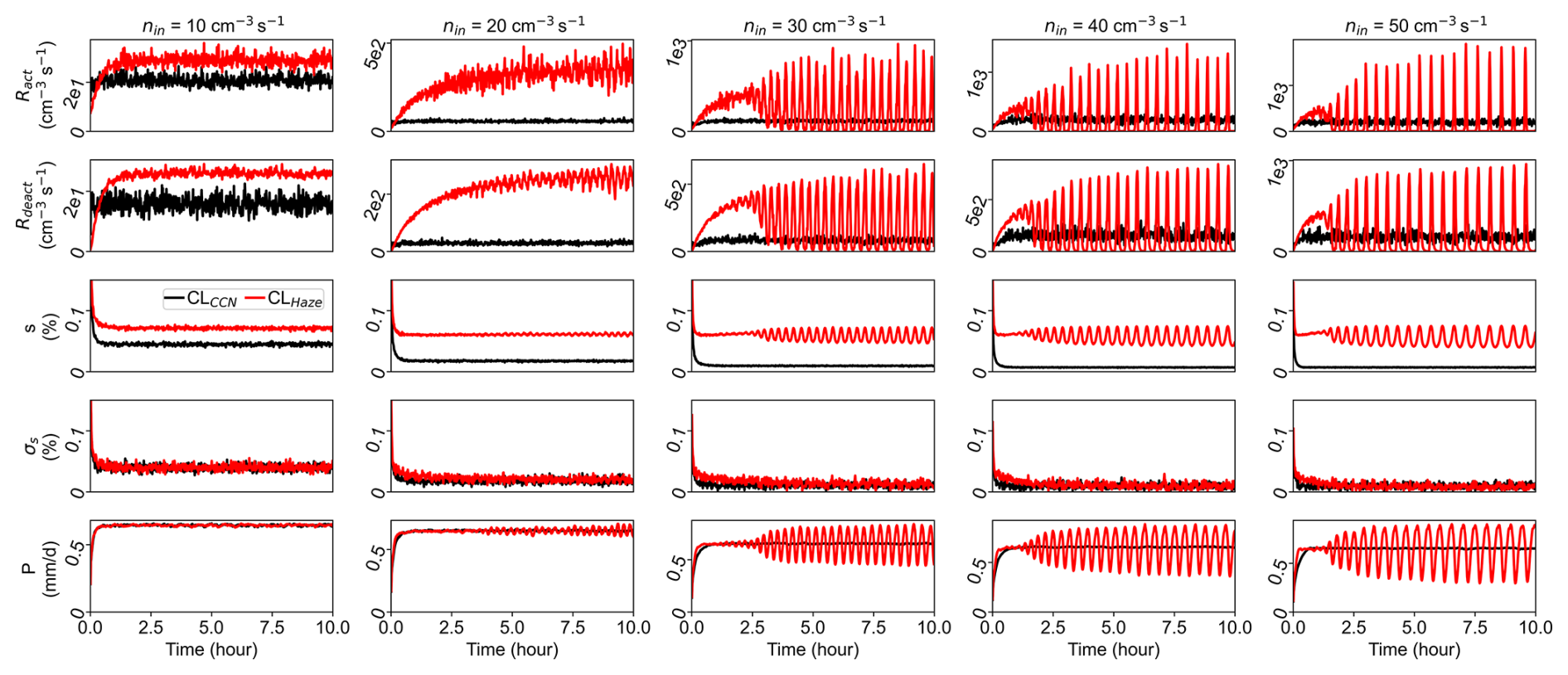
Figure 6 Same cases in Fig. 5, time series of domain-averaged R_act (first row), R_deact (second row), s (third row), σ_s (fourth row), and surface precipitation rate P (fifth row) for five different n_in: 10, 20, 30, 40, and 50 cm⁻³ s⁻¹.

Figure 7 shows the time evolution of mean profiles of cloud properties in the last hour of the simulation for n_in=40 cm⁻³ s⁻¹. We note that q_c and q_h oscillate out of phase (Fig. 7a vs. d), while q_l is mainly influenced by q_c (Fig. 7g). Larger q_c (q_h) corresponds to smaller N_d (N_h) and vice versa (Fig. 7a vs. b and d vs. e). The anti-correlation between q_c and N_d is opposite to their scaling relationships in the slow and fast microphysics, which are q_c∼N_d and $q_{\mathrm{c}}\sim N_{\mathrm{d}}^{\mathrm{2}/\mathrm{5}}$, respectively (Shaw et al., 2023). The sharp increase in N_d (Fig. 7b) corresponds to a larger activation rate (Fig. 7c) due to the enhanced supersaturation (Fig. 7i), while the decrease in N_d corresponds to a larger deactivation rate and a smaller supersaturation. To better show the low value of R_act and R_deact, we constrain the range of R_act and R_deact to values below 240 cm⁻³ s⁻¹ if their values are larger than it when plotting Fig. 7c and f. It can be seen that deactivation occurs in a much larger region (i.e., outside the top and bottom surfaces) and over a longer period within one cycle. However, the peak of R_act is larger than the peak of R_deact (see Fig. 6 first and second rows). The net activation rate (R_act−R_deact) averaged over one cycle should still be positive so that sedimentation is balanced by the net activation.

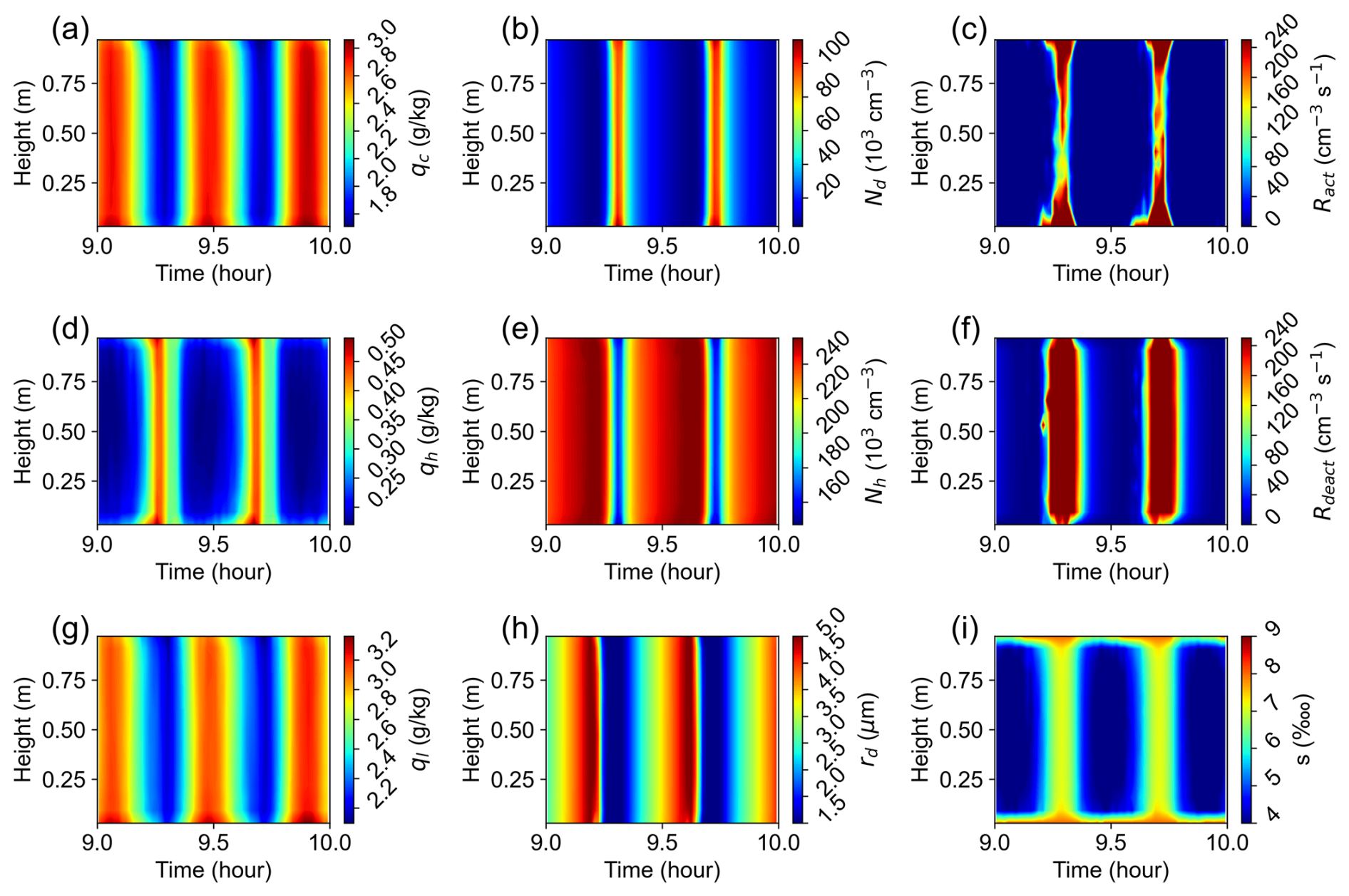
Figure 7 Time evolution of mean profiles of (a) cloud water mixing ratio, q_c; (b) cloud droplet number concentration, N_d; (c) activation rate, R_act; (d) haze water mixing ratio, q_h; (e) haze number concentration, N_h; (f) deactivation rate, R_deact; (g) total water mixing ratio, q_l; (h) droplet radius, r_d; and (i) supersaturation, s, for n_in=40 cm⁻³ s⁻¹ between 9 and 10 h when using the CL_Haze scheme. It is the last simulation hour of Fig. 5, second column.

To further explore the mechanism of the oscillation, we pick one oscillation cycle for n_in=40 cm⁻³ s⁻¹. Figure 8 shows the phase diagram of four pairs of variables: N_h vs. N_d, q_h vs. q_c, q_h vs. N_h, and q_c vs. N_d. Each circle in the figure represents the domain-averaged value at one time and its color represents the domain-averaged supersaturation with the unit of , 1 per 10 000. The size of the circle represents the mean droplet radius in a relative way: a larger circle means a larger r_d. The oscillation behavior can be explained by the circulation in the phase diagram. Taking Fig. 8d as an example: start from the lower left corner where q_c and N_d are low, s is high, and r_d is large. When s>s_crit (s_crit≈8  in this study), a huge number of droplets are activated leading to a sharp increase in N_d. Newly formed cloud droplets significantly decrease the mean r_d, and they grow in slightly supersaturated conditions, leading to an increase in q_l and a decrease in s. Shortly thereafter, N_d decreases because droplet activation is suppressed when s<s_crit, and meanwhile, droplets are lost due to sedimentation and deactivation. Note that droplet loss is dominated by deactivation, and deactivation is driven by the mean supersaturation rather than supersaturation fluctuation because s oscillates around s_crit while σ_s is much smaller than s_crit as shown in Fig. 6. Droplet deactivation causes a recovery of N_h and an increase in q_h (Fig. 8a, b). The decrease in N_d finally results in a decrease in q_l and an increase in s. When s>s_crit, another period starts. Note that droplet activation leads to an increase in N_d and a decrease in N_h simultaneously, thus causing the perfect anticorrelation between N_h and N_d (Fig. 8a). In contrast, mass and number concentrations (either q_h vs. N_h or q_c vs. N_d) peak at different times because it takes time for droplets/haze to grow. It is interesting to see that the oscillation evolves with time counterclockwise in the $q_{\mathrm{h}}--N_{\mathrm{h}}$ diagram (Fig. 8c) and the $q_{\mathrm{c}}--N_{\mathrm{d}}$ diagram (Fig. 8d), suggesting that the change in number concentration is ahead of the change in mass mixing ratio in their phases, analogous to a predator–prey dynamical system.

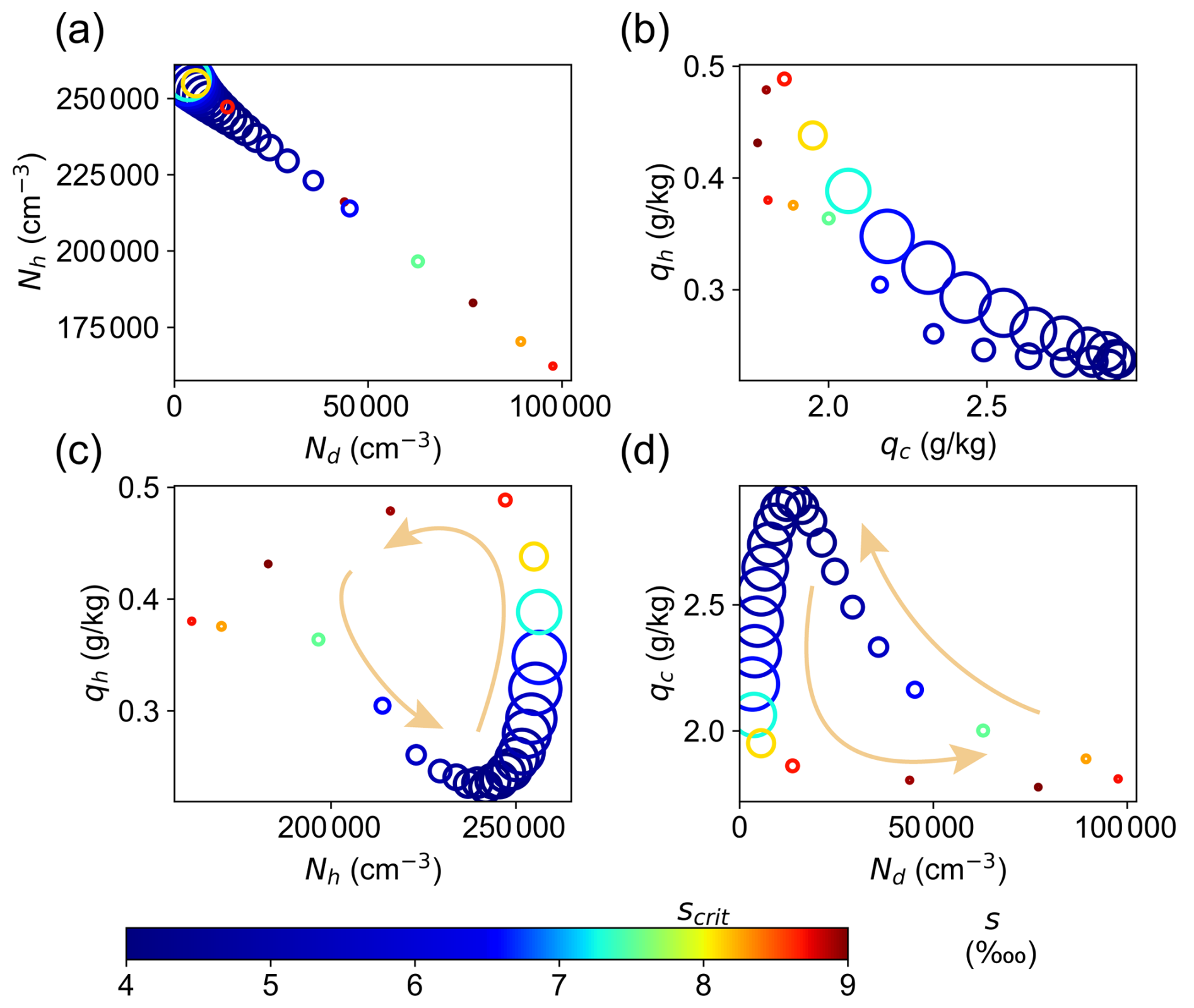
Figure 8 The relationship between domain-averaged (a) N_h vs. N_d, (b) q_h vs. q_c, (c) q_h vs. N_h, and (d) q_c vs. N_d over one cycle of cloud oscillation at n_in=40 cm⁻³ s⁻¹. The size of the circle represents the mean droplet radius in a relative way; e.g., a larger circle means a larger r_d. Its color stands for the domain-averaged supersaturation with a unit of , 1 per 10 000. The arrows in (c) and (d) represent its time evolution in one cycle.

3.2.2 Cloud oscillation in a box model

To make sure the oscillation is physical and not due to numerical artifacts from using an Eulerian-based bin microphysics scheme, we develop a box model using a particle-based microphysics approach to simulate a cloud in a convection chamber. The particle-based treatment, analogous to the Lagrangian droplet method, directly calculates and tracks the time evolution of droplet size. The well-mixed cloud system can be described by a set of differential equations detailed below.

Following Shaw et al. (2023), the time derivative of mean air temperature can be expressed as

$$\begin{array}{}\text{(1)}& {\displaystyle \frac{\mathrm{d}T}{\mathrm{d}t}}={\displaystyle \frac{T_{\mathrm{0}}-T}{{\mathit{\tau }}_{\mathrm{m}}}}+{\displaystyle \frac{L}{c_p}}{\displaystyle \frac{\mathrm{d}{q}_{\mathrm{l}}}{\mathrm{d}t}}{|}_{\mathrm{diff}},\end{array}$$

where T₀ is the reference temperature, which equals the mean temperature in the chamber without cloud droplets. L is the latent heat of vaporization of water, and c_p is the specific heat of air. τ_m is the mixing timescale, which quantifies how efficient T can be restored to T₀. Similarly, the time derivative of the water vapor mixing ratio is expressed as

$$\begin{array}{}\text{(2)}& {\displaystyle \frac{\mathrm{d}{q}_{\mathrm{v}}}{\mathrm{d}t}}={\displaystyle \frac{q_{\mathrm{v}\mathrm{0}}-q_{\mathrm{v}}}{{\mathit{\tau }}_{\mathrm{m}}}}-{\displaystyle \frac{\mathrm{d}{q}_{\mathrm{l}}}{\mathrm{d}t}}{|}_{\mathrm{diff}},\end{array}$$

where q_v0 is the reference water vapor mixing ratio, which equals the mean water vapor mixing ratio in a cloud-free condition assuming both top and bottom surfaces are saturated with respect to water. The last terms in Eqs. (1) and (2) represent the impact of vapor diffusional growth ($\mathrm{d}{q}_{\mathrm{l}}/\mathrm{d}t{|}_{\mathrm{diff}}$) of droplets on T and q_v, respectively.

To be consistent with the model setup of large-eddy simulations, monodisperse dry aerosol particles with radii of 62.5 nm are added at a constant rate using a particle-based super droplet method. Specifically, one new super particle (hereafter referred to as particle) is added at a constant rate: every second for n_in≤5 cm⁻³ s⁻¹ or every 20 s for the largest five n_in to save computational time. Each particle represents numerous real particles per unit volume. We refer to this as multiplicity, denoted hereafter as n_i, which represents the concentration of a particle with an index of i. Note that the multiplicity in this study is different from that in Lagrangian microphysics schemes (e.g., Shima et al., 2009; Hoffmann et al., 2015) in which it represents multiple number (instead of concentration) of identical droplets represented by the Lagrangian particle/superdroplet. The growth rate of droplet radius with an index of i is given by

$$\begin{array}{}\text{(3)}& {\displaystyle \frac{\mathrm{d}{r}_i}{\mathrm{d}t}}={\displaystyle \frac{G}{r_i}}\left(s-{\displaystyle \frac{A}{r_i}}+{\displaystyle \frac{B}{r_i^{\mathrm{3}}}}\right),\end{array}$$

where G is the growth factor, and s is the supersaturation depending on both T and q_v. $A/r_i$ and $B/r_i^{\mathrm{3}}$ are curvature and solute effects, respectively, in which A and B are constant for given thermodynamic and aerosol conditions (Eq. 6.6 in Rogers and Yau, 1996). The change in liquid water mixing ratio, which is linked to the last terms in Eqs. (1) and (2), can be calculated as the sum of mass change of all droplets,

$$\begin{array}{}\text{(4)}& {\displaystyle \frac{\mathrm{d}{q}_{\mathrm{l}}}{\mathrm{d}t}}{|}_{\mathrm{diff}}={\displaystyle \frac{\mathrm{4}\mathit{\pi }{\mathit{\rho }}_{\mathrm{l}}}{{\mathit{\rho }}_{\mathrm{a}}}}\sum _i{n}_i{r}_i^{\mathrm{2}}{\displaystyle \frac{\mathrm{d}{r}_i}{\mathrm{d}t}}.\end{array}$$

Here ρ_a and ρ_l are air and liquid water densities, respectively.

Equations (1)–(4) are the governing equations to describe the bulk properties of a well-mixed cloud in a convection chamber. We use an ordinary differential equation solver to solve the above set of nonlinear and stiff equations (Brown et al., 1989). The total number of equations in the system depends on the number of particles. For example, if we have 100 particles at a given moment, the total number of equations to be solved is 102 (100 for r_i, 1 for T, and 1 for q_v). The same solver has been used in adiabatic cloud parcel models to properly calculate the growth of haze particles and the droplet activation process in the real atmosphere (Xue and Feingold, 2004; Chen et al., 2016; Yang et al., 2016).

Without sedimentation, the number of particles in the system would increase with time due to continuous injection, which eventually makes the system numerically unsolvable. In reality, the number of particles increases with time at the beginning, but it could reach a steady state if the rate of increase in particles due to injection is balanced by its loss rate due to sedimentation. To represent the impact of gravitational sedimentation, n_i decreases with time as

$$\begin{array}{}\text{(5)}& \mathit{\delta }{n}_i=n_i\left(\mathrm{1}-\exp \left[-{\displaystyle \frac{\mathit{\delta }t}{{\mathit{\tau }}_{\mathrm{sed}}\left(r_i\right)}}\right]\right)\approx n_i{\displaystyle \frac{\mathit{\delta }t}{{\mathit{\tau }}_{\mathrm{sed}}\left(r_i\right)}},\end{array}$$

where δt is set to be 1 s, and δn_i is the decreased amount of multiplicity of a particle with the index of i. τ_sed is the characteristic sedimentation time of a droplet with a radius of r_i in a convection cloud chamber,

$$\begin{array}{}\text{(6)}& {\mathit{\tau }}_{\mathrm{sed}}\left(r_i\right)={\displaystyle \frac{H}{v_{\mathrm{t}}\left(r_i\right)}}.\end{array}$$

Here H is the chamber height of 1 m, and v_t is the terminal velocity of a droplet with a radius of r_i. If n_i is smaller than a threshold of 10⁻¹⁰ cm⁻³, we remove that particle.

We conduct a total of 25 cases with the same forcing (i.e., T₀, q_v0, and τ_m) but different n_in, which are the same as those used in previous large-eddy simulations. For a given n_in, the multiplicity of a newly added particle (n_i0) and the injection frequency are determined such that their product equals n_in. For example, injection of a particle with n_i0=0.5 cm⁻³ every second corresponds to n_in=0.5 cm⁻³ s⁻¹, while injection of a particle with n_i0=200 cm⁻³ every 20 s corresponds to n_in=10 cm⁻³ s⁻¹. T₀ and q_v0 are set to be 290 K and 13.9 g kg⁻¹, corresponding to a supersaturation of 15 % in the absence of all hydrometeors. This setup is consistent with the cloud-free humid condition in a convection chamber with a top temperature of 280 K and a bottom temperature of 300 K, with both surfaces saturated with respect to water. τ_m is set to be 165 s, such that the steady-state s from the box model (Fig. 9a) agrees with that from the LES (Fig. 1a). Note that the value of τ_m used here is not the same as the estimated τ_m (∼70 s) for Da=1 based on LES results above, but they are the same order of magnitude.

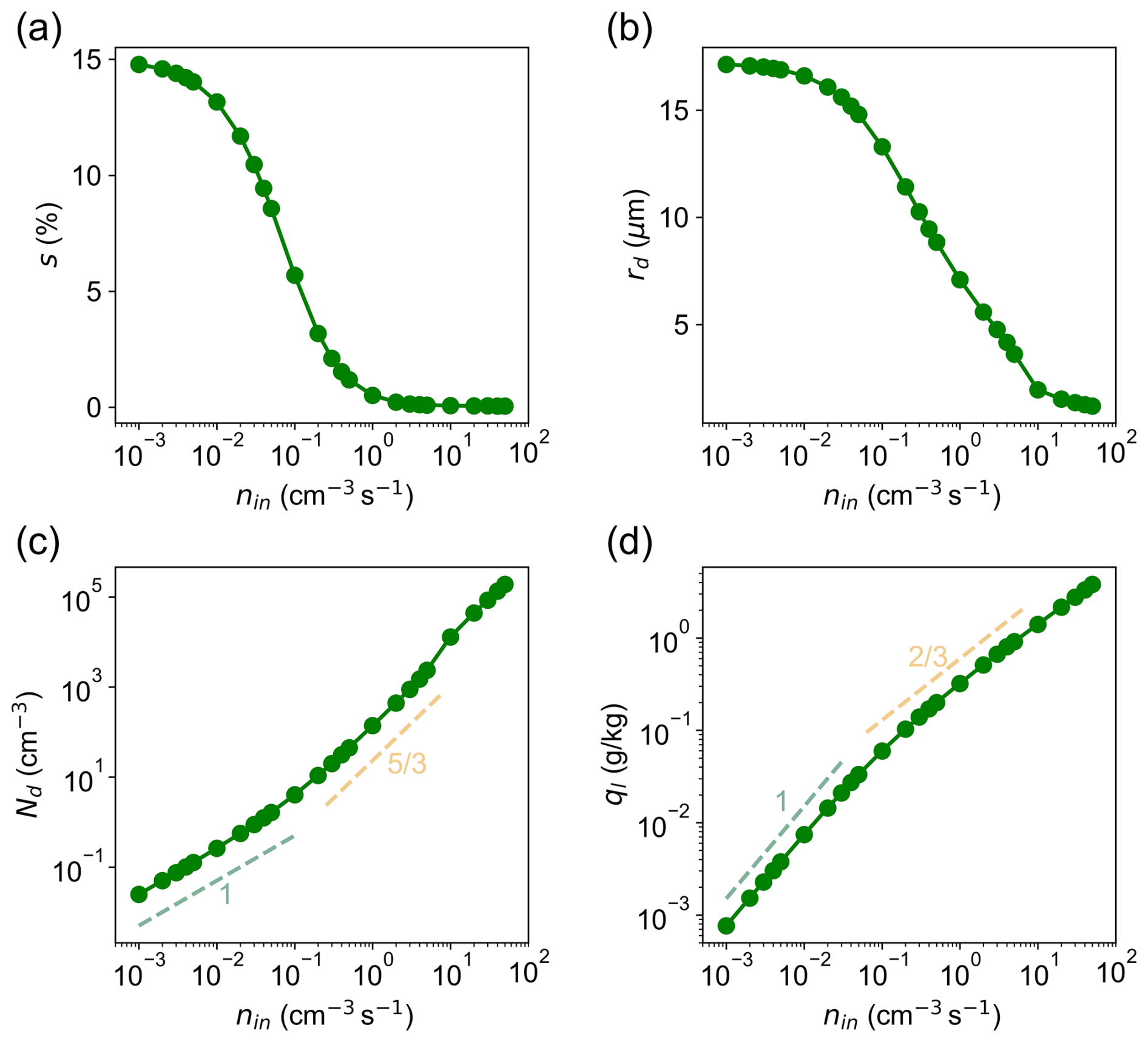
Figure 9 Impact of n_in on (a) supersaturation s, (b) mean droplet radius r_d, (c) droplet number concentration N_d, and (d) liquid water mixing ratio q_l based on a box model using a particle-based microphysics approach. Cloud oscillation occurs for the five largest n_in values (10, 20, 30, 40, 50 cm⁻³ s⁻¹), as shown in Fig. 10. For those cases, s, r_d, N_d, and q_l are averaged over one cycle. The light-green and yellow-colored dashed lines in (c) and (d) are scaling relationships based on Shaw et al. (2023) for slow and fast regimes, respectively.

Results show that the impact of n_in on cloud properties based on the box model is consistent with those from LESs (compare Fig. 9 vs. Fig. 1). Slow and fast microphysics regimes are also captured by the box model (Fig. 9c, d). It is encouraging to see that the transition between slow and fast microphysics regimes occurs at around n_in of 0.1 cm⁻³ s⁻¹, which agrees well with LESs. The box model also captures cloud oscillation for the largest five n_in (10, 20, 30, 40, 50 cm⁻³ s⁻¹), as shown in Figs. 10 and 11. The oscillation frequency decreases with the increase in n_in, which is consistent with LES results (Fig. 5). Note that, for cloud oscillation cases, s, r_d, N_d, and q_l in Fig. 9 are averaged over one cycle. It is interesting to see that N_d vs. n_in and q_l vs. n_in agree better with the aforementioned scaling laws in the fast microphysics regime, compared with LESs (compare Fig. 9c, d vs. Fig. 1c, d). This might be due to the bias in representing droplet distribution when using a limited number of discretized bins in polluted conditions or the systematic difference between a 3-D LES and a box model.

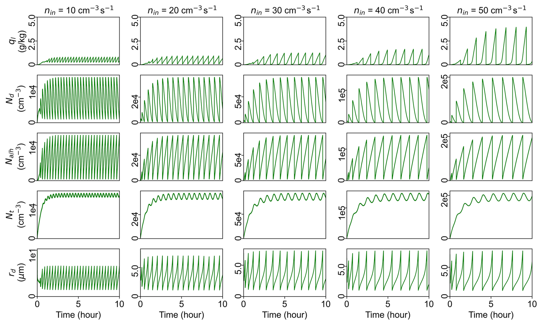
Figure 10 Time series of q_l (first row), N_d (second row), N_h (third row), N_t (fourth row), and r_d (fifth row) from a box model using a Lagrangian microphysics approach for the five largest n_in: 10, 20, 30, 40, 50 cm⁻³ s⁻¹.

Figure 11 Similar to Fig. 10, time series of s (first row), R_act (second row), R_deact (third row), and R_sed (fourth row) from a box model using a Lagrangian microphysics approach for the five largest n_in: 10, 20, 30, 40, 50 cm⁻³ s⁻¹.

3.2.3 Origin of cloud oscillation

Results from LES and box models show the existence of cloud oscillation at high n_in, indicating that cloud oscillation is physically plausible, not due to numerical artifact. In this subsection, we discuss the physical origin of cloud oscillation and explain why the CL_Haze scheme can simulate cloud oscillation, while the CL_CCN scheme fails.

Time series of s shown in Figs. 6 and 11 provide more physical insights of cloud oscillation. The direct reason for cloud oscillation is that s oscillates around s_crit when using the CL_Haze scheme. To be clear, cloud oscillation mentioned in this study represents the oscillation of cloud bulk statistical properties. It is the oscillation of the whole well-mixed cloud system, not an individual droplet. The physical origin of cloud oscillation is due to the nonlinear interactions between haze and cloud droplets in a dynamic system:

1. First, the supersaturation s in the system is very close to s_crit, and most of the time s<s_crit. This can happen in a heavily polluted condition where there are many haze particles.

2. There is a forcing in the system to maintain the supersaturation. In the Pi chamber, the forcing is due to the temperature difference between the top and bottom surfaces. In the real atmosphere, the forcing can be due to adiabatic cooling (e.g., in a rising cloud parcel) or radiative cooling (e.g., radiation fog).

3. When s>s_crit, a huge number of haze particles activate to cloud droplets and the consumption of water vapor due to droplet condensational growth leads to s<s_crit.

4. Under s<s_crit conditions, droplet activation is suppressed and droplet concentration decreases due to droplet deactivation and sedimentation.

5. Meanwhile, haze number concentration increases due to continuously aerosol injection and droplet deactivation.

6. s increases with the decrease in the sink of water vapor due to fewer cloud droplets and more haze particles, and when s>s_crit, another cycle starts. In contrast, s approaches 0 when using the CL_CCN scheme (black line in the third row of Fig. 6), suggesting that droplet activation is strongly suppressed in the bulk region.

Additionally, σ_s decreases with n_in and approaches 0 due to the buffering effect of cloud droplets under polluted conditions (Fig. 6, fourth row). This suggests that droplet activation is controlled by the mean supersaturation instead of supersaturation fluctuation. This is why even though turbulence is not considered, the box model (Fig. 9) and the theoretical model (developed in Shaw et al., 2023) can still predict the scaling relationships in fast and slow microphysics regimes that are consistent with large-eddy simulations (Fig. 1) and Pi chamber experiments (Fig. 7 in Shaw et al., 2023). The nice performance of the theoretical model and the box model suggests that turbulence is not the direct factor in generating various microphysics regimes, including provoking cloud oscillation. As long as the cloud is well mixed (due to turbulence), various microphysics regimes (e.g., slow, fast, oscillation) can occur under different aerosol injection rates (for monodisperse aerosols like in this study).

It is interesting to see that droplet deactivation can still occur even though s is always positive in the box model (Fig. 11). This is also likely to be true in LESs when using the CL_Haze scheme, in which s oscillates around s_crit and σ_s≪s_crit. One question is what drives droplet deactivation in a supersaturated environment. Here, droplet deactivation occurs due to the curvature effect: although haze particles can be activated to droplets when s>s_crit, the subsequent decrease in s (like s oscillation in our case) can lead to droplet deactivation when s is smaller than the saturated saturation ratio over small cloud droplets (see green line in Fig. 1 of Nenes et al., 2001). Droplet deactivation in supersaturated conditions occurs when the phase relaxation time is much shorter than the droplet activation time. This phenomenon is closely relevant to the onset of the catastrophe discussed in Arabas and Shima (2017). In addition, there is one difference in handling droplet deactivation between the CL_CCN and the CL_Haze schemes. If droplets are deactivated, they go back to the dry aerosol category when using the CL_CCN scheme. When using the CL_Haze scheme, droplets stay as haze particles which can still consume water vapor and contribute to liquid water content. The latter has feedback in s which is critical to trigger cloud oscillation that we will discuss next.

When s<s_crit, droplet activation is suppressed in the bulk region. This is true for both CL_Haze and CL_CCN schemes. However, when using the CL_Haze scheme, the contribution of haze water content to the total liquid water content increases under this condition (s<s_crit) due to continuous aerosol injection and droplet deactivation (as discussed above). The sink of water vapor via condensational growth decreases due to the decrease in cloud droplet concentration, which can lead to an increase in s, considering that the source of water vapor from chamber surfaces is constant. When s>s_crit, droplet activation is active again. In contrast, when using the CL_CCN scheme, haze water content is not considered, and cloud droplet content is equivalent to liquid water content. In addition, both s and σ_s are buffered to approach 0 under polluted conditions, and there is no restoring force to increase s.

3.2.4 Cloud collapse

For the simulations above, the side walls are set to be saturated with respect to water. In reality, the side walls in the Pi chamber could be subsaturated, which could enhance droplet deactivation. To investigate the impact of side wall humidity (RH_wall) on cloud oscillation, we set RH_wall to be 90 %, 70 %, 50 %, and 30 % for n_in=20 cm⁻³ s⁻¹. This is similar to the entrainment of subsaturated air into a natural cloud. Figure 12 shows the time series of domain-averaged q_l, N_d, N_a or N_h, N_T, and r_d, while Fig. 13 shows the corresponding R_act, R_deact, s, σ_s, and P (as Figs. 5 and 6). Results indicate that q_l decreases with RH_wall (Fig. 12 first row). This is because subsaturated side walls serve as a water sink to evaporate droplets and thus enhance haze–cloud interactions. Note that q_h can be as large as q_c (e.g., for RH_wall of 30 % at the end of the simulation), which cannot be captured when using the CL_CCN scheme. The cloud always reaches a steady state when using the CL_CCN scheme. In contrast, when using the CL_Haze scheme, the cloud oscillates for RH_wall of 90 and 70 %, but it can reach a steady state for RH_wall of 50 %, and more interestingly, it tends to collapse for RH_wall of 30 % (Fig. 12 second row). Here we define “cloud collapse” as the significant decrease in N_d at low RH_wall conditions. It is also clear to see that the bulk s is negative in the cloud collapse regime (fourth row in Fig. 13). Note that the cloud does not dissipate completely because q_c still reaches a steady state, probably due to droplet activation near the top and bottom surfaces where the local s can be still larger than s_crit (similar to the high s observed near the surface in Wang et al. (2024a).

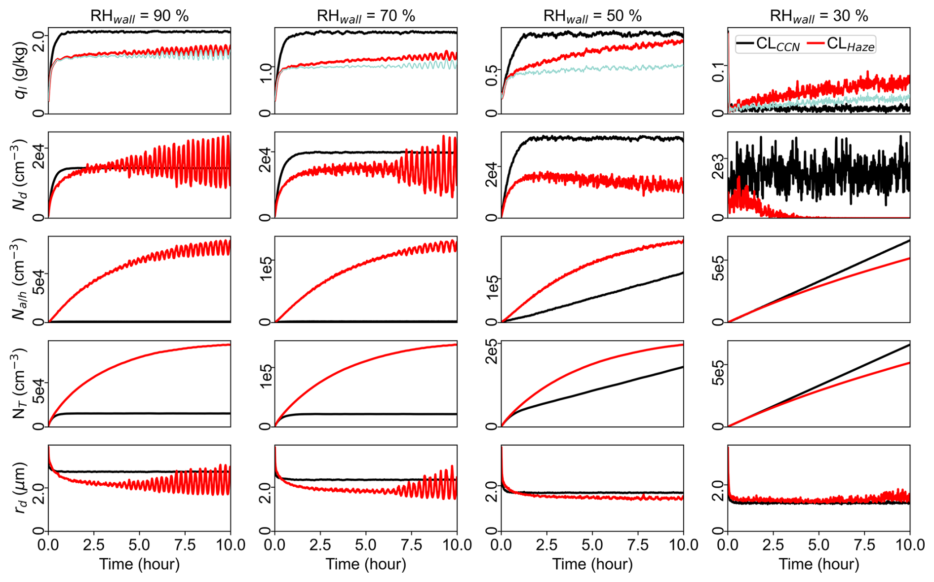
Figure 12 Time series of domain-averaged q_l (first row), N_d (second row), N_a or N_h (third row), N_T (fourth row), and r_d (fifth row) at a n_in of 20 cm⁻³ s⁻¹ with four different size wall relative humidity levels, RH_wall = 90 %, 70 %, 50 %, and 30 %. The light-blue line in the first row represents the cloud water mixing ratio (q_c) when using the CL_Haze scheme.

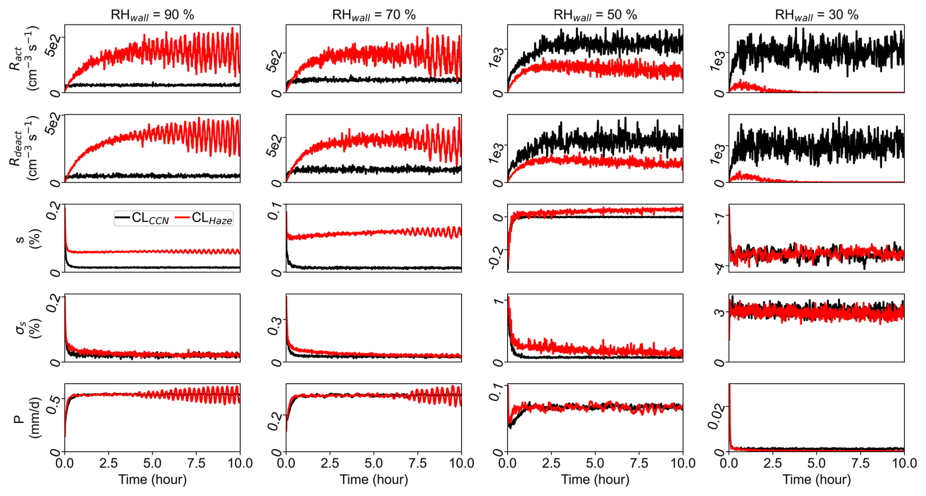
Figure 13 Same cases in Fig. 12 but showing time series of domain-averaged R_act (first row), R_deact (second row), s (third row), σ_s (fourth row), and P (fifth row) at a n_in of 20 cm⁻³ s⁻¹ with four different size wall relative humidity levels, RH_wall = 90 %, 70 %, 50 %, and 30 %.

Our results suggest that cloud oscillation and cloud collapse result from haze–cloud interactions in a homogeneous and inhomogeneous supersaturation field, respectively. When the side walls are close to be saturated, the supersaturation field is almost homogeneous everywhere in the chamber except very close to the top and bottom surfaces. Such a homogeneous supersaturation field allows synchronized droplet activation or deactivation to occur throughout the entire chamber and thus leads to cloud oscillation as explained above and Fig. 8. However, when the side walls are considerably drier, the supersaturation field in the chamber is not homogeneous: air close to the side wall is subsaturated while air close to the center, top, and bottom surfaces is supersaturated. Such an inhomogeneous field causes droplet activation in one region and deactivation in another region. For a moderate dry side wall (i.e., RH_wall of 50 %), a steady state might be reached if the net activation rate is balanced by the droplet sedimentation rate. For an extremely dry side wall (i.e., RH_wall of 30 %), the chamber can be considered a machine to efficiently transfer cloud droplets to haze particles over time, leading to the cloud collapse.

3.2.5 Haze-only regime

So far, our results show that besides slow and fast microphysics regimes, there exists a cloud oscillation regime at a high aerosol injection rate due to haze–cloud interactions. In the oscillation regime, the oscillation frequency decreases and the haze number concentration increases as n_in increases. It raises a question of what would happen if n_in is extremely large. Would there be another regime in which there are only haze particles and no cloud droplets? Here, we develop a simple model to investigate the properties of a postulated haze-only regime.

Let us assume only haze particles exist in the chamber at an extremely high aerosol injection rate. Following the approach of Shaw et al. (2023) (Eqs. 56 and 57 therein), in the steady state, the mean air temperature would be higher than the reference temperature (i.e., T₀, same as in our Eq. 1) due to latent heat release from the formation of haze particles,

$$\begin{array}{}\text{(7)}& T=T_{\mathrm{0}}+{\mathit{\tau }}_{\mathrm{m}}{\displaystyle \frac{L}{c_p}}{\displaystyle \frac{\mathrm{d}{q}_{\mathrm{l}}}{\mathrm{d}t}}{|}_{\mathrm{diff}}.\end{array}$$

Similarly, q_v would be smaller than the reference water vapor mixing ratio (i.e., q_v0, same as in our Eq. 2) due to water uptake by haze particles,

$$\begin{array}{}\text{(8)}& q_{\mathrm{v}}=q_{\mathrm{v}\mathrm{0}}-{\mathit{\tau }}_{\mathrm{m}}{\displaystyle \frac{\mathrm{d}{q}_{\mathrm{l}}}{\mathrm{d}t}}{|}_{\mathrm{diff}}.\end{array}$$

$\mathrm{d}{q}_{\mathrm{l}}/\mathrm{d}t{|}_{\mathrm{diff}}$ in Eqs. (7) and (8) indicates that only the contribution via diffusional growth is considered here. In the haze-only regime, condensation is dominated by the formation of haze particles,

$$\begin{array}{}\text{(9)}& {\displaystyle \frac{\mathrm{d}{q}_{\mathrm{l}}}{\mathrm{d}t}}{|}_{\mathrm{diff}}={\displaystyle \frac{\mathrm{4}}{\mathrm{3}}}\mathit{\pi }{\mathit{\rho }}_{\mathrm{l}}{r}_{\mathrm{eq}}^{\mathrm{3}}{n}_{\mathrm{in}}.\end{array}$$

Here r_eq is the equilibrium haze particle radius at a given s<s_crit, which depends on the environmental fractional relative humidity (RH $\equiv \mathrm{1}+s$) and on properties of the substance. We assume that particles reach their equilibrium size within a very short time. r_eq can be expressed as a function of RH for values near but smaller than unity based on Eq. (10) of Lewis (2019), where the constants are those for sodium chloride:

$$\begin{array}{}\text{(10)}& r_{\mathrm{eq}}=r_{\mathrm{dry}}{\displaystyle \frac{\mathrm{1.04}}{{\left[\mathrm{1}-\text{RH}+{\left(\frac{\mathrm{0.99}\mathrm{nm}}{r_{\mathrm{dry}}}\right)}^{\mathrm{3}/\mathrm{2}}\right]}^{\mathrm{1}/\mathrm{3}}}}.\end{array}$$

This expression is accurate to within 5 % for values of RH between 99 % and 100 % for dry aerosol radius (r_dry) larger than 10 nm. A similar expression of r_eq is also derived by Khvorostyanov and Curry (2007) (Eq. 16 therein).

Meanwhile, a steady-state haze-only system requires that the formation of haze particles through injection is balanced by their loss due to sedimentation,

$$\begin{array}{}\text{(11)}& n_{\mathrm{in}}={\displaystyle \frac{N_{\mathrm{h}}}{{\mathit{\tau }}_{\mathrm{sed}}}}.\end{array}$$

Here N_h is the haze number concentration and τ_sed is the characteristic sedimentation time of haze particles with a radius of r_eq (see Eq. 6).

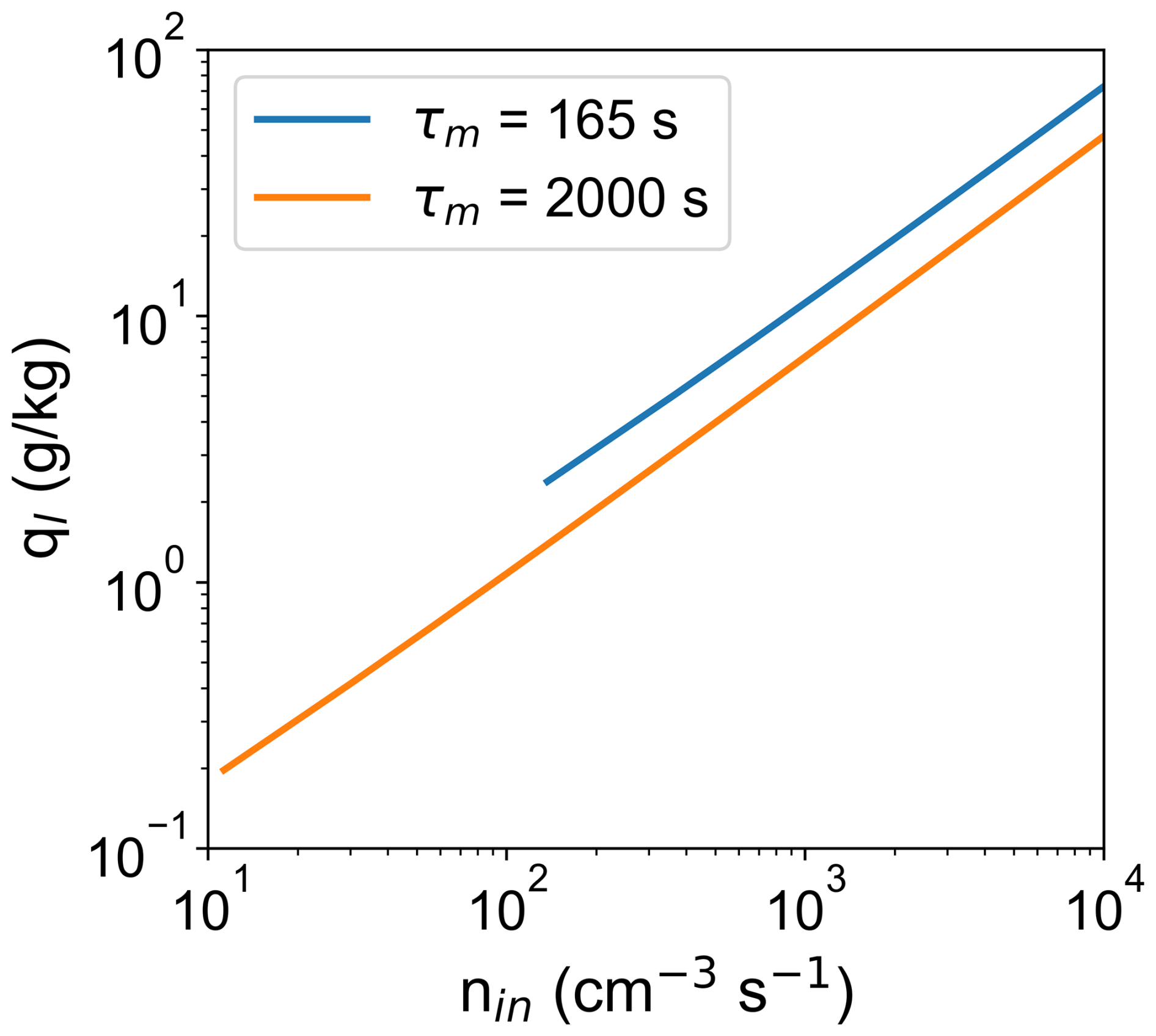
Figure 14 Change of equilibrium liquid water mixing ratio with n_in in the haze-only regime. Results are calculated numerically based on Eqs. (7) to (11), with T₀=290 K and q_v0=13.9 g kg⁻¹. Blue and orange lines are for τ_m=165 and 2000 s, respectively. The left ends of the two lines are determined at RH =100 %.

For a given forcing (T₀, q_v0, and τ_m) and aerosol (r_dry) condition, we can calculate the equilibrium liquid water mixing ratio at the haze-only steady state by solving Eqs. (7)–(11) numerically. For a direct comparison with the above results, we set T₀=290 K, q_v0=13.9 g kg⁻¹, and τ_m=165 s, the same as those used in the box model. Figure 14 shows that q_l increases with n_in linearly in log–log space with a slope of about 0.83, which is steeper than that in the fast microphysics regime (0.67). Note that we only simulate the haze-only regime in the subsaturated environment here (i.e., RH <100 %; the left ends of the two lines in Fig. 14 are determined at RH =100 %), and the slope should be related to the RH dependence of r_eq (Eq. 10). Results show that the required n_in to reach this haze-only regime is extremely high, hundreds to thousands of cubic centimeters per second (cm⁻³ s⁻¹), and q_l is also exceptionally high, tens to hundreds of grams per kilogram (g kg⁻¹). The main reason for the high n_in and q_l is that a huge number of slowly sedimenting haze particles are needed to balance the relatively strong forcing term to replenish water vapor so that s<0 all the time. Such high q_l is likely unrealistic and unachievable in the real chamber due to factors not considered in the model (see the following section). However, if τ_m=2000 s, implying a much weaker forcing, q_l in the haze-only regime can be less than 1 g kg⁻¹ for a more realistic n_in (Fig. 14).

So far, we have demonstrated the existence of the haze-only microphysics regime in an idealized scenario. One question is whether the haze-only regime is stable. We expect that the steady state in the haze-only regime is stable for a given n_in. This is because the aerosol injection rate should be equal to the sedimentation rate of haze particles in the steady state (see Eq. 11). If there is a positive (or negative) perturbation of N_h, the sedimentation rate would increase (or decrease), leading to a net decreasing (or increasing) tendency in N_h for a given n_in. This feedback is trying to bring N_h back to its steady-state value. Of course, this is only our conjecture, not a formal proof. Further efforts are needed to understand the onset of oscillation, the transition between the oscillation regime and haze-only regime, and the stability of the haze-only regime.

3.2.6 Impact of a haze sink

So far, the only sink for aerosol particles is activation. At high aerosol injection rates, activation is suppressed, and thus, they can accumulate when using the CL_CCN scheme (see black lines in Figs. 5 and 12, third row). Similarly, the sink for haze particles is dominated by activation because their sedimentation speed is very small. We have shown that a chamber with subsaturated side walls can efficiently transfer cloud droplets to haze particles over time, leading to haze accumulation when using the CL_Haze scheme (red line in Fig. 12, third row). In reality, these unactivated particles (aerosols or haze particles) can also be lost by side walls, coagulation, sedimentation, or droplet scavenging, preventing their concentration from approaching infinity.

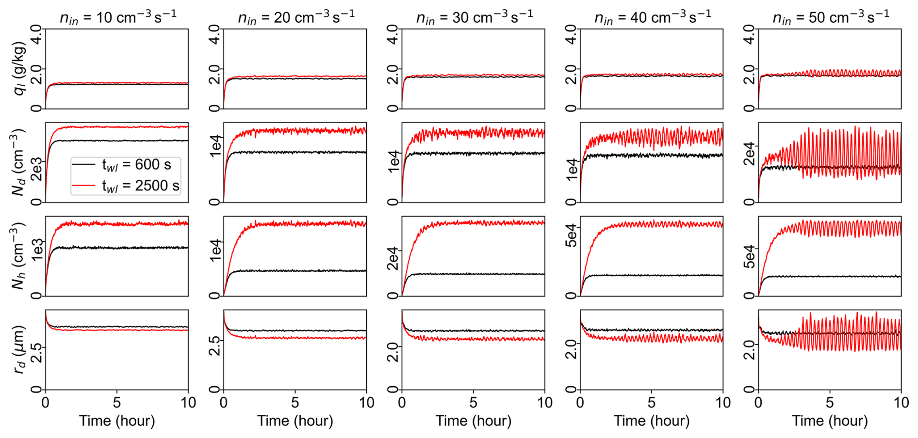
Figure 15 Similar to Fig. 5, time series of domain-averaged q_l (first row), N_d (second row), N_h (third row), and r_d (fourth row) for five different n_in, 10, 20, 30, 40, and 50 cm⁻³ s⁻¹, but considering the loss of haze particles due to the side wall. Different line colors represent simulations using different wall-loss timescales (t_wl in Eq. 12): t_wl=600 s (black) and 2500 s (red).

To investigate the impact of the sink of haze particles on cloud properties, especially in the cloud oscillation regime, following Thomas et al. (2023) and Wang et al. (2024c) (Eq. 1 therein), a wall-loss timescale (t_wl) is applied to constrain N_h when using the CL_Haze scheme as

$$\begin{array}{}\text{(12)}& \mathit{\delta }{N}_{\mathrm{h}}=-N_{\mathrm{h}}{\displaystyle \frac{\mathrm{\Delta }t}{t_{\mathrm{wl}}}}.\end{array}$$

Here Δt is the time step of the simulation, and δN_h is the loss of haze particles due to walls after each time step. t_wl is 1 over the particle rate loss coefficient (β) due to the walls. β can be estimated from the deposition velocity (v_dep) and the ratio of the wall area (A) to volume (V) (for the Pi chamber $A/V=\mathrm{4}$ m⁻¹): $\mathit{\beta }=v_{\mathrm{dep}}A/V$. For simplification (i.e., neglecting the impact of other factors, such as particle size and turbulence, on v_dep), we set $v_{\mathrm{dep}}={\mathrm{10}}^{-\mathrm{4}}$ m s⁻¹, a typical value for the deposition velocity for particles with a diameter of 2 µm (see Fig. 4 in Lai, 2002), which give us $\mathit{\beta }=\mathrm{4}\times {\mathrm{10}}^{-\mathrm{4}}$ s⁻¹ or t_wl=2500 s. Results show that oscillation still exists for n_in≥ 20 cm⁻³ s⁻¹ but with a smaller amplitude (red line in Fig. 15). The oscillation frequency is also higher than before (compare Figs. 5 and 15 for the same n_in). Although we only consider the loss of haze particles due to walls here, there are some other types of haze sinks, such as Brownian coagulation (Baker and Charlson, 1990) and scavenging (Sellegri et al., 2003), which might lead to a smaller effective t_wl in the real chamber. For another sensitivity test, we set t_wl=600 s, the same value Thomas et al. (2019) used to constrain particle concentration for the Pi chamber simulation. Results show that the oscillation is barely seen (black line in Fig. 15). Also note that N_h increases with n_in, but its value is 1 order of magnitude smaller than before (Fig. 15 vs. 5, third row). Combined with the “cloud collapse” findings, our results suggest that achieving a high concentration of haze particles and synchronized activation throughout the chamber are two key factors for the cloud to stay in the oscillation regime.

4 Conclusions and discussion

In this study, we conducted a series of large-eddy simulations of the Pi chamber using a haze-capable bin microphysics scheme (CL_Haze) developed by Yang et al. (2023) to explore haze–cloud interactions over a wide range of aerosol injection rates (0.001 cm⁻³ s${}^{-\mathrm{1}}\le n_{\mathrm{in}}\le \mathrm{50}$ cm⁻³ s⁻¹). Results are compared with simulations using a CCN-based bin microphysics scheme (CL_CCN). The CL_CCN scheme adopts a Twomey-type activation parameterization, which is widely used in atmospheric cloud simulations, while the CL_Haze scheme can properly resolve the growth of haze particles and the activation process. Our objectives were to investigate (1) the influence of different aerosol injection rates on cloud properties and (2) the importance of haze–cloud interactions in a convection cloud chamber as well as in analogous natural cloud systems. For objective 1, we especially focused on the impact of n_in on cloud droplet number concentration (N_d), liquid water mixing ratio (q_l), and droplet size distribution and compared results with previous analytical studies (Krueger, 2020; Shaw et al., 2023). Objective 2 is motivated by Yang et al. (2023), showing that cloud microphysical properties gained with the CL_CCN scheme are similar to those using the CL_Haze scheme, raising the question of whether we need to consider haze–cloud interactions. However, only two aerosol injection rates were investigated in Yang et al. (2023). Here, we explored the consistency of the CL_CCN scheme and the CL_Haze scheme over a wider range of aerosol injection rates. Low-dimensional models are also employed to explore the impact of n_in on cloud properties. In short, we confirm slow and fast microphysics regimes reported in previous studies (Shaw et al., 2023). We also find new microphysical regimes at high aerosol injection rates, cloud oscillation, and haze only, as illustrated in Fig. 16.

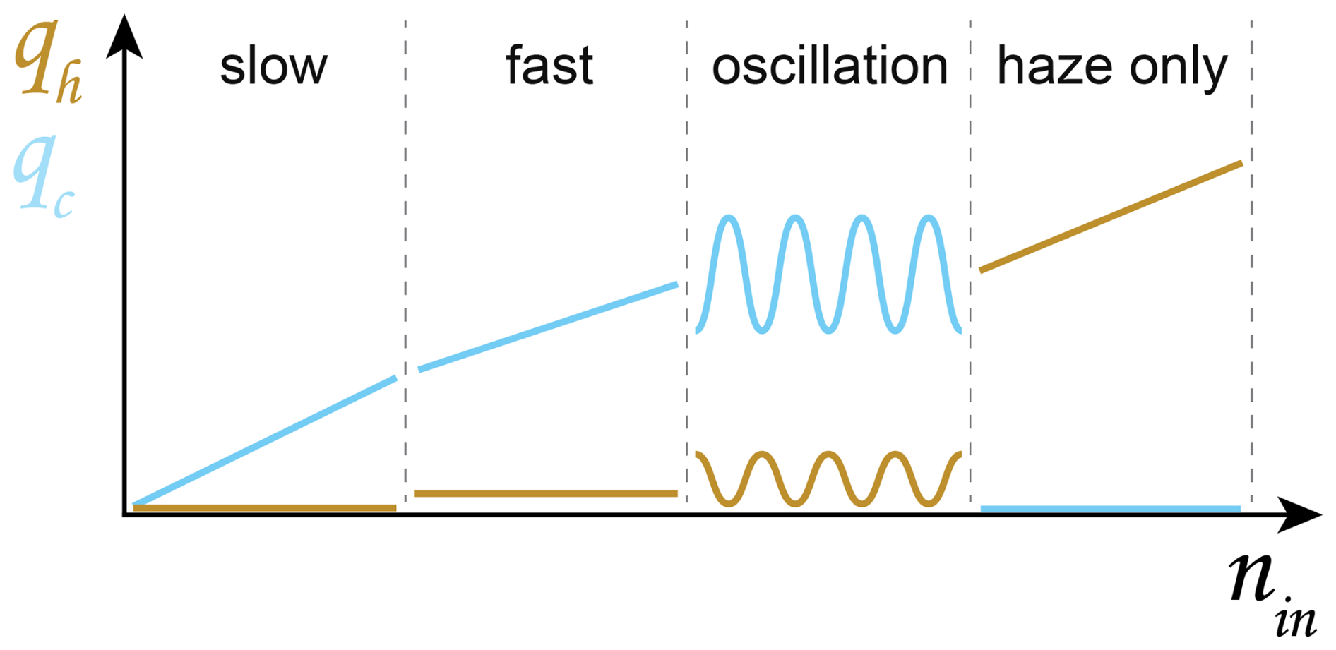
Figure 16 A schematic illustration of q_c or q_h and n_in relationships in different microphysics regimes: slow, fast, oscillation, and haze only.

Slow and fast microphysics regimes were observed at small and moderate aerosol injection rates, respectively. The change of cloud properties with aerosol injection rate in these two regimes agreed with previous analytical studies (Chandrakar et al., 2020; Shaw et al., 2023). Specifically, for small aerosol injection rates (n_in<0.1 cm⁻³ s⁻¹), the cloud was in the slow microphysics regime where droplets grow at a high supersaturation before they fall out, leading to a linear relationship between N_d and n_in as well as q_l and n_in. For moderate aerosol injection rates (0.1 cm⁻³ s${}^{-\mathrm{1}}\le n_{\mathrm{in}}\le \mathrm{10}$ cm⁻³ s⁻¹), the cloud was in the fast microphysics regime with $N_{\mathrm{d}}\sim n_{\mathrm{in}}^{\mathrm{5}/\mathrm{3}}$ and $q_{\mathrm{l}}\sim n_{\mathrm{in}}^{\mathrm{2}/\mathrm{3}}$, consistent with the theoretical prediction in Shaw et al. (2023). In addition, droplet size distributions in the steady state became narrower and shifted to smaller sizes due to the increase in n_in, and the shape of the distribution also agreed reasonably well with analytical estimates (Chandrakar et al., 2020; Liu and Hallett, 1998; Krueger, 2020). But those analytical estimates do not capture the distribution properties at large n_in where haze mode is present.

The most striking phenomena are cloud oscillation, cloud collapse, and haze-only regimes that occur at high aerosol injection rates when using the CL_Haze scheme. In contrast, cloud always reaches a steady state when using the CL_CCN scheme. Haze–cloud interactions are responsible for the occurrence of these microphysics regimes. Specifically, in the cloud oscillation regime, s oscillates around s_crit and σ_s≪s_crit. Under this condition, the cloud system is buffered by a huge number of haze particles and cloud droplets. Droplet activation is controlled by the mean supersaturation rather than supersaturation fluctuation. Droplet deactivation can still occur in a supersaturated environment ($\mathrm{0}<s<s_{\mathrm{crit}}$) due to the curvature effect. The oscillation of s around s_crit leads to the oscillation of droplet activation and deactivation and further causes the oscillation of cloud properties. In a chamber with relatively humid side walls, the supersaturation is more homogeneous in the chamber, and droplets at different locations experience similar supersaturation, leading to synchronized activation (s>s_crit) of a huge number of droplets across the whole chamber – the main reason for cloud oscillation. In contrast, cloud collapse occurs when the side walls are relatively dry. Under this condition, supersaturation in the chamber is more inhomogeneous: droplets close to the side walls tend to be deactivated to haze particles, while droplets away from the side walls tend to grow. The separation of droplet activation (in regions near the center, top, and bottom surfaces) and deactivation (in regions near the side walls) make the chamber an efficient machine to transfer cloud droplets to haze particles – the fundamental reason for cloud collapse. The haze-only regime occurred at extremely high aerosol injection rates. In this regime, s is much smaller than s_crit, and it can be negative (corresponding to RH <100 %). Droplet activation is suppressed, and the formation of haze particles is balanced by their loss due to sedimentation.

In the real chamber, haze particles can also be removed through other mechanisms, such as wall loss and scavenging, which could constrain the haze number concentration. Therefore, clouds might struggle to achieve oscillation and haze-only regimes, especially when the source term to maintain high supersaturation is strong, e.g., a large temperature difference between top and bottom surfaces, like in this study. Haze–cloud oscillation is more likely to occur under conditions of weak supersaturation forcing, e.g., a small temperature difference between top and bottom surfaces in a convection chamber or small updraft velocity in the real atmosphere. Recently, Gutiérrez et al. (2024) solved coupled equations for droplet growth and supersaturation development in a rising cloud parcel. Their analysis also predicts the oscillation between haze and cloud droplets under certain conditions, e.g., low air vertical velocity and high aerosol number concentration. The fundamental reason for cloud oscillation stems from the nonlinear interactions in the coupled haze–cloud–supersaturation system (Arabas and Shima, 2017). Such a system is analogous to other predator–prey systems observed in nature, which causes similar oscillation behaviors, such as oscillation in open-cellular convection or in aerosol–cloud–precipitation system (Koren and Feingold, 2011). However, it should be mentioned that cloud oscillation reported in Gutiérrez et al. (2024) is not the same as oscillation reported in this study: they only have one size of droplet/haze that varies in time, while we have coexisting haze and cloud droplets.

Our results suggest that haze–cloud interactions are very important when air supersaturation is close to the critical supersaturation of aerosols. This condition happens in the Pi chamber at high aerosol injection rates, as shown in this study, and it can also occur in the atmosphere, for example, when cloud or fog is close to the source of intense natural and anthropogenic aerosol emissions. Studies have shown the possibility of fog consisting of just unactivated haze particles in a highly polluted environment (e.g., Klemm and Lin, 2016). The unactivated haze particles can significantly impact fog optical properties, such as visibility and radiation (Boutle et al., 2018), as well as cloud optical properties, i.e., cloud albedo (Hoffmann et al., 2022). Proper simulation of haze–cloud interactions requires resolving haze particles as well as the associated droplet activation and deactivation processes, rather than relying on Twomey-type activation parameterization. Also note that monodisperse aerosol with a dry radius of 62.5 nm is used in this study. We expect haze–cloud interaction might be more important for larger aerosol particles because their critical supersaturation gets smaller, their equilibrium wet radius gets larger, and the activation/deactivation timescale could get longer (Hoffmann, 2016). In addition, aerosol particles in nature vary in size and composition, and haze–cloud interactions might be more important for polydisperse aerosols (see Fig. 5 in Richter et al., 2021). Furthermore, unlike well-controlled environmental conditions in the cloud chamber, the boundary conditions of natural clouds or fogs change over time, which would also affect the microphysical regimes. The impact of haze–cloud interactions under real cloud conditions is worth exploring in the future.