Measurement report: Can zenith wet delay from GNSS “see” atmospheric turbulence? Insights from case studies across diverse climate zones

Global navigation satellite system (GNSS) microwave signals are nearly unaffected by clouds but are delayed as they travel the troposphere. The hydrostatic delay accounts for approximately 90 % of the total delay and can be modelled well as a function of temperature, pressure, and humidity. On the other hand, the wet delay is highly variable in space and time, making it difficult to model accurately. A zenith wet delay (ZWD) can be estimated as part of the GNSS positioning adjustment and is proportional to the specific humidity in the atmospheric boundary layer (ABL). While its average term can describe mesoscale events, its small-scale component is associated with turbulent processes in the ABL and is the focus of the present contribution. We introduce a new filtering and estimation strategy to analyse small-scale ZWD variations, addressing questions related to daily or periodic variations in some turbulent parameters and to the dependence of these parameters on climate zones. Five GNSS stations were selected for case studies, revealing promising specific daily and seasonal patterns depending on the estimated turbulence at the GNSS station (buoyancy or shear). This research lays the groundwork for more accurate models and prediction strategies for integrated water vapour, WV (and potentially liquid water clouds), turbulence. It has far-reaching applications, from nowcasting uncertainty assessments to the stochastic modelling for very large baseline interferometry or GNSS.

1 Introduction

The atmospheric boundary layer (ABL) reaches from the Earth's surface to about 1–2 km above the ground. This layer experiences rapid atmospheric changes, including cloud formation and convective initiation, as well as intense precipitation events linked to elevated temperatures in the context of climate change (Webb et al., 2016). It is characterized by large sources of water vapour (WV).

Turbulent processes in the ABL trigger the redistribution of trace gases, aerosols, heat, WV, and momentum (Stull, 2003). Understanding the transport of such scalars is crucial across various fields, including meteorology, hydrology (Shawon et al., 2021), agriculture (Curto et al., 2022), and air quality control (Zhou et al., 2022). More specifically, enhancing the characterization of WV and liquid water cloud content at small (turbulent) scales within the ABL will provide new insights, aiding in (i) the evaluation and improvement of turbulence parameterizations in numerical weather prediction (NWP) models for nowcasting (Lee and Meyers, 2023); (ii) the refinement of radiative transfer models (RTMs; Calbet et al., 2018), which simulate the absorption and emission of atmospheric molecular constituents layer by layer and (iii) the mitigation of atmospheric distortions in interferometric synthetic aperture radar (INSAR; Chang and He, 2011) or in very long baseline interferometry (VLBI; Teke et al., 2013b) and global navigation satellite system (GNSS) stochastic description (Kermarrec and Schön, 2014). Thus, microwave signals from high-rate GNSS experience a tropospheric delay, which is estimated in the zenith direction during the positioning adjustment (Hobiger and Jakowski, 2017). This delay is divided into two components: the hydrostatic delay, also called dry delay, and the zenith wet delay (ZWD), the latter being proportional to the specific humidity averaged vertically over the lower atmosphere (Bevis et al., 1992) and, thus, connected to WV content in the ABL. Like electromagnetic-phase measurements defined by the integrated refractivity index (Wheelon, 2001), ZWD can be decomposed into an average and a rapidly fluctuating term. The latter is related to atmospheric WV turbulence and is the topic of our contribution. Potential cumulus clouds may cause delays of several millimetres, thus affecting the small-scale variability in the ZWD. Solheim et al. (1999) stated that a cloud droplet concentration of 1 g m⁻³ over a distance of 1 km results in an integrated liquid value of 1 mm, causing a radio path delay of 1.45 mm. In the following, WV will be understood to mean WV and liquid water clouds.

The spectral content, or power spectral density (psd) of these temporal fluctuations, is usually described by the von Kármán model (Wheelon, 2001). In its simplest form, this model consists of three parameters: (i) the slope or decay of psd at high frequencies, (ii) a cutoff or transition frequency below which the spectrum saturates, and (iii) a variance related to WV turbulence strength. All three quantities can be estimated conjointly using statistical methods. In the spatial domain and using the Taylor frozen hypothesis (Taylor, 1938), the cutoff is called the outer-scale length. This parameter marks the end of the inertial range where isotropy can no longer be assumed (Basu and Holtslag, 2022), making it particularly intriguing. Improved characterization of the cutoff from ZWD will provide new insights into this region of the spectrum and improve the understanding of (integrated) WV turbulence processes in the ABL. Before reaching ambitious goals such as uncertainty modelling in nowcasting, improved stochastic modelling of GNSS observations, or correction of satellite images from the retrieval of the turbulent parameters, the following simple yet challenging questions must first be addressed.

• Which methodology is suitable for filtering turbulent fluctuations and estimating the parameters (cutoff, turbulence strength)?

• Do the retrieved turbulent parameters have daily or periodic variations, which would indicate that they can be used to characterize turbulence?

• Do the strength and cutoff estimated from ZWD fluctuations depend on the climate zone?

By answering these questions, we develop a solid methodology and pave the way for a more detailed study to derive machine learning strategies to predict and study the dependencies of integrated WV turbulence in the zenith direction from GNSS ZWD (see, e.g. Pierzyna et al. (2023) in the optical field for the refractivity index). In this first contribution, we will introduce a new filtering and estimation strategy to extract and analyse the small-scale variations from ZWD time series. We will show how cutoff and strength are related through various case studies. To reach that goal, we have selected five GNSS stations worldwide that correspond to different climates or locations known for local effects, such as gravity waves, wind shear, or the proximity of the ocean. Our aim is not to derive climatological conclusions, which would require years of observations, but rather to demonstrate that specific daily and seasonal patterns can be identified. This serves as a first step toward developing more accurate models and prediction strategies, sparking curiosity about these new parameters.

The remainder of this paper is as follows: in the first section, we will introduce the mathematical background to compute and filter the ZWD and retrieve the turbulent parameters. The second section presents results for the GNSS stations that we chose, which located in different climate zones, for 2 specific days (winter/summer). We conclude with some general considerations and an outlook.

2 Mathematical background: ZWD and its fluctuations

In this section, we introduce how ZWD and ZWD fluctuations can be retrieved from GNSS observations and develop the methodology to estimate the turbulent parameters.

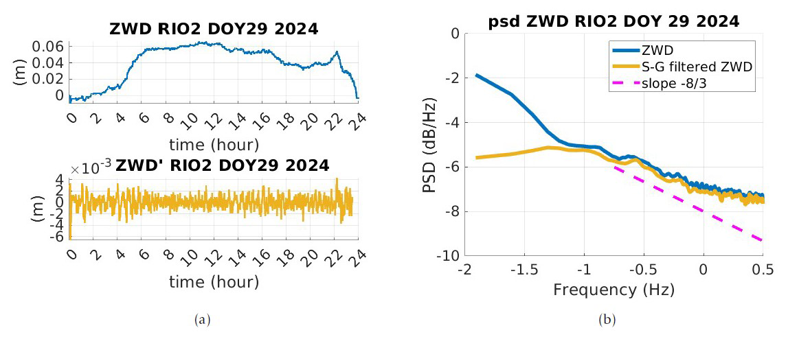
Figure 1 Illustration of the filtering of the ZWD from low-frequency effects related to mesoscale circulation. (a) Top – the original ZWD; bottom – S-G-filtered ZWD corresponding to ZWD^′. Panel (b) shows the corresponding psd of GNSS station RIO2 on DOY 29 (2024).

2.1 Estimation of ZTD and ZWD

Data processing and illustration of the filtering strategy

We estimate the atmospheric zenith total delay (ZTD) from the GNSS observations of the stations described in Sect. 3 using the Earth Parameter and Orbit System (EPOS) GNSS software in precise point positioning mode (Zumberge et al., 1997) at a 30 s rate. The GeoForschungsZentrum (GFZ) satellite orbit and clock used are estimated from a global GNSS network with about 140 stations. The products are not entirely error-free, but the large number of stations gives us confidence that the high-frequency signal caused by turbulence does not affect the satellite orbit and clock products. These two remain very smooth and are suitable for detecting the high-frequency signal observed at a single station. The pressure is obtained from the Generative Pre-trained Transformer 2 (GTP2) model (Lagler et al., 2013). Since daily pressure variations are slow and typically within a few hPa, using constant pressure may introduce a low-frequency error in ZWD but should not affect the detection of turbulence signals. During the estimation, we do not constrain the ZTD to follow a random walk to avoid biasing the spectral content of the fluctuation term of the ZWD toward a specific power law (−2 for a random walk). We thus avoid obscuring the Kolmogorov turbulence spectrum (a power law of $-\mathrm{8}/\mathrm{3}$ corresponding to integrated WV; see Eq. 6 for more details). An example of a ZWD for the station RIO2 on 29 January 2024 is provided in Fig. 1a  top. A significant increase in ZWD is noticeable around 04:00 UTC, highlighting a specific mesoscale circulation for the day under consideration.

We illustrate the principle of the Savitzky–Golay (S-G) filter by plotting the power spectral density (psd) before and after filtering in Fig. 1a and b. As shown in Fig. 1b (yellow line), the low frequencies of ZWD (blue line) are eliminated properly, leading to a time series of fluctuations (ZWD^′) as shown in Fig. 1a  bottom. Its psd corresponds to a von Kármán model (Sect. 2.2.2), with additional white noise identified at a high frequency. For visual analysis, the expected $-\mathrm{8}/\mathrm{3}$ slope is plotted as a dotted magenta line in Fig. 1b.

Atmospheric WV is responsible for the propagation delay experienced by GNSS signals, called the slant wet delay and commonly defined as the integral of the wet refractivity along the slant path above the station (Bevis et al., 1992). Through GNSS positioning adjustment, the ZTD can be estimated, which is decomposed into (i) a hydrostatic term and (ii) a term accounting for the wet delay, called ZWD. The hydrostatic delay is effectively modelled using, for instance, the Saastamoinen approach (Saastamoinen, 1972) and is about 80 %–90 % of the ZTD (Tregoning and Herring, 2006). The ZWD is proportional to the specific humidity q averaged in the vertical direction over the depth of the lower-atmosphere H where WV is concentrated. It is expressed as

$$\begin{array}{}\text{(1)}& \mathrm{ZWD}={\displaystyle \frac{\mathrm{1}}{{\mathit{\kappa }}^{\prime }}}\underset{\mathrm{0}}{\overset{H}{\int }}\mathit{\rho }q\mathrm{d}z,\end{array}$$

with κ^′ indicating a factor depending on the surface temperature and specific gas constant (Bevis et al., 1992). Please note that this formula is only an approximation.

2.2 ZWD fluctuations

Similarly to atmospheric temperature, pressure, or wind (Wheelon, 2001), ZWD can be divided into two components expressed as

$$\begin{array}{}\text{(2)}& \mathrm{ZWD}=\langle \mathrm{ZWD}\rangle +{\mathrm{ZWD}}^{\prime },\end{array}$$

where (i) 〈ZWD〉 describes mesoscale changes in the ambient value, such as gradual diurnal or seasonal variations or sudden changes associated with weather fronts passing (Bevis et al., 1992), and (ii) ZWD^′ is a random component corresponding to turbulent fluctuations. This random component should be filtered from the estimated ZWD to enable a deeper study of its spectral content. Developing a proper methodology to achieve this goal is the central focus of this contribution.

Please note that for the analysis, we used ZWD corrections to the a priori constant ZWD, allowing negative values to be plotted. For simplicity, these corrections are referred to as ZWD and represent adjustments to the ZTD. These were used to derive the turbulence parameters. The slow variations (low frequencies related to periods longer than 30 min) of zenith hydrostatic delay (ZHD) and ZWD will not impact our results.

2.2.1 Extracting the ZWD fluctuations

To study the ZWD fluctuations only, we filter ZWD^′ from the ZWD time series using the Savitzky–Golay (S-G) filter (Savitzky and Golay, 1964) with a Kaiser window weighting to limit boundary effects (Schmid et al., 2022). S-G filters are commonly used to smooth out noisy signals that have a broad frequency range. Also known as digital smoothing polynomial filters or least-squares smoothing filters, the S-G filters often outperform standard averaging finite impulse response filters by preserving high-frequency content – here the ZWD^′. This is the main reason why we have chosen this approach, the same as in Kermarrec et al. (2023), besides its simplicity of use.

Choice of the filter parameters

The S-G filter uses the least-squares fit of a small set of consecutive data points to a polynomial. In each iteration, the central point of the fitted polynomial curve becomes the new smoothed data point. We assume that the integrated WV fluctuations in the ABL are stationary for about 30 min–1 h, so the term 〈ZWD〉 should contain frequencies that are smaller than $\mathrm{1}/\mathrm{3600}$ = 2.7 × 10⁻⁴ Hz. These latter correspond to mesoscale effects and should be filtered from the ZWD. To achieve the desired low-pass filtering effect at this specific cutoff frequency, two parameters must be adjusted: (i) the polynomial order d, typically set to 3 to prevent overfitting, and (ii) the half-width of the smoothing window m. A large value of m will produce a very smooth filtered time series 〈ZWD〉. Following Schafer (2011), we fix m based on the 3 dB cutoff frequency fc, which is given empirically by

$$\begin{array}{}\text{(3)}& \mathrm{fc}={\displaystyle \frac{d+\mathrm{1}}{\mathrm{3.2}m-\mathrm{4.6}}}.\end{array}$$

From physical considerations, the spectrum of ZWD^′ is expected to saturate at a cutoff frequency α between 0.1 and 0.005 Hz, which corresponds approximately to an outer-scale length of turbulence between 80 and 2000 m in the ABL, assuming a geostrophic wind velocity of 8 m s⁻¹ and that the Taylor frozen hypothesis holds, as described in Sect. 2.3 (Ziad, 2016). Thus, the S-G filter should remove frequencies slightly below α to ensure that only the low frequencies corresponding to 〈ZWD〉 are eliminated. We found this balance by setting m=300 to select frequencies with a period slightly above 1 h for observations at a data rate of 30 s. This way, we can expect that the spectrum of ZWD^′ will saturate, and the mesoscale effects of 〈ZWD〉 are eliminated. If this is not the case, implausibly small values of α will arise, be considered outliers, and be excluded from our analysis. Possible causes are related to the data themselves (outliers, small jumps, gaps) or turbulence effects (anisotropy, violation of the Kolmogorov assumption). A sensitivity analysis on m has shown that values varying m in the range of [220,350] did not affect the estimated parameters more than 5 %, which is statistically negligible and will not affect our conclusions.

The filter requires adjustment near sample boundaries when the window extends beyond the input vector. We use a Kaiser window to weight the time series as proposed in Schmid et al. (2022), with a value of 3 found optimal for ZWD.

2.2.2 The spectrum of the ZWD fluctuations

Turbulent flow can be viewed as a collection of swirling motions called eddies or vortices. According to Kolmogorov, energy is transferred sequentially from larger to smaller eddies at a constant rate, a process known as the turbulent energy cascade, which describes 3D isotropic turbulence (Stull, 2003). The ABL flows vary significantly based on the interaction between wind shear and buoyancy forces. Shear instabilities occur locally, while buoyancy forces create vigorous thermals that transport heat and momentum over larger distances. These forces can also work together to modify the flow dynamics within the ABL (Moeng and Sullivan, 1994).

In turbulence theory, the (spatial) power spectrum represents the distribution of kinetic energy of these eddies across various length scales. The inertial range of the spectrum corresponds to the length scales over which energy transfer occurs, with negligible dissipation due to molecular viscosity. The $-\mathrm{5}/\mathrm{3}$ power law of the energy spectrum can be derived from dimensional analysis and holds within the inertial range. In this region, Tatarski (Tatarski et al., 1961) proposed a Kolmogorov wave number spectrum (1D) for scalar quantities such as temperature or humidity as follows:

$$\begin{array}{}\text{(4)}& {\mathrm{\Phi }}_x\left(k\right)=C_x{k}^{-\mathrm{5}/\mathrm{3}},\end{array}$$

where Φ_x is the power spectrum of the scalar quantity x, k is the wave number, and C_x is a constant related to the structure of the turbulent field.

The von Kármán spectrum is mathematically more convenient, as it avoids an infinite growth of the variance at large scales and is physically tractable (Wheelon, 2001). It is given in its simplest form by

$$\begin{array}{}\text{(5)}& V_x\left(\mathit{\kappa }\right)\propto C_x^{\mathrm{2}}{\left({\mathit{\kappa }}^{\mathrm{2}}+{\mathit{\kappa }}_{\mathrm{0}}^{\mathrm{2}}\right)}^{-\mathrm{5}/\mathrm{6}}\end{array}$$

and still has the typical $-\mathrm{5}/\mathrm{3}$ slope for the 1D case. The von Kármán spectrum saturates for small κ below the outer-scale length L₀ defined as ${\mathit{\kappa }}_{\mathrm{0}}=\mathrm{2}\mathit{\pi }/L_{\mathrm{0}}$.

These formulas are valid for scalars such as humidity and temperature but have to be adapted for integrated scalars such as phase or ZWD. Since ZWD is a time series of integrated WV, we will now focus on deriving the temporal spectrum.

2.3 Taylor's frozen hypothesis

Despite the wind's stochastic nature over time and space, a temporal power spectrum can be derived from Eq. (5) under the Taylor frozen hypothesis (Taylor, 1938). This hypothesis assumes that the medium remains static between measurements, with time translated into distance scaled by the velocity of turbulent irregularities.

Phase measurements of electromagnetic signals are proportional to the integrated refractivity index along the propagation path. The temporal power spectrum for the phase fluctuations can be derived using the von Kármán model, and, by analogy, the power spectrum for integrated WV can be expressed as

$$\begin{array}{}\text{(6)}& W_{\text{intWV}}\left(\mathit{\omega }\right)\propto {\displaystyle \frac{C_{\text{intWV}}^{\mathrm{2}}{v}^{\mathrm{5}/\mathrm{3}}}{{\left({\mathit{\omega }}^{\mathrm{2}}+{\mathit{\kappa }}_{\mathrm{0}}^{\mathrm{2}}{v}^{\mathrm{2}}\right)}^{\mathrm{5}/\mathrm{6}+\mathrm{1}/\mathrm{2}}}}={\displaystyle \frac{C_{\text{intWV}}^{\mathrm{2}}{v}^{\mathrm{5}/\mathrm{3}}}{{\left({\mathit{\omega }}^{\mathrm{2}}+{\mathit{\kappa }}_{\mathrm{0}}^{\mathrm{2}}{v}^{\mathrm{2}}\right)}^{\mathrm{4}/\mathrm{3}}}},\end{array}$$

with v the wind velocity in the top part of the boundary layer (geostrophic wind), $C_{\text{intWV}}^{\mathrm{2}}$ the structure constant of the integrated WV, and ${\mathit{\kappa }}_{\mathrm{0}}=\mathrm{2}\mathit{\pi }v/L_{\mathrm{0}}$. The spectrum exhibits a $-\mathrm{8}/\mathrm{3}$ slope and saturates at a cutoff frequency κ₀v; see Wheelon (2001) or Ishimaru (2005) (in Appendix B).

The temporal spectrum W_intWV corresponds to a Matérn spectrum in statistics (Lilly et al., 2017) and can be parameterized in a simplified form as

$$\begin{array}{}\text{(7)}& W_x\left(\mathit{\omega }\right)={\displaystyle \frac{{\mathit{\sigma }}^{\mathrm{2}}{\mathit{\alpha }}^{\mathrm{5}/\mathrm{3}}}{c_{\mathit{\alpha }}{\left({\mathit{\omega }}^{\mathrm{2}}+{\mathit{\alpha }}^{\mathrm{2}}\right)}^{\mathit{\lambda }}}},\end{array}$$

with $c_{\mathit{\alpha }}=\frac{\mathrm{1}}{\mathrm{2}/\mathit{\pi }}\frac{\mathrm{\Gamma }\left(\mathrm{0.5}\right)\mathrm{\Gamma }(\mathit{\lambda }-\mathrm{0.5})}{\mathrm{\Gamma }\left(\mathit{\lambda }\right)}$. This spectrum is described by three parameters: the variance σ², the slope λ, and α. The parameterization in Eq. (7) proves to be more convenient for numerical optimization during parameter fitting. The growth induced by turbulence is represented by the forcing parameter λ. To counteract this growth, a damping parameter called a cutoff frequency (α) is introduced. According to Kolmogorov theory, the slope is fixed at $\mathit{\lambda }=\mathrm{4}/\mathrm{3}$, as in Eq. (6), leaving two parameters to estimate: α and σ², which are related to the strength of the WV turbulence within the ABL.

Clearly, the Taylor frozen approximation may come to its limit for 30 s rate observations, as were used in this paper. Further, ZWD corresponds to mapped slant delay in the vertical, i.e. a sort of WV mean in a cone dependent on the cutoff chosen for processing the observations. The strong agreement between the theoretical model and the estimated values gives us confidence in the validity of this approximation. For further discussion, see Wheelon (2001, Chap. 6). Using slant delays could be an alternative, but this would result in short, highly noisy time series, complicating the estimation process. Another option might be to reduce the temporal resolution to 1 s, but not all stations are equipped for this, and additional white noise may be introduced and filtered accordingly. We account for these limitations in our interpretation.

We further draw the reader's attention to the fact that the results described in the next section were able to be validated using instruments such as radiometers at stations combining GNSS and VLBI (very long baseline interferometry) (Teke et al., 2013a). However, the interpretation remains uncertain, as they do not sense the same quantity as in the case of GNSS. We leave these investigations for a future publication, using machine learning strategies to search for dependencies.

2.4 Parameter estimation

The estimation of the two turbulence parameters mentioned in Sect. 2.3 from the empirical spectrum of observations often involves iterative regressions, as described in van Dinther and Hartogensis (2014). We propose an alternative method based on the theoretical understanding that the spectrum reflects a Matérn process, as detailed in Eq. (7); see also Lilly et al. (2017) or Kermarrec and Schön (2020). The parameters α and σ² can be estimated using a debiased version of the weighted maximum likelihood estimator (WMLE) (Sykulski et al., 2019). This method is highly effective for small sample sizes and, thus, advantageous, given that stationarity for ZWD^′ should be maintained for only 30 min to 1 h (equivalent to 120 samples at a 30 s data rate).

We have used an improved version of the algorithm to account for additional white noise by joint estimation (Montillet and Bos, 2020). We refer to Sykulski et al. (2019) for more details on the method. Because of the pre-filtering of the ZWD from mesoscale effects, the estimation of a random walk (slope of −2) is not mandatory, which avoids a non-unique minimum in the estimation procedure.

As previously mentioned, the cutoff frequency α and the variance of the process σ² are estimated by fixing the slope to $-\mathrm{8}/\mathrm{3}$ in the WMLE. We further force α to be between 0.005 and 0.1 Hz based on the physical considerations mentioned in Sect. 2.3 and given a wind velocity around 8 m s⁻¹ (Ziad, 2016).

In Cheinet and Cumin (2011), temperature fluctuations (and similarly for the scalar WV) were shown to be log normally distributed, so we can expect a normal distribution for the ZWD, which is favourable for the estimation strategy using MLE. We detect cases where our approach may fail (data gaps, outliers, non-stationarity, violation of the Taylor hypothesis) by computing the degree of error fit (error_fit) between the natural log of the periodogram and that of the fitted spectrum, more specifically the mean squared error between the two quantities. We filter such batches with a threshold-based outlier detection method for which values of error_fit exceeding 3 standard deviations from the mean are excluded. Additionally, we ensure that α stays below 0.005 Hz due to physical considerations and use a similar outlier detection method as the one that is used for error_fit.

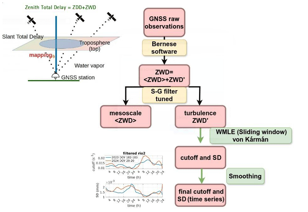
Figure 2 Flowchart summarizing the methodology from the processing of raw GNSS observations to the time series of turbulent parameters α and σ. The small figures are for illustration purposes only.

2.5 Summary of the methodology

Our methodology is summarized in Fig. 2 and in text form in the following.

1. The processing of the GNSS raw observations using, e.g. Bernese or EPOS software, leads to the estimation of the ZWD.

2. The time series are filtered with the S-G filter to extract ZWD^′ only.

3. The parameters α and σ² are estimated batch-wise from the filtered ZWD^′ time series. To that end, we select a window of length LE corresponding to 1 h of observations (LE = 120 epochs for a data rate of 30 s). In the second step, we let the window slide over the data and compute the parameters every 5 epochs (2.5 min for the given data rate). We obtain a time series of values from which we eliminate outliers by setting the lower limit to 3 standard deviations below the mean and the upper limit to 3 standard deviations above the mean. Outliers are replaced by linear interpolation of neighbouring, non-outlier values.

4. In the last step, the time series of parameters α and σ² that we obtained are smoothed using a moving average filter to ease interpretation and pattern recognition (periodicity, variations).

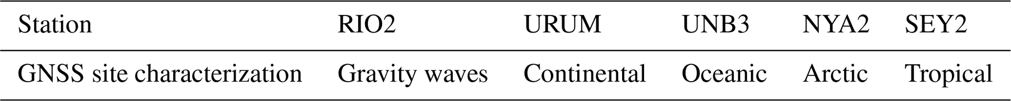
Table 1 Selected GNSS stations and their corresponding climates.

3 Data and results

3.1 GNSS observations

The five GNSS stations selected are located across the globe. To address the questions posed in the introduction, we have chosen stations from the International GNSS Service (IGS) located in different climate zones. At this stage and for this initial contribution to the topic, we aim to showcase the potential of our approach by offering new insights into atmospheric turbulence. The following stations were chosen, as illustrated in Fig. 3, and the corresponding climates are summarized in Table 1. We used all the GNSS satellites from the GFZ multi-GNSS products (GPS, GLONASS, Galileo, BeiDou, and QZSS). In the GNSS data processing, we used the GeoForschungs Zentrum multi-GNSS satellites orbit and clock products in precise point positioning (PPP) mode. Thus, the error in the satellite orbit and clock can be ignored in this study. The 30 s rate ZWDs are estimated in two steps: (i) firstly, the GNSS data are processed in PPP mode with standard parameter settings of ambiguities, 1 h ZWD (with a random walk constraint), 24 h station coordinates, 24 h gradients, and 30 s rate receiver clock error. Turbulence effects were partly absorbed by the estimated 30 s receiver clock parameters, but the majority remained in the observation residuals. Outliers are removed using the 3 times the interquartile range rule. After the first step, we get clean GNSS observations and well-estimated parameters. (ii) In the second step, the estimated parameter corrections (ambiguities, station coordinates, and gradients) from the first step are fixed. The 30 s ZWD and receiver clock are, thus, estimated from the clean GNSS observations, with their initial values also from the first step. We further mention that tropospheric effects were modelled using the VMF1 function (Boehm et al., 2006), that IERS2010 conventions were applied to remove solid Earth and pole tides, and that the FES2004 tidal model was used to model ocean tide loading. The antenna centre-phase variations are corrected using the absolute antenna calibrations in the IGS20 frame during the GNSS data processing. Further, our strategy to analyse the turbulent parameters using the WMLE by fixing the slope should eliminate potential additional effects (non-tidal loading, multipath, or antenna centre-phase variations) if they were present in the ZWD. The ZWD is estimated as an independent delay but is still correlated with the up (also called height) component in the estimation.

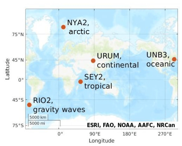
Figure 3 World map illustrating the location of the selected IGS stations with the corresponding climate or specificity.

For each station, we have selected 2 d of observations: one in winter (29 January 2024, date of the year (DOY) 29) and one in summer (1 July 2023, DOY 182), with winter and summer referring to the Northern Hemisphere. We thus cover a broad range of GNSS stations by taking measurements from very different climate zones and seasonal periods. While general conclusions or predictions with machine learning may require processing more days of observations, the days selected enable the identification of patterns. We have further analysed 1 subsequent day (183) that supported our conclusions. It is not shown for the sake of shortness and readability but is provided in Kermarrec and Deng (2024).

For the analysis, please recall that the term ZWD is used for ZWD corrections and represents adjustments to the ZTD. The 24 h GNSS observations are used to estimate the 30 s ZWD. Since the ZWD is highly correlated with other estimated parameters (such as coordinates and clock error), boundary effects can be observed in the estimated ZWD. A sliding window analysis could be considered to mitigate these boundary errors, but it is beyond the scope of our paper and will be addressed in future work. We have accounted for this fact in the processing to compute our parameters by excluding the first batches.

We present the time series of ZWD, α, and σ as well as the $\frac{{\mathit{\sigma }}^{\mathrm{2}}}{\mathit{\alpha }}$ ratio for the 2 d under consideration. The ratio should help identify whether the two estimated parameters have a linear dependency and have their minimum/maximum in phase. Such a dependency would ease prediction with machine learning as well as aid in the establishment of local (i.e. station-related) models. WV turbulence may be affected by mesoscale effects, so ZWD plots are included for completeness. We acknowledge that analysing only 2 d does not allow for general conclusions, but it highlights strong differences and patterns. One should keep in mind that turbulence is local and highly variable, but we analysed daily variations in the new parameters in batch processing (no instantaneous values).

3.2 Climate zones

3.2.1 Continental climate: URUM

The station URUM is located in Ürümqi (China). The city is situated in northwest China, near 44° N, at an altitude ranging from 600 to 1000 m. The climate of Ürümqi is arid continental, featuring freezing winters and hot summers. The nearby mountains make precipitation more frequent in Ürümqi than in other parts of the region, with generally light but frequent snowfalls in winter. In summer, occasional rain occurs, but hydrostatic periods can bring heat waves, with high temperatures reaching 38–40 °C.

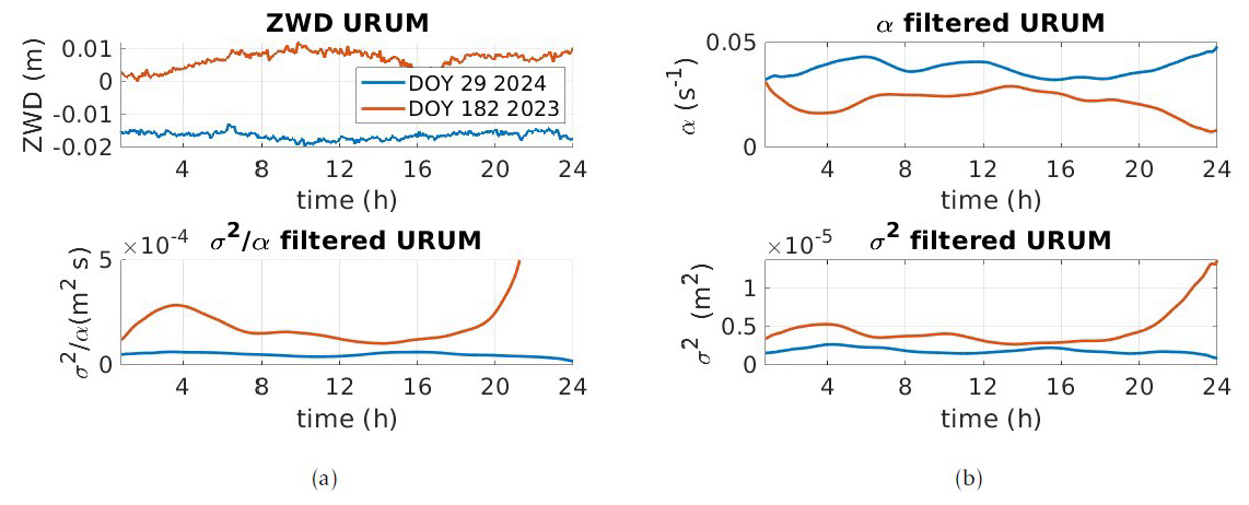
Figure 4 Station URUM (continental climate) (a) top – ZWD (m) for DOY 29 (2024) and DOY 182 (2023); bottom – the ${\mathit{\sigma }}^{\mathrm{2}}/\mathit{\alpha }$ ratio. For panel (b), the top is the cutoff frequency α and the bottom the variance σ². For readability, we have subtracted 0.04 from the ZWD on DOY 29. ZWD is used here to mean ZWD corrections.

Figure 4a  top shows the ZWD for the 2 d under consideration (winter as a blue and summer as a red line). No strong variations are recorded except for the summer day, where a local minimum can be seen around 16:00 UTC, with the decrease starting around approximately 13:00 UTC. A similar decrease in the cutoff frequency α can be identified in Fig. 4b  top. The increase in σ² starts at a slower pace than that in α, as illustrated in Fig. 4a  bottom, with the time-dependent ${\mathit{\sigma }}^{\mathrm{2}}/\mathit{\alpha }$ ratio (red line, positive slope). Interestingly, after the minimum around 16:00 UTC, ZWD increases again, but none of the turbulent parameters are affected by this change. It seems even that the drop in ZWD triggered an increase in the turbulence strength far after the minimum occurred. We note that α has a minimum at 04:00 UTC at night, corresponding to a maximum of σ². However, the ratio is not constant and, thus, does not allow us to derive the proportionality relationship between the two parameters.

In winter, the turbulence strength σ² is smaller than in summer, and so α is correspondingly higher (blue line). The variations are less pronounced than in summer, making us think that the atmosphere may be more stratified and stable. Daily variations are not evident for the day under consideration, and the ${\mathit{\sigma }}^{\mathrm{2}}/\mathit{\alpha }$ ratio is nearly constant, which is favourable for estimation.

3.2.2 Oceanic climate: UNB3

The IGS station UNB3 is one of several continuously operating GNSS reference stations in and near the province of New Brunswick, Canada. It is located in the city of Fredericton. The receiver is part of SuomiNet, a network of GNSS receivers at universities and other locations that provide real-time atmospheric precipitable WV measurements and other geodetic and meteorological information. The station was used in combination with GLONASS to monitor the ionosphere (Banville and Langley, 2015).

The climate at UNB3 is more coastal and maritime than in the inland area of New Brunswick. Moist Atlantic air brings mild winter spells and cool summer periods.

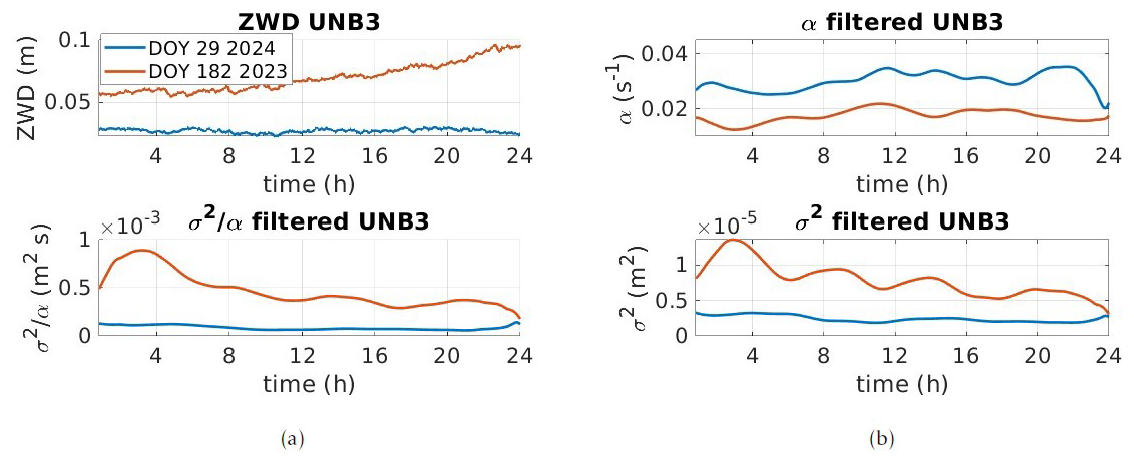
Figure 5 Station UNB3 (oceanic climate) (a) top – ZWD (m) for DOY 29 (2024) and DOY 182 (2023); bottom – the ${\mathit{\sigma }}^{\mathrm{2}}/\mathit{\alpha }$ ratio. For panel (b), the top is the cutoff frequency α and the bottom the variance σ². ZWD is used here to mean ZWD corrections.

From Fig. 5a  top, there is no evidence for strong changes in the WV content. A slow ZWD increase is visible for the summer day starting around 08:00 UTC, which is in parallel with a decrease in turbulence strength; see Fig. 5b  bottom (red line). The variations in α are similar, although the variations are smaller than 0.01 Hz. This finding could be interpreted as the isotropic turbulence becoming less intense, but the corresponding length of the Kolmogorov bandwidth (inertial range) stays (nearly) constant over time (i.e. increasing less intensely than σ² decreases). This leads to a ${\mathit{\sigma }}^{\mathrm{2}}/\mathit{\alpha }$ ratio that decreases linearly instead of remaining constant, so no simple proportionality constant can be deduced for the winter case. A possible interpretation is that the integrated WV increase has damped isotropic turbulence to the benefit of the more elongated structures. We note an evident periodic variation in the turbulent parameters in summer; see Fig. 5b with a period of around 4 h. This pattern could be linked to specific daily mass movement but necessitates further investigation based on additional sensors.

In winter (blue line), on the contrary, the turbulent parameters are less variable. σ² indicates a less intense turbulence strength than in summer. The periodic variations still exist but are less visible. The ${\mathit{\sigma }}^{\mathrm{2}}/\mathit{\alpha }$ ratio is nearly constant with time, the same as for URUM.

Further, the mean value of α is smaller than that of the continental case, which could be attributed to an increase in turbulence strength. In summer, σ² is more than 2 times higher than in winter for the day under consideration. σ² decreases during this particular day in summer, so the heating of the surface, generating convective turbulence, cannot be responsible for turbulence strength only. Additional investigation based on, e.g. the wind velocity, would ease interpretation. The low value of α in summer makes us think that the turbulence should be mostly isotropic (i.e. corresponding to a longer inertial range).

3.2.3 Arctic climate: NYA2

Ny-Ålesund (NYA2 station), located on a fjord on Svalbard's west coast, is influenced by warm ocean currents from lower latitudes that affect the local climate. Despite its high-Arctic location (78.9° N, 11.9° E), summer temperatures remain above freezing, and winter temperatures rarely drop below −25 °C, although they vary significantly from year to year (Maturilli et al., 2013). Männel et al. (2021) validated GNSS-based WV estimation with radiosonde data for 15 months of observations and was able to identify warm-air-intrusion events. At the midlatitudes, the boundary layer is typically one or a few kilometres deep, but in the Arctic, it is much shallower, usually a few hundred metres or less. This is due to the stable stratification caused by the increase in absolute temperature within the lowest kilometre (Mauritsen, 2007). Graßl et al. (2022) analysed high-resolution wind lidar data and found that the atmosphere from 400 to 1000 m above Ny-Ålesund was characterized by a turbulent wind shear zone, linking the micrometeorology of the ABL with the synoptic flow.

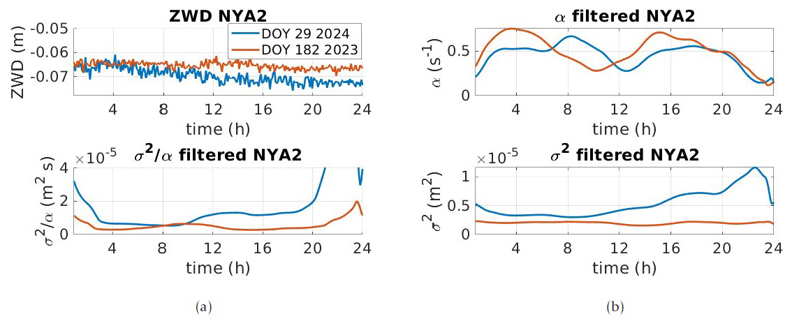
Figure 6 Station NYA2 (arctic climate) (a) top – ZWD (m) for DOY 29 (2024) and DOY 182 (2023); bottom – the ${\mathit{\sigma }}^{\mathrm{2}}/\mathit{\alpha }$ ratio. For panel (b), the top is the cutoff frequency α and the bottom the variance σ². For the sake of readability, we have subtracted 0.1 from ZWD on DOY 182. ZWD is used here to mean ZWD corrections.

From Fig. 6a  top, a slight decrease in ZWD is visible for the winter day (blue line), but there are no strong variations for the summer day (red line). Interestingly, the decrease on DOY 29 (2024) is linked to an increase in the strength of turbulence σ². At UNB3, a ZWD increase and a σ² decrease were observed; for NYA2, there is a ZWD decrease and a σ² increase (Fig. 5b). We further note that σ² is smaller in summer than in winter, which we attribute to more stable and stratified air. The values of α are similar for the days under consideration but vary strongly during the day, with an amplitude of more than 0.2 Hz; see Fig. 6b  top. We identify an increase in α at night, with a maximum at 04:00 and 16:00 UTC in summer and a minimum at 10:00 UTC and at midnight in winter. These maxima are delayed by about 2 h in winter but still exhibit a period of approximately 4 h. This finding could be linked to specific momentum (wind shear) above the station under consideration. We note that the ${\mathit{\sigma }}^{\mathrm{2}}/\mathit{\alpha }$ ratio is not constant, particularly at night. However, in summer, its variations are small in comparison to those in winter. The high value of α combined with low values of σ² can be interpreted as stratified and stable air, which is supported by the aforementioned studies.

The comparison between NYA2 and UNB3 shows that the turbulent parameters cannot be deduced by visual analysis of the ZWD; Their behaviour cannot be predicted without a statistical estimation. Plausible explanations can be deduced from physical considerations that depend on the climate or local conditions at the GNSS station.

3.2.4 RIO2: Tierra del Fuego

Tierra del Fuego (RIO2 station) is located at the southern extremity of South America. The climate is consistently cooler in summer and colder in winter, with significant contrasts in annual rainfall. This area is known as the world's gravity wave hotspot. Strong tropospheric winds create mountain waves year-round. In austral winter, the polar night jet's westerlies allow these waves to penetrate deep into the middle atmosphere, where they deposit momentum and slow the stratospheric flow (Kaifler et al., 2020). Gravity waves in the Earth's atmosphere play a crucial role in the geophysical system, facilitating the transfer of energy and momentum across different scales and connecting various atmospheric layers (Wright et al., 2016). We further mention that RIO2 is located near the sea.

During the 2 d, DOY 29 (2024) and DOY 182 (2023) no strong gravity waves directly above the station could be visually identified at https://worldview.earthdata.nasa.gov/ (last access: 5 January 2025).

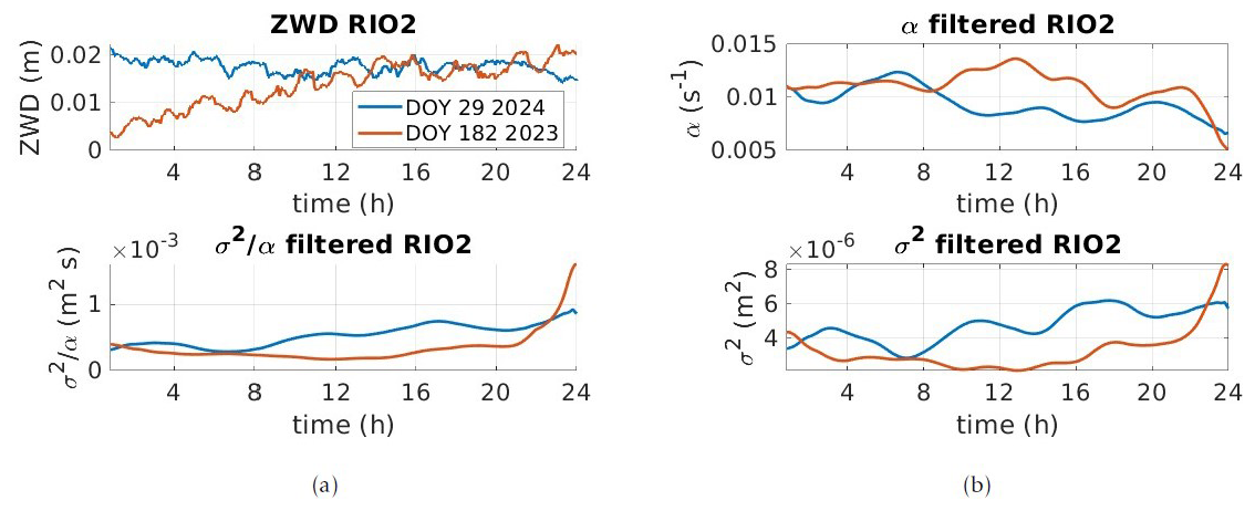
Figure 7 Station RIO2 (tundra, gravity waves) (a) top – ZWD (m) for DOY 29 (2024) and DOY 182 (2023); bottom – the ${\mathit{\sigma }}^{\mathrm{2}}/\mathit{\alpha }$ ratio. For panel (b), the top is the cutoff frequency α and the bottom the variance σ². ZWD is used here to mean ZWD corrections.

In Fig. 7a  top, a clear increase in ZWD is visible from 00:00 to 12:00 UTC in winter (red line in that hemisphere). This increase is followed by a plateau from 13:00 UTC when σ² starts its increase. Thus, the turbulence strength is triggered by the variations but does not occur exactly during the integrated WV increase. In winter, we note that σ² slightly increases during the day but stays at a low level (a factor of 10 lower than for the other stations under consideration; Fig. 7b  bottom, blue line). The parameter α is small, which we will link to a very long inertial range and rather isotropic and well-developed turbulence, most probably due to buoyancy. No strong difference can be identified between summer and winter; i.e. the blue and red curves follow each other. A periodic pattern can be identified, and the time between a maxima and a minima is around 02:00 UTC, thus much smaller than for the station NYA2. This finding supports our interpretation that a different type of turbulence occurs, potentially linked to air masses.

The ratio of ${\mathit{\sigma }}^{\mathrm{2}}/\mathit{\alpha }$ is nearly constant for the winter day but increases during the day in summer, making it difficult to find a proportionality constant, although a linear dependency with time was deduced. More days of observations would be necessary to deduce a general formula or for prediction.

We present the first results for a day with strong gravity waves in Appendix A. We show that the correspondence between the minimum of σ and the maximum of α does not seem to hold in that case, highlighting the impact of gravity waves on the low-frequency region of the spectrum. Such behaviour is promising yet necessitates deeper investigation, which is beyond the scope of this contribution.

3.2.5 SEY2: tropical climate

We have selected the IGS station SEY2, located in the middle of Seychelles (at a height of 580 m above the ellipsoid), to illustrate the tropical climate. Seychelles has a tropical climate with high humidity. Temperatures do not fluctuate much throughout the year. The island chain is surrounded by the Indian Ocean, with no major land mass within a radius of at least 1600 km. This equatorial Indian Ocean is a key region for the initiation of the Madden–Julian Oscillation (MJO), which affects global weather and climate (Santosh, 2022). The lower troposphere and ABL near Seychelles are crucial in the onset and eastward propagation of the MJO by regulating lower-tropospheric moisture. Further, the ocean around Seychelles is part of the Seychelles–Chagos Thermocline Ridge, which may also play a significant role in the onset of the MJO (Yokoi et al., 2008). ZWD from GNSS observations could help us to better understand the atmospheric processes in the Seychelles region, as systematic long-term data for the lower troposphere are still missing.

We can expect that a convective boundary layer forms over the small islands since marine air over small islands encounters a rougher, hotter surface than the ocean, creating a local hot spot. This may, however, not be the case for the SEY2 GNSS station located at the top of a mountain.

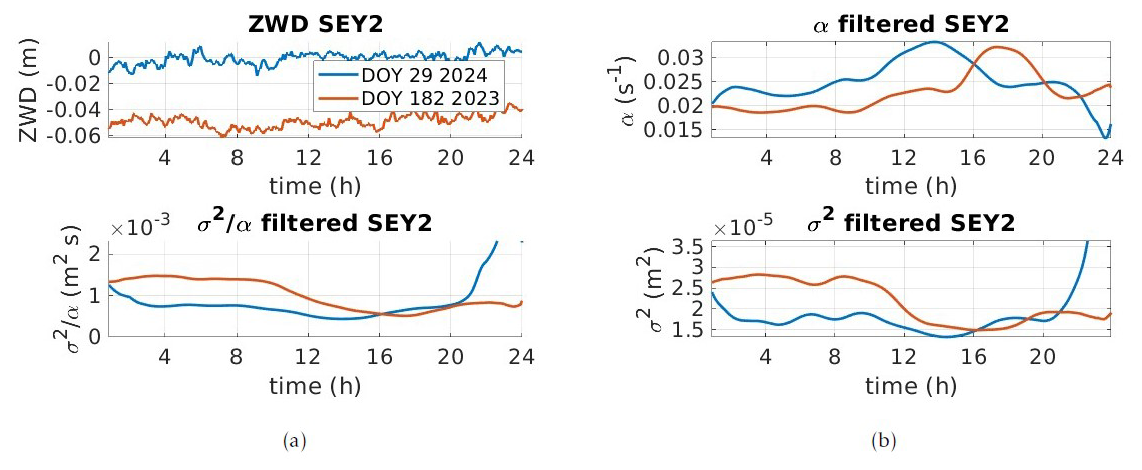
Figure 8 Station SEY2 (tropical climate) (a) top – ZWD (m) for DOY 29 (2024) and DOY 182 (2023); bottom – the ${\mathit{\sigma }}^{\mathrm{2}}/\mathit{\alpha }$ ratio. For panel (b), the top is the cutoff frequency α and the bottom the variance σ². ZWD is used here to mean ZWD corrections.

Indeed, for the 2 d, DOY 29 (2024) and DOY 182 (2023) (summer and winter), no strong variations in the ZWD can be identified in Fig. 8a  top. However, for the selected days, we observe a decrease in σ² after 10:00 UTC, linked to an increase in α at the same time. This effect is stronger during winter (Southern Hemisphere, red line) than in summer. It is most probably due to local atmospheric processes, maybe an increase in the convection at the sea level during the day. We note strong periodic variations (distance minima/maxima of 4 h or less for the other stations except UNB3). The minimum of σ² (maximum of α) is delayed in winter compared to summer (14:00 versus 18:00 UTC), an effect that could be physically explainable by, e.g. the time at which the maximum temperature is reached (as the buoyancy would increase). Due to the location of the station, however, general conclusions should be made carefully.

The ${\mathit{\sigma }}^{\mathrm{2}}/\mathit{\alpha }$ ratio is nearly constant before and after 10:00 UTC and slightly higher for the winter day under consideration, but it is difficult to interpret compared to the other stations. We found close results for 2 d in autumn and spring presented in Appendix B. The periodic variations in α for autumn (Southern Hemisphere, DOY 99 (2024)) were strong, with a period varying from approximately 16:00 UTC (afternoon) to 06:00 UTC (morning). For spring (DOY 274 (2023)), the periodic variations were damped in the late afternoon. This could be linked with specific air mass movement creating buoyancy, thus affecting the end of the inertial range (low-frequency region).

4 Discussion and outlook

Enhancing the understanding of spatiotemporal characteristics of turbulent WV fluctuations will significantly improve models for nowcasting extreme weather events. It will also shed light on turbulent processes in the energy input region, which remain only partially understood. Utilizing cost-effective, all-weather instruments like GNSS receivers, which offer the necessary accuracy, data rate, and spatial coverage worldwide, is a promising solution to reach that goal. This requires the development of a reliable, statistically based method for extracting relevant turbulence parameters from the estimated ZWD.

We have developed a new methodology to extract the turbulent fluctuations by filtering the ZWD from mesoscale effects. An S-G filter was tuned adequately to retrieve the part of the ZWD spectrum that has von Kármán spectrum content. We used a maximum likelihood approach to estimate the turbulent parameters: the cutoff frequency α corresponding to the end of the inertial range using the Taylor frozen hypothesis and the strength of turbulence σ² corresponding to the variance of the filtered (turbulent) process. To investigate the extent to which those parameters may vary depending on the climate zone (or turbulence above the stations), the time of day, or the year (daily or seasonal pattern), we have randomly selected 2 d and five GNSS stations from the IGS network.

We were able to show that the variations in turbulence strength were related to the cutoff frequency in most cases, except at the RIO2 station (Tierra del Fuego) for a day with strong gravity waves. This promising result highlights the high potential of the analysis of the turbulent parameters to deepen our understanding of turbulent processes in the ABL related to WV fluctuations. Differences in winter/summer and day/night were visible for the oceanic and continental climates but not for the tropical climate. We identified some dependencies between expected turbulence characteristics (buoyancy or wind shear) and the increase/decrease in σ² with respect to α. We identified a periodical pattern with a distance of 4 h or less between maxima and minima, which could be related to air masses and surface heating. This effect was slightly stronger during summer.

We point out that a joint interpretation (climate, location of the station) is mandatory for enhancing the global understanding of the time variations in turbulent parameters. The particular shapes found in our example make us confident that machine learning strategies could be used to identify the main dependencies and perform predictions. Our study is the first milestone in that direction, using easily available worldwide GNSS observations. Validation strategies could include instruments such as eddy covariance (Sun et al., 2018) or large eddy simulations (Maronga et al., 2020). We found promising dependencies using a gradient boosting algorithm, such as was used in Pierzyna et al. (2024), with the vertical wind velocity and the total kinetic energy retrieved from lidar measurements at a 1500 m height. Confirmation and a proof of concept are still required.

Appendix A: RIO2: gravity waves

In this Appendix, we show the potential impact of gravity on the cutoff frequency α. To reach that goal, we have selected 1 d from https://worldview.earthdata.nasa.gov/ (last access: 5 January 2025) during which gravity waves above RIO2 (located as shown in http://geodesy.unr.edu/NGLStationPages/stations/RIO2.sta, last access: 5 January 2025) could be visually identified from the corrected reflectance (DOY 135 (2024)). The Visible Infrared Imaging Radiometer Suite (VIIRS) corrected reflectance imagery is available in near real time from the Suomi NPP satellite, operated by NASA and the NOAA. This imagery has a daily sensor resolution of 750 and 375 m. For comparison, we also computed DOYs 134 and 136 (the red and yellow lines, respectively in Fig. A1). The ZWD for the 3 d under consideration does not exhibit strong variations, i.e. a light continuous increase for DOYs 134 and 136 only. The values for σ² highlight an increase in turbulence in the evening from 16:00 to 20:00 UTC and a periodic pattern, as shown in Fig. 7. On DOY 136, σ² is nearly constant, with a light wavy shape. This latter is also visible in α, with a nice correspondence between the minima and maxima of the two quantities. Similar behaviour is visible for DOY 135 (yellow line). However, on DOY 134 (blue line), it is evident that the strong maximum of α around 13:00 UTC is not linked to a minimum of σ² as usual. We are inclined to think that this behaviour could be due to the gravity waves; these would affect the low-frequency region of the spectrum associated with large scales without impacting the strength of the turbulence. This remains to be confirmed in a subsequent contribution but already highlights the high potential of ZWD to study specific atmospheric effects in the ABL related to turbulence.

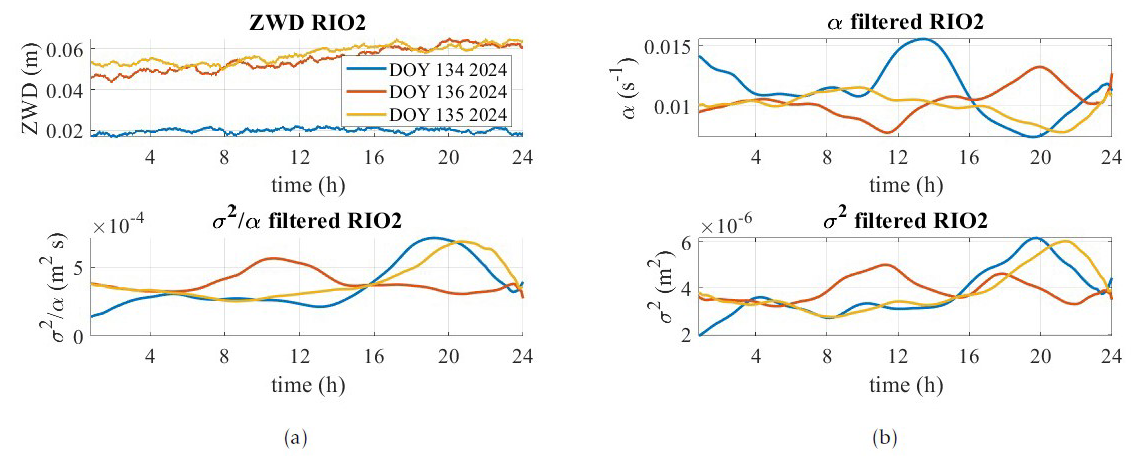
Figure A1 Station RIO2 (gravity waves) (a) top – ZWD (m) for DOY 134 (2024), DOY 135 (2024), and DOY 136 (2024); bottom – the ${\mathit{\sigma }}^{\mathrm{2}}/\mathit{\alpha }$ ratio. For panel (b), the top is the cutoff frequency α and the bottom the variance σ².

Appendix B: SEY2: autumn and spring

For the sake of completeness and because the spring and autumn seasons may be slightly different than summer and winter for the tropical climate, we have added 2 d, DOY 99 (2024) and DOY 274 (2023), presented in Fig. B1. The description and analysis are provided in the main body.

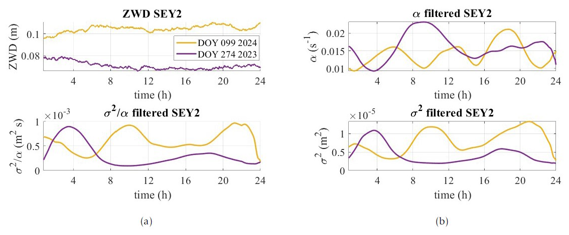
Figure B1 Station SEY2 (tropical climate) (a) top – ZWD (m) for DOY 099 (2024), and DOY 273 (2023); bottom – the ${\mathit{\sigma }}^{\mathrm{2}}/\mathit{\alpha }$ ratio. For panel (b), the top is the cutoff frequency α and the bottom the variance σ².