Modelled surface climate response to effusive Icelandic volcanic eruptions: sensitivity to season and size

Effusive, long-lasting volcanic eruptions impact climate through the emission of gases and the subsequent production of aerosols. Previous studies, both modelling and observational, have made efforts to quantify these impacts and untangle them from natural variability. However, due to the scarcity of large and well-observed effusive volcanic eruptions, our understanding remains patchy. Here, we use an Earth system model to systematically investigate the climate response to high-latitude, effusive volcanic eruptions, similar to the 2014–2015 Holuhraun eruption in Iceland, as a function of eruption season and size. The results show that the climate response is regional and strongly modulated by different seasons, exhibiting midlatitude cooling during summer and Arctic warming during winter. Furthermore, as eruptions increase in size in terms of sulfur dioxide emissions, the climate response becomes increasingly insensitive to variations in emission strength, levelling off for eruptions between 20 and 30 times the size of the 2014–2015 Holuhraun eruption. Volcanic eruptions are generally considered to lead to surface cooling, but our results indicate that this is an oversimplification, especially in the Arctic, where warming is found to be the dominant response during autumn and winter.

1 Introduction

Volcanic eruptions vary greatly in their behaviour. Some are dominated by explosive activity, where magma explodes and is erupted as tephra. In other cases, explosive activity is mostly absent, and the magma is mainly erupted as lava. Eruptions falling into the latter group are referred to as effusive eruptions. Their emissions stay close to the ground, mostly in the lower and middle troposphere. They release various gaseous species, with water vapour, carbon dioxide, and sulfur dioxide being the most prominent (e.g. Textor et al., 2004). Of these gases, sulfur dioxide (SO₂) is the most relevant to short-term climate impacts as it is a precursor to sulfate (SO₄) aerosols (Robock, 2000). These aerosols mainly impact climate through interactions with radiation, doing so either directly (Graf et al., 1998) or indirectly by acting as cloud condensation nuclei (CCN) via various aerosol–cloud interactions (Gassó, 2008).

Previous studies have observed shortwave radiative forcing due to aerosol–cloud interactions (i.e. more numerous cloud droplets and higher cloud albedo with increased CCN concentrations) (Twomey, 1977) as a result of effusive volcanic emissions. Examples include the 2008 and 2018 Kīlauea eruptions in Hawaii (Eguchi et al., 2011; Breen et al., 2021), the 2012 Mount Curry eruption in the South Sandwich Islands (Schmidt et al., 2012), and the 2014–2015 Holuhraun eruption in Iceland (Gettelman et al., 2015; McCoy and Hartmann, 2015; Malavelle et al., 2017). Adjustments to aerosol–cloud interactions (Albrecht, 1989) have also been identified, with evidence of a significant increase in cloud cover during the first months of the 2014–2015 Holuhraun eruption (Chen et al., 2022), as well as during the 2008 and 2018 Kīlauea eruptions (Chen et al., 2024). In our previous study (Zoëga et al., 2023), we demonstrated – using observational data, reanalysis, and model simulations – that the 2014–2015 Holuhraun eruption led to surface warming in the Arctic during the early winter of 2014–2015. This warming was driven by an increased liquid water path, along with increased cloud cover and the subsequent trapping of longwave radiation under limited sunlight.

Iceland is volcanically active, having experienced an average of 20 to 25 eruptions per century over the past ∼ 1100 years. These eruptions have varied greatly in size and characteristics, with roughly one out of every five being either effusive or mixed effusive–explosive (Thordarson and Larsen, 2007). Examples include the 1783–1784 Laki eruption, which is estimated to have emitted a total of 122 Tg SO₂ over a period of 8 months (Thordarson and Self, 2003), and the 939–940 Eldgjá eruption, which emitted around 220 Tg SO₂ over a period of at least 1.5 years (Thordarson et al., 2001; Oppenheimer et al., 2018; Hutchison et al., 2024). The great Þjórsárhraun eruption (which occurred around 8000 years before present) is thought to have been the largest effusive eruption on Earth during the Holocene, with a lava production of at least 21 km³ (Hjartarson, 1988; Siebert et al., 2010). For reference, the lava production of the 1783–1784 Laki and 939–940 Eldgjá eruptions amounted to about 15 and 20 km³, respectively (Thordarson and Self, 1993; Thordarson et al., 2001; Sigurðardóttir et al., 2015). Closer in time is the aforementioned 2014–2015 Holuhraun eruption, which emitted up to 9.6 Tg SO₂ over a period of 6 months (Pfeffer et al., 2018) and produced about 1.2 km³ of lava (Bonny et al., 2018). Icelandic volcanoes, therefore, have a history of very large, long-lasting effusive eruptions.

It is only during the past few decades that we have been able to accurately monitor high-latitude volcanic eruptions and their climate impacts – namely, since the beginning of the satellite era (Robock, 2000; Carn et al., 2016). The focus has mostly been on explosive eruptions (Haywood et al., 2010; Kravitz et al., 2010; Andersson et al., 2015), and their climate impacts have been shown to highly depend on factors such as eruption latitude, season, and size; emission altitude; and the atmospheric background state (e.g. Schneider et al., 2009; Kravitz and Robock, 2011; Toohey et al., 2019; Zambri et al., 2019; Marshall et al., 2020; Fuglestvedt et al., 2024; Zhuo et al., 2024). Despite considerable research efforts in recent years, the climate impacts of high-latitude effusive eruptions remain less understood, particularly in relation to environmental and eruptive parameters. Here, we address this issue using an Earth system model and systematically investigate the climate response to idealized high-latitude, long-lasting effusive volcanic eruptions as a function of eruption season and emission strength.

2 Methods

2.1 Model

We simulate the climate response to a range of effusive volcanic eruptions using version 2.1.3 of the Community Earth System Model in combination with version 6 of the Community Atmosphere Model, referred to as CESM2(CAM6) (Danabasoglu et al., 2020). This model has 32 vertical levels, which extend to an altitude of 2.26 hPa (ca. 40 km). For the horizontal resolution, we use 0.9° latitude by 1.25° longitude. All of our simulations are coupled with active atmosphere, ocean, sea ice, and land components.

CESM2(CAM6) includes a simplified sulfur chemistry scheme, as described by Barth et al. (2000), which simulates both the gas-phase and aqueous oxidation of SO₂ into SO₄. The atmospheric oxidants ozone (O₃) and the hydroxyl radical (OH), along with stratospheric aerosols, are prescribed from CESM2-based historical Coupled Model Intercomparison Project Phase 6 (CMIP6) simulations using the Whole Atmosphere Community Climate Model (WACCM) (Gettelman et al., 2019). The four-mode version of the Modal Aerosol Module (MAM4) (Liu et al., 2016) simulates the formation and development of tropospheric aerosols. The four log-normal aerosol modes of MAM4 are the Aitken, accumulation, coarse, and primary-carbon modes. Together, they include sulfate, sea salt, primary and secondary particulate organic matter, black carbon, and soil dust, which are internally mixed within each mode. The conversion of aerosol from one mode to another is simulated through coagulation and condensation (Liu et al., 2012, 2016). The second version of the Morrison–Gettelman scheme (MG2) (Gettelman and Morrison, 2015) is used for prognostic cloud microphysics.

CESM2(CAM6) includes the unified turbulence scheme Cloud Layers Unified By Binormals (CLUBB) (Golaz et al., 2002). In CLUBB, cloud entrainment processes that could lead to a deceased LWP are controlled by prognostic vertical turbulent fluxes and a tunable air parcel entrainment rate. However, both the LWP and cloud cover are relatively insensitive to variations in the CLUBB parameter representing the entrainment rate (Guo et al., 2015). In their modelling study (which does not use CLUBB), Karset et al. (2020) found that other factors, such as the sensitivity of the autoconversion rate to cloud droplet number concentration, play an even larger role in controlling the LWP than parameterized entrainment processes.

2.2 Simulations

We carry out a transient control run, corresponding to the model years 2005–2015, using the CMIP6 historical forcing (Eyring et al., 2016). For the year 2015, extensions of the existing historical CMIP6 forcing fields were used when available (van Marle et al., 2017; Hoesly et al., 2018); otherwise, the Shared Socioeconomic Pathway 2-4.5 (SSP2-4.5) forcing (O'Neill et al., 2016) was applied.

From the control run, we branch off a number of simulations where volcanic emissions were added. These branches are 6 months long, and we refer to them as eruption simulations. For each scenario considered in this study (see the following), this leads to 10 eruption simulations, each of which has its own unique initial conditions.

The volcanic eruptions in our simulations are represented by prescribed SO₂ emissions. We construct a standard eruption scenario using petrological estimates of emissions from the 2014–2015 Holuhraun eruption as a reference (Thordarson and Hartley, 2015; Zoëga et al., 2023) (see Fig. 1). Emissions are highest during the first month and gradually decay afterwards. Daily emissions are constant within each month (approximated by 30 d). We then modify this standard scenario to represent eruptions of different sizes. All our eruptions are located at the site of the 2014–2015 Holuhraun eruption (64.9° N, 16.8° W) and last for 180 d, and emissions are well mixed between 1 and 3 km above sea level.

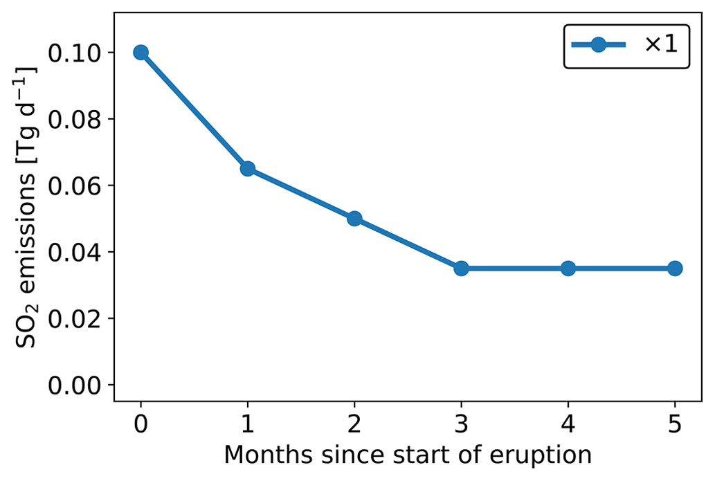
Figure 1 Volcanic SO₂ emission rates for the standard eruption scenario (× 1) used in this study. Daily emissions are constant within each month, well mixed between 1 and 3 km above sea level, and located at the site of the 2014–2015 Holuhraun eruption (64.9° N, 16.8° W).

We are interested in the climate impacts of eruptions of different sizes and therefore vary the strength of the volcanic emissions by multiplying the standard emission scenario shown in Fig. 1 by a range of scaling factors. In addition to the × 1 scaling factor, corresponding to a Holuhraun-sized eruption, we perform simulations using scaling factors of × 5 and × 25, covering the plausible range of effusive Icelandic eruptions, as well as × 50, extending into the size range of the largest known flood basalts on Earth (Kasbohm and Schoene, 2018). We are also interested in how different eruption seasons modulate the climate response and thus perform eruption simulations branched off from the control run on the first days of March, June, September, and December for each model year between 2005 and 2014. This results in 10 eruption simulations for each combination of starting date and magnitude scaling. Throughout this study, we refer to each combination by its scaling factor and start month. For example, a × 5 eruption starting in June is referred to as x5jun.

2.3 Observations and reanalysis

To supplement the model simulations, we examine data from version 5 of the European Centre for Medium-Range Weather Forecasts (ECMWF) Reanalysis (ERA5) (Hersbach et al., 2020, 2024) and time series of observed surface air temperatures. The observational time series are from Svalbard Airport (Svalbard lufthavn) and Jan Mayen (NCCS, 2023), Danmarkshavn and Ittoqqortoormiit (DMI, 2023), and Grímsey (Icelandic Met Office, 2024).

2.4 Anomalies and significance

For a variable (y) from our simulations, we calculate absolute anomalies as follows:

$$\begin{array}{}\text{(1)}& {\left(\mathrm{\Delta }y\right)}_{\mathrm{abs}}=y_{\mathrm{erupt}}-y_{\mathrm{contr}}.\end{array}$$

And we calculate relative anomalies as follows:

$$\begin{array}{}\text{(2)}& {\left(\mathrm{\Delta }y\right)}_{\mathrm{rel}}={\displaystyle \frac{y_{\mathrm{erupt}}-y_{\mathrm{contr}}}{y_{\mathrm{contr}}}}.\end{array}$$

This results in an ensemble of 10 sets of anomalies for each combination of scaling factor and start month. The two simulations being compared (i.e. the control and eruption) match with respect to all background conditions (initial meteorology, background emissions, greenhouse gas concentrations, etc.) and only differ in a single aspect: the volcanic SO₂ emissions. This approach is referred to as a matched-pairs analysis (e.g. Barlow, 1993).

For a measure of confidence, we calculate 95 % confidence intervals (CIs) based on a two-tailed t test as follows:

$$\begin{array}{}\text{(3)}& \mathrm{CI}=\mathit{\mu }\pm t^{\ast }\cdot \widehat{\mathit{\sigma }},\end{array}$$

where μ is the 10-member ensemble mean, t^∗ is an appropriate value from the t statistics, and $\widehat{\mathit{\sigma }}=\mathit{\sigma }/\sqrt{n}$ refers to the standard error in the ensemble. Here, σ is the standard deviation of the ensemble, and n=10 is the number of ensemble members.

For the observational time series and ERA5 reanalysis, anomalies are calculated with respect to a linear fit for the 30-year period from 1984 to 2013. The constructed 95 % prediction interval is calculated as ±1.96 σ from the mean of the detrended 1984–2013 time series, with σ being the standard deviation of the time series.

2.5 Logarithmic fit and growth rate

To investigate the climate response as a function of eruption size, we fit a logarithmic curve to the set of anomalies (Δy) as follows:

$$\begin{array}{}\text{(4)}& \mathrm{\Delta }{y}_{\mathrm{fit}}=a\ln (bx+\mathrm{1}),\end{array}$$

where x represents the magnitude scaling factors and a and b represent the fitting coefficients. We calculate a and b using the method of least squares. A value of 1 is added to bx to satisfy $\mathrm{\Delta }{y}_{\mathrm{fit}}(x=\mathrm{0})=\mathrm{0}$, meaning there are no anomalies in the case of no eruption. We further calculate a growth rate (GR), which represents the relative change in Δy_fit per magnitude scaling factor, such that

$$\begin{array}{}\text{(5)}& \mathrm{GR}={\displaystyle \frac{\mathrm{1}}{y}}\cdot {\displaystyle \frac{\mathrm{d}}{\mathrm{d}x}}\left(\mathrm{\Delta }{y}_{\mathrm{fit}}\right)={\displaystyle \frac{\mathrm{1}}{y}}\cdot {\displaystyle \frac{a}{x+\mathrm{1}/b}}.\end{array}$$

3 Results

Due to the high number of simulations performed in this study, we focus on the x5jun and x5dec eruptive scenarios for illustrative purposes (unless otherwise stated). We choose eruptions starting in June and December as we expect the climate response from summer and winter eruptions to generally represent the extremes at both ends of the response spectrum. We choose the × 5 scaling scenario as such eruptions are both very large and realistic, being approximately halfway between the 2014–2015 Holuhraun eruption and the 1783–1784 Laki eruption in terms of mean SO₂ emission rate.

3.1 SO₄ aerosols and CCN

The conversion of SO₂ gas to SO₄ aerosols is controlled by the oxidation capacity of the atmosphere, which, in turn, depends largely on sunlight availability. SO₄ aerosol production from precursor gases is therefore highly seasonal. This can clearly be seen in our simulations, where the volcanic aerosol load is much higher during the first 3 months of eruptions starting in June (June to August (summer); see Fig. 2a) compared to during the first 3 months of eruptions starting in December (December to February (winter); see Fig. 2d). This seasonal difference is largest in the Arctic, as defined by the Arctic Circle, where the aerosol load is 5.8±1.5 times higher during summer than during winter in our × 5 simulations.

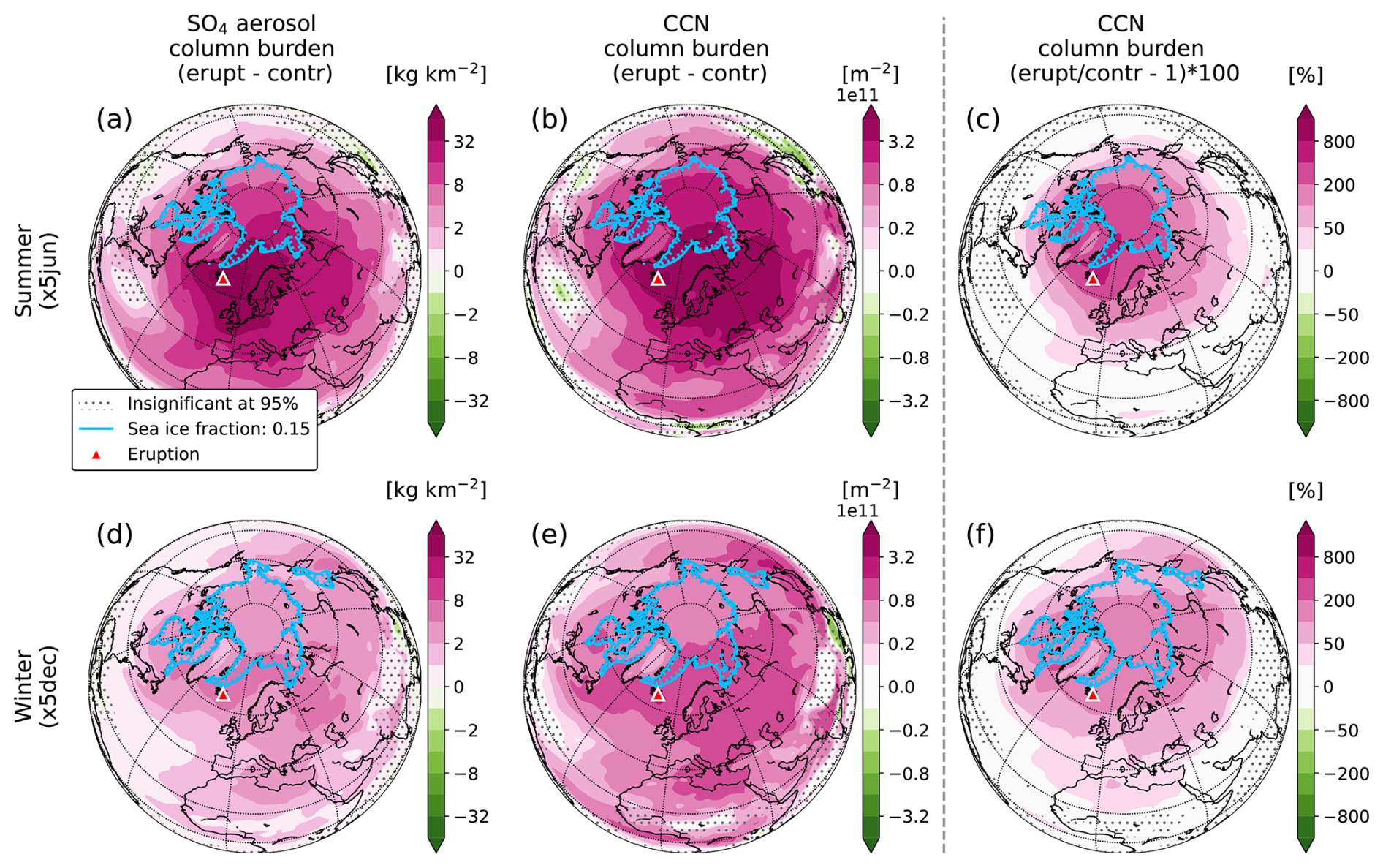
Figure 2 Ensemble mean absolute anomalies from the CESM2(CAM6) simulations for the first 3 months of an eruption with respect to the SO₄ aerosol column burden for the (a) x5jun and (d) x5dec scenarios and with respect to the CCN (0.1 % supersaturation) column burden for the (b) x5jun and (e) x5dec scenarios. To the right of the vertical dashed line, relative CCN column burden anomalies are displayed for (c) summer and (f) winter. The dotted regions indicate insignificance at the 95 % confidence level, calculated with a two-tailed t test, and the blue contours represent the mean sea ice edge for the first 3 months of the eruption, based on the eruption runs (with a sea ice cover of 15 % defining the sea ice edge). Summer corresponds to the June–August mean, and winter corresponds to the December–February mean. In the figure titles, erupt refers to eruption simulations and contr to the control run.

SO₄ aerosols are very hygroscopic and therefore effective as CCN (e.g. Hobbs, 2000). In our simulations, the modelled SO₄ aerosol perturbations dominate the distribution of CCN (Fig. 2b and e), as evident when comparing the spatial patterns of the aerosol and CCN anomalies. In both cases, the dominant transport direction is toward the northeast – namely, over the Greenland and Norwegian seas, across northern Eurasia, and into the Arctic. We also observe smaller, but still significant, aerosol anomalies covering much larger areas, stretching from the central North Atlantic across North Africa, the Mediterranean Sea, and central Asia and extending all the way into the North Pacific and the Bering Sea. This applies to both summer and winter. The main difference between the seasons is the magnitude of the anomalies. The relative anomalies reveal a different pattern, especially in the case of the CCN (Fig. 2c and f). The greatest relative CCN anomalies occur in the Arctic, exhibiting up to a 5-fold increase in summer and more than doubling in winter. This is due to the low background CCN levels in the Arctic (Fig. A1a and d) (Choudhury and Tesche, 2023), which result from the region's relatively weak local CCN sources and its long distance from stronger sources at lower latitudes (e.g. Bigg and Leck, 2001).

3.2 Cloud droplets

Since SO₄ aerosols are effective as CCN, they can considerably alter cloud properties. Generally speaking, we expect a positive CCN perturbation to increase the number of cloud droplets and decrease their size (Twomey, 1977).

In the CCN-poor Arctic, clouds are particularly sensitive to CCN perturbations. During the relatively warm and moist summer, this results in few but large cloud droplets (Fig. A1b and c). In our eruption simulations, we observe an increase in the number of cloud droplets (Fig. 3a), closely resembling the pattern of relative CCN increase. As expected, the cloud droplets also shrink considerably (Fig. 3b), especially over the Arctic sea ice, where they are the largest in the control run. Contrary to the summer response, which is mainly in the Arctic, the largest cloud droplet anomalies during winter are found over the Labrador Sea and the Sea of Okhotsk, followed by the open-ocean areas off the Arctic sea ice edge in the Atlantic sector. Cold-air outbreaks from Canada, Siberia, and Arctic sea ice transport cold, CCN-poor air over the open ocean, leading to the formation of clouds with few but large droplets (Fig. A1e and f). These clouds are particularly sensitive to CCN perturbations and respond strongly by increasing the number of droplets and decreasing their size (Fig. 3c and d).

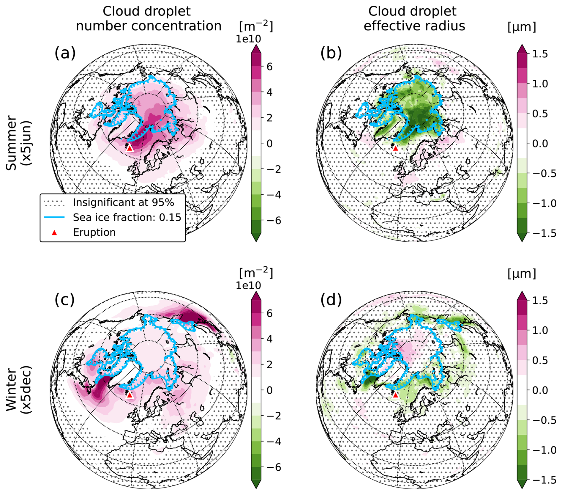
Figure 3 As in Fig. 2 but for vertically integrated cloud droplet number concentration (a, c) and the vertically averaged cloud droplet effective radius (b, d).

3.3 Cloud lifetime

By increasing the number of cloud droplets and decreasing their size, CCN perturbations have the potential to affect the liquid water content of clouds as well as their horizontal and vertical extent (Albrecht, 1989). We simulate a significant increase in the cloud liquid water path (LWP), both in summer and winter (Fig. 4a and c, respectively), which correlates well with the increased cloud droplet number concentration.

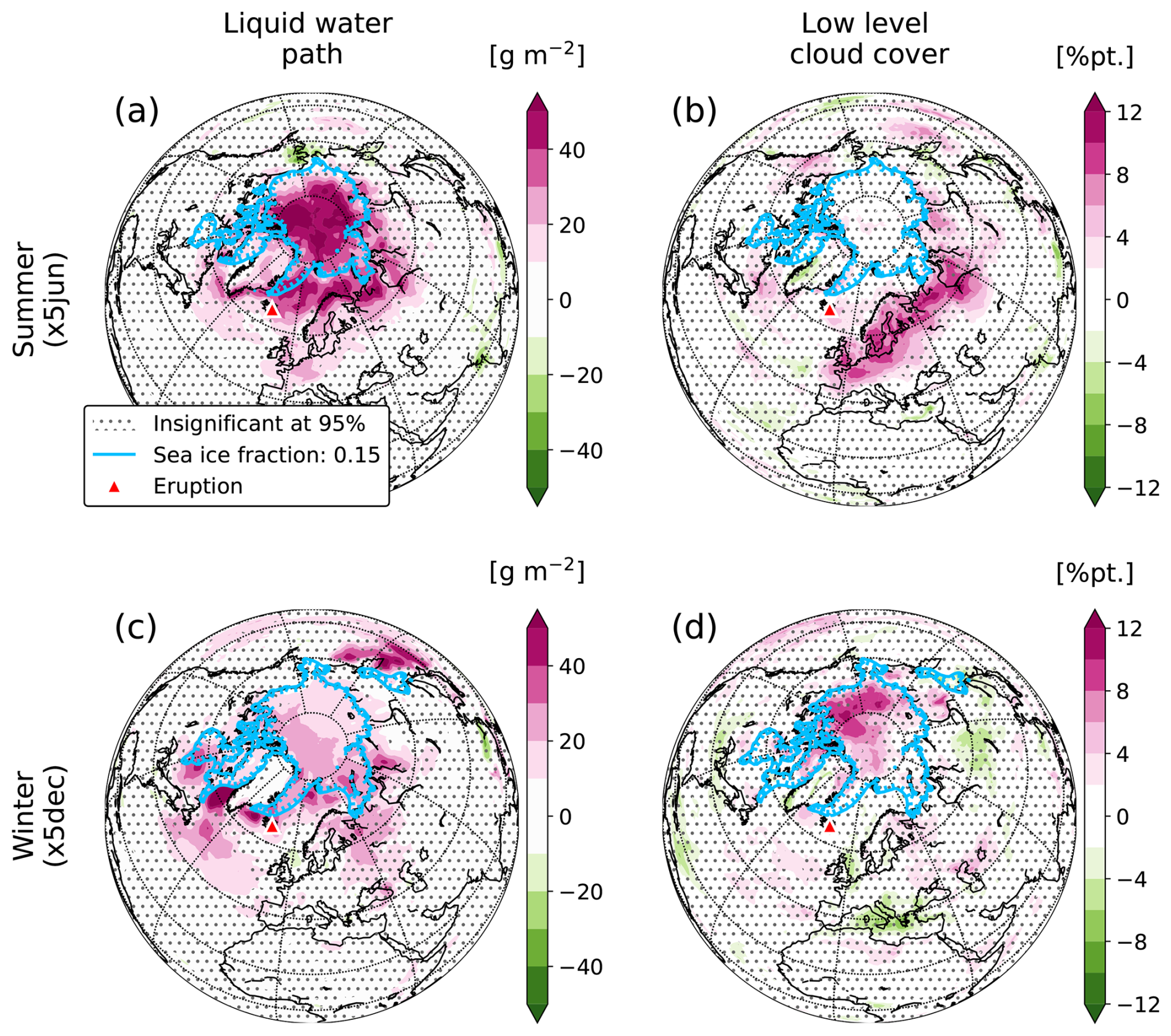
Figure 4 As in Fig. 2 but for the vertically integrated liquid water path (a, c) and low-level cloud cover (b, d).

In summer, this LWP increase is mainly confined to the Arctic. It can be explained by delayed precipitation due to smaller cloud droplets and slower collision–coalescence processes over the sea ice in the central Arctic and by suppressed precipitation over the ice-free Nordic seas (Fig. A3b). Cloud cover over the Arctic remains unaffected (Fig. 4b) since the Arctic is already mostly overcast in summer (Fig. A2b) (Curry et al., 1996). However, we do simulate increased low-level cloud cover over northern Europe, where background cloud cover is lower than in the central Arctic.

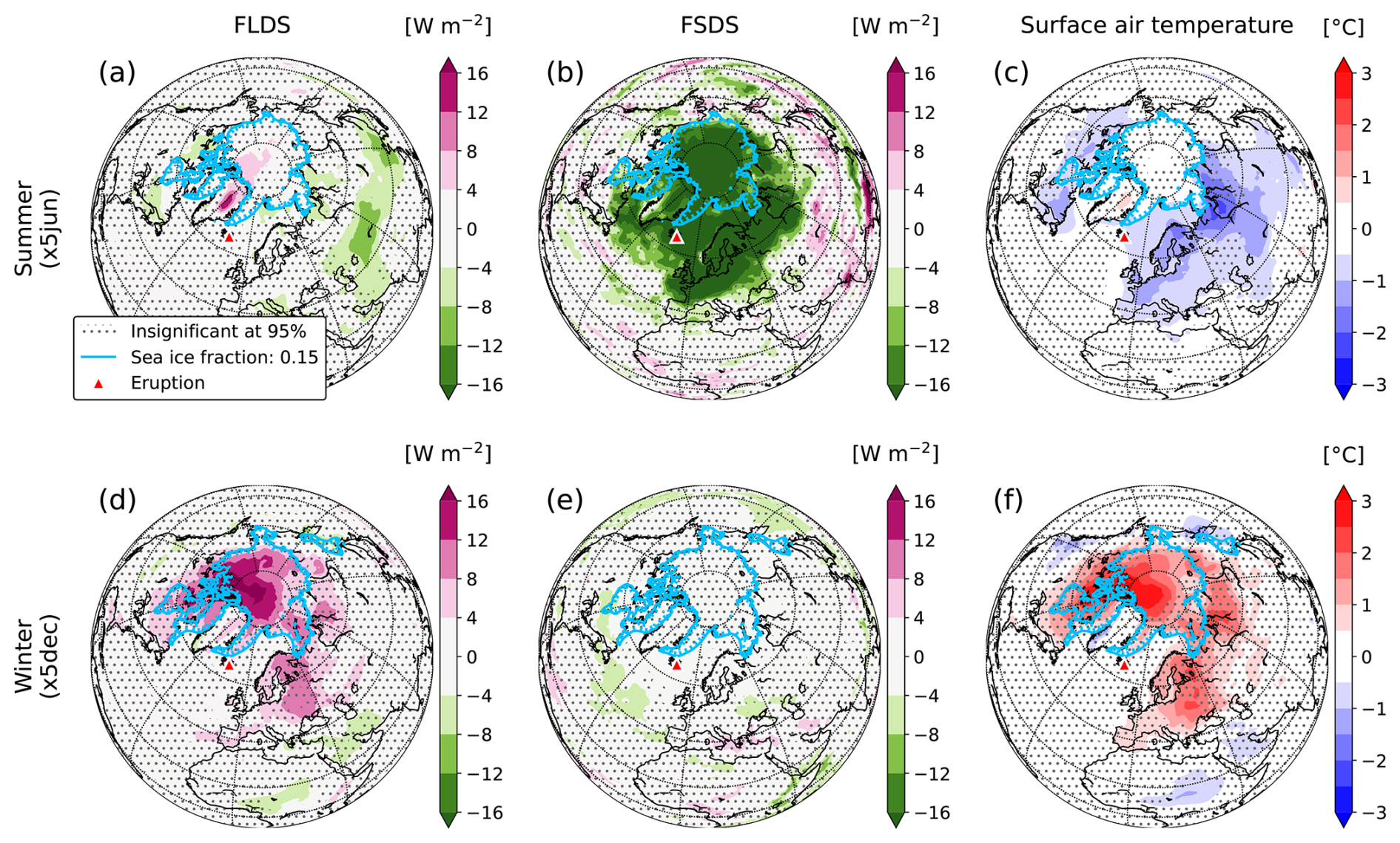
Figure 5 As in Fig. 2 but for downward longwave radiative flux at the surface (FLDS) (a, d), downward shortwave radiative flux at the surface (FSDS) (b, e), and surface air temperature (c, f).

Delayed or suppressed precipitation also explains the increased LWP in winter over the Labrador Sea and the Sea of Okhotsk (Fig. 4c), where we see a small but significant precipitation reduction (Fig. A3d), accompanied by a cooling signal (Fig. 5f). This is, however, not the case in the central Arctic, where the model shows a significant increase in the LWP, despite the near absence of precipitating clouds (Fig. A3c). Accordingly, we suggest the following.

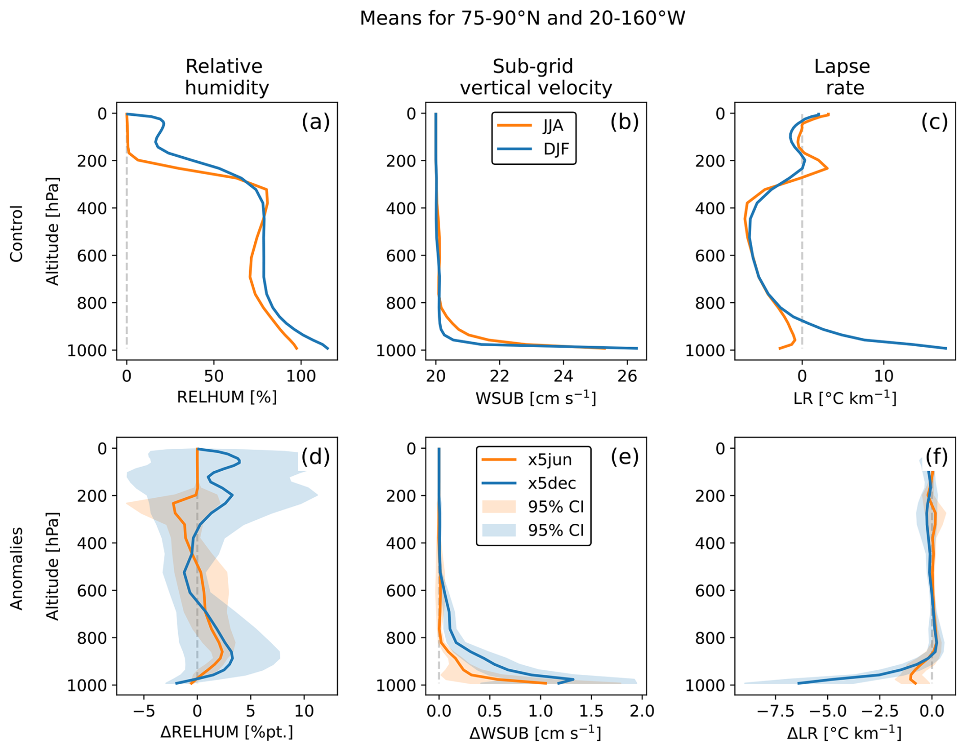
Increased droplet number concentration at the edge of the Arctic Basin leads to a local increase in the LWP. This results in increased trapping of longwave radiation and subsequent surface warming (see Sect. 3.4 and 3.5). This warming induces a deeper subpolar low in the North Atlantic, accompanied by stronger southerly winds that advect warm air into the Arctic (Fig. A11d). With a warmer Arctic, the liquid water content of ice-containing clouds increases, which results in larger liquid cloud droplets in the central Arctic in our simulations (Fig. 3d). It is well established that when the ratio of liquid to ice water content in clouds increases, cloud precipitation is generally less efficient (the Wegener–Bergeron–Findeisen process) and cloud lifetimes increase (e.g. Tsushima et al., 2006; Storelvmo et al., 2011; Tan and Storelvmo, 2019). This explains the increased cloud cover and LWP in the wintertime Arctic Basin. This process is represented in CESM2(CAM6). The resulting surface warming weakens the strong temperature inversion in the central Arctic (Fig. A5f), leading to increased updraft (Fig. A5e) and yet more cloud formation.

3.4 Surface radiation

When the LWP ≳ 30 g m⁻², clouds become opaque in the longwave (LW) part of the radiative spectrum (Slingo et al., 1982; Shupe and Intrieri, 2004), meaning that once this threshold is passed, an increase in the liquid water content of clouds will not affect their ability to absorb and emit LW radiation. This is the case in our simulations in the Arctic during summer, where the background LWP is about 140 g m⁻² (Fig. A2a). As a result, the LW trapping abilities of the low-level Arctic clouds, as represented by the downward LW flux at the surface (FLDS; Fig. 5a), only marginally increase in the summer months, despite the considerable LWP increase. The winter is a different story. Here, the mean LWP over the Arctic sea ice is about 40 g m⁻², dropping below 25 g m⁻² north of Greenland and Canada. The relatively modest LWP increase over the Arctic sea ice, along with the increased low-level cloud cover, therefore leads to a strong increase in the LW trapping of the clouds in that area. In our x5dec simulations, the model shows an Arctic mean December–February FLDS increase of almost +8 W m⁻², reaching more than +16 W m⁻² in the central Arctic (Fig. 5d).

For the shortwave (SW) part of the radiative spectrum, radiative extinction increases with an increasing LWP for a much wider LWP range (e.g. Han et al., 1998; Glenn et al., 2020). While absorption and re-emission dominate in the LW part of the spectrum, scattering plays a major role in SW radiation, with smaller particles scattering more efficiently than larger ones (e.g. Fouquart et al., 1990). As a result, the model shows a strong decrease in downward SW flux at the surface (FSDS) across the entire Arctic and northern Europe during summer (Fig. 5b), closely coinciding with the increased LWP and decreased cloud droplet size. In our x5jun simulations, the model shows an Arctic mean June–August FSDS decrease of almost −17 W m⁻². During winter, sunlight is limited at high latitudes and largely absent in the Arctic; hence, the model hardly shows any SW anomalies (Fig. 5e).

Direct interactions between SO₄ aerosols and radiation are highly wavelength-dependent. While SO₄ aerosols have a minimal impact on LW radiative transfer, they effectively attenuate SW radiation, doing so mainly through scattering (Kiehl and Briegleb, 1993; Clapp et al., 1997). In the Arctic, we would therefore expect direct aerosol effects to be most effective during summer and negligible during winter. This is the case in our simulations. The model shows an increase in the summertime aerosol optical depth at 550 nm of around 0.5 over the Greenland and Norwegian seas (Fig. A6a), with anomaly patterns closely following the modelled volcanic SO₄ aerosol load. As a result, the clear-sky component of the downward SW surface flux (FSDSC; Fig. A6b) plays a considerable role in SW radiative transfer during summer. Surface radiative fluxes therefore depend on both direct and indirect aerosol effects during summer, whereas the indirect effects – namely, aerosol–cloud–radiation interactions – dominate during winter.

3.5 Surface air temperature

When it comes to surface air temperatures, the model shows pronounced warming in the Arctic during winter (Fig. 5f). This warming is widely significant and reaches more than +3 °C in remote areas north of Canada and Greenland. The reason for this warming is the trapping of LW radiation under limited sunlight due to increased low-level cloud cover and an increased LWP, as discussed in the previous sections.

During summer, there are significant cooling anomalies over northern Eurasia and North America, reaching more than −2 °C over Siberia. The model also shows cooling of more than −1 °C over the Greenland, Norwegian, and Barents seas. Interestingly, there is hardly any significant temperature response over the Arctic sea ice during summer. We interpret this as mainly a result of the relatively high albedo of the sea ice and reduced sea ice melting.

Multiple reflections between low-level clouds and the ground play an important role in SW surface radiative forcing. Where clouds cover bright surfaces, these reflections considerably reduce the effectiveness of the SW cloud shielding. This effect is well known and has been observed in the Arctic (Wendler et al., 1981). In our simulations, it is clearest during spring and early summer, when the model shows a small reduction in downward SW flux over the Arctic sea ice compared to over the open-ocean areas off the sea ice edge (Fig. A7b). The multiple-reflection effect is especially sensitive to variations in ground albedo at high albedo values, with its effectiveness sharply decreasing during late summer as the Arctic sea ice fraction decreases. Over dark surfaces, e.g. the open ocean, these reflections play a minor role. Additionally, increased cloud shielding from direct sunlight decreases sea ice melt, leading to less heat from the atmosphere being absorbed by the sea ice (Fig. A8b).

Additionally, the model shows an increase in the Arctic sea ice fraction following the start of the x5jun eruptions (Fig. A8b). This increase is observed across the Arctic but is most prominent outside of the central Arctic, where the background sea ice fraction is between 50 % and 60 %. Here, the model shows an increase of up to +15 % pt (percentage points). This indicates that the shielding effects of the clouds slow down the sea ice melt during summer, making the Arctic surface more reflective and amplifying the SW reflection effect discussed above. The Arctic sea ice response during winter is not as widespread. However, the model shows a December–February change in sea ice fraction of up to −10 % pt following the start of the x5dec eruption occurring along the sea ice edge in the Greenland, Barents, and Bering seas (Fig. A8d).

3.6 Seasonal cycle

Until now, we have focused on eruptions starting in summer and winter. To get a fuller picture of the seasonal cycle, we add simulations for eruptions starting in March (x5mar) and September (x5sep) and look at monthly means for the region of the Arctic, as defined by the Arctic Circle (Fig. 6).

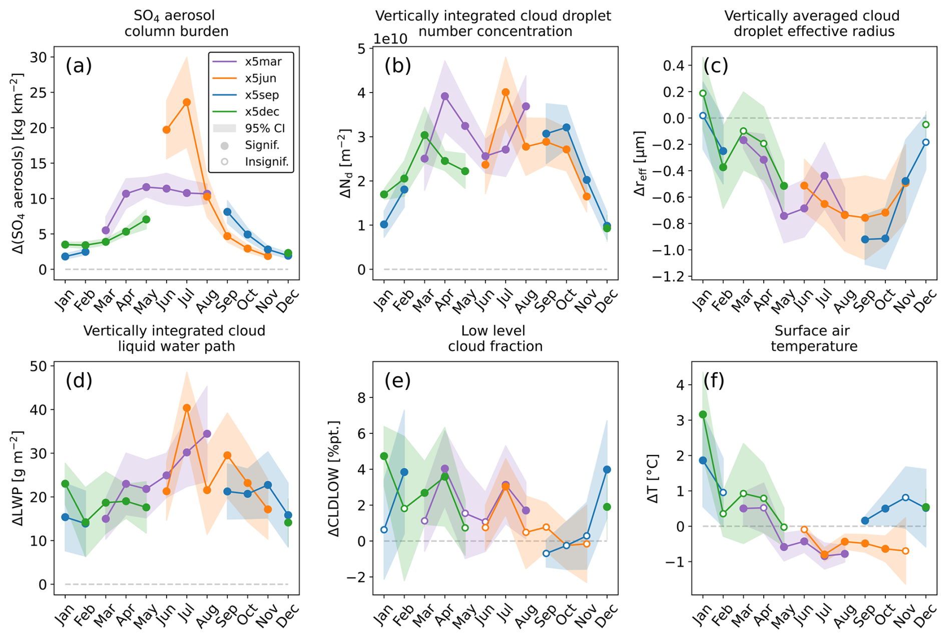
Figure 6 Monthly mean anomalies for the Arctic (as defined by the Arctic Circle) with respect to four different eruption scenarios, starting in March (x5mar), June (x5jun), September (x5sep), and December (x5dec), for the following: (a) the SO₄ aerosol column burden, (b) vertically integrated cloud droplet number concentration, (c) the vertically averaged cloud droplet effective radius, (d) the vertically integrated cloud liquid water path, (e) low-level cloud fraction, and (f) surface air temperature. Shading indicates 95 % confidence intervals based on a two-tailed t test. Filled dots indicate anomalies significantly different from zero, while unfilled dots represent anomalies that differ insignificantly from zero. N_d stands for cloud droplet number concentration, r_eff for cloud droplet effective radius, CLDLOW for low-level cloud cover, and T for temperature.

For the SO₄ aerosol load, cloud droplet number concentration, cloud droplet effective radius, and LWP, the model shows clear seasonal variations, with the largest responses observed in summer and the smallest in winter. The main reason for this is the pronounced seasonality of SO₄ aerosol formation, which depends largely on available sunlight. The low-level cloud cover displays the opposite behaviour, with anomalies being largest in winter and smallest in autumn. This is due to the background conditions as the Arctic is almost completely overcast during the summer months; hence, only a small increase in cloud cover is to be expected.

In some instances, anomalies from different eruption scenarios are significantly different from each other, despite covering the same months. This is clearest for the aerosol anomalies. The reason for this is the gradual decay of emissions in our eruption scenarios, which results in less sulfur being available for aerosol formation as the eruption progresses. This has cascading effects, which eventually lead to the apparent discrepancies in the cloud anomalies.

During mid-winter, there is surface warming in the Arctic of up to +3 °C. The confidence intervals are broad, indicating a large uncertainty in the magnitude of this warming. Despite this, the model shows significant warming in December and January. In mid-summer, there is moderate cooling of up to −1 °C. The summer cooling is more consistent among the different ensemble members compared to the winter warming, resulting in narrower confidence intervals. During autumn (September–November), there is a discrepancy between the temperature responses of the x5jun and x5sep simulations, with cooling observed in the former and warming in the latter. Unlike for the aerosol and cloud parameters discussed earlier, the main reason for this is not the gradual decay of the volcanic emissions but a delayed response. During the first 3 months of the x5jun eruptions, there is a significant drop in sea surface temperature (SST), spanning large areas of the North Atlantic (Fig. A8a). This cooling extends into autumn and affects the surface air temperature accordingly. Conversely, when the eruptions start in September instead of June, there is no high-latitude SST decrease to counteract the LW trapping effects and, consequently, the warming signal. Here, we have an example of how long-lasting effusive eruptions can lead to cumulative effects. This prolonged cooling signal into autumn from eruptions starting in June appears for all scaling factors considered in this study and increases in magnitude with larger eruptions (not shown here).

The focus of this study is on the instantaneous climate response to volcanic eruptions resulting from interactions between aerosols, clouds, and radiation, but we also observe emerging dynamical effects in our simulations. In addition to the SST effect discussed earlier, the model shows atmospheric circulation changes. Most notably, we find a deepening of the Icelandic subpolar low during winter and a weakening during summer (Fig. A11), resulting in a higher North Atlantic Oscillation (NAO) index in winter and lower one in summer (Fig. A9).

3.7 Eruption size

So far, we have discussed eruptions that are about 5 times the size of the 2014–2015 Holuhraun eruption. Now, we include three additional scaling factors: × 1, × 25, and × 50.

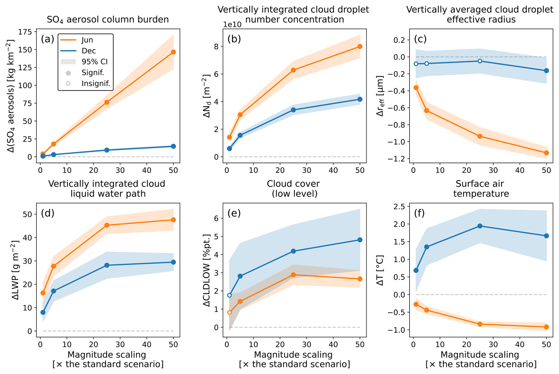
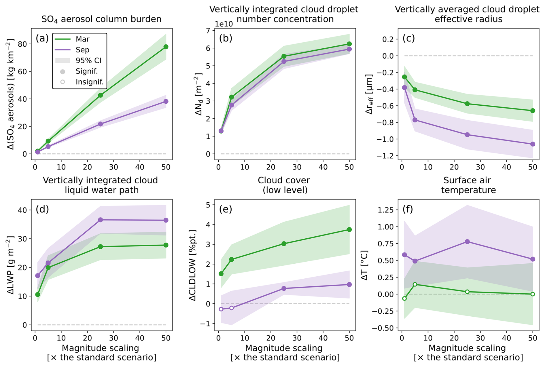
Figure 7 Mean anomalies for the first 3 months of the eruption north of the Arctic Circle, considering four different eruption scaling scenarios (× 1, × 5, × 25, × 50), for the following: (a) the SO₄ aerosol column burden, (b) vertically integrated cloud droplet number concentration, (c) the vertically averaged cloud droplet effective radius, (d) the vertically integrated cloud liquid water path, (e) low-level cloud cover, and (f) surface air temperature. Dots indicate ensemble means, and shading indicates 95 % confidence intervals based on a two-tailed t test. Orange represents eruptions starting in June, and blue represents eruptions starting in December. Filled dots indicate anomalies significantly different from zero, while unfilled dots represent anomalies that differ insignificantly from zero.

Figure 7 shows mean anomalies north of the Arctic Circle for the first 3 months of the eruption as a function of eruption size. The SO₄ aerosol column burden anomalies scale almost linearly with the SO₂ emission strength, both in summer and winter. Since two of the three oxidants responsible for the oxidation of SO₂ in CESM2(CAM6)'s chemistry scheme – i.e. OH and ozone – are prescribed, these oxidants will not become depleted over longer periods of time. Instead, they are replenished at each model time step. This might lead to an overestimation of SO₄ production for the largest eruptions in our simulations. However, similar sulfur chemistry schemes with prescribed oxidants have been used in previous modelling studies investigating aerosols and aerosol–cloud interactions without identifying such issues (e.g. Gettelman et al., 2015; Malavelle et al., 2017; Karset et al., 2018). It is known that stratospheric oxidants become depleted in the plumes of large explosive eruptions, leading to a slower oxidation rate of SO₂ with greater SO₂ emissions and, consequently, non-linear SO₄ aerosol formation in the stratosphere (Pinto et al., 1989; Bekki, 1995; Savarino et al., 2003; Case et al., 2023). This provides motivation for future studies to explore such constraints in tropospheric volcanic plumes rising from large effusive eruptions.

The anomalies of other key variables do not show this linear behaviour but rather level off with eruption size, indicating that clouds become less sensitive to CCN perturbations at higher CCN levels. This saturation effect is well established and expected (e.g. Bellouin et al., 2020; Wang et al., 2024).

Earlier in this study, we discussed how clouds become opaque to LW radiation when the LWP exceeds about 30 g m⁻², thus placing an upper limit on their LW trapping abilities. This is highlighted in Fig. 7f, where the model shows no statistical difference between the winter temperature anomalies in the × 5, × 25, and × 50 scaling scenarios. In the case of the summer cooling, a plateau appears to be reached at much higher emission levels, with the × 25 and × 50 scaling scenarios resulting in significantly stronger cooling than the × 1 and × 5 scenarios. Figure 7f also shows how the ensemble members better agree on the exact magnitude of the summer cooling than that of the winter warming, highlighting the role of large meteorological variability during winter in the Arctic. The spring and autumn anomalies mostly lie between those of summer and winter (Fig. A10). The size of an effusive eruption, therefore, strongly influences the climate response.

4 Discussions

4.1 Extrapolation of the model simulations

Our main goal with this study is to explore the climate response to high-latitude, effusive volcanic eruptions as a function of eruption season and size. Producing a high-frequency dataset – for example, by including more densely spaced magnitude scaling factors – is not viable due to the high computational cost of running an Earth system model. However, by extrapolating the model output, we can gain insight into what happens between our simulated scenarios. One such extrapolation involves fitting the data shown in Fig. 7 to the logarithmic curve described in Eq. (4). Table 1 shows the resulting values of the fitting coefficients a and b.

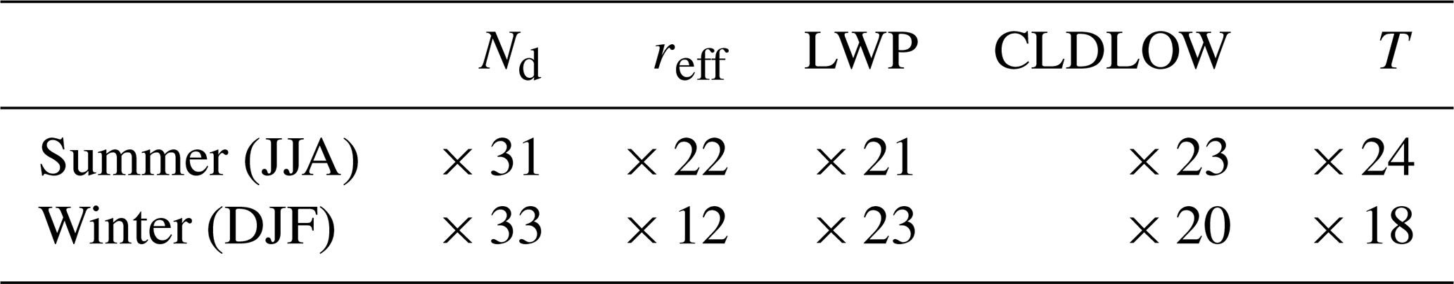
Table 1 The fitting coefficients (a and b) for Eq. (4), corresponding to the variables in Fig. 7 and excluding SO₄ aerosols, which exhibit a nearly linear relationship with volcanic SO₂ emissions. Summer corresponds to the June–August (JJA) mean for eruptions starting in June, while winter corresponds to the December–February (DJF) mean for eruptions starting in December. The unit for the fitting coefficient a is the same as that for the fitted variable, and b is dimensionless.

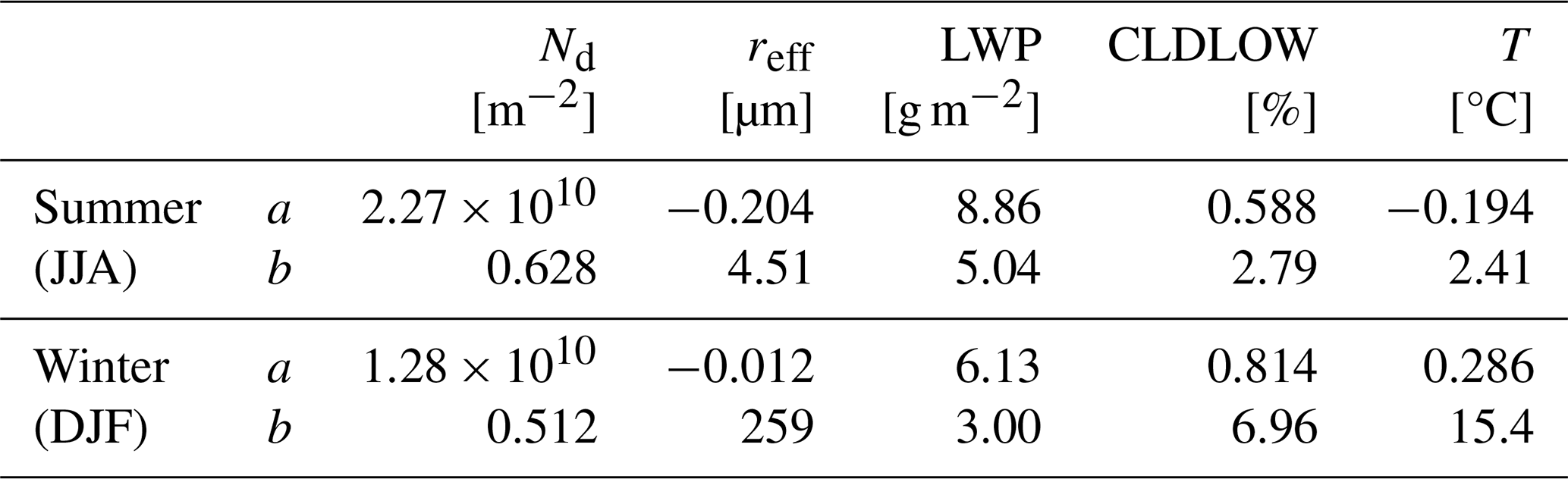
As discussed in Sect. 3.7, most anomalies gradually level off as the eruptions get larger. In other words, the magnitude of the climate response is sensitive to variations in eruption size for small eruptions but insensitive to such variations for large eruptions. To determine when this plateau is reached, we define a threshold for the growth rate provided in Eq. (5). Here, we choose a threshold value of a 1 % increase in absolute anomalies per scaling factor. This is a small, arbitrary number meant to indicate when the growth rate starts to level off, and it should be viewed as a guiding value rather than a hard separator. We consider eruptions resulting in a growth rate above this threshold (i.e. smaller eruptions) to be in the “sensitive stage”, while eruptions resulting in a growth rate below it (i.e. larger eruptions) are considered to have reached the “plateau stage”. Table 2 shows the magnitude scaling factors corresponding to the 1 % threshold. When comparing summer and winter, the 1 % threshold is generally reached for similarly sized eruptions. Surface air temperature is an exception as its growth rate decreases much more rapidly in winter. As for the cloud droplet effective radius during winter, the logarithmic fit does not offer much information since the mean Arctic anomalies remain constant as a function of eruption size. In most cases, the 1 % threshold is reached for scaling factors between × 20 and × 30. We would, therefore, expect the magnitude of the climate response to be more sensitive to the size of the eruption for eruptions smaller than about 20 times the size of the Holuhraun eruption and to be less sensitive to eruption size for eruptions larger than about 30 times this size. This applies to both summer and winter. The largest known effusive eruptions in Iceland were most likely around 20 times larger than the 2014–2015 Holuhraun eruption (see Sect. 1), and we would therefore expect them to have either reached or been close to reaching the plateau stage.

Table 2 Magnitude scaling factors for cases where the growth rate from Eq. (5) drops below 1 % per scaling factor with respect to the logarithmic fits (Eq. 4; based on the fitting coefficients from Table 1) for the variables given in Fig. 7, excluding SO₄ aerosols.

4.2 The 21st-century Fagradalsfjall fires

Within volcanology, the term “fires” refers to a single long-lasting volcanic eruption or a series of individual but connected eruptions. An example of the former is the 1784–1785 Laki eruption (also known as the Skaftá fires), and an example of the latter is the 1975–1984 Krafla fires, with both events occurring in Iceland. These fires typically last for years (Thordarson and Larsen, 2007). In 2021, a series of eruptions started on the Reykjanes Peninsula in Iceland. Collectively, these eruptions have not received an official name yet, but they are often referred to as the Fagradalsfjall fires. As of this writing, these fires are still ongoing.

The eruptions in the Fagradalsfjall fires share many similarities with the eruptions simulated in this study. They have all been effusive, their eruption plumes have mostly stayed below 3 km above sea level, and they have lasted between a few days and several months. The first eruption in the series, the 2021 Fagradalsfjall eruption, is the longest to date and lasted 6 months, from 19 March to 18 September 2021 (Pfeffer et al., 2024). Coincidentally, the 2014–2015 Holuhraun eruption also lasted 6 months, but it started in autumn (Gíslason et al., 2015). Holuhraun was, however, a much larger eruption, with estimated total SO₂ emissions of about 9.6 Tg (Pfeffer et al., 2018) compared to Fagradalsfjall's 0.97 Tg (Pfeffer et al., 2024). This gives the 2021 Fagradalsfjall eruption a magnitude scaling factor of about × 0.1 within the framework of our study.

Table 3 Estimated Arctic anomalies for a ×0.1-sized eruption using Eq. (4) and the simulations performed in this study. Spring corresponds to the March–May (MAM) mean for an eruption starting in March, summer corresponds to the June–August (JJA) mean for an eruption starting in June, autumn corresponds to the September–November (SON) mean for an eruption starting in September, and winter corresponds to the December–February (DJF) mean for an eruption starting in December. The numbers in brackets are the control means.

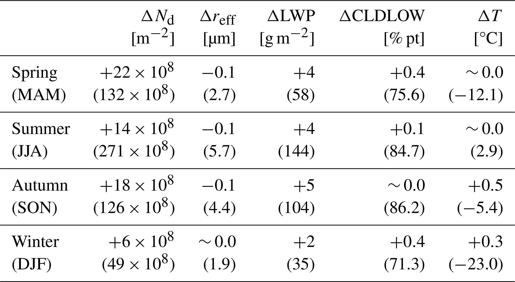
Table 3 lists the estimated Arctic anomalies for a × 0.1-sized eruption based on Eq. (4) and our simulations for the first 3 months of eruptions starting on the first days of March (spring), June (summer), September (autumn), and December (winter). Of these, the spring eruption most closely resembles the Fagradalsfjall eruptions in terms of starting date. These estimated anomalies for × 0.1-sized eruptions are very small and unlikely to stand out from natural variability. Other eruptions in the Fagradalsfjall fires have been much shorter, lasting only a few days or a few weeks (e.g. Esse et al., 2023; Sigmundsson et al., 2024), limiting their potential climate impacts due to the short lifetime of volcanic sulfur in the troposphere (e.g. Chin and Jacob, 1996; Schmidt and Carn, 2022). It is therefore unlikely that the Fagradalsfjall fires have caused significant climate impacts in the Arctic so far.

4.3 Observational evidence

The autumn of 2014 was warm over the Greenland Sea (e.g. in November in Ittoqqortoormiit, Jan Mayen, and Grímsey; Fig. A12b). Using observational and modelling evidence, Zoëga et al. (2023) argue that the 2014–2015 Holuhraun eruption contributed to this warming signal through increased cloud LW trapping under limited sunlight. Although the simulations performed for this study are not designed to exactly reproduce the 2014–2015 Holuhraun eruption (for example, with respect to the meteorology at the time), we nevertheless observe similarities in the climate response. When comparing anomalies from our x1sep simulations (which very closely resemble the 2014–2015 Holuhraun eruption in terms of emissions and timing), averaged over the Greenland Sea (approximated by the area between 65–80° N and 25° W–5° E), with anomalies from the ERA5 reanalysis for the same area, we find a warming signal in the autumn months of September to November in both cases (Fig. A12a). This, along with the results of Zoëga et al. (2023), lends support to the credibility of the high-latitude winter-warming mechanism discussed here.

4.4 Model dependencies

Aerosol–cloud interactions are among the largest sources of uncertainty in our understanding of the climate system, both from observational and modelling perspectives. This is especially true for the LWP and cloud fraction adjustments to aerosol perturbations (Forster et al., 2021). In a previous study, Malavelle et al. (2017) compared the cloud response to aerosol perturbations from the 2014–2015 Holuhraun eruptions across several different climate models. Among these models was CAM5, the predecessor of CAM6, which they found produced an overly strong LWP response over the open-ocean areas around Iceland compared to satellite retrievals. This result is further supported by a modelling study by Haghighatnasab et al. (2022), which found that neither the LWP nor the cloud cover response was attributable to this eruption. In contrast, recent studies using machine learning to analyse satellite data have found that the Holuhraun eruption did indeed lead to a significant increase in cloud fraction (Chen et al., 2022; Wang et al., 2024). Furthermore, analyses of both observational data (Zhao and Garrett, 2015) and satellite retrievals (Murray-Watson and Gryspeerdt, 2022) have found a positive relationship between the LWP and cloud droplet number concentration in the Arctic, which is where our simulations show the strongest increase in cloud LW trapping. The excessive LWP response in CAM5, reported by Malavelle et al. (2017), has since been addressed in CAM6 through modifications to the aerosol–cloud interaction processes, making the LWP less sensitive to perturbations in the cloud droplet number concentration (Gettelman and Morrison, 2015; Danabasoglu et al., 2020).

5 Conclusions

In this study, we use the Earth system model CESM2(CAM6) to systematically investigate the climate impacts of Northern Hemisphere, high-latitude, long-lasting effusive volcanic eruptions (similar to the 2014–2015 Holuhraun eruption in Iceland) as a function of eruption season and size. This systematic approach provides us with a broad view of the climate impacts of such eruptions and allows us to make quick estimates of the climate impacts of a wide range of effusive volcanic eruptions in Iceland. Our main results are twofold:

• The climate response to high-latitude, effusive volcanic eruptions is strongly modulated by different seasons. For winter eruptions, the model shows surface warming in the Arctic, and for summer eruptions, it shows surface cooling at midlatitudes and in the Arctic. The main contributors to this seasonal dependency are the availability of sunlight and atmospheric oxidants, Arctic sea ice cover, and background CCN and low-level cloud states.

• As eruptions increase in size in terms of SO₂ emissions, the magnitude of the climate response becomes less sensitive to variations in eruption size. In other words, the rate of change in the climate response as a function of eruption size is non-linear and decreases with increasing eruption size. For eruptions smaller than ca. 20 to 30 times the size of the 2014–2015 Holuhraun eruption, the magnitude of the climate response is highly sensitive to the size of the eruption. For larger eruptions, the climate response becomes saturated, displaying only minor variations with increased SO₂ emissions.

When the climate impacts of effusive volcanic eruptions are discussed, the focus is usually on cooling effects due to increased reflectance of sunlight (e.g. Eguchi et al., 2011; Schmidt et al., 2012; Malavelle et al., 2017). However, we have evidence for the opposite – namely, significant warming in the Arctic during the early winter as a result of a long-lasting effusive volcanic eruption (Zoëga et al., 2023). In this study, we have illustrated how sensitive the climate response to such eruptions is to the season of the eruption and how surface warming is the dominant response at high latitudes during winter. The idea that effusive volcanic eruptions lead to surface cooling is therefore an oversimplification according to our results, especially in the Arctic.

In light of the high effusive volcanic activity in Iceland, especially over the past decade (e.g. the 2014–2015 Holuhraun eruption and the ongoing Fagradalsfjall fires on the Reykjanes Peninsula); the potential for very large eruptions (e.g. the 1783–1784 Laki eruption and the 939–940 Eldgjá eruption); the rapidly changing climate in the Arctic; and the similarities to cloud-seeding geoengineering, understanding the climate impacts of high-latitude, effusive volcanic eruptions becomes increasingly relevant.

Appendix A

A1 Background aerosol and cloud conditions

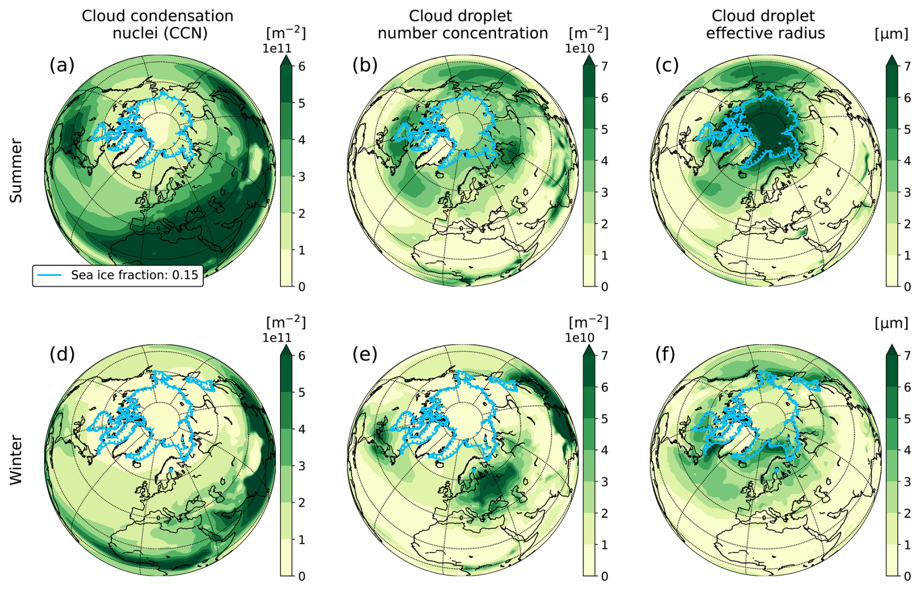
Figure A1 Summer (June–August) and winter (December–February) means from the CESM2(CAM6) control run for cloud condensation nuclei (a, d), cloud droplet number concentration (b, e), and the cloud droplet effective radius (c, f).

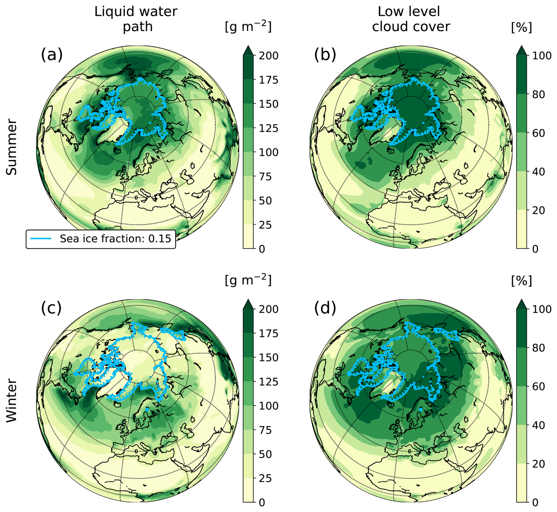
Figure A2 As in Fig. A1 but for the liquid water path (a, c) and low-level cloud cover (b, d).

A2 Precipitation

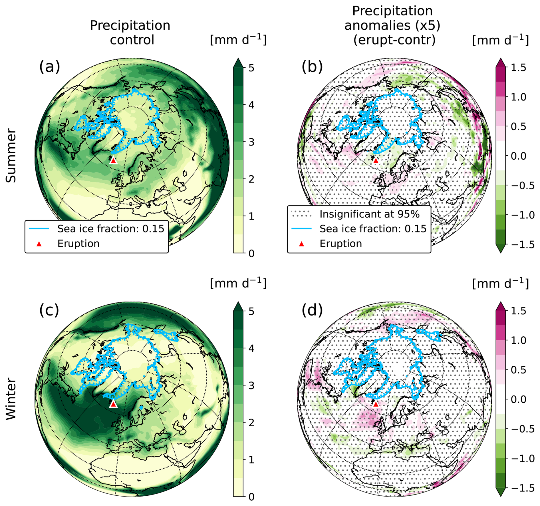
Figure A3 Precipitation from the CESM2(CAM6) simulations. Control means for (a) summer (June to August) and (c) winter (December to February). Mean anomalies for the first 3 months of the eruption for the (b) x5jun and (d) x5dec scenarios.

A3 Vertical profiles

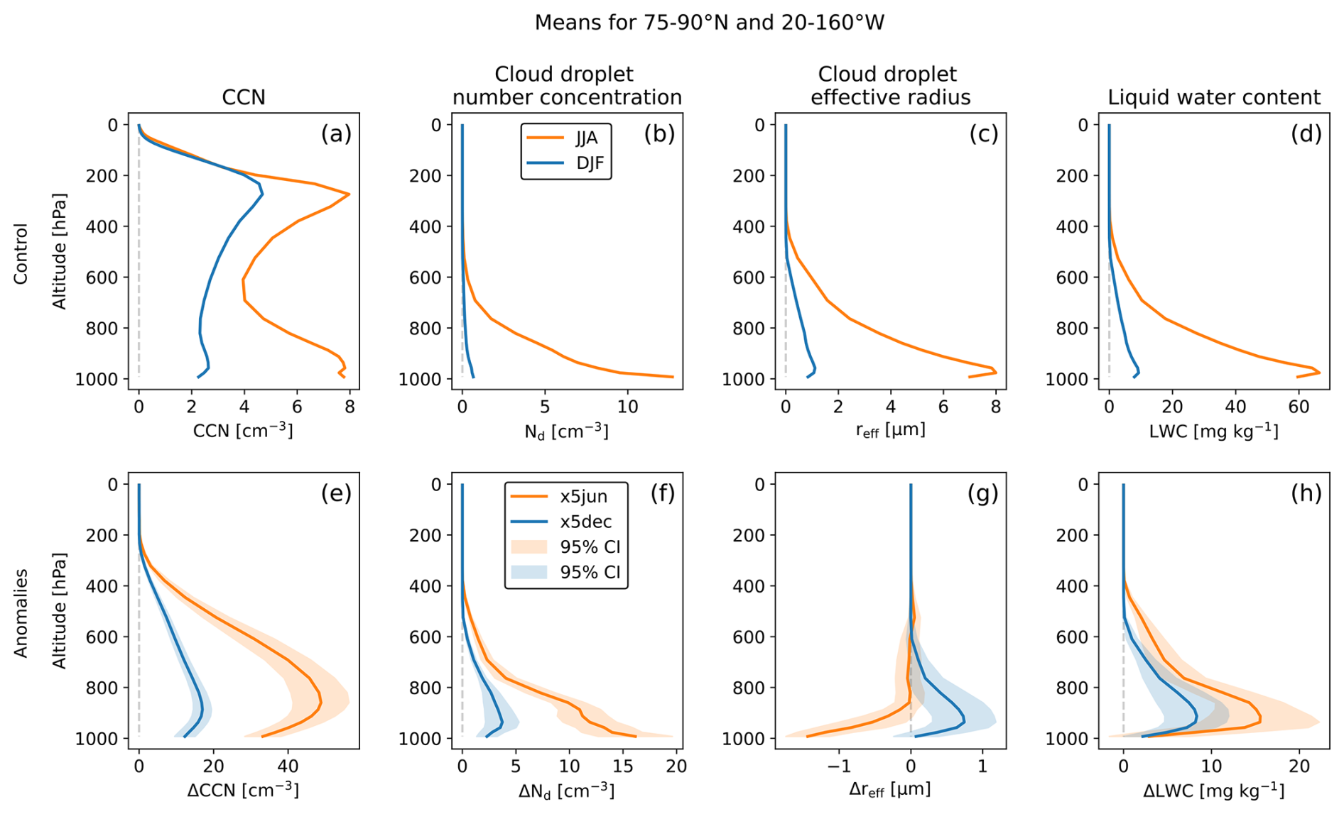
Figure A4 Vertical profiles for mean summer (June–August) and winter (December–February) background conditions from the control run are shown in the top row (a–d), and mean anomalies for the first 3 months of the x5jun and x5dec eruption scenarios are shown in the bottom row (e–h). Means are calculated over Arctic sea ice, bounded by 75–90° N and 20–160° W. Profiles are shown for cloud condensation nuclei (a, e), cloud droplet number concentration (b, f), the cloud droplet effective radius (c, g), and liquid water content (LWC) (d, h).

Figure A5 As in Fig. A4 but for relative humidity (RELHUM) (a, d), sub-grid vertical velocity (WSUB) (b, e), and lapse rate (LR) (c, f).

A4 Direct aerosol effects

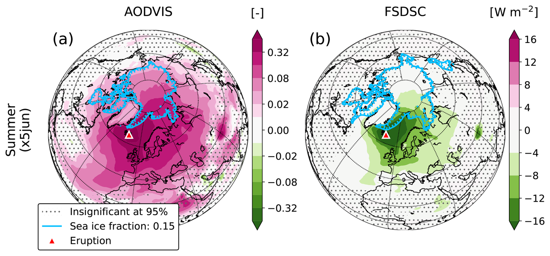
Figure A6 Mean anomalies for the first 3 months of the eruption for the x5jun scenarios for (a) aerosol optical depth at 550 nm (in the visible part of the electromagnetic spectrum, AODVIS) and (b) downward clear-sky SW flux at the surface (FSDSC).

A5 Surface albedo

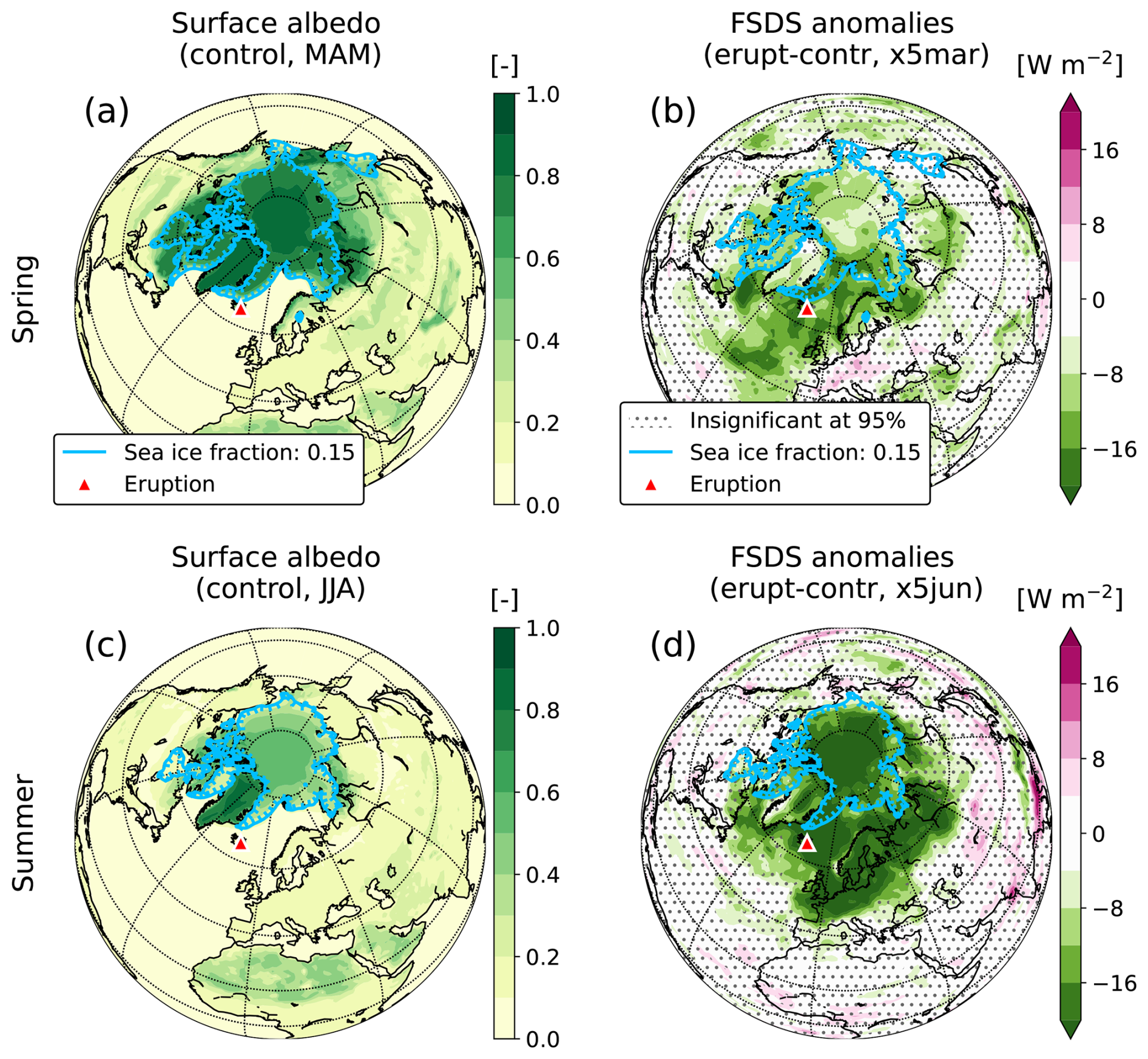
Figure A7 Surface albedo means from the control run for (a) spring (March to May) and (c) summer (June to August). Mean anomalies for surface downward shortwave radiation (FSDS) for the first 3 months of the (b) x5mar and (d)​​​​​​​ x5jun simulations.

A6 Sea surface temperature and sea ice cover

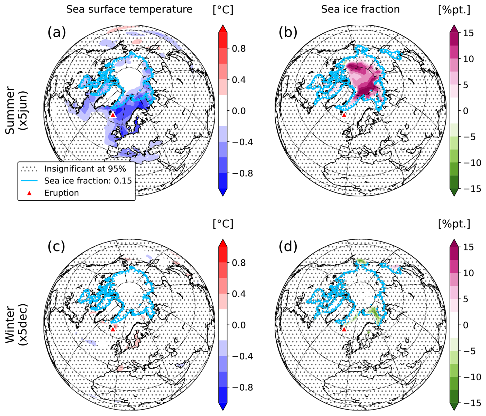
Figure A8 As in Fig. 2 but for sea surface temperature (a, c) and sea ice fraction (b, d).

A7 The North Atlantic Oscillation

We calculate the North Atlantic Oscillation (NAO) index from our model data as the difference in normalized sea-level pressure between the Azores (38.2° N, 27.0° W) and Stykkishólmur, Iceland (65.1° N, 22.7° W), i.e.

$$\begin{array}{}\text{(A1)}& {\mathrm{NAO}}_{\mathrm{ind}}=P_{\mathrm{Az}}^{\prime }-P_{\mathrm{St}}^{\prime },\end{array}$$

where $P_{\mathrm{Az}}^{\prime }$ and $P_{\mathrm{St}}^{\prime }$ are the normalized sea-level pressures for the Azores and Stykkishólmur, respectively, and

$$\begin{array}{}\text{(A2)}& P^{\prime }={\displaystyle \frac{P-\stackrel{\mathrm{‾}}{P}}{{\mathit{\sigma }}_P}},\end{array}$$

where $\stackrel{\mathrm{‾}}{P}$ and σ_P are the mean sea-level pressure and standard deviation from the control run, respectively.

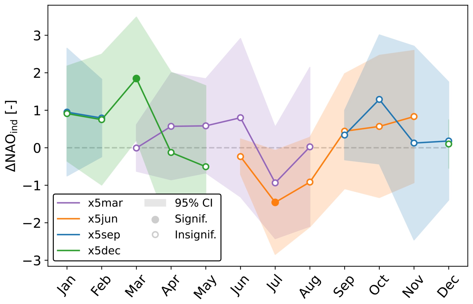
Figure A9 Modelled monthly mean North Atlantic Oscillation (NAO) index anomalies for eruptions using the × 5 scaling factor. The NAO index is calculated as the difference in normalized sea-level pressure between the Azores and Stykkishólmur, Iceland.

A8 Spring and autumn

Figure A10 As in Fig. 7 but for eruptions starting in March (green) and September (purple).

A9 Sea-level pressure

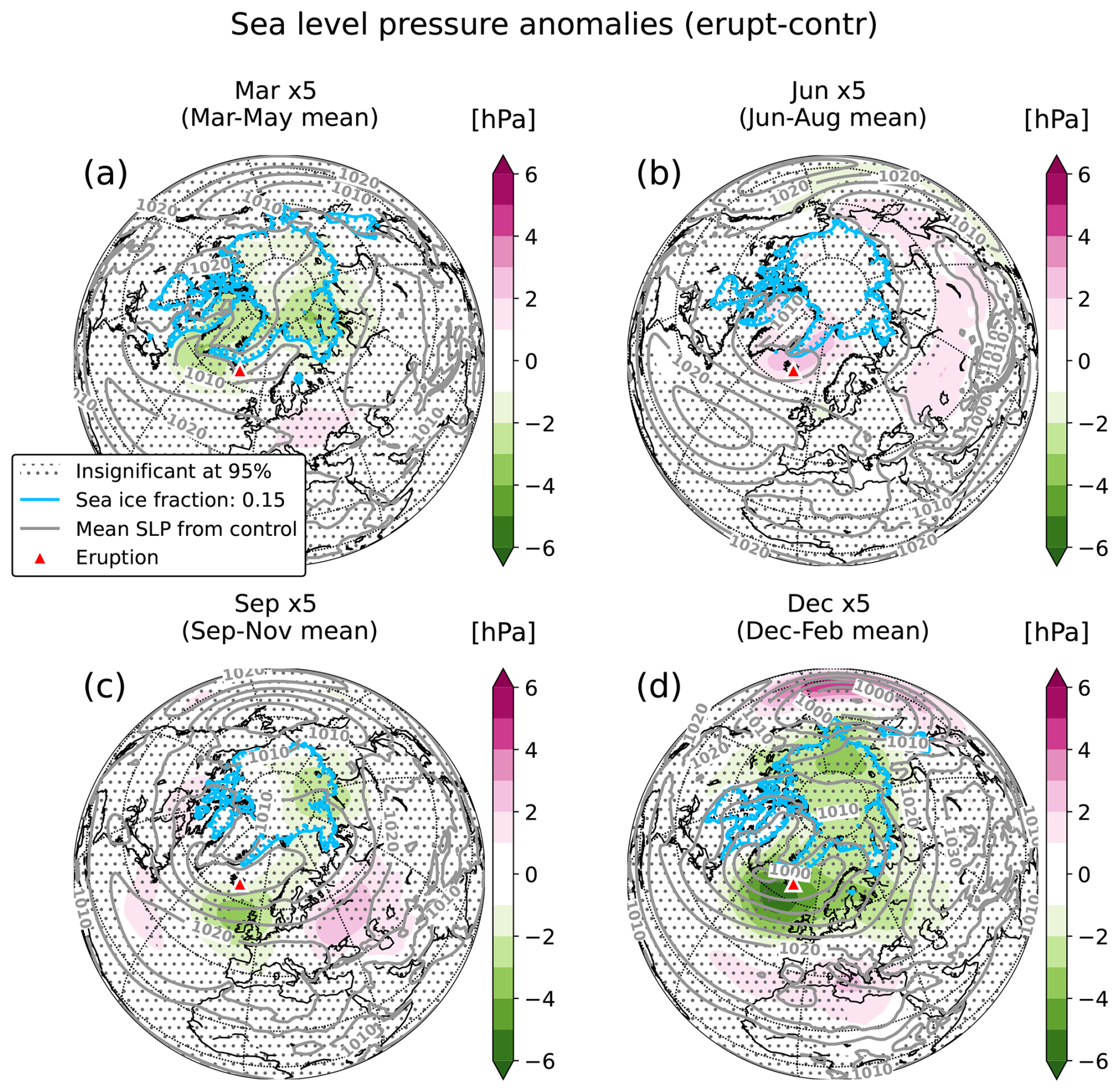
Figure A11 Sea-level pressure (SLP) anomalies for the first 3 months of an eruption for the (a) x5mar, (b) x5jun, (c) x5sep, and (d) x5dec scenarios. The grey contours represent control means.

A10 Observational evidence: comparing the 2014–2015 Holuhraun eruption and the x1sep simulations

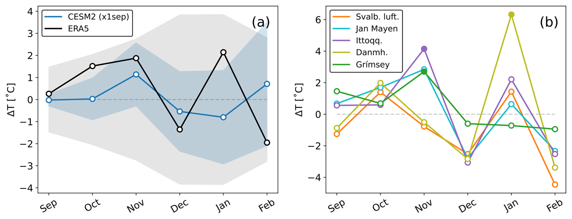
Figure A12 (a) Monthly mean surface air temperature anomalies averaged over the Greenland Sea, defined by the area between 66–80° N and 25° W–5° E. The blue line shows the x1sep CESM2(CAM6) ensemble mean anomalies. The black line represents anomalies from September 2014 to February 2015, relative to the 1984–2013 (30-year) climatology from the ERA5 reanalysis. Shading indicates the 95 % confidence interval for the CESM2(CAM6) simulations and the 95 % prediction interval for ERA5. (b) Observed monthly mean surface air temperature anomalies from stations in and around the Greenland Sea: Svalbard Airport (Svalb. luft.) (78.25° N, 15.50° E; orange), Jan Mayen (70.94° N, 8.67° W; cyan), Ittoqqortoormiit (Ittoqq.) (70.48° N, 21.95° W; purple), Danmarkshavn (Danmh.) (76.77° N, 18.68° W; olive), and Grímsey (66.54° N, 18.02° W; green). Anomalies are from September 2014 to February 2015 and are relative to the 1984–2013 climatology. Prediction intervals are not plotted to maintain clarity. For all time series in both panels (a) and (b), filled dots indicate significant anomalies, while unfilled dots represent insignificant anomalies.