the Creative Commons Attribution 4.0 License.
the Creative Commons Attribution 4.0 License.
 | 10 Mar 2025
Ozone trends in homogenized Umkehr, ozonesonde, and COH overpass records
Irina Petropavlovskikh
Jeannette D. Wild
Kari Abromitis
Peter Effertz
Koji Miyagawa
Lawrence E. Flynn
Eliane Maillard Barras
Robert Damadeo
Glen McConville
Bryan Johnson
Patrick Cullis
Sophie Godin-Beekmann
Gerard Ancellet
Richard Querel
Roeland Van Malderen
Daniel Zawada
This study presents an updated evaluation of stratospheric ozone profile trends at Arosa/Davos/Hohenpeißenberg, Switzerland/Germany; Observatory de Haute-Provence (OHP), France; Boulder, Colorado, Mauna Loa Observatory (MLO) and Hilo, Hawaii; and Lauder, Aotearoa / New Zealand, with a focus on the ozone recovery period post-2000. Trends are derived using vertical ozone profiles from NOAA's Dobson network via the Umkehr method (with a recent new homogenization), ozonesondes, and the NOAA COHesive Solar Backscatter Ultraviolet Instrument (SBUV)/Ozone Mapping and Profiler Suite (OMPS) satellite-based record (COH) sampled to match the geographical coordinates of the ground-based stations used in this study. Analyses of long-term changes in stratospheric ozone time series were performed using the updated version (0.8.0) of the Long-term Ozone Trends and Uncertainties in the Stratosphere (LOTUS) independent linear trend (ILT) regression model. This study finds consistency between the trends derived from the different observational records, which is a key factor to the understanding of the recovery of the ozone layer after the implementation of the Montreal Protocol and its amendments that control ozone-depleting substance production and release into the atmosphere. The northern hemispheric Umkehr records of Arosa/Davos, OHP, and MLO all show positive trends in the mid- to upper stratosphere, with trends peaking at ∼ +2 % per decade. Although the upper-stratospheric ozone trends derived from COH satellite records are more positive than those detected by the Umkehr system, the agreement is within the 2 times the standard error uncertainty. Umkehr trends in the upper stratosphere at Boulder and Lauder are positive but not statistically significant, while COH trends are larger and statistically significant (within 2 times the standard error uncertainty). In the lower stratosphere, trends derived from Umkehr and ozonesonde records are mostly negative (except for positive ozonesonde trends at OHP); however, the uncertainties are quite large. Additional dynamical proxies were investigated in the LOTUS model at five ground-based sites. The use of additional proxies did not significantly change trends, but the equivalent latitude reduced the uncertainty in the Umkehr and COH trends in the upper stratosphere and at higher latitudes. In lower layers, additional predictors (tropopause pressure for all stations; two extra components of Quasi-Biennial Oscillation at MLO; Arctic Oscillation at Arosa/Davos, OHP, and MLO) improve the model fit and reduce trend uncertainties as seen by Umkehr and sonde.
- Article
(13584 KB) - Full-text XML
- BibTeX
- EndNote


The World Meteorological Organization (WMO) Ozone Assessments (WMO, 2018, 2022), indicate that for some geographical regions, the stratospheric ozone layer is recovering in accordance with the reduction in the ozone-depleting substances (ODSs) whose production was restricted by the Montreal Protocol and its amendments. The U.S. Clean Air Act requires NOAA to monitor prohibited chemicals and the ozone layer to ensure the success of the Montreal Protocol. NOAA's long-term network of measurements helps to interpret total column and vertically resolved ozone changes and link ozone recovery to the reduction in ODS levels in the stratosphere, changes in the lower stratosphere that are associated with climate changes, and increases in the troposphere that are influenced by the stratosphere–troposphere exchange and long-range transported pollution. The ongoing recovery of the stratospheric ozone layer is of great importance to human health (i.e., cancer from enhanced UV exposure; Madronich et al., 2021), the sustained production of crops, and the success of fisheries (dangerous algae blooms). For more information, see the Environmental Effects Assessment Panel 2022 Quadrennial Assessment (EEAP, 2023).
The Long-term Ozone Trends and Uncertainties in the Stratosphere (LOTUS) study was initiated under Stratosphere–troposphere Processes And their Role in Climate (SPARC; changed to APARC in 2024) project to reconcile the differences in defining trend uncertainties between methods outlined in the WMO Assessment (WMO, 2014) and the SPARC/IO3C/IGACO-O3/NDACC (SI2N) study (Harris et al., 2015). Phase 1 focused on developing best practices for data merging, trend determination, and error analyses. Results focused on the analysis of broad latitudinal regions that are near-global, namely the Northern Hemisphere, Southern Hemisphere, and tropics, as used in the SI2N studies. Results are found in the 2019 report (Petropavlovskikh et al., 2019). Phase 2 refined the trend models and extended the study to gridded and ground-based (GB) ozone datasets. The development of the methods used in trend detection is built on the community knowledge gained during the Tiger Team project in early 1990s (Reinsel et al., 2005); collaborations through the SPARC-, WMO-, and IO3C-supported LOTUS activity (Hassler et al., 2014; Harris et al., 2015; Godin-Beekmann et al., 2022); and the most recent contributions to the WMO Ozone assessment analyses published in Chap. 3, “Update on Global Ozone: Past, Present and Future” (Hassler et al., 2022).
Understanding the causes of the differences between GB and satellite records can create improvements not only in the internal consistency of datasets but also in the uncertainties in overall ozone trends. Furthermore, the development of techniques to directly assess uncertainties in the merged records resulting from discrepancies that cannot be completely reconciled, such as small relative drifts and differences resulting from coordinate transformations and sampling differences, allows for a more precise estimate of the significance of the mean trends. For the GB and satellite data used in the 2019 LOTUS report, information on the stability and drifts of the measurement was incomplete. The homogenization of many ozonesonde records was recently addressed, and data were reprocessed (Tarasick et al., 2016; Van Malderen et al., 2016; Witte et al., 2017; Sterling et al., 2018; Witte et al., 2018; Ancellet et al., 2022), while some instrumental artifacts still need to be addressed (Smit et al., 2021).
The first attempt to evaluate representativeness of the trends derived from GB station records in the middle and upper stratosphere using Solar Backscatter Ultraviolet Instrument (SBUV) data was done as a part of the LOTUS activity and was discussed in the 2019 LOTUS report. Comparisons of trends derived from satellite data sub-sampled at the station location (overpass) to those derived from the relevant zonal average provide a measure of potential sampling errors when comparing satellite and GB trends (Zerefos et al., 2018; Godin-Beekmann et al., 2022). This paper continues that work by comparing trends derived from several GB and satellite records that are matched spatially. We further investigate the impact of temporal matching on trends.
The common statistical linear regression trend model used in the 2019 LOTUS report and the 2022 update (Godin-Beekmann et al., 2022) was optimized for analyses of the zonally averaged satellite datasets. However, analyses of the GB and satellite overpass ozone profile data may require a reconsideration of additional proxies and optimization methods to improve the interpretation of the processes that impact ozone changes over limited geophysical regions and reduce trend uncertainties. An assessment of model sensitivities to uncertainties in the volcanic aerosols, solar cycle, Quasi-Biennial Oscillation (QBO), El Niño–Southern Oscillation (ENSO), and other mechanisms also need to be considered in the GB and satellite overpass record trend analysis. The localized time series for the assessment of dynamical and chemical proxies can improve the attribution of ozone variability, especially in the lower stratosphere, thus reducing uncertainties in the derived trends. This paper provides an assessment of uncertainties in the derived trends from the NOAA ground-based, ozonesonde, and SBUV/Ozone Mapping and Profiler Suite (OMPS) (zonally averaged and overpass) records and reports improvements in the multiple linear regression (MLR) trend uncertainties with the addition of proxies representing interannual dynamical variability or long-term changes in atmospheric circulation. The ability of the ground-based and ozonesonde records to capture semi-global ozone changes is evaluated by comparing trends derived from the satellite overpass and zonally averaged records.
In the LOTUS report, the ozone trends were analyzed at low and middle latitudes, with a focus on the upper and middle stratosphere. This paper includes middle- and low-latitude trends assessed in the lower stratosphere and thus offers an opportunity to test the additional proxy for the tropopause pressure (Thompson et al., 2021).
2.1 Umkehr and ozonesonde records at NOAA
The Dobson ozone spectrophotometer has been used to study total ozone since its development in the 1920s (Staehelin et al., 2018). Dobson records are regularly used in satellite record validation (Bai et al., 2015; Koukouli et al., 2016; Boynard et al., 2018) and the development of global combined ozone data records (Fioletov et al., 2008; Hassler et al., 2018). The NOAA Dobson ozone record was homogenized in 2017 to account for inconsistencies in the past calibration records, data processing methods, and selection of representative data (Evans et al., 2017). NOAA Dobson instruments at four stations and MeteoSwiss at Arosa/Davos also measure Umkehr profiles, which are derived as partial column ozone amounts in ∼ 5 km layers. Profiles are derived using an optimum statistical inversion of Dobson measurements taken continuously at different solar zenith angles (SZAs) (Petropavlovskikh et al., 2005; Hassler et al., 2014). These Umkehr data were recently homogenized to assure the removal of small but significant instrumental artifacts that can impact the accurate detection of stratospheric ozone trends (Petropavlovskikh et al., 2022; Maillard Barras et al., 2022). This study focuses on Umkehr records from the MeteoSwiss station of Arosa/Davos, Switzerland, and on Umkehr records from the NOAA stations of Boulder, Colorado; Mauna Loa Observatory (MLO), Hawaii; Lauder, Aotearoa / New Zealand; and the Umkehr record from Observatory de Haute-Provence (OHP), France. NOAA-GML (NOAA Global Monitoring Laboratory) for Umkehr data means that the NOAA optimization process was applied to the operational records (N values) prior to the retrieval of ozone profiles. The source data used in this study are available at https://doi.org/10.15138/1FF4-HC74 (Miyagawa et al., 2024). See Table 1 for details on the GB datasets, locations, source of data, and temporal extent of data used. Umkehr measurements are typically made twice per day when there is no cloud obstruction.
Table 1GB datasets, location, instrument type, temporal extent, and data record source. For the trend calculations, we remove data during volcanic periods from 1982–1984 and 1991–1994. WOUDC stands for World Ozone and Ultraviolet Radiation Data Centre.
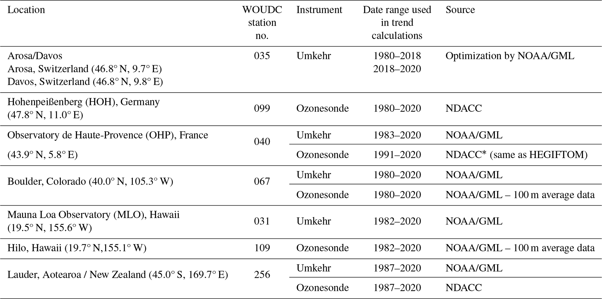
* Note that data from the “corrected ozone partial pressure” column are used for trend analyses.
The ozonesonde instrument has been flown at four NOAA stations since the 1980s. Evolving instrumentation and standard operating procedures led to the development of data homogenization methods by NOAA and the international community (i.e., ASOPOS-1 (Assessment of Standard Operating Procedures for OzoneSondes); Smit and the ASOPOS panel, 2014) to resolve record inconsistencies in the NOAA (Sterling et al., 2018), Canadian (Tarasick et al., 2016), and SHADOZ (Southern Hemisphere ADditional OZonesondes) networks (Witte et al., 2017, 2018). The effort was extended in the ASOPOS-2 (Smit et al., 2021) activity and included a larger group of stations that are part of the NDACC (Network for Detection of Atmospheric Composition Change) and WMO GAW (World Meteorological Organization Global Atmosphere Watch program) networks. The error budget for each profile is calculated and included in the archived files (Sterling et al., 2018). Modern ozonesonde instruments measure ozone at a high vertical resolution on the order of 100 m (Thompson et al., 2019), depending on the balloon accent velocity and the time response of the instrument.
The sondes constitute an essential component of satellite calibration and cross-calibration (Hubert et al., 2016), verification, and improvement of climate chemistry and chemistry transport models (Wargan et al., 2018; Stauffer et al., 2019). The Dobson total ozone, Umkehr, and ozonesonde profile records provide key measurements for upper- and middle-stratospheric ozone trend calculations and are part of the NOAA benchmark network for stratospheric ozone profile observations (Petropavlovskikh et al., 2019; Godin-Beekmann et al., 2022; WMO, 2022).
The ozonesonde data are used for trend analyses from the OHP, Boulder, and Lauder stations for which we have Umkehr observations. Ozonesondes are launched at Hilo, Hawaii, which is nearly co-located with MLO. Ozonesonde data for the Arosa/Davos panel are selected from the Hohenpeißenberg (HOH), Germany, station that is in close vicinity to Arosa/Davos station. Sonde measurements are typically measured once or twice per week, varying somewhat with station operational procedures.
Data for the NOAA GML ozonesonde records are publicly available from the NOAA Global Monitoring Lab (GML) at https://gml.noaa.gov/aftp/data/ozwv/Ozonesonde/ (last access: 1 June 2024). We use the “100 meter average files” in each station directory. Other sonde datasets used in this study are also available from several other data centers, including the World Ozone and Ultraviolet Radiation Data Centre (WOUDC; https://woudc.org/, last access: 1 June 2024), the Network for the Detection of Atmospheric Composition Change (NDACC; https://www.ndacc.org, last access: 1 June 2024) data centers, or the Harmonization and Evaluation of Ground-based Instruments for Free-Tropospheric Ozone Measurements (HEGIFTOM; https://hegiftom.meteo.be/, last access: 1 June 2024) archive. Table 1 denotes the source of each dataset used in this study.
The ozonesonde data are of significantly higher vertical resolution (even when used as 100 m averages) than the Umkehr data layers of approximately 5000 m. In order to create a dataset with comparable resolution, we use the Umkehr averaging kernels (AKs) to smooth the sonde data. Details appear in Appendix A. We cap the sonde profile at Umkehr layer 5 (16–32 hPa) as there is not sufficient sonde information at higher altitudes to meet the requirements of the AKs for layers 6 and above. We further match the ozonesonde data to the dates when both Umkehr and sonde data are available, using ±24 h to find a match, and then generate the ozonesonde monthly mean. Appendix D explores the impact of temporal sampling on trends. The final matched dataset, with AK averaging, is publicly available at https://doi.org/10.15138/1FF4-HC74 (Miyagawa et al., 2024).
2.2 The NOAA Cohesive (COH) station overpass ozone profile datasets
NASA and NOAA have produced satellite measurements of ozone profiles through the Solar Backscatter Ultraviolet Instrument (SBUV) on the sequence of Polar Operational Environmental Satellites (POES) since 1978. This measurement series is extended with the related Ozone Mapping and Profiler Suite (OMPS) nadir profiler (NP) instruments using similar measurement techniques and retrieval algorithms. These combine to provide nearly 45 years of continuous data (1978–present). This single-instrument-type dataset eliminates many homogeneity issues, including varying vertical resolution or instrumentation differences. Version 8.6 SBUV data incorporate additional calibration adjustments beyond the version 8 release (McPeters et al., 2013). Small but evident biases remain (Kramarova et al., 2013a). Several methods have been historically used to combine these datasets into a continuous series. The NASA MOD version 1 dataset based on SBUV and OMPS v8.6 (Frith et al., 2014) combines data from all available satellites with no modification or bias adjustments. NASA has developed an alternate processing for the SBUV and OMPS data (v8.7) that incorporates new calibrations at the radiance level and has updated a priori with improved troposphere. Additionally, the a priori is chosen to be representative of the local solar time of the measurement. MOD v2 is based on the v8.7 processing (Frith et al., 2020) and further applies an adjustment to the v8.7 data to shift all measurements to a nominal measurement time of 13:30 local time.
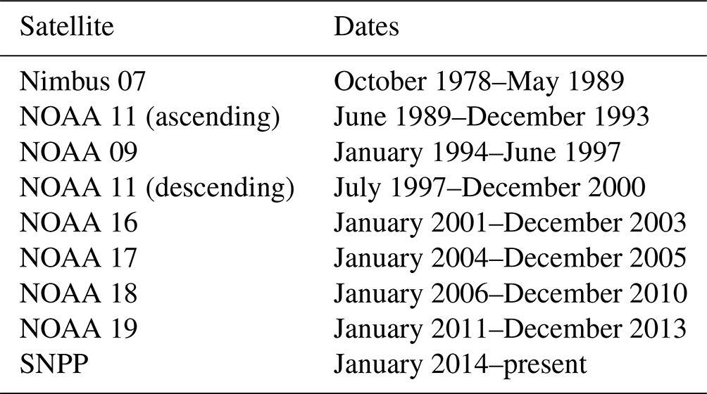
The NOAA SBUV/2 and OMPS Cohesive dataset (hereafter referred to as COH) combines data from the SBUV/2 and OMPS instruments using NASA's version 8.6 for the SBUV/2 data and NOAA/National Environmental Satellite, Data, and Information Service (NESDIS) version 4r1 for the OMPS Suomi National Polar-orbiting Partnership (SNPP) data. This dataset uses correlation-based adjustments providing an overall bias adjustment plus an ozone-dependent factor (Wild et al., 2016) to moderate the remaining biases between instruments in the series. The resulting profile product is a set of daily or monthly zonal means and is publicly available at https://ftp.cpc.ncep.noaa.gov/SBUV_CDR (last access: 1 June 2024). Zones are 5° wide in latitude as identified by the central latitude (2.5°, 7.5°, etc.). Contributing satellites and their period of use are shown in Table 2.
A previous version of this dataset using OMPS v3r2 has been used in climate reviews and trend studies (Godin-Beekmann et al., 2022; Weber et al., 2022a, b) including Chap. 3 of the WMO Ozone Assessment (Hassler et al., 2022). Appendix B examines the differences between the data versions. The impact on trends is limited to less than 1 % per decade, which is well within the precision of the trend results.
We create the overpass data at a ground station by collecting all profiles from a satellite within a ° latitude/longitude box centered on the station. The box size is chosen to ensure that one to four points are found per day. Fewer points are found if the orbit passes directly over the station; more points are found if the orbits straddle the station. The collected profiles are inverse-distance-weighted to the station location and averaged. COH style adjustments are applied (Wild et al., 2016), creating a COH overpass time series from 1978 to the present. This dataset is available on the NOAA website at https://ftp.cpc.ncep.noaa.gov/SBUV_CDR/overpass (last access: 1 June 2024).
Figure 1 shows the ozone anomaly time series for the 40–45° N zonal average data and for the data at three stations in or near the zone. Anomalies are calculated with respect to the zonal average climatology. The series shown are for the layer data, with the bottom pressure of the layer displayed on the right side of the graph. This depiction retains the information about the relative differences between the stations and the zonal average. In the mid-stratosphere (25–10 hPa), the biases between the stations are most pronounced, with Arosa/Davos usually showing less ozone and Boulder usually showing more ozone. At the uppermost layers (1 and 4 hPa) and the lowest layer (41 hPa), the bias between stations is reduced. The anomalies for Arosa/Davos and OHP, which are geographically closer than Boulder, are often nearly anticorrelated with the Boulder anomalies, especially in the second half of the year. Indeed, at 16 hPa in particular, one can see that often the Boulder anomalies are positive when the Arosa/Davos and OHP anomalies are negative.
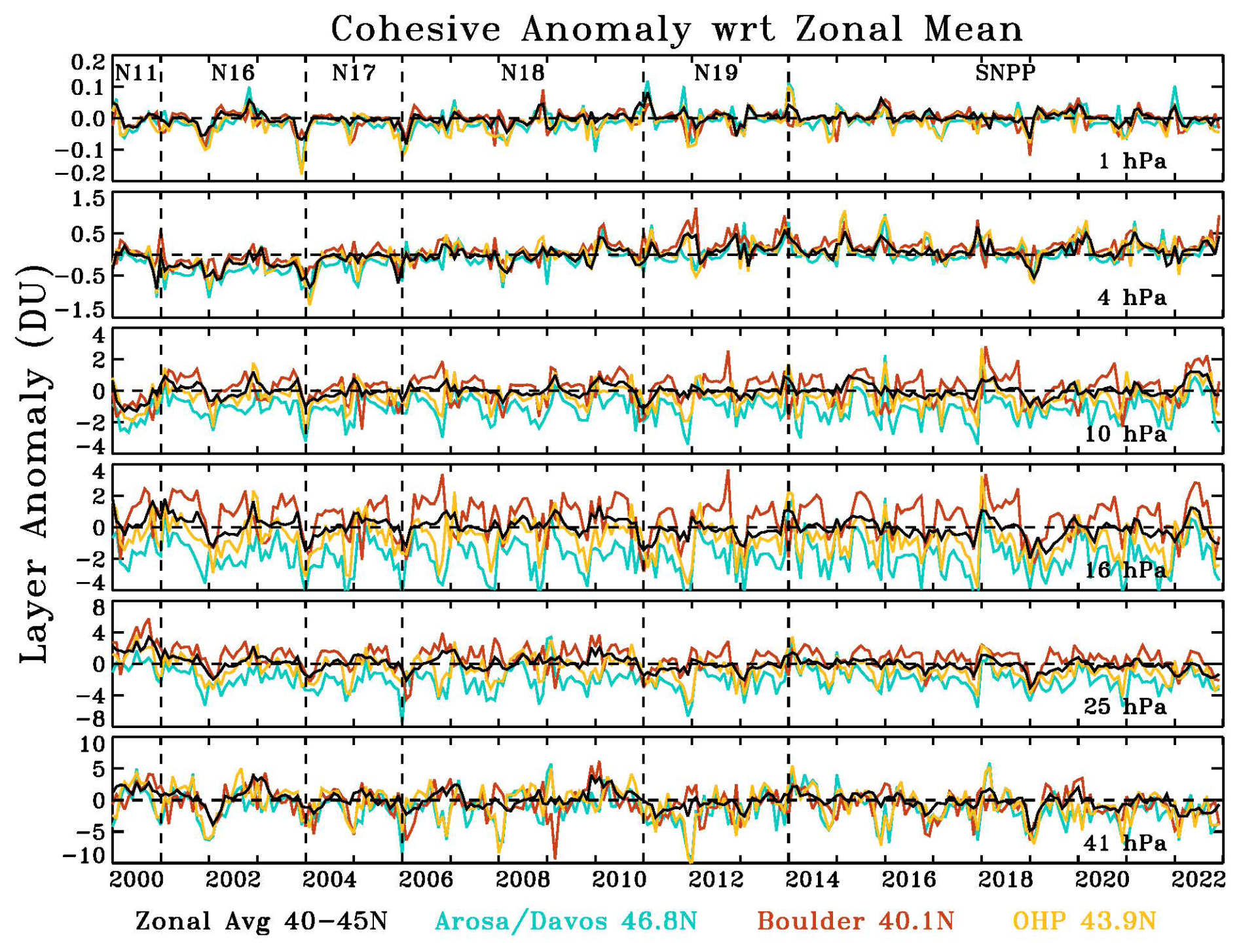
Figure 1Monthly ozone anomaly relative to the zonal mean monthly averages. This process leaves intact the trend for each site and the zone and accentuates the differences between the station values since all anomalies are referenced to the zonal product. Evident at 4 hPa is a positive trend from 2002 to 2013 and then a leveling out thereafter.
Figure 2 also shows the anomalies for the 40–45° N zonal average with the station anomalies, but each anomaly is now created using the climatology derived from each separate dataset. This removes the bias between the stations and the zones. At 1 hPa, Arosa/Davos appears to display the most variation (largest peaks and dips) in the anomalies. Since the anomaly for each site is now based on the seasonality of each site's data, the structure of the anomalies is more uniform. For example, now at 16 hPa, the difference between Boulder and the two sites Arosa/Davos and OHP in the latter half of the year is removed. In 2012, where the Boulder anomaly was positive with respect to the zonal average seasonal value, and the Arosa/Davos and OHP sets were negative with respect to the zonal seasonal average, all of them are now of the same sign with respect to their own seasonal averages. Nonetheless, there are events for which one station shows the opposite anomalies to the other two, for example, in early 2009 at 41 hPa, when the Boulder anomaly is negative, and Arosa/Davos and OHP are positive. Thus, it is noted that when comparing daily or monthly data values from GB and satellite data, the overpass data will reveal a different structure to the zonal data. The trend calculations in this paper are based on the datasets of Fig. 2, where the seasonal behavior is removed using the station seasonality.
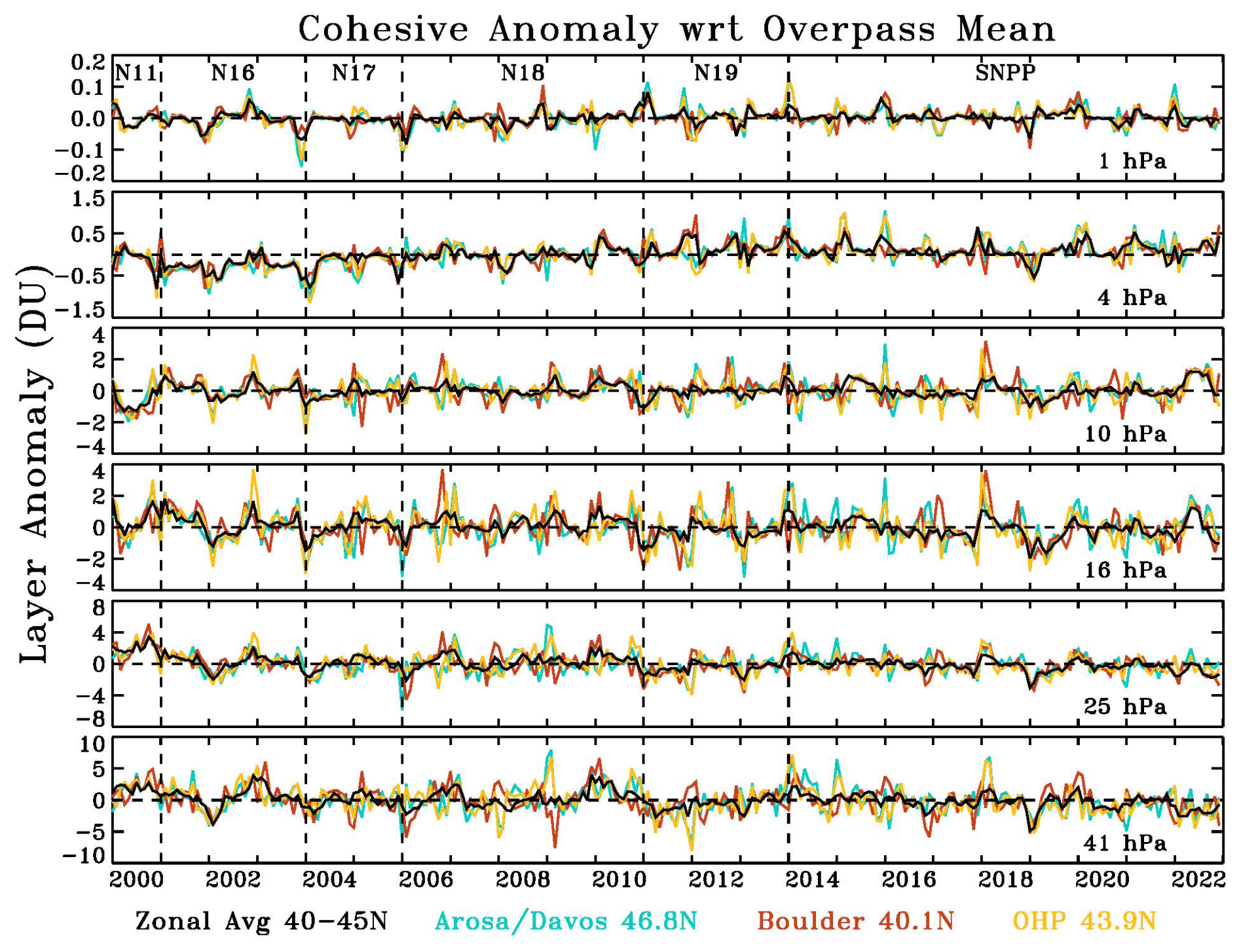
Figure 2Monthly ozone anomaly relative to the monthly climatology for each station overpass dataset. This process leaves intact the trend for each site and the zone and shows the consistency among the stations when each station climatology is removed. This dataset is used for the trend calculations. Evident at 4 hPa is a positive trend from 2002 to 2013 and then a leveling out thereafter. Trends are run on this dataset.
The COH overpass and zonal datasets have a similar vertical granularity to the Umkehr dataset but use somewhat different pressures for the demarcation of the top and bottom of each layer. Since no additional smoothing is required, we simply use interpolation and integration to convert the COH layer profiles to the Umkehr layers. We exclude layers 1 to 4 since there is little sensitivity in SBUV and OMPS NP in these layers (Kramarova et al., 2013b). The overpass monthly mean dataset in this study uses all COH data matched to dates when Umkehr data also exists. This dataset is publicly available at https://doi.org/10.15138/1FF4-HC74 (Miyagawa et al., 2024). Appendix D explores the impact of temporal sampling on trends.
This study also uses a specialized zonal monthly mean COH product which is the average of all daily profiles with an Umkehr match at the associated GB station. Zones used for most stations are the 5° wide zone that includes the geographic station latitude (Arosa/Davies: 47.5° N; OHP: 42.5° N; MLO: 17.5° N). Boulder and Lauder, however, are located directly on the border of two zones, so the zonal product in this study is the mathematical average of the two adjacent zones (Boulder: 37.5 and 42.5° N; Lauder: 42.5 and 47.5° S).
3.1 LOTUS model overview – the reference model
The Long-term Ozone Trends and Uncertainties in the Stratosphere (LOTUS) activity is a project of SPARC (Stratosphere–troposphere Processes And their Role in Climate) and has produced a statistical multiple linear regression (MLR) model called the LOTUS model (https://usask-arg.github.io/lotus-regression/index.html, last access: 1 June 2024).
The 2019 LOTUS report (Petropavlovskikh et al., 2019) and update (Godin-Beekmann et al., 2022) have quantified stratospheric ozone trends and evaluated their uncertainties. The LOTUS model is a general least squares approach MLR model. This study uses version l (v 0.8.0) with the independent linear trend (ILT) configuration. The independent linear terms represent the ozone depletion period (pre-1997), the ozone recovery period (post-2000), and an optional gap period (1997–2000). We will call the terms “pre”, “post”, and “gap” for short. Version 0.8.0 adds an option to enforce continuity across the gap period which is used in this study. The regression uses an interactive procedure (Cochrane and Orcutt, 1949), and the autocorrelation coefficient is adjusted with each iteration. The covariance matrix is modified accordingly to account for measurement gaps (Savin and White, 1978).
The LOTUS model (referred as to as the reference model in this study) is written as follows:
where is the estimated ozone at time t and altitude z; β are the fitted coefficients of the model; and the residual term, ε(t,z), is the difference between the LOTUS model and the input data. Cpre and Cpost are the constant terms as defined by
where m = 0.029135, and t is the month starting in January 1980 and ending in December 2020. Indeed, the constant terms are only constant in the “pre” and “post” periods. The 3-year “gap” period is represented by a line of slope m connecting the two constant (“pre” and “post” period bias) terms.
The linear terms of the model are defined as follows:
where m = 0.008487, b = −1.700240, and t is the month starting in January 1980 and ending in December 2020.
Natural variability is a complicating factor in deriving trends associated with the changes in the ozone-depleting chemistry. LOTUS fits predictor variables as proxies for natural variability to the ozone data so that one can interpret the resulting linear trend as a trend due to the changes in chemistry. The summation term is the summation of the predictors used as a proxy for the dynamically induced ozone variability.
The natural variability proxies in the LOTUS model v 0.8.0 are aerosol optical depth (AOD), El Niño–Southern Oscillation (ENSO), and the Quasi-Biennial Oscillation (QBO) in the form of the first two principal components (also known as an empirical orthogonal function analysis). The data sources for each are described in Table 3.
Table 3List of predictors either previously used (bolded) in the LOTUS 0.8.0 (reference) model and additional predictors evaluated in this study for future use in the extended LOTUS trend regression model. Note that two components of the QBO predictors were used in the reference model (i.e., Godin-Beekmann et al., 2022). We added two more components in the extended model for tests described in this paper. The last access date for all URLs cited in this table is 6 January 2024.
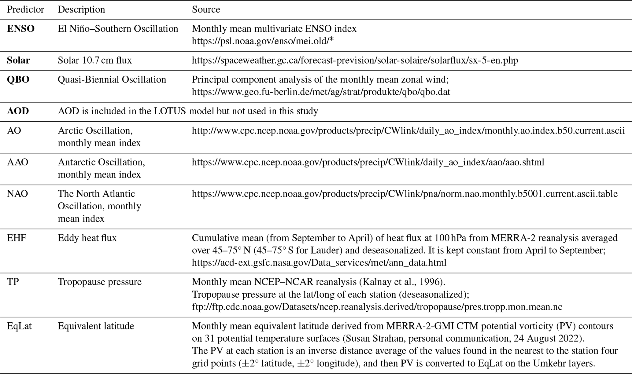
* Since the incorporation of the ENSO index into the LOTUS model, NOAA Global Systems Laboratory (GSL) has updated the index to v1.2. (https://psl.noaa.gov/enso/mei/). However, for consistency with the results from the Godin-Beekmann et al. (2022) paper, we use the old multivariate ENSO index (MEI) that is part of the LOTUS v 0.8.0 package.
Large sulfur dioxide (SO2) levels reaching the lower stratosphere following major volcanic eruptions (i.e., El Chichón, Pinatubo, or Hunga Tonga) can impact the validity of ozonesonde measured values (Yoon et al., 2022). However, SO2 is not long-lived gas and is soon converted to sulfate aerosols that can alter observations by ozone remote sensing systems. Both Umkehr and satellite ozone profiles from SBUV and OMPS are highly uncertain and/or biased because of high aerosol load during volcanic eruptions (DeLuisi et al., 1989; Petropavlovskikh et al., 2005, 2022; Bhartia et al., 1993; Torres et al., 1995; Bhartia et al., 2013). It is recommended that the data for 2 to 3 years after the El Chichón and Pinatubo large volcanic eruptions should not be used in trend analyses. Therefore, we exclude data during the volcanic periods (1982–1983 and 1991–1993) from the analyzed time series. Moreover, this study is focused on the linear trend analyses after 2000 when there are no large stratospheric aerosol perturbations that significantly influence stratospheric ozone variability over the middle latitudes and therefore impact trend and uncertainty estimates. Since we have eliminated the data during the volcanic period, this study does not include the AOD proxy in the calculations.
We define the “reference” model (RM) as the proxies most commonly used for the dynamical proxies which is equivalent to the LOTUS model v 0.8.0 minus the AOD term. The representative equation is as follows:
The QBO is derived from the Singapore radiosonde profiles (1979–2020) that detect variability in the direction of the tropical winds in the lower stratosphere. It also shows that zonal wind variation propagates downward with an average period of ∼ 28 months (Wallace, 1973). The principal component analysis of the 100–10 hPa zonal winds can describe the majority of the wind variability. The reference model (and LOTUS v 0.8.0) uses the two leading modes of the calculated empirical orthogonal functions (EOFs) for trend analyses (Wallace et al., 1993).
The El Niño–Southern Oscillation (ENSO) is a periodic mode of climate variability in the atmosphere and sea surface temperatures associated with the equatorial Pacific Ocean with periods ranging from 2–8 years. The multivariate ENSO index (MEI) is produced by the NOAA Physical Sciences Laboratory and is derived from the EOF analysis of sea surface temperature, sea level pressure, outgoing terrestrial radiation, and surface winds in the area of the Pacific basin from 30° N to 30° S and from 70° W to 100° E (Wolter and Timlin, 2011). Temperature anomalies in the troposphere with corresponding stratospheric temperature anomalies during El Niño/La Niña events modulate the tropical upwelling of the Brewer–Dobson circulation (BDC) and thus the meridional transport of ozone in the stratosphere (Diallo et al., 2018).
The solar cycle is the 11-year periodic cycle of solar activity and solar irradiance that reaches the Earth's atmosphere. The change in UV radiation that is absorbed by the atmosphere, most notably in the upper stratosphere, leads to changes in atmospheric temperature and photochemistry which produces ozone (Lee and Smith, 2003). The 10.7 cm solar radio flux data are used as the proxy for the solar cycle in the LOTUS model.
Seasonal components in the form of Fourier harmonics were added to the LOTUS model with version 0.8.0. Godin-Beekmann et al. (2022) showed in their Fig. 7 that the model fit for the ozone profile satellite and model records is improved by adding seasonal components to the proxies, increasing the adjusted R squared (R2) from 0.3 or less to 0.3 to 0.5. The seasonality and relevant contributions of some predictor variables are compensated in this study by adding the seasonal components to the fitted predictors. Seasonal components are represented in the model by sine and cosine functions with periods of 12 and 6 months that describe the variability in the proxies on these timescales. So, for each fitted predictor in the model,
a seasonal variation in the form of Fourier components is added as follows:
3.2 The extended model – adding predictors
Recent publications (i.e., Petropavlovskikh et al., 2019; Szeląg et al., 2020; Godin-Beekmann et al., 2022; Millán et al., 2024) highlight the need to reduce the trend uncertainties in the lower stratosphere (LS). There is still a discrepancy between modeled and observed ozone trends in the LS, but large uncertainties make comparisons difficult. In this study, we test additional predictors in the model to account for dynamical variability in ozone in the stratosphere, thus improving the model performance and reducing the uncertainty in the trends. The argument for additional predictors is that the LOTUS model was developed for the regression of zonally averaged ozone data, which reduces some variability that might be impacting the ground-based records on a regional basis. The impact of additional proxies in trend analyses were reported in other publications (Weber et al., 2022a; Bernet et al., 2023, and references therein) and were mostly found to improve the statistical model fit at high latitudes, where the impact of the descending branch of the Brewer–Dobson circulation and Arctic/Antarctic oscillations has contributed to additional variability in stratospheric ozone records.
In what we define as the “extended” model, we add single additional predictors (one at a time) in the model as follows:
The fitted predictors contain Fourier components, like in the reference model, to allow for seasonal variation.
We test the following additional predictors as described below to assess the impact on trends and uncertainties:
-
QBO. Two notable disruptions to the otherwise relatively periodic QBO have occurred during the study period in 2015–2016 and 2020 (Diallo et al., 2022). Two additional leading modes of the calculated empirical orthogonal functions (EOFs) are tested to improve the trend model fit during the anomalous QBO years.
-
Arctic/Antarctic oscillations (AO/AAO). The pattern of surface air pressure anomalies in the polar region and certain mid-latitude regions. The AO/AAO has strong correlations (Lawrence et al., 2020) with stratospheric ozone through the strength of the polar vortex. The positive phase of the AO or AAO in the winter months is associated with low activity in the vertically propagating planetary Rossby waves, a strong polar vortex, a low-vortex wavenumber, and low-stratospheric temperatures. Thus, the positive (negative) phase of the AO/AAO is correlated to low- (high-) ozone anomalies, especially in the winter months (Lawrence et al., 2020).
-
North Atlantic Oscillation (NAO). Similar to the Arctic Oscillation, this is a pattern of surface air pressure anomalies between certain regions in the high altitudes of the North Atlantic Ocean. This index is calculated by the pressure difference between the Azores high and the subpolar low.
-
Eddy heat flux (EHF). The flux of heat through a zonal plane by transport due to the Brewer–Dobson circulation, here averaged from 45–75° N/S (use EHF S for Lauder only). This represents the planetary wave activity that drives the transport of ozone.
-
Tropopause pressure (TP). Pressure level of the boundary between the troposphere and the stratosphere. In this study, we use the monthly mean pressure level of the tropopause from the NOAA National Centers for Environmental Prediction (NCEP) reanalysis product. As the troposphere warms due to the release of greenhouse gases (GHGs), and the stratosphere cools due to ODSs destroying stratospheric ozone, the tropopause is rising (Meng et al., 2021). Thompson et al. (2021) and Stauffer et al. (2024) found that the lower-stratospheric ozone trends in the tropics become slightly positive when recomputed with respect to the tropopause height (which has its own trend). This finding indicates that ozone depletion in the lower stratosphere (i.e., Ball et al., 2020) is driven by climate-change-related changes in transport and mixing in the lower stratosphere. Therefore, we are testing the TP proxy in the model to account for non-chemical ozone losses in order to assess the chemical attribution of ozone trends.
-
Equivalent latitude (EqLat). Geographical latitude of the isoline encircling the area of equal potential vorticity (PV) (Lary et al., 1995). The EqLat normalizes the range of PV values that change with the season and interannually and makes it convenient for the interpretation of ozone variability and trends (i.e., Wohltmann et al., 2005). The dataset was generated from Global Modeling Initiative chemistry transport model (GMI CTM) analyses (Susan Strahan, personal communication, June 2021) for each ground-based station overpass criteria (latitude and longitude envelope; see above) and at several altitude levels coincident with Umkehr ozone profile layers. Appendix C discusses a COH dataset based on EqLat instead of geometric latitude. No advantage was found using the EqLat coordinate system for the COH zonal dataset.
Source datasets for all predictors in the reference and extended models are shown in Table 3.
All proxies are used as is. No de-trending (removal of the long-term trend in a proxy) is applied to the proxies. Therefore, we interpret any changes to the trends derived with additional proxies as approximations of trends driven by chemistry and transport related to climate change. These are rough approximations as some feedbacks are known to impact chemistry (e.g., changes in stratospheric temperature).
3.3 The full model – combining additional predictors
After we have determined the impact of the additional predictors singly, we discern which predictors should be combined to constitute the “full model”. Prior to selecting additional predictors for the full model, we perform correlation tests to identify any cross-correlations between predictors. We select predictors that are not highly correlated (less than ±0.2) to ensure that all predictors are largely independent. We use the square of the Pearson correlation coefficient R2 for each pair of predictors to test our assumptions. We find that ENSO, Solar, QBO (1, 2, 3, and 4), AAO, AO, EHF (N and S), and TP (at each station) have correlations less than ±0.2 (with the exception of R2 = 0.3 for EHF (N) and AO). Therefore, any of these predictors can be combined in the full model. We find that NAO has a correlation of 0.38 with AO, so we do not use these two predictors in the same model.
We also test the independence of EqLat proxies calculated at several geographic locations (defined by the latitude and longitude of each Umkehr station) and by selecting a proxy at several altitude levels centered in the middle of Umkehr layers 3–9. We find that the R2 between the TP and EqLat in the lower stratosphere (Umkehr layer 3) can be large but anticorrelated at −0.7 (Boulder) and moderate at 0.4 (MLO and Lauder), while close to zero at Arosa/Davos and low at OHP (−0.2). In the middle and upper stratosphere, the R2 varies from −0.5 to −0.4 (MLO), 0.2 to 0.3 (Arosa/Davos and OHP), 0.5 to 0.6 (Boulder), and 0.4 to 0.7 (Lauder). EqLat has mostly low correlations (< ±0.3) with all other proxies, except for higher correlations with QBO B in layers 5 (−0.3) and 6 (−0.4) and QBO A in layer 7 (0.3) at MLO and with AO in layer 8 (0.3) at OHP and Arosa/Davos. Also, EqLat has no correlation with the TP proxy in layer 4 in Boulder, in layer 9 at Lauder, and in layers 8 and 9 at OHP. Since there are occasional high correlations between EqLat and TP proxies, we do not use them together in the “full trend model”.
4.1 Reference model trend results
First, we discuss the reference model trends derived from the COH overpass, Umkehr, and ozonesonde records at five geographic locations. All datasets are deseasonalized with a climatology computed from a subset of data taken from 1998–2008 prior to the trend analysis. Trend results are presented in Fig. 3 and organized into five panels. Each panel shows trends at selected pressure/altitude levels detected from Umkehr (green), COH (orange), and ozonesonde (blue) records at Arosa/Davos, OHP, Boulder, MLO/Hilo, and Lauder ground-based stations. Ozonesonde data for the Arosa/Davos panel are selected from Hohenpeißenberg, Germany, station that is in close proximity to Arosa/Davos station. We show trends for layers where the measurement is of the highest quality, namely Umkehr (layers 3 through 8), COH (layers 5 through 9), and ozonesonde (layers 3 through 5) records.

Figure 3The 2000–2020 ozone trends are shown at seven altitude/pressure levels. The LOTUS model v 0.8.0 is used for trend analyses. Umkehr trends (black), COH (orange), and ozonesonde (blue) are shown for five ground-based stations, namely Arosa/Davos, OHP, Boulder, MLO, and Lauder (panels from left to right). Ozonesonde data for the Arosa/Davos panel are selected from Hohenpeißenberg, Germany, which is in close proximity to Arosa/Davos. Trends from the zonal mean COH data (dashed orange line) are shown for comparison with the overpass COH data (solid line). The error bars indicate ±2 standard errors.
The Umkehr data used in this analysis are the monthly means of all available Umkehr data (one or two measurements per day). The sonde and COH monthly means use only those profiles that have corresponding Umkehr measurements on that date. We explore the impact of temporal sampling on trends in Appendix D. For COH with the Umkehr-matched data (see Fig. A12), trends are slightly larger at OHP but well within the error bars. At all other stations, the COH trends are not impacted by sampling. At OHP the ozonesonde trends matched to Umkehr (see Fig. A13) are slightly larger at layer 4 only and well within the error bars; at Lauder in layers 4 and 5 trends, are smaller but barely within the error bars.
Figure 3 shows that in the upper (above 10 hPa) stratosphere, Umkehr (black) and COH (orange) trends are positive and agree within the error bars (±2 standard errors, SEs). The exception is found at 8–2 hPa pressure level over the Lauder station, where Umkehr trends are near-zero, and COH trends are ∼ +3 % per decade to 4 % per decade. The error bars show ±2 SEs, and the fact that they do not overlap suggests that the differences in trends are statistically significant. This could be related to the relatively large uncertainties in the instrumental corrections applied to homogenize the Umkehr record (Petropavlovskikh et al., 2022). Björklund et al. (2024) discusses relative drifts in Umkehr, ozonesonde, FTIR, and MW ozone records over Lauder. The authors are not able to identify instrumental artifacts that may have caused the discrepancies in the co-located records but point out that it is not related to the sampling biases.
In the middle stratosphere (60–10 hPa), agreement between Umkehr and COH is within the uncertainty in the trend, except at Arosa/Davos, where COH trends are statistically different from Umkehr trends at 16–8 hPa. COH trends at 32–16 hPa are mostly negative (−2 % per decade to 3 % per decade), with the exception of Lauder, where trends are near-zero and similar to Umkehr trends. Umkehr trends between 32 and 16 hPa are close to zero. The ozonesonde trends (blue) agree with COH (orange) and Umkehr (black) trends in the layer of 32–16 hPa at Arosa/Davos, Boulder, and MLO. However, at OHP (Lauder) the ozonesonde trends are found to be positive at +2 ± 2.2 % per decade (negative at −3 ± 1.5 % per decade) and significantly different from the near-zero trends seen in the COH and Umkehr results.
In the lower stratosphere (125–63 hPa), Umkehr trends vary between small positive (+1 % per decade to 2 % per decade at Hilo and Lauder) and negative (−2 % per decade to 3 % per decade at Arosa/Davos, OHP, and Boulder); however, trend uncertainties are the largest (2 SEs are 2 % per decade to 3 % per decade; see Table 4 below) in comparison to the middle- and upper-stratospheric trends. Ozonesonde trends at OHP station are positive (+2 % per decade) and negative over Lauder (−2 % per decade). They also feature large uncertainties (±4.2 % per decade at OHP) that are larger than the uncertainties found in Umkehr trends which could be caused by the limited sampling (see Appendix D; Fig. D1). Sonde trends at Hilo show negative trend values with large uncertainties. But the data in this study at Hilo are not corrected for the ozonesonde drop-off after 2014 known to occur at this station (Stauffer et al., 2022), so the deviation from the Umkehr results at these levels may be misleading.
Table 4Standard error (SE) for the reference model 2000–2020 trend for five ground-based station locations (Arosa/Davos, OHP, Boulder, MLO, and Lauder). Results are provided for trend analyses of the Cohesive satellite (COH), Dobson Umkehr (UMK), and ozonesonde (SND) records. The layers are selected to represent the best quality of the data. Values of SEs shown are the actual errors in Dobson units (DU) per decade.
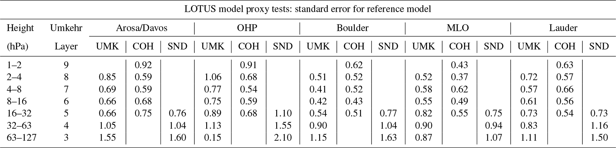
Figure 3 also shows trends derived from the zonal mean COH data associated with each station (dashed orange line). These are shown for comparison with the overpass COH data (solid line) to study the impact of the spatial sampling biases on the trends. Though Figs. 1 and 2 show clear interannual differences between the records from the individual stations and the associated zonal average, we find very small differences in trends (mostly in the upper stratosphere at middle-latitude stations). Therefore, the station overpass sampling provides trends that are representative of the zonally averaged trends (Zerefos et al., 2018), and the discrepancies in trends between GB and satellite records do not strongly depend on the spatial sampling differences.
4.2 Standard error in reference model
We will use the standard error in the linear (trend) term in Eq. (1) to evaluate the success of the additional proxies to improve understanding of trend values. The standard error is an output of the regression code and indicates the uncertainty in the trend value. Smaller standard errors indicate increased confidence in the trend result. We use the standard error as a metric instead of the standard deviation to reduce dependence on the number of points in the trend model. Table 4 provides the standard errors for the reference model fit and represents the uncertainty in the trend in Dobson units (DU) of the mean ozone in each layer at the station. The standard errors in the trend detected in three co-located ozone records at each station (or in the nearby location as in case of Arosa/Davos or MLO comparisons) do not significantly differ, although in general ozonesonde errors are slightly larger than Umkehr errors; this is most likely due to the larger sampling errors in ozonesonde monthly mean record. Also, the errors in trends detected in COH layers 5–8 are on average smaller than for Umkehr trends (with the exception of layer 7 at Boulder, MLO, and Lauder), which could be explained by an overpass method that averages several satellite profiles from adjacent orbits and therefore reduces the meteorological-scale variability in averaged ozone data.
4.3 Adjusted R2
The adjusted R2 values of the 2000–2020 trends are shown in Fig. 4 and Table 5 for the data fit using the reference model. The adjusted R2 is a modified version of R2 that adjusts for the number of predictors in a regression model and represents the goodness of the model fit to the data. For COH, adjusted R2 is shown for the overpass and the zonal datasets.
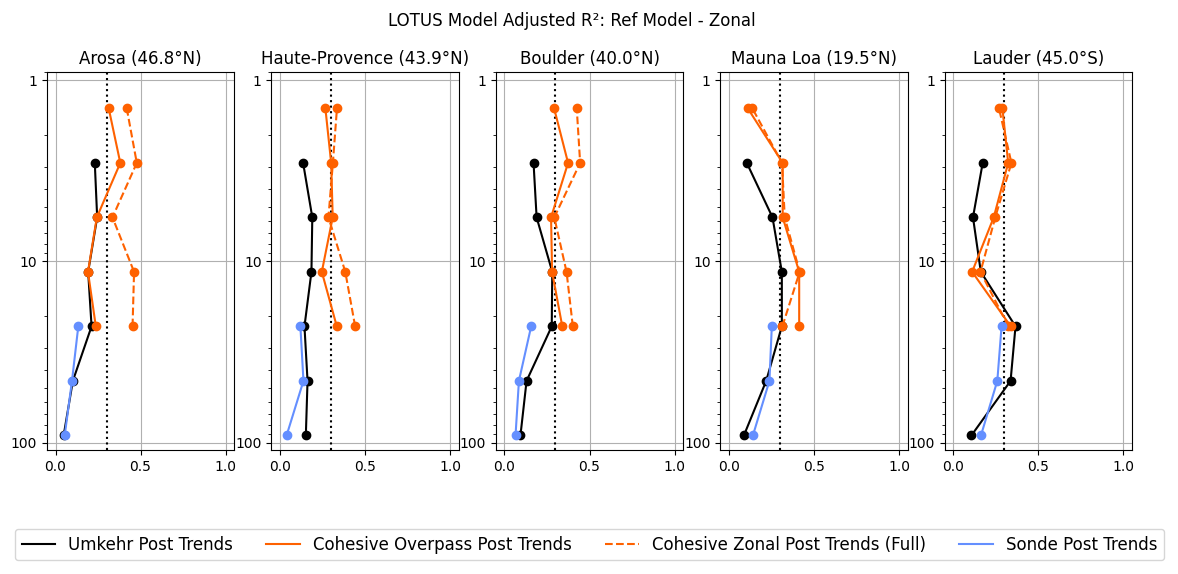
Figure 4The adjusted R2 is plotted as a function of altitude/pressure for the LOTUS model fit to Umkehr (black), ozonesonde (blue), COH overpass (solid orange), and COH zonal mean (dashed orange). Results are shown in five panels that represent trend analyses of ozone records over Arosa/Davos (Hohenpeißenberg for sondes), OHP, Boulder, MLO (Hilo for sondes), and Lauder ground-based stations.
Table 5Similar to Table 4 but for the adjusted R2. Values of 0.30 and above are indicated in bold as a threshold to indicate a satisfactory fit.
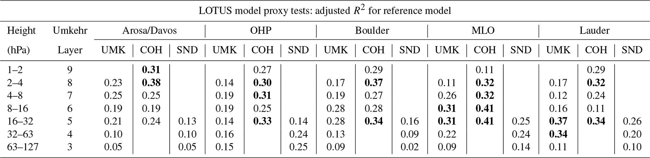
Though values are significantly less than the high values usually seen when comparing data that include the prevalent seasonal variation, the adjusted R2 values for the COH zonal mean record are similar in magnitude and vertical shape compared to the results of the (60° N–60° S) broadband trend analyses published in Godin-Beekmann et al. (2022), with Fig. 7 varying between 0.1 and 0.5. We designate the average values (0.3) as a threshold for satisfactory fit, indicating conformance with prior LOTUS results. We indicate, in bold in Table 5, the adjusted R2 values of 0.3 or greater to note the achievement of that threshold and include a dashed vertical line in Fig. 4 for reference.
The adjusted R2 for the reference model fit is slightly better for the zonal mean COH data than for the COH overpass over the northern middle-latitude stations. This is expected as much of the variability in the time series is reduced in the zonal average compared to the station overpass data, as shown in Fig. 2, and more easily explained by the typically used predictors. Indeed, the goal of this study is to determine if the additional predictors help to explain the additional variation as measured at point locations.
The model fit to the GB data is similar to the COH overpass results in the middle stratosphere (layers 5 and 6), but the model explains less of the ozone variability in the Umkehr records in the upper stratosphere (layers 7 and 8). In the lower stratosphere (layers 3, 4, and 5), the model fit to the ozonesonde and Umkehr records is similar, with the exception of Lauder (Umkehr has larger adjusted R2 in layers 4 and 5). The adjusted R2 for COH overpass in layer 5 is similar to Umkehr and sonde, with a larger difference at OHP. The adjusted R2 in the lower stratosphere is less than in the middle stratosphere, which points to other processes (e.g., transport) that drive ozone variability. In this paper, we investigate improvement to the trend model fit by introducing additional proxies that can improve the representation of the dynamically driven ozone variability in the stratosphere.
4.4 Reference model p values
The p values are often used to evaluate the statistical significance of predicted results and results labeled “significant” if they remain below a threshold of 0.05. However, Chang et al. (2021) argued, as Wasserstein et al. (2019) do, that all trends should be reported with their associated p values and a thorough discussion of the certainty in trend detection as described by the p values. Therefore, the p values can be used for understanding the certainty in the trend. Under the International Global Atmospheric Chemistry Project's Tropospheric Ozone Assessment Report (IGAC TOAR) activity, p values are scored to define a consistent scale for comparison of the trends between different analyses (see Table 3; Chang et al., 2023).
Table 6 provides p values for the reference model. These are further used as a baseline for comparison to model fits with additional predictors. p values of the reference model fit suggest a high certainty (p < 0.05) in the detected trends in the COH data in layers 7, 8, and 9 at almost all stations with the exception of the higher p value (0.1; medium certainty) found at MLO in layer 9. Also, high certainty in derived trends is reached for COH records in layer 5 at Boulder and MLO.
Table 6Similar to Table 4 but for p values. Values of less than 0.05 (high certainty in trend detection) are shown in blue and with bolded numbers. Values between 0.05 and 0.1 (blue not bolded) indicate medium certainty. Between 0.1 and 0.33 (orange) there is a low certainty in trend detection. Above 0.33 (red), there is a very low certainty or no evidence of trend detection.

Umkehr trend analyses also show high confidence in the trend detection at Arosa/Davos and MLO stations in layers 6, 7, and 8; at OHP in layers 7, 6, and 8; and in Boulder in layers 6 and 8. For the ozonesonde data, high confidence (i.e., low uncertainty) is found for Hohenpeißenberg and Boulder trends detected in layer 5 and at Lauder in layers 4 and 5.
The medium level of the certainty (0.05 < p ≤ 0.10) is found in trends detected in layer 5 of the COH ozone time series at Arosa/Davos, layer 3 of ozonesonde at MLO, and in layer 4 of ozonesonde and layer 3 of Umkehr at Lauder.
Low certainty in detected trends at a p value of 0.10 (not inclusive) to 0.33 is found in Umkehr layers 3 and 5 at Arosa/Davos, in COH layer 5 and Umkehr layer 3 at OHP, in Umkehr layers 3 and 4 and ozonesonde layers at Boulder, and in ozonesonde layer 4 and COH layer 6 records at MLO.
The highest (lowest-certainty) p values (> 0.33) were found in layer 6 of the COH overpass records at most stations (except for MLO, where p values are medium-high). We note that the COH trends are close to zero, and the uncertainty envelope crosses the zero line. Therefore, the statistical trend model cannot separate trends from zero due to unexplained high-ozone variability in this layer. Similarly, near-zero Umkehr trends with relatively large SEs in layer 6 at OHP and Lauder, layer 5 at all (except Arosa/Davos) stations, and layers 3 and 4 at MLO show the same level of high p values, thus suggesting that additional proxies should be added in the trend model to assess the impacts of the natural variability and instrumental noise on trend uncertainty.
It is also important to note that the reference trend model fit to ozone in Umkehr layers 7 and 8 at Lauder has high p values, which is related to the near-zero trends that show large disagreement with the COH trend. This difference could be caused by remaining instrumental step changes that were not fully removed during the record homogenization (Petropavlovskikh et al., 2022).
While near-zero trends and high p values are found in the fit of the Hilo ozonesonde record in layer 5, the p values in layer 4 show only medium p values for near-zero trends. It is possible that infrequent launches of ozonesonde observations at Hilo could create a temporal sampling bias and appear noisy. The ozonesonde record at Hohenpeißenberg has sufficiently frequent sampling (3 times per week) for successful trend analyses (Chang et al., 2020; Chang et al., 2024), but the p values remain high in layers 3–4. The p values for Umkehr fit at Arosa/Davos are in the medium to high range for layers 3, 4, and 5 but somewhat smaller, which could be due to non-zero trends in layers 3 and 5. The p-value difference could be also related to the different locations of the ozonesonde (HOH) and Umkehr (Arosa/Davos) observations; thus, the records could contain different atmospheric variability that might impact the model fit.
We will discuss changes to the p values in the next section after we add more proxies to the trend model in an attempt to improve confidence in trend detection.
The LOTUS-styled reference model is developed and optimized for zonal average datasets. Modeling and trend analysis for GB and satellite overpass data may be improved by the addition of other proxies not used in the reference model to improve capturing processes that impact ozone changes over limited geographical regions. The extended model tests the addition of single predictors to see if fit statistics can be improved for GB and overpass datasets. We judge the success of the extended model by examination of the reduction in the standard error in the trend term and by evaluation of the impact on the adjusted R2 of the model fit. Table 7 displays the change in the standard error in the post-2000 trend for each proxy tested and determined as SEref−SEext as a percent of SEref. As such, positive values correspond to the desired reduction in SEs and are highlighted in the table in blue. Low-impact changes in the SEs are highlighted in white, and increases in the SEs (negative values) are highlighted in red. It may seem unusual for the addition of proxies to increase the SEs (negative values in the table); this indicates less confidence in the fit. But these SEs are the uncertainty in the trend term and not in the overall model fit. The new proxies considered each have a possible trend and associated error budget for that trend. Whether the additional proxy increases the trend uncertainty can depend on how well the trend of the new proxy can be characterized. The adjusted R2 is a better indicator of the overall model improvement. Figure 5 displays the adjusted R2 for the extended model for each proxy tested. Values of 0.30 and above are indicated in bold as a threshold to indicate a satisfactory fit.
Table 7Change in the standard error (SE) of the post-2000 trend estimate, in percent of SEs of the reference model for adding single predictors. (a) Tropopause pressure; (b) equivalent latitude; (c) QBO terms C and D; (d) AO/AAO; (e) NAO; (f) eddy heat flux. Cells with reduced (increased) SEs have a blue (red) background, while cells with low-impact changes (< 0.5 %) have no colors.
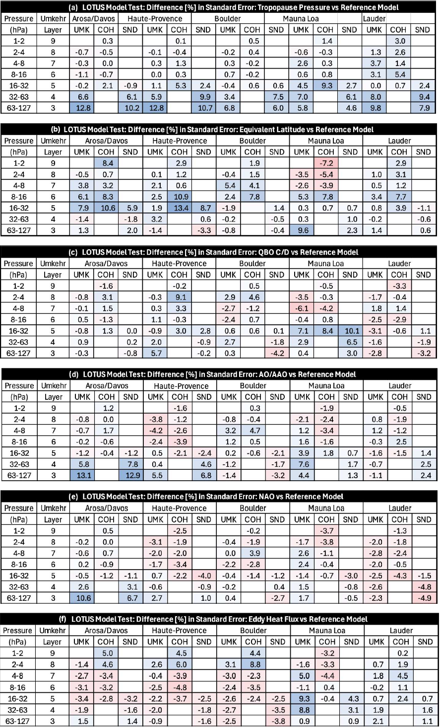
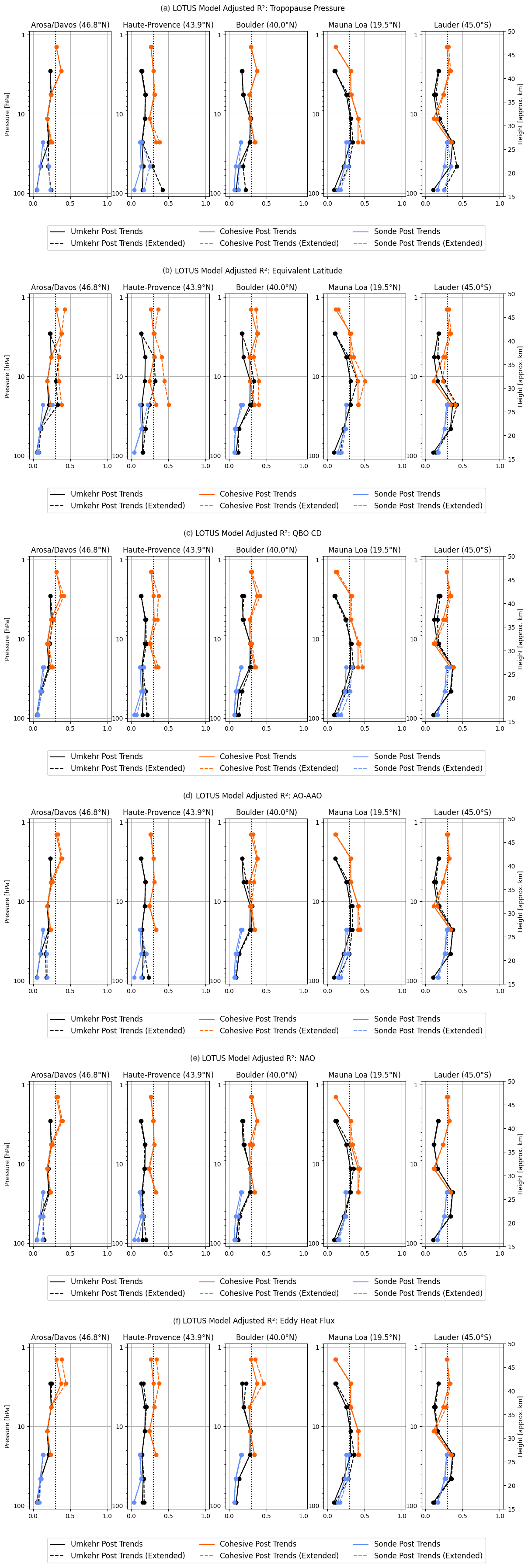
Figure 5(a) Similar to Fig. 4 but adjusted R2 results are shown for both the reference model (solid line) and the extended model (dashed line; full) for COH overpass (orange), Umkehr (black), and ozonesonde (blue) trends. The extended model includes additional TP proxy. (b) The same as panel (a), but the extended model includes an equivalent latitude proxy. (c) The same as panel (a), but the extended model includes two extra QBO terms as an additional proxy. (d) The same as panel (a), but the extended model includes the AO/AAO proxy. (e) The same as panel (a). but the extended model includes NAO as an additional proxy. (f) The same as panel (a), but the extended model includes EHF as an additional proxy.
5.1 Tropopause pressure (TP)
Adding the TP proxy to the standard LOTUS model produces the most consistent results between different techniques (COH, Umkehr, and ozonesonde) and also has a similar magnitude of the standard error changes among different latitudes (i.e., Arosa/Davos, OHP, Boulder, MLO, and Lauder). The most significant impact in improving the SEs is found in the lower stratosphere (layers 3 and 4) and in the middle stratosphere (layer 5) at the MLO tropical station. The impact of the TP proxy on the COH trend uncertainty in the model stratosphere (layer 5) is somewhat larger, likely due to the satellite AK extending into the lower stratosphere. Similarly, a larger reduction in the standard errors in the Umkehr trends in the lowermost stratosphere (layer 3) in comparison to the AK-smoothed ozonesonde record could be due to sampling biases in the ozonesonde record. Adding the TP proxy to the reference model improves the adjusted R2 in layers 3–5, whereas the SE improvements are also consistent across geolocations and measurement techniques. The TP proxy only explains ozone variability near the tropopause because changes in both parameters are linked to the same dynamical processes (i.e., irreversible mixing). In the middle and upper stratosphere, ozone variability is not linked to the processes that change TP; thus, using this proxy adds an error to the model fit. Several improvements resulted in adjusted R2 to exceed the 0.3 threshold (Umkehr at OHP in layer 3 sonde and Umkehr at Lauder and MLO in layer 4); in many cases, the adjusted R2 increased by more than 0.02 (see Fig. 5a).
5.2 Equivalent latitude (EqLat)
In the mid-latitudes, the addition of EqLat as a predictor shows consistent results across measurement techniques and stations with few exceptions. The reduction in the SEs of the model fit is evident in the COH data in the upper stratosphere (above 4 hPa or ∼ 40 km) but is less pronounced in Umkehr profiles. The impact on MLO SEs of the trend fit in the upper stratosphere is negative (in both COH and Umkehr records), which can be explained by the fact that the EqLat is much closer to geometric latitude near the Equator than at the middle/high latitudes, and therefore its use as a proxy would not provide any additional information in interpretation of the tropical upper-stratospheric ozone variability. It could also suggest that the addition of EqLat will overfit the record.
The ozone record trend fits in the middle stratosphere (32–4 hPa or 25–40 km) benefit from adding the EqLat proxy at most locations. Improvement in the SEs of the trends in the lower stratosphere (127–63 hPa or ∼ 15–20 km) is minimal and limited to some locations and instrumental records (Arosa/Davos Umkehr and HOH sonde, MLO Umkehr and sonde, and Lauder Umkehr and ozonesonde), which could be related to the location of subtropical jet that modulates mixing of tropical and subtropical (and occasionally polar) air masses and influences the stratosphere–troposphere exchange. Unexpectedly, the addition of the EqLat proxy to the MLR statistical model for trend detection in Boulder Umkehr and ozonesonde lower-stratospheric ozone records increases the uncertainties in the fit, while the influence of subtropical jet on Boulder lower stratosphere is well known (Manney and Hegglin, 2018). Perhaps the data analyses also need to consider the tropopause variability?
In terms of the impact on the adjusted R2, the EqLat proxy significantly improves the model fit for multiple instruments, mostly in layers 5–7 and in COH fit in layer 9 (see Fig. 5b). The adjusted R2 improvements also often exceeded the 0.3 threshold. No significant improvement is found in the ozonesonde model fit in layer 5, with the exception of the OHP and Hohenpeißenberg records (0.1 increase).
5.3 Extra QBO terms C and D
QBO is an important driver of ozone variability at tropical stations. Based on the results of adding two extra terms of the QBO to the standard model, the recommendation could be to exercise this option only for the tropical station trends. At the northern middle latitudes (i.e., in Arosa/Davos, OHP, and, to a lesser degree, Boulder) an improvement in the trend SE uncertainties in layer 8 is noted. There seems to be a similar pattern for the upper stratosphere in trends derived with a heat flux. Tweedy et al. (2017) show that the first two EOFs of the QBO did not describe the anomalous QBO behavior, while Anstey et al. (2021) show that the addition of two more EOFs of the QBO could capture the effect of the disruptions on the zonal winds. Therefore, including additional QBO empirical orthogonal functions (EOFs) could benefit the attribution of ozone variability in the middle stratosphere (layers 4 and 5) in the tropical latitudes (reduced errors in MLO/Hilo trends) and in the upper stratosphere (layer 8 in COH and in some Umkehr trends) in the NH middle-latitude stations (Arosa/Davos, OHP, Boulder) related to the global circulation pattern that is also represented by the heat flux proxy. A slight reduction in the errors at SH middle latitude (sonde at Lauder, Aotearoa / New Zealand) could be invoked by the EqLat variability that has a small correlation with the QBO D proxy and sampling bias. A reduction in SEs in the trend fit of the layer 5 ozonesonde (up to 2.8 %) and COH (up to 3.0 %) records at OHP is not found in the Umkehr results, which suggests overfitting and sampling bias (see the results in Appendix D).
The addition of extra QBO terms slightly improves the adjusted R2 model fit (see Fig. 5c) for all COH station overpass records in layer 8 (except at MLO) and occasionally improves the Umkehr adjusted R2 (Boulder and Lauder). The most significant improvement is found at MLO in layers 3–5 in all three instrument records.
5.4 Arctic and Antarctic oscillations (AO/AAO)
AO/AAO proxies reduce SEs (blue-colored cells) in the lower stratosphere (layers 3 and 4) at Arosa/Davos, OHP, and MLO, although the reduction somewhat differs between the Umkehr and ozonesonde records. At the same time, at Boulder and Lauder, the SE does not show an improvement after the addition of the AO/AAO proxy (AAO is used instead of AO at Lauder). In the middle stratosphere (layer 7), a reduction in SEs is found over Boulder in COH and Umkehr records. The addition of AO/AAO proxies improves the SEs of the trend at MLO and Lauder but only in Umkehr records, while it worsens the COH SEs. At Lauder, the COH SEs in layer 6 show an improvement but not in the Umkehr record. Since results in the middle stratosphere (layers 5–7) are not always consistent among different techniques (reductions are not in the same layers), it could indicate a statistical model overfit into the record's noise or vertical smoothing of the Umkehr or COH technique that combines ozone variability in the layer with a portion of ozone variability in the adjacent layers, thus partially or completely reducing the correlation with the proxy.
The addition of the AO predictor increases the adjusted R2 in the lower stratosphere at Arosa/Davos, OHP, and MLO (see Fig. 5d). Also, a small enhancement of the adjusted R2 is seen in the middle and upper stratosphere, including in Umkehr layers 6 and 7 and COH layers 6, 7, and 9 over Boulder, as well as in the Umkehr fit in layers 5–7 at MLO and at Lauder (AAO) for Umkehr and COH records in layer 6. These results are not very consistent across different geolocations but seem to be consistent across instrumental records at some stations (Umkehr and ozonesonde in the lower layers and COH and Umkehr in the upper layers).
5.5 North Atlantic Oscillation (NAO)
Including the NAO proxy in the trend model appears to have a similar pattern (i.e., in latitude and altitude) of changes in the standard error compared to the result of the inclusion of the AO/AAO proxy. It is not a surprise, since indices of the NAO and AO are highly correlated in time due to their common link to the downward propagation of stratospheric anomalies. Standard errors are somewhat reduced in the lower-stratospheric layers at the middle-NH latitude and tropical Umkehr records, but the change is less significant than in AO/AAO cases. The impacts on ozonesonde trend uncertainties are very minimal and inconclusive at Boulder (layers 5 and 4), Hohenpeißenberg (layers 3 and 4), and OHP (layer 3). The impacts on Lauder are similar or stronger (SEs are increased for Umkehr and sonde records) to the impacts of the AO/AAO. In the middle and upper stratosphere, the standard errors are typically increased. The exception is found in layer 7 of the COH record at Boulder and Arosa/Davos and in layers 6 and 7 of the Umkehr record at MLO. Similar negative results are found when AO/AAO proxies are added, which suggests that the observed time series are overfitted and potentially some instrumental or sampling anomalies are misinterpreted with the addition of these proxies (see Fig. 5e).
5.6 Eddy heat flux (EHF)
The EHF represents a dynamical proxy for an assessment of the impact of the Brewer–Dobson circulation (BDC). It is expected to have an impact on the upper-stratospheric ozone by accelerating the transport in the upper branch that brings more ozone at higher latitudes (i.e., Arosa/Davos) and middle latitudes (i.e., OHP, Boulder, and Lauder). It could possibly represent changes in the lower branch of the BDC circulation and the expansion of the tropical band, thus modulating ozone in the lower stratosphere at tropics (i.e., MLO). In the southern middle latitudes (i.e., Lauder), the correlations could be related to the shift in the subtropical wave activities to the higher latitudes in response to the ozone hole healing.
The addition of the EHF predictor leads to reduced SE uncertainties in the upper stratosphere in COH and Umkehr trends at OHP and Boulder and in COH-only trends at Arosa/Davos. It has a much smaller reduction in SEs for the Lauder trend and even an increase in uncertainties if used to fit the upper-stratospheric ozone time series at MLO. At the same time, the SEs in the Umkehr and ozonesonde middle stratosphere (layers 4–5) at MLO are substantially reduced, including smaller improvements at Lauder. In the lower-stratospheric (layer 3) ozone trend, SEs in Umkehr and sonde records at MLO, Lauder, and Arosa/Davos are somewhat reduced when using the EHF proxy.
The addition of the EHF predictor seems to have an impact in the upper stratosphere increasing the adjusted R2 for COH records in layers 8 and 9 in all except the MLO or Lauder records, which indicates the impact of the BDC upper branch on the middle-NH latitudes (see Fig. 5f). In contrast to the COH, the Umkehr adjusted R2 has not changed significantly, which possibly suggests a high measurement noise in the station records. There is, however, a small increase in adjusted R2 in the Umkehr record in layer 7 at MLO (whereas COH does not show a change).
The increase in adjusted R2 is found at MLO in Umkehr and sonde layers 4 and 5, including a small increase in layer 3, which probably is related to the EHF-driven changes in the middle stratosphere. Ozone variability in Umkehr and sonde records at MLO appears to contain information about the circulation changes in the shallow BDC branch.
In this paper, we seek to develop an improved model and thus trend estimates for point-located measurements of ozone through modifications of a model optimized for zonal data. Our criteria for model improvement are based on the reduction in the SEs of the trend with either improvement (at best) or moderate impact (at worst) on the model's adjusted R2. From the results of the previous section, we see several opportunities to improve the model and improve confidence in the trend estimates. This section examines if the gains of the above are improved while adding several predictors together. As stated above, the TP as a predictor exhibits the most consistent results for all stations and measurement techniques. The other predictors have successes in the SE reduction but only at some layers and some stations. Some results are instrument-dependent.
Based on the tests above, we expect that combining predictors can improve the model fit and trend SE reduction, but it is clear that the predictor selection should vary by station and level. Appendix E details the choices made for the full model which combines 1 to 3 additional proxies beyond the reference model.
6.1 Predictors added for the full model
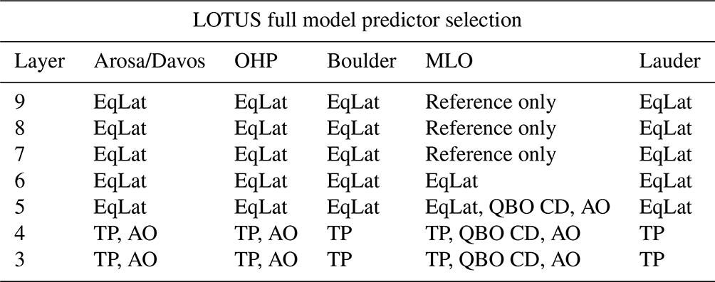
Reduction in the SEs of the trend while improving (or at least not impacting) the model's adjusted R2 is the basis of predictor choice for the full model. To qualify, a predictor should exhibit consistent results for all measurement techniques. Improvements at multiple stations is preferred to single-station improvements. In general, we avoid combining highly correlated predictors. Table 8 shows the final choices for the full model.
Table 8Added predictors for the full model are tuned for each layer and each station. For layers 7 to 9, the SEs and adjusted R2 parameters at MLO are not improved by additional predictors, and the original LOTUS-based reference model is used. Appendix E explains the logic of the predictor selection.
6.2 Impact of the full model on trends
Figure 6a shows the trends for the stations (with COH overpass) for the reference and full models. The impact of the full model on ozone trends derived in the upper stratosphere (above 16 hPa) is neutral. The addition of proxies to the LOTUS model does not change trends that remain the same magnitude as those derived using the reference model, i.e., positive and statistically significant at the SH and MH middle latitudes and over the tropics. The largest difference (outside of the SE uncertainty) between upper-stratospheric Umkehr and COH trends is found over Boulder, MLO, and Lauder.
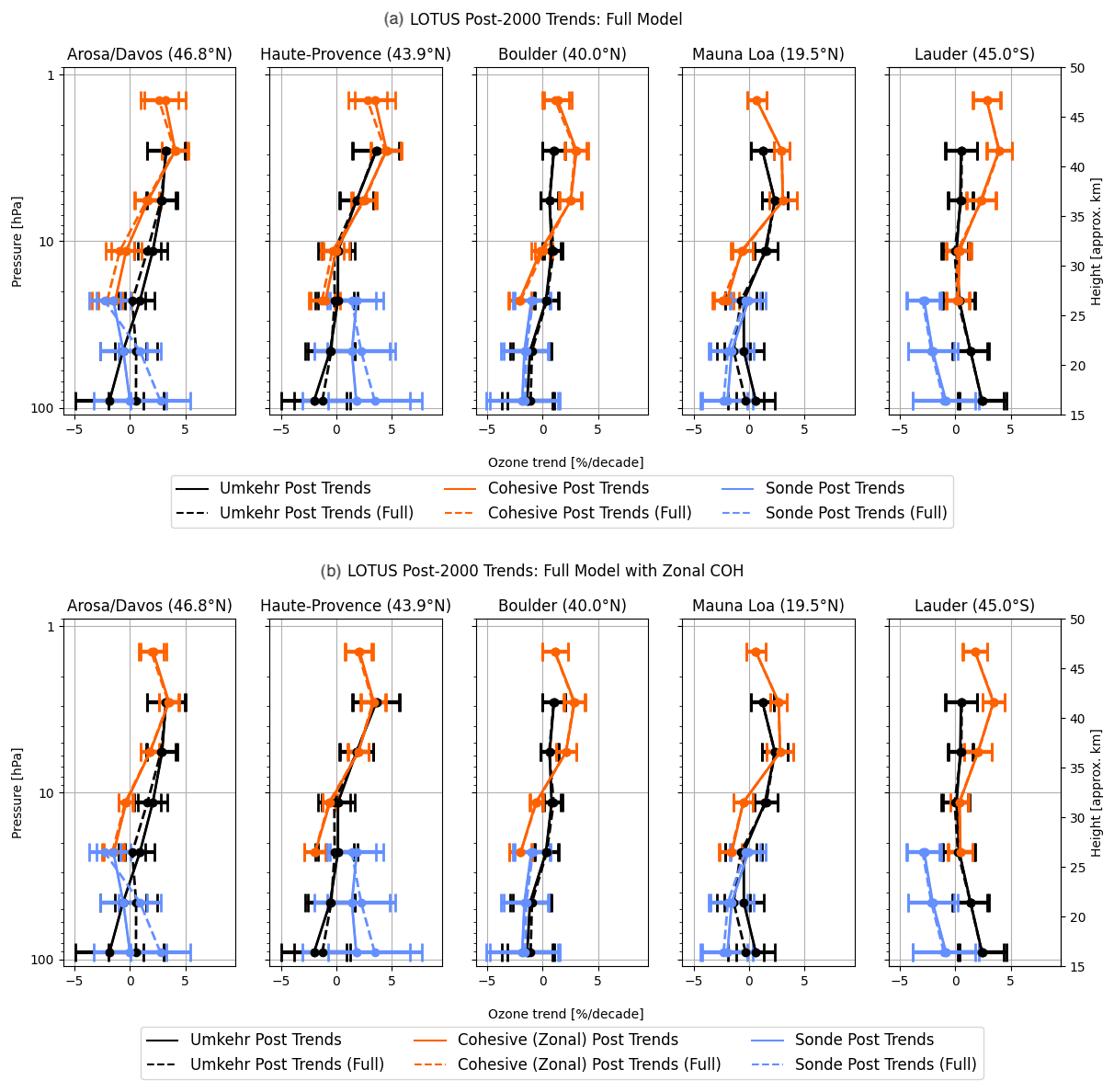
Figure 6(a) Post-2000 trends for the full and reference models. In this figure, the COH data shown in orange are the overpass data. Solid lines depict reference model values (unchanged from Fig. 3). Dashed lines depict full model values for all three instrument types. (b) Post-2000 trends for the full and reference models. In this case, the orange lines are with the zonal data instead of the COH overpass data. Dashed lines depict full model values for all three instrument types. The Umkehr and sonde trends are unchanged from panel (a).
In the middle stratosphere, additional proxies do not change trend values across locations and instrumental records (outside of the SEs). At OHP, Boulder, and Lauder, Umkehr trends in layer 6 (8–16 hPa) are barely positive, while COH trends are negative. At Arosa/Davos and MLO, COH trends in layer 6 are barely negative, and Umkehr trends are significantly positive. Most COH trends in layer 5 (16–32 hPa) are statistically negative (except at Lauder), while Umkehr trends are near-zero.
In the lower stratosphere, Umkehr and sonde trends at Arosa/Davos and MLO change after the full model is used. However, Umkehr and sonde trend changes at MLO are within the SEs and therefore can be deemed not significant. Ozonesonde trends at Arosa/Davos in layer 3 (125–63 hPa) change from zero to positive. Umkehr trends at Arosa/Davos in layer 3 change from negative to near-zero. Large differences between ozonesonde and Umkehr trends at Lauder and OHP remain unchanged after the full model is applied, although the respective SE envelopes overlap.
Figure 6b also shows the trends for the reference and full models, but the COH data shown are the associated zonal data relevant to each station. The incorporation of the additional proxies does not change the trend values for the zonal COH data. The impact on error estimates for the trends is discussed next.
6.3 Impact of the full model on the trend SEs
Table 9 summarizes the reduction in the SEs for the full model. The selection of the EqLat predictor for the full model in layers 5–9 and for all stations (except MLO/Hilo; to be discussed later) shows the improvement in the SEs (as discussed in the previous section). Also, the TP predictor is selected for inclusion in the full model for trend analyses at Boulder and Lauder stations in layers 3 and 4. The combination of several predictors is used for individual stations based on the additional reduction in the SEs. For the Arosa/Davos and OHP stations, we select a combination of the TP and AO to reduce the SEs by almost twice as much in some layers. The inclusion of the AO proxy is in support of the interpretation of seasonal and interannual ozone variability recorded over stations in Europe that are north of 40° latitude and are exposed to the seasonal events of ozone-depleted air masses transported from the polar region during the spring season (Steinbrecht et al., 2011; Manney et al., 2011; Knudsen and Grooss, 2000; Fioletov and Shepherd, 2005; Zhang et al., 2017; Weber et al., 2022a). The strong impact of AO/AAO on the lower-stratosphere ozone variability is not detected in Boulder or Lauder, and we choose not to include it in the full model for trend analyses at these stations.
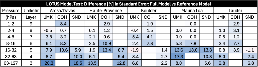
Table 9Change in post-2000 trend SEs in the full model as a percent difference in the reference model. Color-coding is the same as that introduced in Table 7.
The MLO/Hilo location is close to the tropical belt and therefore has different processes impacting stratospheric ozone variability, as discussed in the previous section. We find that EqLat proxy can be added to the full model in layers 6 and 5 (similar to other stations); however, above layer 6, EqLat or TP is not useful for the interpretation of tropical ozone variability, and therefore, we believe the trend model in these layers should remain as it currently is used in Godin-Beekmann et al. (2022) analyses. The EqLat and TP are mildly correlated (−0.4) in the stratosphere, and therefore we decided against combining both of these proxies in the full model. However, we also found that adding AO and QBO C/D proxies in layers 3, 4, and 5 improved the model fit and reduced the SEs. These combined additional proxies are not correlated and reduce SEs more than when using them separately.
The full model showed impacts on the SEs in the upper stratosphere (above 8 hPa). The trend errors were reduced, with the exception of Umkehr trends at 4–2 hPa over Boulder and Arosa/Davos, where errors did not change. No changes in SEs are found at MLO with additional proxies; thus, the full model is kept the same as the reference model for this station in the upper stratosphere.
Similarly, in the middle stratosphere, SEs were mostly reduced after the full model was applied (except for slightly larger SEs in trends derived from ozonesonde at OHP and from Umkehr at Boulder).
After applying the full model in the lower stratosphere, we still found high uncertainty due to higher-ozone variability (natural variability), but SEs were reduced. Arosa/Davos and MLO Umkehr and sonde trends changed after full model was used. The change in ozonesonde trends at Hohenpeißenberg in layer 3 (125–63 hPa) goes from zero to positive, and trend detection becomes highly confident (p value < 0.05). Umkehr trends at Arosa/Davos in layer 3 changed from negative to near-zero, but results have low certainty (p value > 0.1). Larger trend differences remain between ozonesonde and Umkehr at Lauder and OHP after the full model is applied.
It is instructive to ponder if the addition of proxies that yield improvements via a reduction in the standard error in the localized GB or overpass measurements also has the potential to improve uncertainties in the zonal data. To explore this, Table 10 and Fig. 7 show the percent change in SEs of the trend when adding the proxies for the full model. Values are shown for both the COH overpass and the COH zonal data. In general, except when the improvement in the SEs for the overpass COH is small (3 % or less), the addition of proxies has much less impact on the zonal results than on overpass results. This suggests that indeed the reference LOTUS model is well tuned for zonal datasets but can be improved with the select addition of proxies for overpass or localized GB data.
Table 10Change in the standard error in the trend as a percent of the reference model SEs for the COH overpass data and zonal data at the five ground stations. The MLO full model in layers 9–7 is the same as the reference model (therefore, it is marked as not applicable (NA)).
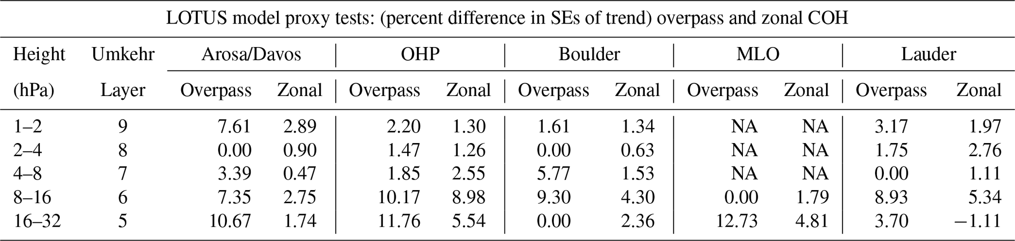
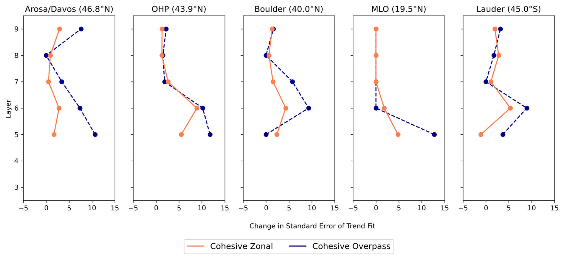
Figure 7Change in the standard error in the trend as a percent of reference model SEs for the COH overpass data (blue) and COH zonal data (red) at the five ground stations.
6.4 Impact of the full model on adjusted R2
Table 11 shows the adjusted R2 for the full model. In the upper stratosphere, the full model increases the adjusted R2 above 8 hPa (except in Umkehr at 4–2 hPa). Over MLO, there is no change because the full model is kept the same as the reference model for layers 7, 8, and 9.
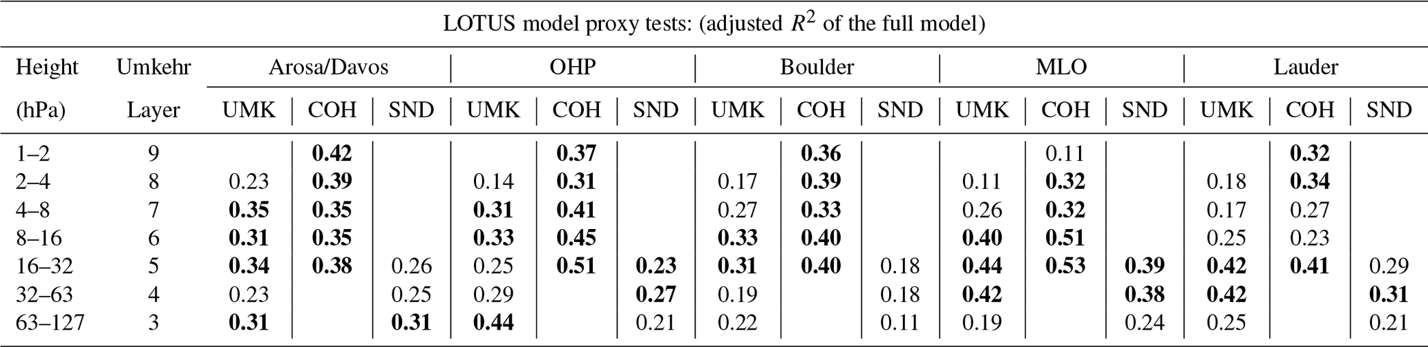
Table 11Adjusted R2 of the full model. Values of 0.30 and above are indicated in bold as a threshold to indicate a satisfactory fit. Compare to Table 4, which contains values for the reference model.
In the middle stratosphere (32–8 hPa), adjusted R2 increases are found in all records (although smaller increases are found in ozonesonde and Umkehr records at OHP, Boulder, and Lauder at 32–64 hPa). At Arosa/Davos, Boulder, and Lauder, the adjusted R2 in the COH and Umkehr trend models increase and continue to be very close in value. The COH adjusted R2 is larger at OHP and MLO than in Umkehr and sonde records, suggesting that overpass conditions might have smoothed some natural variability observed in the GB records. In general, the adjusted R2 is the largest at the 32–64 hPa level. This suggests that the full model shows an improvement for regional trend analyses in the middle stratosphere.
Although Umkehr and sonde trend changes at MLO in the lower stratosphere are within the SEs and therefore can be deemed not significant, the adjusted R2 is increased, which suggests a better model fit in the full model. The adjusted R2 increases in both Umkehr and ozonesonde data, while the largest increases are found in the Arosa/Davos, OHP, and MLO records.
In the lower stratosphere, the adjusted R2 remains low in both Umkehr and sonde records at Boulder (only TP is added for the full model). While the p values at 63–32 hPa are significantly reduced (see the discussion in Sect. 6.5), they still remain relatively high. These results suggest that additional research is needed to identify the best set of proxies for Boulder records in the lower stratosphere. At Lauder, the ozonesonde record shows a smaller adjusted R2 compared to Umkehr, partially due to low sampling biases.
It is valuable to further explore the impact of the full model on the adjusted R2 for the zonal and overpass COH data. Figure 8a shows the adjusted R2 for the reference and full models at each of the five stations using the COH overpass data. In all cases, the full model improves the adjusted R2 except for MLO layers 7, 8, and 9, where the full and reference models are identical. The most significant improvements are seen by Umkehr at layers 3 to 7; the COH overpass at layers 5, 6, and 7; and sonde layers 3–5. Figure 8b shows similar results using COH zonal data instead of the overpass. There is practically no further improvement in the adjusted R2 for the zonally averaged COH results (except for a small increase for MLO layer 5). A comparison of the results reveals that for OHP the implementation of the full model for the COH overpass data (Fig. 8a; dashed line) improves the adjusted R2 to values nearing that of the reference model zonal data in layer 7 and below (Fig. 8b; solid line). For MLO and Lauder, the use of the full model on the COH overpass data improves the adjusted R2 over the reference model beyond the improvement seen in the COH zonal results for layers 5 and 6. At Arosa/Davos and Boulder, the implementation of the full model does not fully reach the magnitude of the COH zonal adjusted R2.
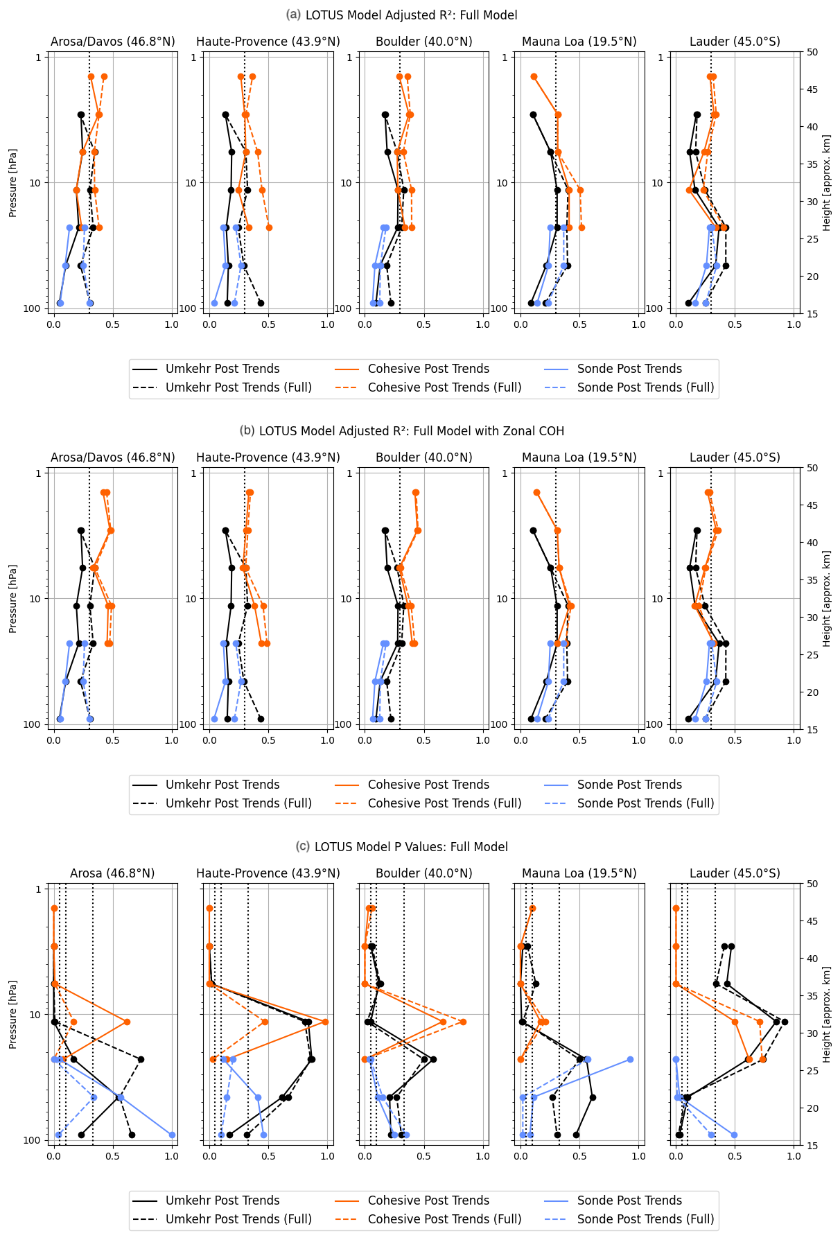
Figure 8(a) Adjusted R2 for the full model (dashed lines) and reference model (solid lines) at five stations. The COH data in this figure are the overpass data at each station. (b) Adjusted R2 for the full model (dashed lines) and reference model (solid lines) at five stations. The COH data in this figure are the zonal data for each station. The Umkehr and sonde lines are identical to those in panel (a); (c) the same as panel (b) but for the p values. Vertical dotted lines indicate limits for the high (< 0.05), medium–high (between 0.05 and 0.1), medium (between 0.1 and 0.3), and low confidence (> 0.3).
6.5 Examination of the p values of the full model
In the upper stratosphere (above 8 hPa), the confidence in Umkehr trends remained high (see Fig. 8c) for most stations, except at Boulder (medium to low) and Lauder (very low, although some improvement was found). COH trend confidence was very slightly degraded over Boulder at 1–2 hPa but mostly has not changed.
In the middle stratosphere (between 32 and 8 hPa), p values were significantly reduced in COH records. At 8–16 hPa, values remained high, but at 16–32 hPa the confidence improved (continued) to high over Arosa/Davos and OHP (Boulder and MLO). In the case of Umkehr analyses in layer 8–16 hPa at Arosa/Davos, Boulder, and MLO, the confidence remained high. However, at 16–32 hPa the Umkehr trend detection confidence was degraded over Arosa/Davos and Lauder. For the ozonesonde record, the p values remained low (< 0.05), except at MLO, where some improvement was found after the full model was used, but the p value remained high. It suggests that some instrumental records have either high-atmospheric or instrumental noise, and therefore, perhaps a high certainty in the trend detection cannot be achieved with linear trend models. For near-zero trends with high variability, the p values are not a good criterion for trend detectability.
In the lower stratosphere (between 125 and 32 hPa), analyses of p values for the full model fit show significant improvement for Umkehr trends at MLO between 63–32 hPa (while the p value was increased at other stations at this level). In addition, the improvement in p values was found for ozonesonde trends at all stations. Specifically, very low p values for the full model were reached at Arosa/Davos (125–63 hPa), OHP (125–63 and 63–32 hPa), MLO (125–63 and 63–32 hPa), and Lauder (63–31 hPa).
We find that upper-stratospheric trends in COH overpass and Umkehr records detect ozone recovery with high confidence (p < 0.05) above 8 hPa (with the exception of near-zero positive Umkehr trends over Lauder and Boulder). We note the largest difference between Umkehr and COH trends (outside of the SE uncertainty) at Boulder, Mauna Loa, and Lauder.
Confidence for the middle-stratosphere (between 32 and 8 hPa) trends varies between high, medium, and low. Although most of the trends are narrowly different from zero (especially when error bars are considered), there are some differences in results across instrumental groups; trends in COH and sonde (except at OHP) between 32 and 16 hPa tend to be small negative, while Umkehr trends are slightly positive. Some trends are statistically different from zero. However, instrument-specific error bars often overlap, thus making differences in trends not significant.
Confidence in lower-stratosphere trends is highly variable and even lower than in the middle stratosphere due to higher-ozone variability unaccounted for by solar, QBO, and ENSO proxies used in the reference model. However, high confidence (p < 0.05) is still found in ozonesonde trends at Arosa/Davos, OHP, MLO, and Lauder (although not at all layers). Umkehr trends in the lower stratosphere show lower confidence than ozonesonde trends (except at Lauder and Arosa/Davos in the lowermost altitudes). The low-confidence levels could be related to the near-zero trends derived from Umkehr data, whereas ozonesonde trends are often different from zero lines. Also, we apply AK smoothing to the sondes to account for the wide AKs in the Umkehr retrieval. We tested the impacts of the AK on ozonesonde trends (see Appendix A) and did not find any significant impacts. Most notably, ozonesonde and Umkehr trends significantly disagree in the lower stratosphere at OHP and Lauder and therefore require further investigation. The instrumental drifts and differences in Lauder trends are also discussed in Björklund et al. (2024) and are consistent with our findings.
This paper is a follow-up to Godin-Beekmann et al. (2022), with a focus on the GB record trend assessment. Therefore, our trend analyses focus on the following questions:
- 1.
Do proxies for evaluating trends of GB stations need to be different from those of the optimized set for zonal data?
- 2.
Are station records representative of the small geophysical region or semi-global changes?
- 3.
Do uncertainties in the zonally averaged trends improve with additional proxies?
The full model developed in this paper for station and overpass data adds proxies to the LOTUS models of Godin-Beekmann et al. (2022). Our trend analysis of stratospheric ozone records from the Umkehr, ozonesonde, and COH station overpass data at five geographical regions using the full model (LOTUS v 0.8.0) shows similar trends to those published in Godin-Beekmann et al. (2022) paper. We analyze trends for instrumental records converted to seven Umkehr layers that represent ozone changes in the upper, middle, and lower stratosphere over NH and SH middle latitudes and over the high tropics of the NH. We also analyze GB station records at Arosa/Davos, Hohenpeißenberg, and OHP separately in contrast to the “European regional” trend analyses presented in Godin-Beekmann et al. (2022) and included COH overpass records for comparisons with the GB records. Our analyses include an evaluation of the adjusted R2 (also known as the goodness of the model fit), standard errors, and p values.
We also investigate differences between satellite trends detected in the records sampled for individual geographical locations (spatial and temporal overpass criteria) versus zonal average datasets. We find that COH overpass ozone records capture ozone variability in the ground-based station records (Umkehr and sonde) better than COH zonal data. We do not find that the COH zonal record is improved using EqLat instead of geometric latitude to construct the dataset (see Appendix C), but EqLat can be an important additional proxy at some levels for GB data. To determine the improvement to the model fit, we use the standard error and adjusted R2 for the full and reference model fit. Using the reference model for the zonal mean COH data, we find slightly better adjusted R2 than for the COH overpass data fit over the northern middle-latitude stations. This is expected as much of the variability in the overpass time series is reduced in the zonal average data. Therefore, we also explore the impact of additional predictors in the trend model fit applied to the more variable GB and satellite COH overpass data to determine if that will reduce the SEs and improve the adjusted R2. We also apply the full model to the zonally averaged data to assess the benefits of additional proxies to further reduce trend uncertainties.
We find that adding predictors (with few exceptions) does not change the trends but often reduces SEs and increases the adjusted R2 (with the exception of the upper-stratospheric ozone trends at MLO). We also find that the p values are useful for the interpretation of improvements in the model fit in the data, although improvements in the SEs do not always result in improved confidence in derived trends, especially when the trends are close to zero. In these cases, we conclude that either longer records are needed to discern trend information outside of the atmospheric noise or further research into the inconsistencies between instrumental records and homogenization procedures is required. We also find small changes in trends in the lower stratosphere and improvements in the model fit after additional proxies are used. However, the sampling tests indicate that trends can depend on the temporal selection of the records when AK is used to smooth ozonesonde high-resolution profiles (see discussion in Appendix D).
This paper concludes that additional proxies bring improvements to trend detectability for GB and gridded satellite data analyses, and better agreement is achieved between satellite overpass and GB trends. We also find that zonally averaged and gridded satellite records produce comparable trends over the studied middle latitudes and subtropical regions. Therefore, the GB trends are representative of the stratospheric ozone changes over the semi-global area. Finally, zonally averaged data do not benefit from the addition of proxies beyond what the LOTUS model uses for global trend detection, whereas the uncertainties in GB and gridded trends are significantly reduced and sometimes (Boulder, MLO, and Lauder) become comparable to the uncertainties in the zonally averaged trends in the upper and middle stratosphere. Based on analyses presented in this paper, we strongly recommend using additional proxies for trend analyses of GB and gridded satellite stratospheric ozone records. Additional proxies should be selected based on the latitude and altitude of the observational ozone record to adequately represent stratospheric transport and mixing processes impacting interannual and seasonal ozone variability.
Ozonesonde profiles have a high vertical resolution (purple line in Fig. A1) in comparison to the Umkehr (solid green line) or COH (dashed orange line) ozone profiles. Each Umkehr layer is referenced to the atmospheric pressure at the bottom of the layer, which is constructed using half of the pressure in the layer below. Averaging kernels (AKs) as shown in Fig. A1b define the granularity of the Umkehr vertical grid. In order to compare trends from three instrumental records in the same vertical system, we convert the ozonesonde and COH profiles to the Umkehr layers and DU. The COH overpass data are in units of DU but on different layers than the defined Umkehr layers, so only the vertical grid modification is required. The sonde profiles (thin purple line) are in units of partial pressure and are first converted to DU and then converted to the Umkehr grid (solid blue line in Fig. A1a). Conversion to the Umkehr grid can be done either by interpolation or by AK smoothing. The equation describing the process of applying AK smoothing is as follows:
where AK is the averaging kernel for layer i, Ozonesmoothed is the smoothed ozone result, Ozonetrue is the ozonesonde profile, and Ozoneapriori is the Umkehr a priori (climatological) profile. The AK for each Umkehr layer is used as a weighting function applied to the ozonesonde profile (Ozonetrue) prior to the integration, which simulates the Umkehr optimal estimation method used for estimating the ozone content in the targeted layer (Rodgers, 2000).
Although the ozonesonde measurement typically reaches altitudes between 32 and 10 hPa, the balloon often bursts before reaching the top of layer 6 (16 hPa), therefore only partially covering the ozone content in that layer. We also note that Umkehr AKs are relatively wide and therefore will incorporate (weight in) ozone variability from the layer above and layer below the targeted Umkehr layer (see layer 6; green line in Fig. A1b). Therefore, there are two sources of error in ozonesonde comparisons with Umkehr ozone in layer 6. First, the burst level for ozonesonde does not reach the top of layer 6, thus the integrated ozone is smaller than expected. Second, the Umkehr AK for layer 6 is relatively wide, and therefore the Umkehr layer partially contains information from above the burst altitude of the ozonesonde, thus making the smoothed ozonesonde concentration lower than expected. In order to avoid these errors, we only show ozonesonde results up to layer 5.
Similarly, we explored smoothing COH profiles with Umkehr AKs. Figure A2 demonstrates the time series of the COH ozone over the Mauna Loa station. The trend model was fitted to the COH record with and without AK applied. The reference trend model included proxies and trends. To focus on ozone variability that contributes to the trends, we subtracted the modeled ozone variability from the COH data and then added the trend component back. The COH record residuals in Fig. A2 are shown in Umkehr layers for which COH is either smoothed with AK (red lines) or not (green lines). We notice that the AK smoothing of the COH profile in layer 9 does not have a lot of independent information from layer 8. In this example, it clearly shows that the trends in layer 8 are embedded in the COH layer 9 ozone time series, which was confirmed when we compared trends derived from the AK-smoothed COH in layers 8 and 9. In the case of the integrated COH ozone record, the trends in layers 8 and 9 differed. In order to avoid biasing the COH trends at layer 9, we decided to not apply Umkehr AKs for COH smoothing and only use COH profiles interpolated into the Umkehr layers. This result makes sense since COH overpass data are derived from UV backscatter radiances also using an optimal estimation technique. COH overpass data have a comparable vertical resolution to Umkehr but simply with different layer definitions. Interpolation makes the most sense for rendering COH data in the Umkehr vertical coordinate system.
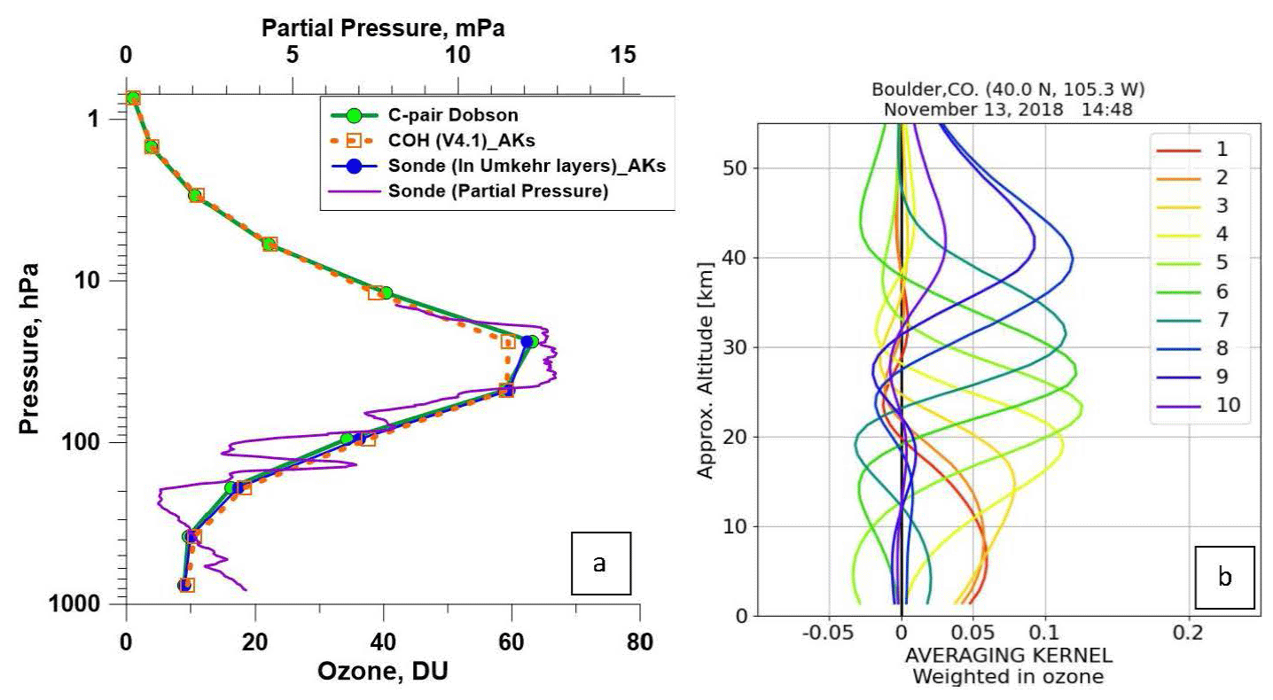
Figure A1(a) An example of ozone observations over the Boulder, CO, station. The purple line is 100 m averaged ozone partial pressure (hPa) vertical profile measured by sonde on 13 November 2018. The green line with solid circles is the ozone profile derived from Dobson Umkehr observations on the same day. The blue line with blue dots is the ozonesonde profile converted to the Umkehr layers and smoothed with the Umkehr AK. The dashed orange line with open squares is the COH ozone profile observed over Boulder on the same day and interpolated to the Umkehr layer vertical grid. (b) The Umkehr AK for the ozone profile was derived from observations in Boulder on 13 November 2018. Each line represents the smoothing function for one of 10 Umkehr layers (see color legend).
Figure A3 demonstrates the time series of monthly mean ground-based records the lower stratosphere at five stations. The Umkehr data (blue) are compared with the ozonesonde anomalies either interpolated to the Umkehr layer 3 (green) or ozonesonde profiles matched with Umkehr profiles in time and smoothed using the Umkehr averaging kernels (crimson). All three datasets have been deseasonalized using their respective climatological (using 1998–2008 climatology) average monthly mean ozone. The application of the averaging kernels has the effect of smoothing the temporal variability.
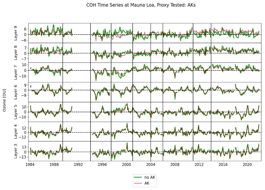
Figure A2Modified residuals (seasonal cycle, solar, QBO, and ENSO are removed, but the trend is retained) of COH overpass data at Mauna Loa (19.5° N, 155.6° W). Red is the layers of AK smoothed to Umkehr; green is the layers that are interpolated to Umkehr. Vertical lines show the dates of satellite records in COH. The largest impact of the AK is seen between 1997 and 2001 where two curves separate in layers 7, 8, and 9 and also after 2001 in layer 9.
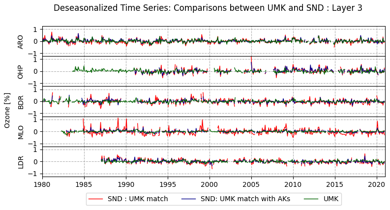
Figure A3Time series of monthly averaged and deseasonalized (in %) ozone anomalies of Umkehr (green) and ozonesonde records are compared at five ground-based stations. Ozonesonde data are either calculated using only profiles that are interpolated in Umkehr layer 3 (blue) or matched with the Umkehr profile in time and smoothed with the Umkehr averaging kernels (crimson).
OMPS SNPP v4r1 uses updated sensor data records (SDRs) as input which incorporate unified and consistent calibration algorithms removing artificial jumps caused by operational changes, instrument anomalies, or contamination for anomaly views of the environment or spacecraft. Also included are new interpolated bandpasses and updated soft calibration based on the newly input SDRs.
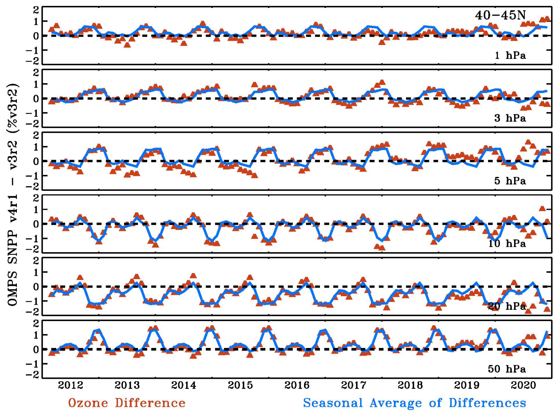
Figure B1Differences in the COH monthly average zonal product as generated from SNPP v4r1 and v3r2 processing. Also shown is the annual cycle in this difference as depicted by the average over all years for each month. Exhibited at 40–45° N is a less than 2 % difference with an annual cycle. A somewhat different pattern is seen in 2020, where the soft calibration for v3r2 is extended beyond its period of relevance.
Differences between the v3r2 and v4r1 versions of the resulting COH dataset are typically less than 1 % (Figs. B1 and B2). Small seasonal variation is apparent at all levels. Larger differences are visible in 2020 when the soft calibration for v3r2 is extended beyond its period of relevance. Figure B3 shows the drift between the two versions. The drift between the datasets is less than ±1 % at all levels. This is a reasonable estimate of the resulting expected trend difference in using the newest COH version compared to the v3r2 results used in Godin-Beekmann et al. (2022).
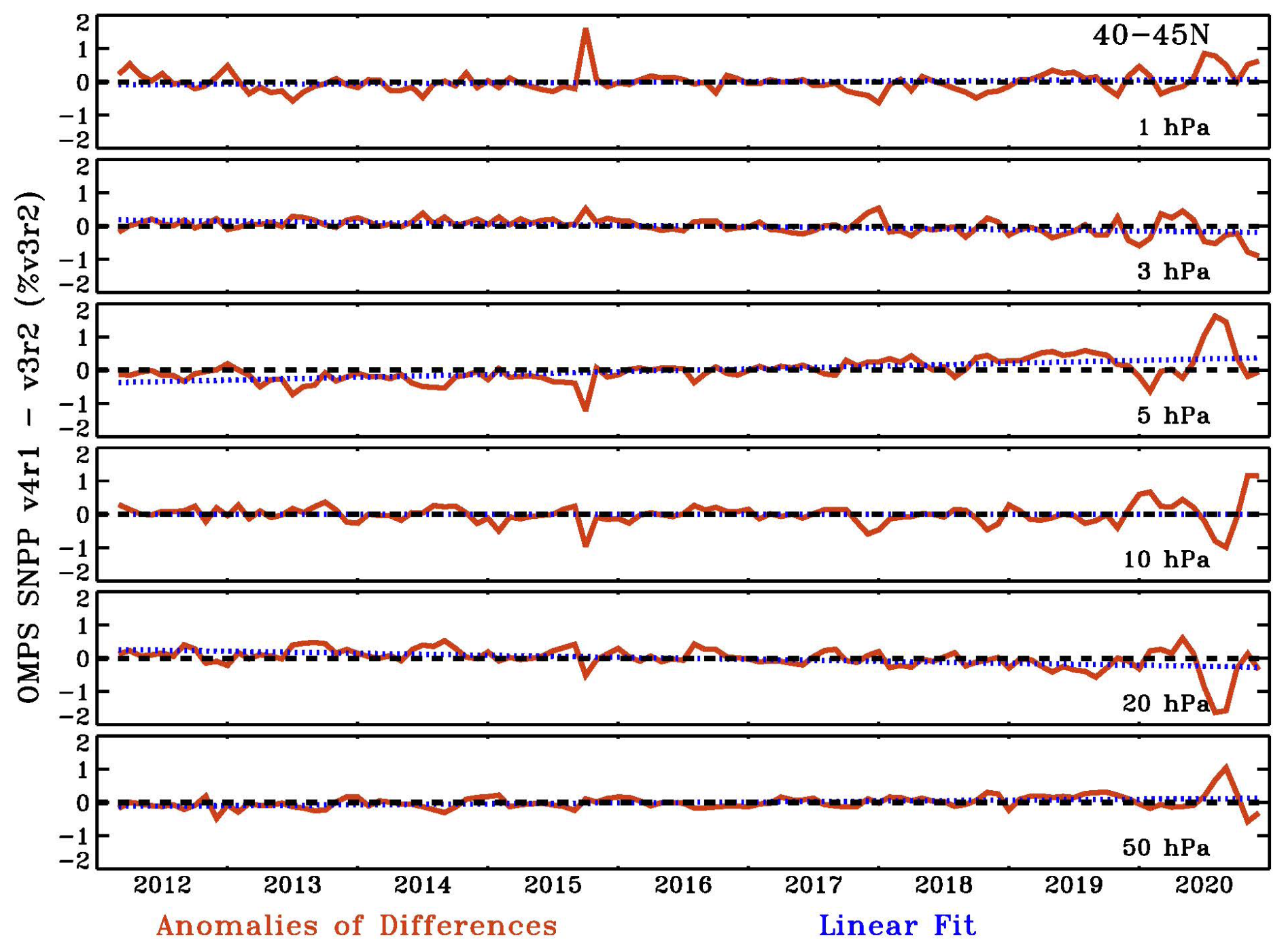
Figure B2Anomalies of the differences in version (v4r1 vs. v3r2) in the COH monthly average zonal product at 40–45° N. Anomalies are enhanced in 2020. Also shown as a dotted blue line is a linear least square fit to the anomalies representing the drift between the two versions.
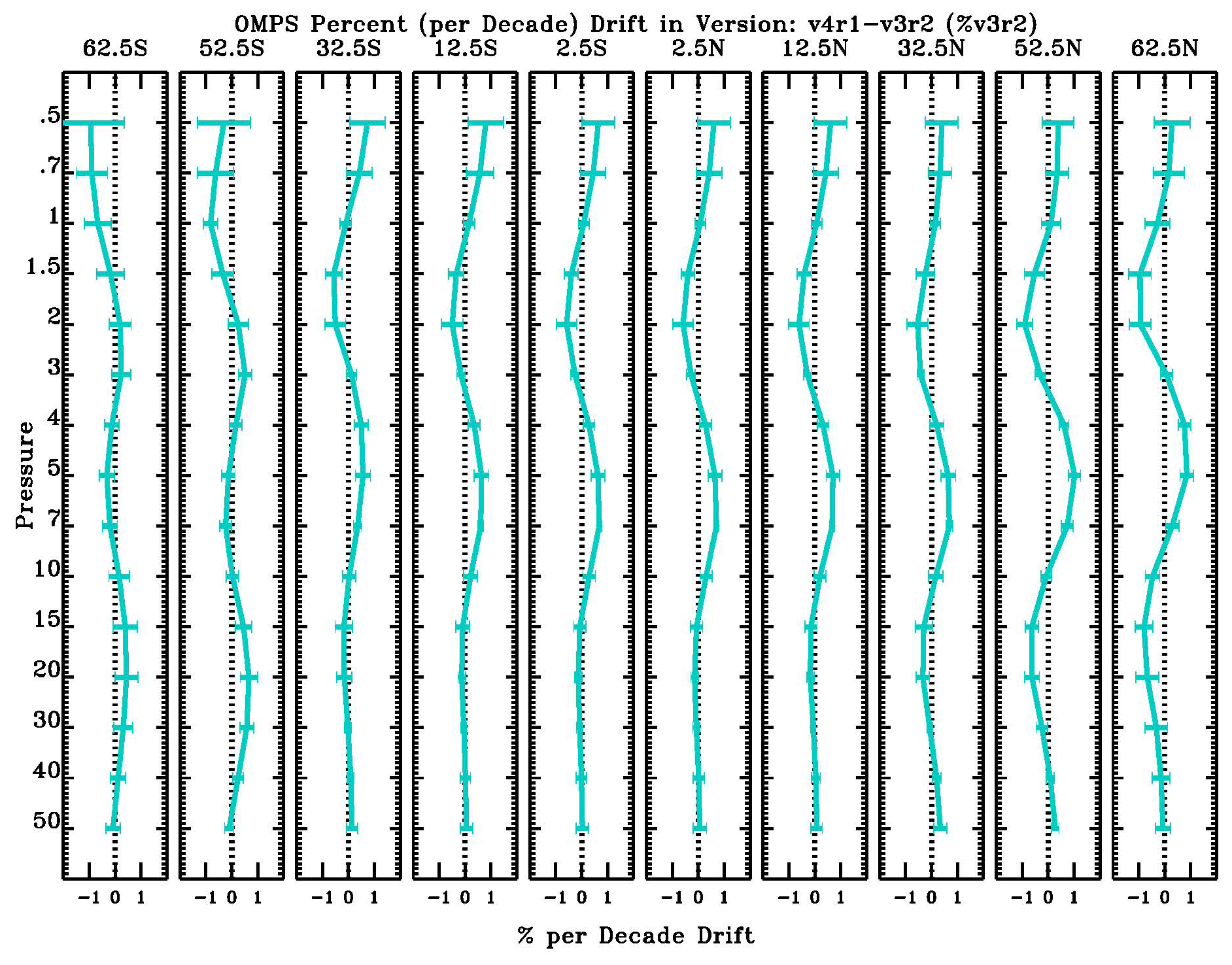
Figure B3The drift between the two versions (v4r1 vs. v3r2) as a function of the pressure level at 10 latitudes.
The COH overpass data used in this paper collect all profiles during the day within a latitude and longitude box of ±2° × ±20° and then generate an inverse-distance-averaged value for the station. The box is based on geometric latitude and longitude. With 15 orbits per day, the chosen box size guarantees two to four possible profiles within the box, depending on whether the orbit overpasses or straddles the site as shown in Fig. C1. Also shown is a scenario in which the equivalent latitude (EqLat) near the site is particularly non-zonal. In such cases, the profiles selected using a geometric coordinate box will select SBUV profiles from an EqLat that are different from that of the measurement station.
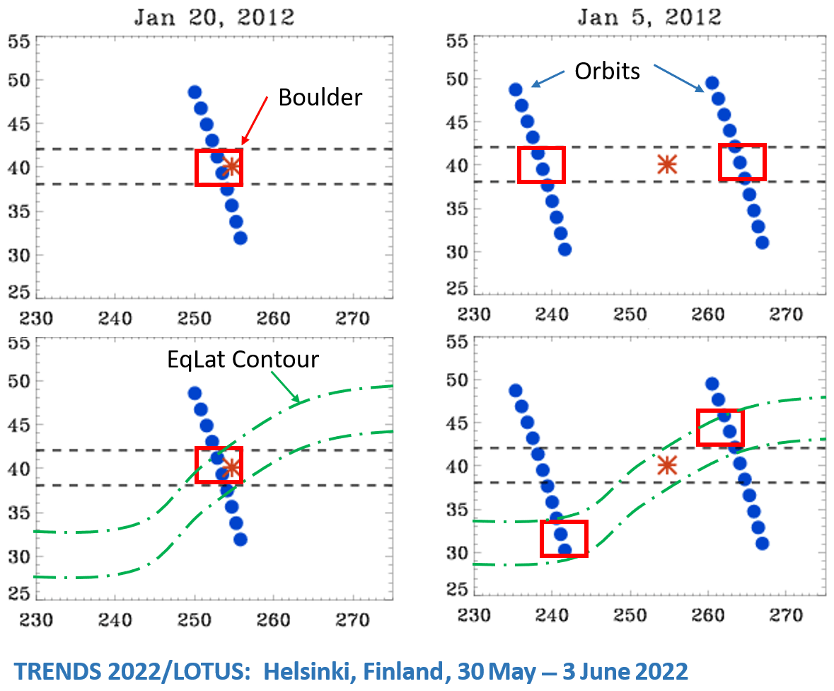
Figure C1Shows orbits of SNPP and positions of OMPS NP ozone profiles on 20 and 5 January 2012. The second row displays a possible EqLat contour overlaid.
It is informative to create an overpass product using boxes based on EqLat and determine the impact on the data. Since EqLat is layer-dependent, the included profiles must be selected independently for each layer. Figure C2 shows COH overpass data for Boulder using geometric coordinates, EqLat-based coordinates, and the associated Umkehr data. Color coding shows the EqLat at Boulder for each measurement day, with dark blue and yellow indicating days with extreme variation from 40° N.
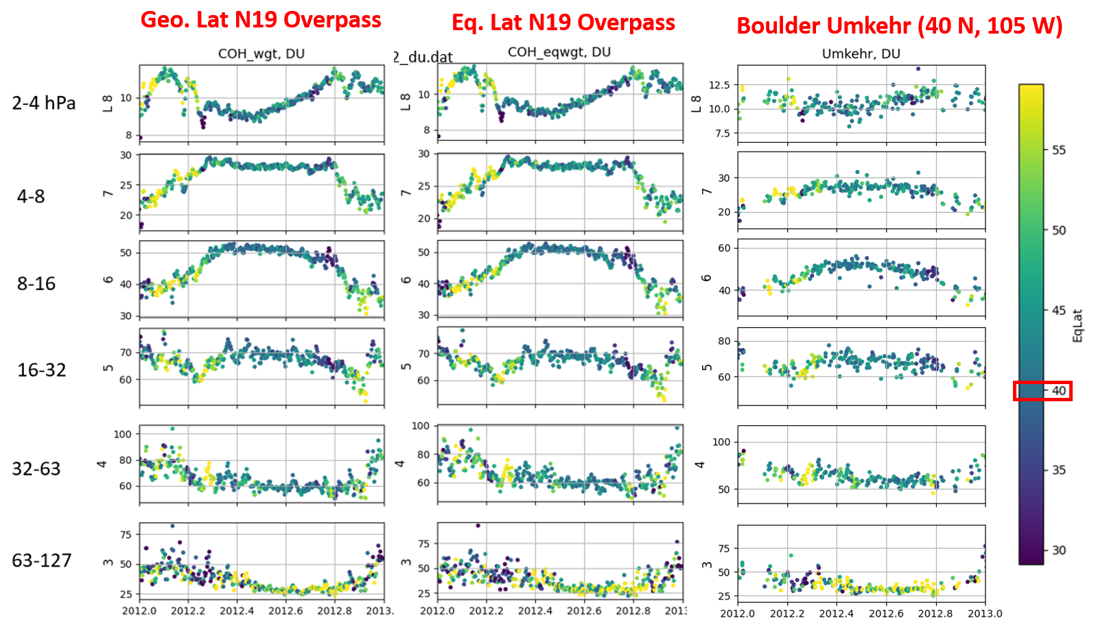
Figure C2COH overpass data were generated with geometric coordinates, EqLat-based coordinates, and the associated Umkehr dataset at Boulder for 2012. Data points are color-coded for the EqLat at the measurement site. Boulder is at 40° N.
The variation in EqLat is most apparent in winter months and transitional fall and spring but less so in summer. Yet the value of the COH ozone is not dramatically altered in the time series. Figure C3 shows correlation plots of the COH overpass to Umkehr for the data at layer 7 (4–8 hPa). The pattern of the scatter and the value of the correlation coefficient are not substantially altered for overpass determination using geometric latitude (left) and EqLat (right). Figure C4 shows the vertical distribution of the correlation coefficient and the RMSE difference for the two COH datasets vs. Umkehr. These two metrics are minimally impacted for this sample year in the layers where COH is valid.
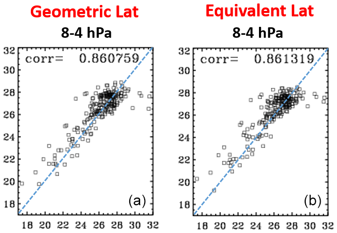
Figure C3Correlation between Umkehr and COH overpass using geometric latitude (a) and EqLat (b) to select included profiles for layer 7 (4–8 hPa).
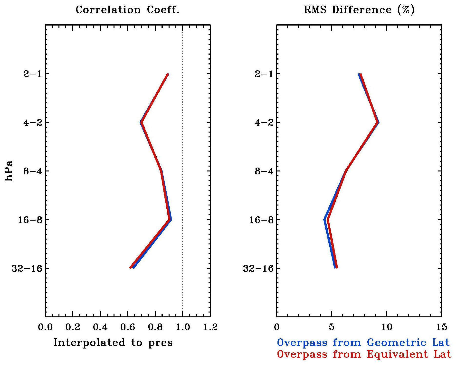
Figure C4Profiles of correlation coefficients and RMSE differences between COH overpass data at Boulder for 2012 using geometric latitude (blue) and EqLat (red) to select data points included in the average. Umkehr data are interpolated to the COH pressure (“pres”) levels.
The use of geometric latitude appears to be sufficient for the choice of included data points in the overpass COH product at the layers used in this paper. This is likely a ramification of the smooth horizontal resolution of the satellite product.
This paper compares trends for three instrument types each with differing measurement frequencies. From each set of measurements, a monthly average is constructed. See the data files at https://doi.org/10.15138/1FF4-HC74 (Miyagawa et al., 2024) for the data and the number of data points in each monthly average with the sampling variations. Umkehr measures once or twice per day, depending on cloud interference with the measurement. At Arosa/Davos and Lauder, Umkehr measurements are sparser than the other GB stations, often taking fewer than 10 measurements per month. At Boulder, beginning in 1983, measurements number 20 or more per month. At OHP, the Umkehr record begins in 1983 with a strong number of 20 or more measurements per month. From 1999 to 2016, however, measurements per month are often fewer than 15. The Umkehr measurements at MLO are the most abundant, especially after 1985, with measuring multiple times a day, resulting in 50–70 data points contributing to the monthly average. The COH overpass dataset is typically available once per day at each station with occasional misses, contributing usually 27–30 data points per month. Since Umkehr can measure multiple times per day, the COH data matched to Umkehr can contain more profiles in the monthly average than the original full COH data, since the COH overpass data will appear twice in the monthly average and once for each Umkehr measurement. This occurs often at MLO. Ozonesonde launches are typically 1 to 3 times per week, depending on the station. At Arosa/Davos, sonde measurements are typically about 15 per month. Sonde measurements at the other stations usually have approximately five measurements per month, with some periods of up to 10 per month. As with COH overpass measurements, the sonde dataset matched to Umkehr can have more contributions to the monthly average resulting from dates with more than one Umkehr measurement, resulting in multiple sonde matches.
The trend results in this paper use all available Umkehr data to generate the monthly means. The COH and sonde data are matched to Umkehr to use the Umkehr temporal sampling for COH and to be able to use the Umkehr averaging kernels for sonde. It is important to determine how the temporal sampling within the monthly mean data may impact trend results. To aid this understanding, we create three subsets of Umkehr data each with different temporal sampling, and we create the corresponding monthly mean, namely (1) all observations in the Umkehr record, (2) Umkehr matched to the COH dataset, and (3) Umkehr matched to the sonde dataset. In this way, we use the same data but only vary the temporal sampling. Since the COH is measured every day, except in the rare case that the satellite data are missing due to instrument issues, sampling (1) and (2) should provide nearly identical results. We expect a strong change in the monthly mean and resulting trends for the Umkehr record when it is matched with an infrequent sampling of ozonesonde profiles (especially in Boulder, Hilo, and Lauder).
Figure D1 summarizes the results. Each line in Fig. D1 is a trend derived from Umkehr data but with sampling of all data, data matched to COH dates, and data matched to sonde dates. In general, the differences are within the envelope of trend uncertainty (±2 SEs). As expected, the trends and standard errors for all (green) and COH-matched subsampled (orange) Umkehr records are nearly the same. The largest differences in all Umkehr and COH-matched Umkehr lines are apparent at OHP. We have determined that this arises from occasional months when there is a short satellite outage coupled with sparse Umkehr observations at the station. However, trends derived from sonde-matched Umkehr data (blue) show deviations from other observations. This is especially clear at Arosa/Davos in the upper stratosphere (∼ 2 %–3 % above 10 hPa). But since this is above the measurement capability of the ozonesonde, it will not impact the ozonesonde trend results at Arosa/Davos. At Lauder, the most significant differences are seen in layer 3 (2.5 %) but unfortunately not in the direction to explain sonde differences in the Lauder trend curves compared to Umkehr. Smaller differences are seen at other layers (very small, less than 1 %, differences in layers 6 and 4). At OHP, small differences of less than 1 % are seen between 50 and 10 hPa, which are well within the error estimates.
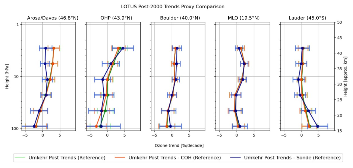
Figure D1Trend results for the reference model using Umkehr data mimicking the temporal sampling of COH and sonde. Green is all available Umkehr data; orange is Umkehr data matched to COH measurement dates; blue is Umkehr data matched to sonde measurement dates.
Figure D2 further explores sampling differences by an examination of trends of COH data using the full COH dataset and data sampled to the Umkehr dates in the generation of the monthly mean datasets. As with Fig. D1, the trend lines are nearly identical at all stations except OHP. At OHP in the early 2000s, there were significantly fewer COH points matched to Umkehr because of the drop in Umkehr measurements. This likely impacts the post-2000 trend estimate. The differences remain below 2 % and are within the error estimate of the trends. In summary, the sampling biases between COH overpass and Umkehr data cannot explain the difference in the derived trends (see Fig. 3; most notable in layers 7 and 8 at Boulder and Lauder).
Figure D3 explores the impact on trends from sampling differences in the sonde data. Shown are trends with all sonde data and trends with Umkehr-matched data. In this figure only, the sonde data are not AK-smoothed since the Umkehr AKs are only available on dates when there is an Umkehr measurement. Shown here are trends from sonde data integrated into the Umkehr levels. As with Fig. D1, the only visible impact is seen at OHP and Lauder, though both are within error estimates. At Lauder, the trends remain negative for both samplings, but the sonde sampled to Umkehr moves closer to the zero line. At OHP, the sonde trends are positive, but the sonde sampled to Umkehr moves slightly closer to zero. The sampling impact on trends for OHP and Lauder is likely due to the reduced number of Umkehr data at these sites.
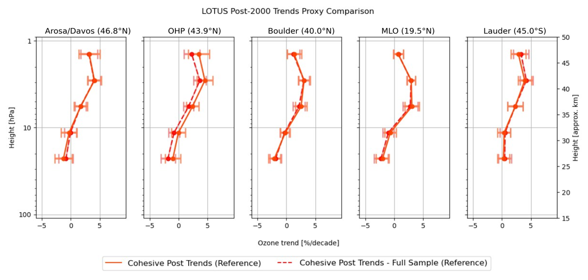
Figure D2Trend results for the reference model exploring variations in the sampling of the COH data. Solid orange is COH data matching Umkehr sampling; dotted orange is all available COH data.
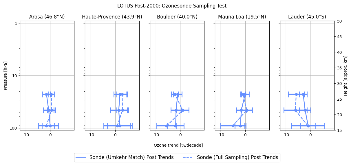
Figure D3Trend results for reference model exploring the sampling of the sonde data. Solid blue is all sonde data; dashed is Umkehr-matched sonde data.
Figure D4 explores the impact of sampling on the adjusted R2 using the COH overpass data. Shown are the adjusted R2 for all available COH overpass data and the same using only COH overpass with matches to the Umkehr data. For Arosa/Davos, OHP, and Lauder, the differences are small. For Boulder and MLO at some layers (Boulder: layers 6, 7; MLO: layers 6, 9), the impact is more apparent, with the full COH exhibiting higher adjusted R2 at these stations.
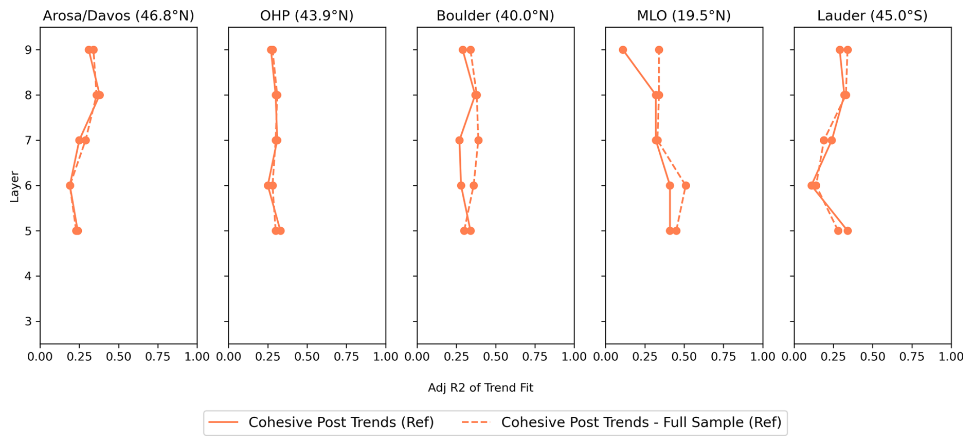
Figure D4Adjusted R2 for the reference model exploring variations in sampling of the COH data. Solid orange is COH data matching Umkehr sampling; dotted orange is all available COH data.
The LOTUS-styled reference model is developed and optimized for zonal average datasets. The extended model tests the addition of single predictors to see if fit statistics can be improved for GB and overpass datasets. For tropospheric pressure (TP), improvements are consistent among layers and among instrument types. The addition of EqLat also yields consistent results for instrument types and at most stations, though not Mauna Loa. The addition of other predictors gives mixed results, depending on the level and station. The potential for improving confidence in the trend result exists by combining predictors using different choices, depending on the layer and station. We choose additional predictor combinations with the consideration of three criteria: (1) combined predictors should not have a high correlation with each other (usually 0.2 or less), (2) predictors should reduce the SEs of the trend consistently for all instrument types, and (3) the addition of the predictor should not greatly reduce the adjusted R2 of the model fit but preferentially increase it. As seen in Table 7e and f, the NAO and the EHF predictors do not make a significant improvement when added to the reference model, so we do not include either in the full model.
E1 Mixed model
We have noted a high correlation between the TP and EqLat predictors at all levels, especially for Boulder, Mauna Loa, and Lauder with correlation adjusted R2 of 0.4 to 0.7 and somewhat less correlated at Arosa/Davos and OHP with adjusted R2 of 0.2 and 0.3. Subsequently, we choose to not use these two predictors together (at the same station/layer combination). The addition of TP at all stations for layers 3 and 4 uniformly decreases the standard errors at all stationsfor Umkehr and sonde. The addition of EqLat (with the exception of Umkehr at Boulder; level 5) almost uniformly decreases the standard errors at all stations for layers 5 and 6. There is an additional reduction in the SEs for layers 7 to 9 for all stations, except at Mauna Loa. Thus, we choose TP and EqLat as additional predictors at these layers. QBO C and D have significant impact in decreasing the SEs in layers 4 and 5 for both Umkehr and sonde and layer 3 for sonde, with only a small degradation for Umkehr. QBO CD shows an improvement in layer 8 at OHP for COH and Umkehr and Arosa/Davos and Boulder for COH only. We have tested adding QBO and EqLat for layer 8 at these three stations. For Umkehr measurements, there is no improvement beyond EqLat only with QBO CD also included. For COH, there is additional improvement but not to the extent of QBO CD alone. Since the improvement is limited to one layer, and for only COH, we choose to only add the additional QBO CD for the tropical MLO. Table E1 shows the resulting combination of additional predictors for this mixed model.
Table E1Details of additional predictor combinations for each level and station in the mixed model.
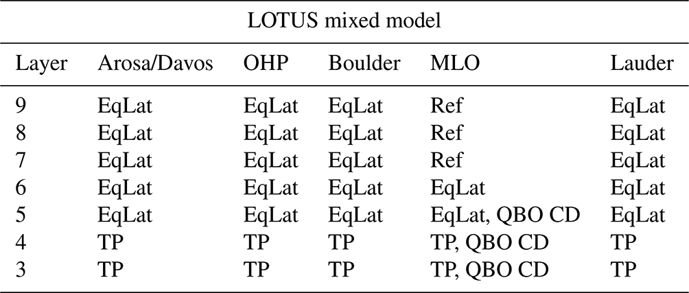
The resulting change in SEs from the reference model is shown in Table E2. For most stations/layers, this is simply a composite of the values from the single EqLat or TP extended model results. There remain a few instrument/station/layers in which the SEs are slightly increased – Arosa/Davos Umkehr layer 8 and Boulder Umkehr layer 8 – but these are negligible. At Boulder layer 5 Umkehr, the increase in SEs is somewhat more at 1.85 % difference, but this is still small enough to not be of great concern. For Mauna Loa at layers 3, 4, and 5, the model is rerun adding two predictors together, and the results are new. Indeed, in these cases, the SEs are improved beyond the single predictor results of either QBO alone or TP or EqLat alone, with the exception of Sonde layer 5, where the change in SEs is just slightly degraded from QBO alone (13.42 % vs. 13.69 % reduction in SEs).
Table E3 shows the adjusted R2 for the proposed mixed models. Similar to the change in SEs (Table E2), the adjusted R2 is a composite of the individual EqLat or TP results from the extended model, with the exception of the results for layers 3, 4, and 5 at Mauna Loa, where both predictors are included concurrently. At these layers, the adjusted R2 (Adj R2) in some cases matches the higher Adj R2 values of the two predictors and in others improves with the combination of QBO and TP or EqLat.
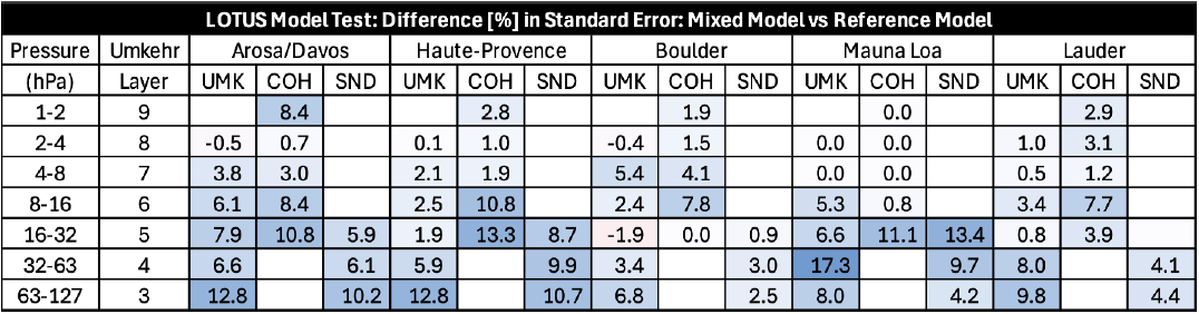
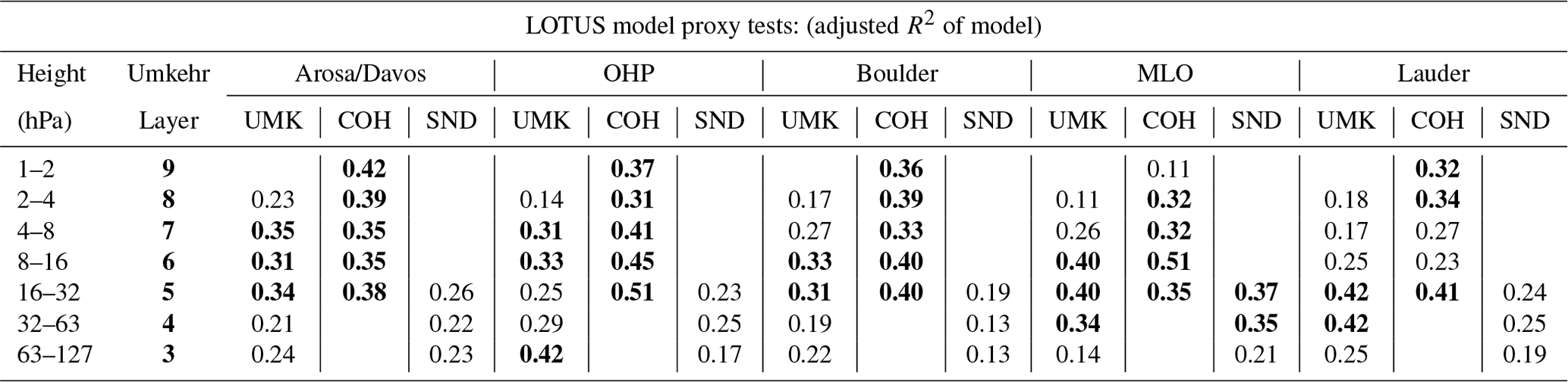
E2 Augmented mixed model
It is hard to ignore the substantial reduction in SEs when adding the AO/AAO predictor, especially for layers 3, 4, and 5 at Mauna Loa and for layers 3 and 4 at Arosa/Davos. The results for OHP layers 3 and 4 are still compelling, though somewhat less so. So we explore the addition of AO/AAO at these three stations only for the layers specified. Table E4 summarizes the predictor choices for this augmented mixed model.
Table E5 displays the change in the SEs from the reference model now for the augmented mixed model. Adding AO/AAO at Arosa/Davos (layers 3 and 4) and Mauna Loa (layers 3 to 5) greatly reduces the SEs beyond that of the mixed model results in Table E2. For OHP (layers 3 and 4), the impact is less dramatic for Umkehr. For sonde measurements at layer 4, the AO/AAO addition has no impact beyond the mixed model; for layer 3, the addition of AO/AAO results in less of a reduction in the SEs.
Table E4Details of additional predictor choices for each level and station in the augmented mixed model. This differs from Table A1 by adding AO/AAO at some levels for Arosa/Davos, OHP, and Mauna Loa.
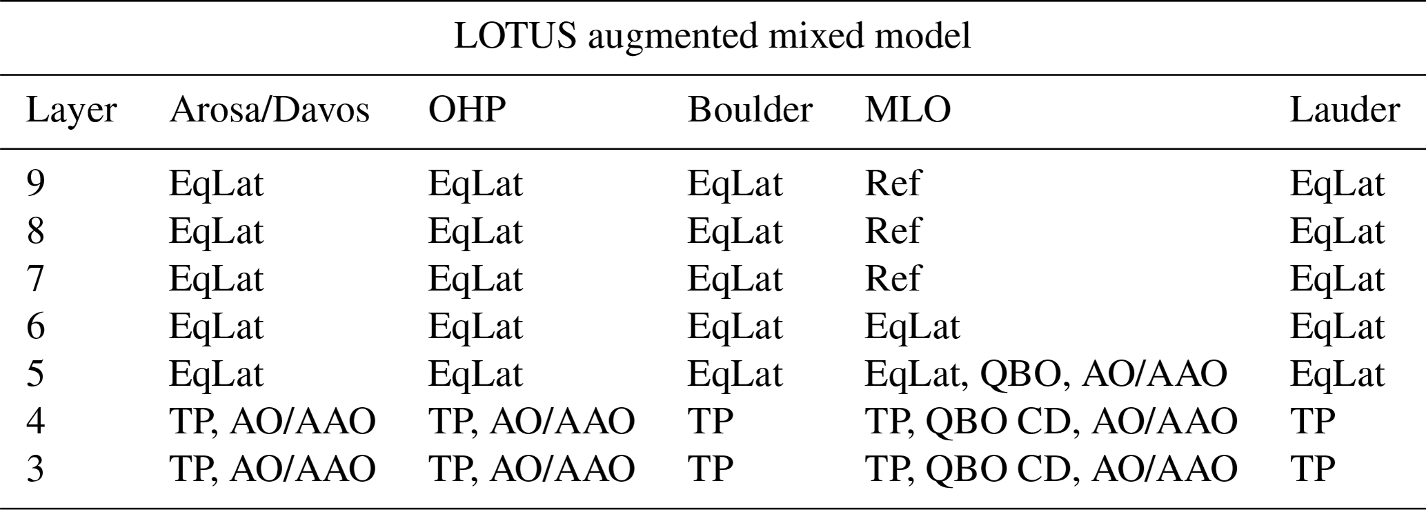
Table E5The same as Table 9. Change in the SEs of the trend using the augmented mixed model.
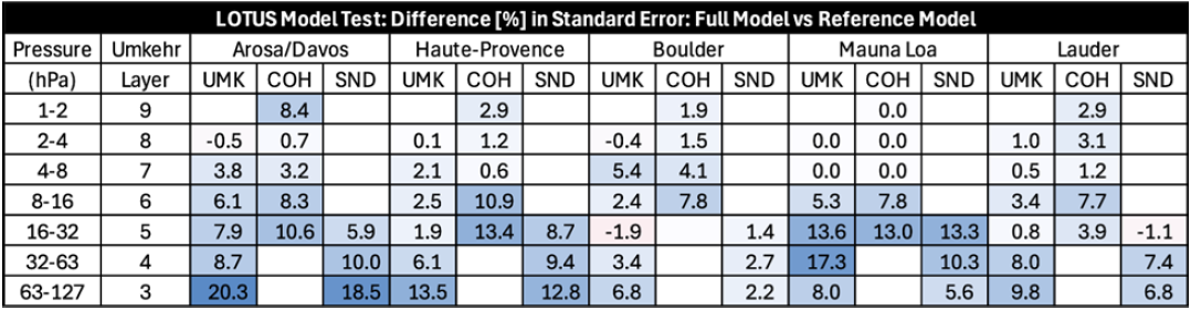
Table E6 displays the Adj R2 for the augmented mixed model. Adding AO/AAO improves the Adj R2 results for Arosa/Davos and MLO and has little to no impact at OHP. Based on the criteria outlined at the beginning of this Appendix, we assign the augmented mixed model to the “full model” in the body of this paper.
Table E6The same as Table 12 with adjusted R2 for the augmented mixed model.
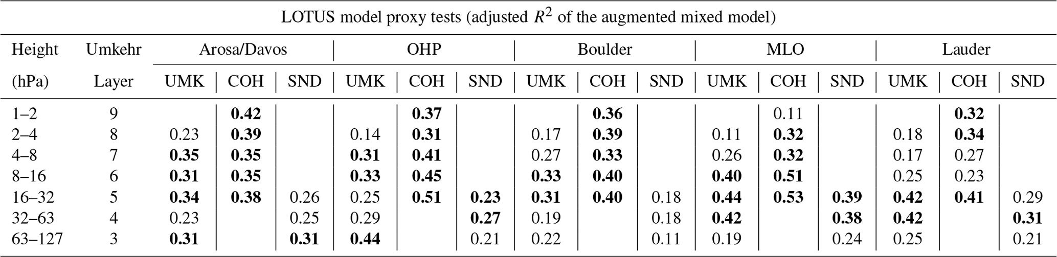
All datasets used in this study are publicly available from https://doi.org/10.15138/1FF4-HC74 (Miyagawa et al., 2024).
IP and JW conceptualized the paper, and IP led the paper preparation. PE, KA, and JW performed the data analysis. KM was responsible for the production of the spatial and temporally matched ground-based and satellite ozone profile data. JW was responsible for producing COH zonally averaged and station overpass ozone profile records. LF was responsible for the retrieval and calibration of the OMPS data. GM, PE, KM, and KA were responsible for the NOAA Umkehr measurements. EMB was responsible for measurements in Arosa/Davos. RQ was responsible for Umkehr and ozonesonde observations in Lauder, Aotearoa / New Zealand. BJ and PC were responsible for ozonesonde observations in Boulder and Hilo. GA was responsible for the ozonesonde observations in OHP. RVM was responsible for HEGIFTOM ozonesonde records and data analyses. RD, SGB, and DZ provided the context for the LOTUS model use and interpretation of trend analyses. All authors contributed to the writing of the paper.
The contact author has declared that none of the authors has any competing interests.
The statements, findings, conclusions, and recommendations are those of the author(s) and do not necessarily reflect the views of NOAA or the U.S. Department of Commerce.
Publisher's note: Copernicus Publications remains neutral with regard to jurisdictional claims made in the text, published maps, institutional affiliations, or any other geographical representation in this paper. While Copernicus Publications makes every effort to include appropriate place names, the final responsibility lies with the authors.
This study has been supported in part by NOAA (grant no. NA19NES4320002; Cooperative Institute for Satellite Earth System Studies – CISESS) at the University of Maryland/ESSIC and NOAA (grant no. NA22OAR4320151) for the Cooperative Institute for Earth System Research and Data Science (CIESRDS). Additional funding has been provided by NOAA Climate Program Office's Atmospheric Chemistry, Carbon Cycle, and Climate program (AC4) (grant nos. NA19OAR4310169 (CU)/NA19OAR4310171(UMD)).
The authors would like to thank the NASA/GSFC Atmospheric Chemistry and Dynamics team for the SBUV/2 v8.6 profile data; Eric Beach from the NESDIS/STAR for his help with the Suomi National Polar-orbiting Partnership (SNPP) OMPS data; the NOAA GML observatory team (Boulder, MLO, and Fairbanks observatories), LATMOS (OHP), and NIWA (Lauder) for Umkehr and ozonesonde data; Wolfgang Steinbrecht of the DWD for help with interpretation of the Hohenpeißenberg ozonesonde data; and the MeteoSwiss and PMOD/WRC teams (Arosa/Davos) for Dobson Umkehr data. Some data are associated with the Network for the Detection of Atmospheric Composition Change (NDACC) and are available through the NDACC website (https://www.ndacc.org/, last access: 1 June 2024). The authors extend their thanks to Susan Strahan for the equivalent latitude data at each station, to Kai-Lan Chang of CIRES for the discussion of the statistical interpretation of the thresholds, and to Justin Alsing for the development of the LOTUS code. North American Regional Reanalysis (NARR) data were provided by the NOAA PSL, Boulder, Colorado, USA, from their website at https://psl.noaa.gov/ (last access: 1 June 2024).
This research has been supported in part by NOAA (grant no. NA19NES4320002; Cooperative Institute for Satellite Earth System Studies – CISESS) at the University of Maryland/ESSIC and NOAA (grant no. NA22OAR4320151) for the Cooperative Institute for Earth System Research and Data Science (CIESRDS). Additional funding has been provided by NOAA Climate Program Office's Atmospheric Chemistry, Carbon Cycle, and Climate program (AC4) (grant nos. NA19OAR4310169 (CU)/NA19OAR4310171(UMD)).
This paper was edited by Jayanarayanan Kuttippurath and reviewed by two anonymous referees.
Anstey, J. A., Banyard, T. P., Butchart, N., Coy, L., Newman, P. A., Osprey, S., and Wright, C. J. : Prospect of increased disruption to the QBO in a changing climate, Geophys. Res. Lett., 48, e2021GL093058, https://doi.org/10.1029/2021GL093058, 2021.
Ancellet, G., Godin-Beekmann, S., Smit, H. G. J., Stauffer, R. M., Van Malderen, R., Bodichon, R., and Pazmiño, A.: Homogenization of the Observatoire de Haute Provence electrochemical concentration cell (ECC) ozonesonde data record: comparison with lidar and satellite observations, Atmos. Meas. Tech., 15, 3105–3120, https://doi.org/10.5194/amt-15-3105-2022, 2022.
Bai, K., Liu, C., Shi, R., and Gao, W.: Comparison of Suomi-NPP OMPS total column ozone with Brewer and Dobson spectrophotometers measurements, Frontiers of Earth Science, 9, 369–380, https://doi.org/10.1007/s11707-014-0480-5, 2015.
Ball, W. T., Chiodo, G., Abalos, M., Alsing, J., and Stenke, A.: Inconsistencies between chemistry–climate models and observed lower stratospheric ozone trends since 1998, Atmos. Chem. Phys., 20, 9737–9752, https://doi.org/10.5194/acp-20-9737-2020, 2020.
Bernet, L., Svendby, T., Hansen, G., Orsolini, Y., Dahlback, A., Goutail, F., Pazmiño, A., Petkov, B., and Kylling, A.: Total ozone trends at three northern high-latitude stations, Atmos. Chem. Phys., 23, 4165–4184, https://doi.org/10.5194/acp-23-4165-2023, 2023.
Bhartia, P. K., Herman, J. R., McPeters, R. D., and Torres, O.: Effect of Mount Pinatubo aerosols on total ozone measurements from backscatter ultraviolet (BUV) experiments, J. Geophys. Res., 98, 18547–18554, https://doi.org/10.1029/93JD01739, 1993.
Bhartia, P. K., McPeters, R. D., Flynn, L. E., Taylor, S., Kramarova, N. A., Frith, S., Fisher, B., and DeLand, M.: Solar Backscatter UV (SBUV) total ozone and profile algorithm, Atmos. Meas. Tech., 6, 2533–2548, https://doi.org/10.5194/amt-6-2533-2013, 2013.
Björklund, R., Vigouroux, C., Effertz, P., García, O. E., Geddes, A., Hannigan, J., Miyagawa, K., Kotkamp, M., Langerock, B., Nedoluha, G., Ortega, I., Petropavlovskikh, I., Poyraz, D., Querel, R., Robinson, J., Shiona, H., Smale, D., Smale, P., Van Malderen, R., and De Mazière, M.: Intercomparison of long-term ground-based measurements of total, tropospheric, and stratospheric ozone at Lauder, New Zealand, Atmos. Meas. Tech., 17, 6819–6849, https://doi.org/10.5194/amt-17-6819-2024, 2024.
Boynard, A., Hurtmans, D., Garane, K., Goutail, F., Hadji-Lazaro, J., Koukouli, M. E., Wespes, C., Vigouroux, C., Keppens, A., Pommereau, J.-P., Pazmino, A., Balis, D., Loyola, D., Valks, P., Sussmann, R., Smale, D., Coheur, P.-F., and Clerbaux, C.: Validation of the IASI FORLI/EUMETSAT ozone products using satellite (GOME-2), ground-based (Brewer–Dobson, SAOZ, FTIR) and ozonesonde measurements, Atmos. Meas. Tech., 11, 5125–5152, https://doi.org/10.5194/amt-11-5125-2018, 2018.
Chang, K.-L., Cooper, O. R., Gaudel, A., Petropavlovskikh, I., and Thouret, V.: Statistical regularization for trend detection: an integrated approach for detecting long-term trends from sparse tropospheric ozone profiles, Atmos. Chem. Phys., 20, 9915–9938, https://doi.org/10.5194/acp-20-9915-2020, 2020.
Chang, K. L., Schultz, M. G., Lan, X., McClure-Begley, A., Petropavlovskikh, I., Xu, X., and Ziemke, J. R.: Trend detection of atmospheric time series: Incorporating appropriate uncertainty estimates and handling extreme events, Elementa: Science of the Anthropocene, 9, 00035, https://doi.org/10.1525/elementa.2021.00035, 2021.
Chang, K.-L., Schultz, M. G., Koren, G., and Selke, N.: Guidance note on best statistical practices for TOAR analyses, TOAR tropospheric ozone assessment report, https://igacproject.org/sites/default/files/2023-04/STAT_recommendations_TOAR_analyses_0.pdf (last access: 12 July 2023), 2023.
Chang, K.-L., Cooper, O. R., Gaudel, A., Petropavlovskikh, I., Effertz, P., Morris, G., and McDonald, B. C.: Technical note: Challenges in detecting free tropospheric ozone trends in a sparsely sampled environment, Atmos. Chem. Phys., 24, 6197–6218, https://doi.org/10.5194/acp-24-6197-2024, 2024.
Cochrane, D. and Orcutt, G. H.: Application of least squares regression to relationships containing auto-correlated error terms, J. Am. Stat. Assoc., 44, 32–61, https://doi.org/10.1080/01621459.1949.10483290, 1949.
DeLuisi, J. J., Longenecker, D. U., Mateer, C. L., and Wuebbles, D. J.: An analysis of northern middle-latitude Umkehr measurements corrected for stratospheric aerosols for 1979–1986, J. Geophys. Res., 94, 9837–9846, https://doi.org/10.1029/JD094iD07p09837, 1989.
Diallo, M., Riese, M., Birner, T., Konopka, P., Müller, R., Hegglin, M. I., Santee, M. L., Baldwin, M., Legras, B., and Ploeger, F.: Response of stratospheric water vapor and ozone to the unusual timing of El Niño and the QBO disruption in 2015–2016, Atmos. Chem. Phys., 18, 13055–13073, https://doi.org/10.5194/acp-18-13055-2018, 2018.
Diallo, M. A., Ploeger, F., Hegglin, M. I., Ern, M., Grooß, J.-U., Khaykin, S., and Riese, M.: Stratospheric water vapour and ozone response to the quasi-biennial oscillation disruptions in 2016 and 2020, Atmos. Chem. Phys., 22, 14303–14321, https://doi.org/10.5194/acp-22-14303-2022, 2022.
EEAP (Environmental Effects Assessment Panel): 2022 Quadrennial Assessment – Environmental effects of stratospheric ozone depletion, UV radiation, and interactions with climate change, https://ozone.unep.org/system/files/documents/EEAP-2022-Assessment-Report-May2023.pdf (last access: 5 March 2024), 2023.
Evans, R. D., Petropavlovskikh, I., McClure-Begley, A., McConville, G., Quincy, D., and Miyagawa, K.: Technical note: The US Dobson station network data record prior to 2015, re-evaluation of NDACC and WOUDC archived records with WinDobson processing software, Atmos. Chem. Phys., 17, 12051–12070, https://doi.org/10.5194/acp-17-12051-2017, 2017.
Fioletov, V. E. and Shepherd, T. G.: Summertime total ozone variations over middle and polar latitudes, Geophys. Res. Lett., 32, L04807, https://doi.org/10.1029/2004GL022080, 2005.
Fioletov, V. E., Labow, G., Evans, R., Hare, E. W., Köhler, U., McElroy, C. T., Miyagawa, K., Redondas, A., Savastiouk, V., Shalamyansky, A. M., Staehelin, J., Vanicek, K., and Weber, M.: Performance of the ground-based total ozone network assessed using satellite data, J. Geophys. Res., 113, D14313, https://doi.org/10.1029/2008JD009809, 2008.
Frith, S. M., Kramarova, N. A., Stolarski, R. S., McPeters, R. D., Bhartia, P. K., and Labow, G. J.: Recent changes in total column ozone based on the SBUV Version 8.6 Merged Ozone Data Set, J. Geophys. Res.-Atmos., 119, 9735–9751, https://doi.org/10.1002/2014JD021889, 2014.
Frith, S. M., Kramarova, N. A., Bhartia, P. K., McPeters, R. D., Labow, G. J., Ziemke, J. R., and Haffner, D.: Recent Advances in the SBUV Merged Ozone Dataset (MOD) for LOTUS Phase 2 Analysis of Stratospheric Ozone Trends and Uncertainties, in: LOTUS Phase 2 Workshop, Virtual, 28 May 2020, https://acd-ext.gsfc.nasa.gov/People/Frith/webdir/modprof/pubpage/LOTUS_May_28_2020.pdf (last access: 1 June 2024), 2020.
Godin-Beekmann, S., Azouz, N., Sofieva, V. F., Hubert, D., Petropavlovskikh, I., Effertz, P., Ancellet, G., Degenstein, D. A., Zawada, D., Froidevaux, L., Frith, S., Wild, J., Davis, S., Steinbrecht, W., Leblanc, T., Querel, R., Tourpali, K., Damadeo, R., Maillard Barras, E., Stübi, R., Vigouroux, C., Arosio, C., Nedoluha, G., Boyd, I., Van Malderen, R., Mahieu, E., Smale, D., and Sussmann, R.: Updated trends of the stratospheric ozone vertical distribution in the 60° S–60° N latitude range based on the LOTUS regression model, Atmos. Chem. Phys., 22, 11657–11673, https://doi.org/10.5194/acp-22-11657-2022, 2022.
Harris, N. R. P., Hassler, B., Tummon, F., Bodeker, G. E., Hubert, D., Petropavlovskikh, I., Steinbrecht, W., Anderson, J., Bhartia, P. K., Boone, C. D., Bourassa, A., Davis, S. M., Degenstein, D., Delcloo, A., Frith, S. M., Froidevaux, L., Godin-Beekmann, S., Jones, N., Kurylo, M. J., Kyrölä, E., Laine, M., Leblanc, S. T., Lambert, J.-C., Liley, B., Mahieu, E., Maycock, A., de Mazière, M., Parrish, A., Querel, R., Rosenlof, K. H., Roth, C., Sioris, C., Staehelin, J., Stolarski, R. S., Stübi, R., Tamminen, J., Vigouroux, C., Walker, K. A., Wang, H. J., Wild, J., and Zawodny, J. M.: Past changes in the vertical distribution of ozone – Part 3: Analysis and interpretation of trends, Atmos. Chem. Phys., 15, 9965–9982, https://doi.org/10.5194/acp-15-9965-2015, 2015.
Hassler, B., Petropavlovskikh, I., Staehelin, J., August, T., Bhartia, P. K., Clerbaux, C., Degenstein, D., Mazière, M. D., Dinelli, B. M., Dudhia, A., Dufour, G., Frith, S. M., Froidevaux, L., Godin-Beekmann, S., Granville, J., Harris, N. R. P., Hoppel, K., Hubert, D., Kasai, Y., Kurylo, M. J., Kyrölä, E., Lambert, J.-C., Levelt, P. F., McElroy, C. T., McPeters, R. D., Munro, R., Nakajima, H., Parrish, A., Raspollini, P., Remsberg, E. E., Rosenlof, K. H., Rozanov, A., Sano, T., Sasano, Y., Shiotani, M., Smit, H. G. J., Stiller, G., Tamminen, J., Tarasick, D. W., Urban, J., van der A, R. J., Veefkind, J. P., Vigouroux, C., von Clarmann, T., von Savigny, C., Walker, K. A., Weber, M., Wild, J., and Zawodny, J. M.: Past changes in the vertical distribution of ozone – Part 1: Measurement techniques, uncertainties and availability, Atmos. Meas. Tech., 7, 1395–1427, https://doi.org/10.5194/amt-7-1395-2014, 2014.
Hassler, B., Kremser, S., Bodeker, G. E., Lewis, J., Nesbit, K., Davis, S. M., Chipperfield, M. P., Dhomse, S. S., and Dameris, M.: An updated version of a gap-free monthly mean zonal mean ozone database, Earth Syst. Sci. Data, 10, 1473–1490, https://doi.org/10.5194/essd-10-1473-2018, 2018.
Hassler, B., Young, P. (Lead Authors), Ball, W. T., Damadeo, R., Keeble, J., Maillard Barras, E., Sofieva, V., and Zeng, G.: Update on Global Ozone: Past, Present, and Future, Chap. 3 in: Scientific Assessment of Ozone Depletion: 2022, GAW Report No. 278, WMO, Geneva, 278, 154–214, ISBN: 978 9914 733 97 6, 2022.
Hubert, D., Lambert, J.-C., Verhoelst, T., Granville, J., Keppens, A., Baray, J.-L., Bourassa, A. E., Cortesi, U., Degenstein, D. A., Froidevaux, L., Godin-Beekmann, S., Hoppel, K. W., Johnson, B. J., Kyrölä, E., Leblanc, T., Lichtenberg, G., Marchand, M., McElroy, C. T., Murtagh, D., Nakane, H., Portafaix, T., Querel, R., Russell III, J. M., Salvador, J., Smit, H. G. J., Stebel, K., Steinbrecht, W., Strawbridge, K. B., Stübi, R., Swart, D. P. J., Taha, G., Tarasick, D. W., Thompson, A. M., Urban, J., van Gijsel, J. A. E., Van Malderen, R., von der Gathen, P., Walker, K. A., Wolfram, E., and Zawodny, J. M.: Ground-based assessment of the bias and long-term stability of 14 limb and occultation ozone profile data records, Atmos. Meas. Tech., 9, 2497–2534, https://doi.org/10.5194/amt-9-2497-2016, 2016.
Kalnay, E., Kanamitsu, M., Kistler, R., Collins, W., Deaven, D., Gandin, L., Iredell, M., Saha, S., White, G., Woollen, J., Zhu, Y., Chelliah, M., Ebisuzaki, W., Higgins, W., Janowiak, J., Mo, K. C., Ropelewski, C., Wang, J., Leetmaa, A., Reynolds, R., Jenne, R., and Joseph, D.: The NCEP/NCAR 40-year reanalysis project, B. Am. Meteorol. Soc., 77, 437–470, https://doi.org/10.1175/1520-0477(1996)077<0437:TNYRP>2.0.CO;2, 1996.
Knudsen, B. M. and Grooss, J. U.: Northern midlatitude stratospheric ozone dilution in spring modeled with simulated mixing, J. Geophys. Res., 105, 6885–6890, https://doi.org/10.1029/1999JD901076, 2000.
Koukouli, M. E., Zara, M., Lerot, C., Fragkos, K., Balis, D., van Roozendael, M., Allart, M. A. F., and van der A, R. J.: The impact of the ozone effective temperature on satellite validation using the Dobson spectrophotometer network, Atmos. Meas. Tech., 9, 2055–2065, https://doi.org/10.5194/amt-9-2055-2016, 2016.
Kramarova, N. A., Frith, S. M., Bhartia, P. K., McPeters, R. D., Taylor, S. L., Fisher, B. L., Labow, G. J., and DeLand, M. T.: Validation of ozone monthly zonal mean profiles obtained from the version 8.6 Solar Backscatter Ultraviolet algorithm, Atmos. Chem. Phys., 13, 6887–6905, https://doi.org/10.5194/acp-13-6887-2013, 2013a.
Kramarova, N. A., Bhartia, P. K., Frith, S. M., McPeters, R. D., and Stolarski, R. S.: Interpreting SBUV smoothing errors: an example using the quasi-biennial oscillation, Atmos. Meas. Tech., 6, 2089–2099, https://doi.org/10.5194/amt-6-2089-2013, 2013b.
Lary, D. J., Chipperfield, M. P., Pyle, J. A., Norton, W. A. Riishøjgaard, L. P.: Three-dimensional tracer initialization and general diagnostics using equivalent PV latitude–potential-temperature coordinates, Q. J. Roy. Meteor. Soc., 121, 187–210, https://doi.org/10.1002/qj.49712152109, 1995.
Lawrence, Z. D., Perlwitz, J., Butler, A. H., Manney, G. L., Newman, P. A., Lee, S. H., and Nash, E. R.: The remarkably strong Arctic stratospheric polar vortex of winter 2020: Links to record-breaking Arctic Oscillation and ozone loss, J. Geophys. Res.-Atmos., 125, e2020JD033271, https://doi.org/10.1029/2020JD033271, 2020.
Lee, H. and Smith, A. K.: Simulation of the combined effects of solar cycle, quasi-biennial oscillation, and volcanic forcing on stratospheric ozone changes in recent decades, J. Geophys. Res., 108, 4049, https://doi.org/10.1029/2001JD001503, 2003.
Madronich, S., Lee-Taylor, J. M., Wagner, M., Kyle, J., Hu, Z., and Landolfi, R.: Estimation of skin and ocular damage avoided in the United States through implementation of the Montreal Protocol on Substances that Deplete the Ozone Layer, ACS Earth and Space Chemistry, 5, 1876–1888, https://doi.org/10.1021/acsearthspacechem.1c00183, 2021.
Maillard Barras, E., Haefele, A., Stübi, R., Jouberton, A., Schill, H., Petropavlovskikh, I., Miyagawa, K., Stanek, M., and Froidevaux, L.: Dynamical linear modeling estimates of long-term ozone trends from homogenized Dobson Umkehr profiles at Arosa/Davos, Switzerland, Atmos. Chem. Phys., 22, 14283–14302, https://doi.org/10.5194/acp-22-14283-2022, 2022.
Manney, G. L. and Hegglin, M. I.: Seasonal and Regional Variations of Long-Term Changes in Upper-Tropospheric Jets from Reanalyses, J. Climate, 31, 423–448, https://doi.org/10.1175/JCLI-D-17-0303.1, 2018.
Manney, G., Santee, M., Rex, M., Livesey, N. J., Pitts, M. C., Veefkind, P., Nash, E. R., Wohltmann, I., Lehmann, R., Froidevaux, L., Poole, L. R., Schoeberl, M. R., Haffner, D. P., Davies, J., Dorokhov, V., Gernandt, H., Johnson, B., Kivi, R., Kyrö, E., Larsen, N., Levelt, P. F., Makshtas, A., McElroy, C. T., Nakajima, H., Parrondo, M. C., Tarasick, D. W., von der Gathen, P., Walker, K. A., and Zinoviev, N. S.: Unprecedented Arctic ozone loss in 2011, Nature, 478, 469–475, https://doi.org/10.1038/nature10556, 2011.
McPeters, R. D., Bhartia, P. K., Haffner, D., Labow, G. J., and Flynn, L.: The version 8.6 SBUV ozone data record: An overview, J. Geophys. Res. Atmos., 118, 8032–8039, https://doi.org/10.1002/jgrd.50597, 2013.
Meng, L., Liu, J., Tarasick, D. W., Randel, W. J., Steiner, A. K., Wilhelmsen, H., Wang, L., and Haimberger, L., Continuous rise of the tropopause in the Northern Hemisphere over 1980–2020, Sci. Adv., 7, eabi8065, https://doi.org/10.1126/sciadv.abi8065, 2021.
Millán, L. F., Hoor, P., Hegglin, M. I., Manney, G. L., Boenisch, H., Jeffery, P., Kunkel, D., Petropavlovskikh, I., Ye, H., Leblanc, T., and Walker, K.: Exploring ozone variability in the upper troposphere and lower stratosphere using dynamical coordinates, Atmos. Chem. Phys., 24, 7927–7959, https://doi.org/10.5194/acp-24-7927-2024, 2024.
Miyagawa, K., Petropavlovskikh, I., Effertz, P., Wild, J. D., Abromitis, K., McConville, G., Maillard Barras, E., Querel, R., Smale, D., and Steinbrecht, W.: Matched Monthly Mean Vertical Profiles of Ozone from Dobson (Optimized Umkehr), NOAA Cohesive Satellite Overpass, and Ozonesondes for trend analysis, NOAA Global Monitoring Laboratory [data set], https://doi.org/10.15138/1FF4-HC74, 2024.
Petropavlovskikh, I., Bhartia, P. K., and DeLuisi, J.: New Umkehr ozone profile retrieval algorithm optimized for climatological studies, Geophys. Res. Lett., 32, L16808, https://doi.org/10.1029/2005GL023323, 2005.
Petropavlovskikh, I., Godin-Beekmann, S., Hubert, D., Damadeo, R., Hassler, B., and Sofieva, V.: SPARC/IO3C/GAW Report on Long-term Ozone Trends and Uncertainties in the Stratosphere, edited by: Kenntner, M. and Ziegele, B., International Project Office, DLR-IPA, GAW Report No. 241, WCRP Report 17/2018, https://doi.org/10.17874/f899e57a20b, 2019.
Petropavlovskikh, I., Miyagawa, K., McClure-Beegle, A., Johnson, B., Wild, J., Strahan, S., Wargan, K., Querel, R., Flynn, L., Beach, E., Ancellet, G., and Godin-Beekmann, S.: Optimized Umkehr profile algorithm for ozone trend analyses, Atmos. Meas. Tech., 15, 1849–1870, https://doi.org/10.5194/amt-15-1849-2022, 2022.
Reinsel, G. C., Miller, A. J., Weatherhead, E. C., Flynn, L. E., Nagatani, R. M., Tiao, G. C., and Wuebbles, D. J.: Trend analysis of total ozone data for turnaround and dynamical contributions, J. Geophys. Res., 110, D16306, https://doi.org/10.1029/2004JD004662, 2005.
Rodgers, C. D.: Inverse Methods for Atmospheric Sounding: Theory and Practice, in: Series on Atmospheric, Oceanic and Planetary Physics, World Scientific Publishing Company, Hackensack, N. J., https://doi.org/10.1142/3171, 2000.
Savin, N. E. and White, K. J.: Testing for Autocorrelation with Missing observations, Econometrica, 46, 59–67, 1978.
Smit, H. G. J. and the ASOPOS panel (Assessment of Standard Operating Procedures for Ozonesondes): Quality assurance and quality control for ozonesonde measurements in GAW, GAW Report No. 201, World Meteorological Organization, Geneva, Switzerland, https://library.wmo.int/idurl/4/55131 (last access: 31 January 2024), 2014.
Smit, H. G. J., Thompson, A. M. and the ASOPOS 2.0 panel (Assessment of Standard Operating Procedures for Ozonesondes, v2.0): Ozonesonde measurement principles and best operational practices, GAW Report No. 268, World Meteorological Organization, Geneva, Switzerland, https://library.wmo.int/idurl/4/57720 (last access: 2 May 2025), 2021.
Staehelin, J., Viatte, P., Stübi, R., Tummon, F., and Peter, T.: Stratospheric ozone measurements at Arosa (Switzerland): history and scientific relevance, Atmos. Chem. Phys., 18, 6567–6584, https://doi.org/10.5194/acp-18-6567-2018, 2018.
Stauffer, R. M., Thompson, A. M., Oman, L. D., and Strahan, S. E.: The effects of a 1998 observing system change on MERRA-2-based ozone profile simulations, J. Geophys. Res.-Atmos., 124, 7429–7441, https://doi.org/10.1029/2019JD030257, 2019.
Stauffer, R. M., Thompson, A. M., Kollonige, D. E., Tarasick, D. W., Van Malderen, R., Smit, H. G. J., Vömel, H., Morris, G. A., Johnson, B. J., Cullis, P. D., Stübi, R., Davies, J., and Yan, M. M.: An Examination of the Recent Stability of Ozonesonde Global Network Data, Earth Space Sci., 9, e2022EA002459, https://doi.org/10.1029/2022EA002459, 2022.
Stauffer, R. M., Thompson, A. M., Kollonige, D. E., Komala, N., Al-Ghazali, H. K., Risdianto, D. Y., Dindang, A., Fairudz bin Jamaluddin, A., Sammathuria, M. K., Zakaria, N. B., Johnson, B. J., and Cullis, P. D.: Dynamical drivers of free-tropospheric ozone increases over equatorial Southeast Asia, Atmos. Chem. Phys., 24, 5221–5234, https://doi.org/10.5194/acp-24-5221-2024, 2024.
Steinbrecht, W., Köhler, U., Claude, H., Weber, M., Burrows, J. P., and van der A, R. J.: Very high ozone columns at northern mid-latitudes in 2010, Geophys. Res. Lett., 38, L06803, https://doi.org/10.1029/2010GL046634, 2011.
Sterling, C. W., Johnson, B. J., Oltmans, S. J., Smit, H. G. J., Jordan, A. F., Cullis, P. D., Hall, E. G., Thompson, A. M., and Witte, J. C.: Homogenizing and estimating the uncertainty in NOAA's long-term vertical ozone profile records measured with the electrochemical concentration cell ozonesonde, Atmos. Meas. Tech., 11, 3661–3687, https://doi.org/10.5194/amt-11-3661-2018, 2018.
Szeląg, M. E., Sofieva, V. F., Degenstein, D., Roth, C., Davis, S., and Froidevaux, L.: Seasonal stratospheric ozone trends over 2000–2018 derived from several merged data sets, Atmos. Chem. Phys., 20, 7035–7047, https://doi.org/10.5194/acp-20-7035-2020, 2020.
Tarasick, D. W., Davies, J., Smit, H. G. J., and Oltmans, S. J.: A re-evaluated Canadian ozonesonde record: measurements of the vertical distribution of ozone over Canada from 1966 to 2013, Atmos. Meas. Tech., 9, 195–214, https://doi.org/10.5194/amt-9-195-2016, 2016.
Thompson, A. M., Smit, H. G. J., Witte, J. C., Stauffer, R. M., Johnson, B. J., Morris, G., von der Gathen, P., Van Malderen, R., Davies, J., Piters, A., Allaart, M., Posny, F., Kivi, R., Cullis, P., Thi Hoang Anh, N., Corrales, E., Machinini, T., da Silva, F. R., Paiman, G., Thiong'o, K., Zainal, Z., Brothers, G. B., Wolff, K. R., Nakano, T., Stübi, R., Romanens, G., Coetzee, G. J. R., Diaz, J. A., Mitro, S., Mohamad, M., and Ogino, S.-Y.: Ozonesonde Quality Assurance: The JOSIE–SHADOZ (2017) Experience, B. Am. Meteorol. Soc., 100, 155–171, https://doi.org/10.1175/BAMS-D-17-0311.1, 2019.
Thompson, A. M., Stauffer, R. M., Wargan, K., Witte, J. C., Kollonige, D. E., and Ziemke, J. R.: Regional and seasonal trends in tropical ozone from SHADOZ profiles: Reference for models and satellite products, J. Geophys. Res.-Atmos., 126, e2021JD034691, https://doi.org/10.1029/2021JD034691, 2021.
Torres, O., Herman, J. R., Bhartia, P. K., and Ahmad, Z.: Properties of Mount-Pinatubo Aerosols as Derived from Nimbus-7 Total Ozone Mapping Spectrometer Measurements, J. Geophys. Res.-Atmos., 100, 14043–14055, https://doi.org/10.1029/95JD01224, 1995.
Tweedy, O. V., Kramarova, N. A., Strahan, S. E., Newman, P. A., Coy, L., Randel, W. J., Park, M., Waugh, D. W., and Frith, S. M.: Response of trace gases to the disrupted 2015–2016 quasi-biennial oscillation, Atmos. Chem. Phys., 17, 6813–6823, https://doi.org/10.5194/acp-17-6813-2017, 2017.
Van Malderen, R., Allaart, M. A. F., De Backer, H., Smit, H. G. J., and De Muer, D.: On instrumental errors and related correction strategies of ozonesondes: possible effect on calculated ozone trends for the nearby sites Uccle and De Bilt, Atmos. Meas. Tech., 9, 3793–3816, https://doi.org/10.5194/amt-9-3793-2016, 2016.
Wallace, J. M.: The general circulation of the tropical lower stratosphere, Rev. Geophys., 11, 191–222, https://doi.org/10.1029/RG011I002P00191, 1973.
Wallace, J. M., Panetta, L., and Estberg, J.: Representation of the equatorial stratospheric quasi-biennial oscillation in EOF phase space, J. Atmos. Sci., 50, 1751–1762, https://doi.org/10.1175/1520-0469(1993)050<1751:ROTESQ>2.0.CO;2, 1993.
Wargan, K., Orbe, C., Pawson, S., Ziemke, J. R., Oman, L. D., Olsen, M. A., Coy, L., and Knowland, K. E.: Recent decline in extratropical lower stratospheric ozone attributed to circulation changes, Geophys. Res. Lett., 45, 5166–5176, https://doi.org/10.1029/2018GL077406, 2018.
Wasserstein, R. L., Schirm, A. L., and Lazar, N. A.: Moving to a World Beyond “p < 0.05”, Am. Stat., 73, 1–19, https://doi.org/10.1080/00031305.2019.1583913, 2019.
Weber, M., Arosio, C., Coldewey-Egbers, M., Fioletov, V. E., Frith, S. M., Wild, J. D., Tourpali, K., Burrows, J. P., and Loyola, D.: Global total ozone recovery trends attributed to ozone-depleting substance (ODS) changes derived from five merged ozone datasets, Atmos. Chem. Phys., 22, 6843–6859, https://doi.org/10.5194/acp-22-6843-2022, 2022a.
Weber, M., Steinbrecht, W., Arosio, C., van der A, R., Frith, S. M., Anderson, J., Ciasto, L., Coldewey-Egbers, M., Davis, S., Degenstein, D., Fioletov, V. E., Froidevaux, L., Hubert, D., Loyola, D., Roth, C., Rozanov, A., Sofieva, V., Tourpali, K., Wang, R., and Wild, J. D.: Stratospheric Ozone, in: State of the Climate in 2020, edited by: Dunn, R. J. H., Aldred, F., Gobron, N., Miller, J. B., and Willett, K. M., B. Am. Meteorol. Soc., 103, S90–S92, https://doi.org/10.1175/BAMS-D-22-0092.1, 2022b.
Wild, J. D., Yang, S.-K., and Long, C. S.: Ozone Profile Trends: An SBUV/2 Perspective (QOS2016-133), in: Proceedings of the Quadrennial Ozone Symposium/Quadrennial Ozone Symposium of the International Ozone Commission, Edinburgh, Scotland, 4–9 September 2016, https://meetingorganizer.copernicus.org/QOS2016/QOS2016-133.pdf (last access: 6 February 2024), 2016.
Witte, J. C., Thompson, A. M., Herman, G. J. Smit, H. G. J., Fujiwara, M., Posny, F., Coetzee, G. J. R., Northam, E. T., Johnson, B. J., Sterling, C. W., Mohamad, M., Ogino, S.-Y., Jordan, A., and da Silva, F. R.: First reprocessing of Southern Hemisphere ADditional OZonesondes (SHADOZ) profile records (1998–2015) 1: Methodology and evaluation, J. Geophys. Res., 122, 6611–6636, https://doi.org/10.1002/2016JD026403, 2017.
Witte, J. C., Thompson, A. M., Smit, H. G. J., Vömel, H., Posny, F., and Stübi, R.: First reprocessing of Southern Hemisphere Additional Ozonesondes (SHADOZ) Profile Records: 3. Uncertainty in ozone profile and total column, J. Geophys. Res., 123, 3243–3268, https://doi.org/10.1002/2017JD027791, 2018.
Witte, J. C., Thompson, A. M., Schmidlin, F. J., Northam, E. T., Wolff, K. R., and Brothers, G. B.: The NASA Wallops Flight Facility digital ozonesonde record: Reprocessing, uncertainties, and dual launches, J. Geophys. Res., 124, 3565–3582, https://doi.org/10.1029/2018JD030098, 2019.
WMO (World Meteorological Organization): Scientific Assessment of Ozone Depletion: 2014, Global Ozone Research and Monitoring Project – Report No. 55, WMO, Geneva, Switzerland, 416 pp., https://www.esrl.noaa.gov/csd/assessments/ozone/2014/ (last access: 31 January 2024), 2014.
WMO (World Meteorological Organization): Scientific Assessment of Ozone Depletion: 2018, Global Ozone Research and Monitoring Project – Report No. 58, WMO, Geneva, Switzerland, 588 pp., https://library.wmo.int/idurl/4/56362 (last access: 31 January 2024), 2018.
WMO (World Meteorological Organization): Scientific Assessment of Ozone Depletion: 2022, GAW Report No. 278, WMO, Geneva, Switzerland, 509 pp., https://ozone.unep.org/science/assessment/sap (last access: 31 January 2024), 2022.
Wohltmann, I., Rex, M., Brunner, D., and Mäder, J.: Integrated equivalent latitude as a proxy for dynamical changes in ozone column, Geophys. Res. Lett., 32, L09811, https://doi.org/10.1029/2005GL022497, 2005.
Wolter, K. and Timlin, M. S.: El Niño/Southern Oscillation behaviour since 1871 as diagnosed in an extended multivariate ENSO index (MEI.ext), Int. J. Climatol., 31, 1074–1087, https://doi.org/10.1002/joc.2336, 2011.
Yoon, S., Kotsakis, A., Alvarez, S. L., Spychala, M. G., Klovenski, E., Walter, P., Morris, G., Corrales, E., Alan, A., Diaz, J. A., and Flynn, J. H.: Development and testing of a novel sulfur dioxide sonde, Atmos. Meas. Tech., 15, 4373–4384, https://doi.org/10.5194/amt-15-4373-2022, 2022.
Zhang, J., Xie, F., Tian, W., Han, Y., Zhang, K., Qi, Y., Chipperfield, M., Feng, W., Huang, J., and Shu, J.: Influence of the Arctic Oscillation on the Vertical Distribution of Wintertime Ozone in the Stratosphere and Upper Troposphere over the Northern Hemisphere, J. Climate, 30, 2905–2919, https://doi.org/10.1175/JCLI-D-16-0651.1, 2017.
Zerefos, C., Kapsomenakis, J., Eleftheratos, K., Tourpali, K., Petropavlovskikh, I., Hubert, D., Godin-Beekmann, S., Steinbrecht, W., Frith, S., Sofieva, V., and Hassler, B.: Representativeness of single lidar stations for zonally averaged ozone profiles, their trends and attribution to proxies, Atmos. Chem. Phys., 18, 6427–6440, https://doi.org/10.5194/acp-18-6427-2018, 2018.
- Abstract
- Introduction
- Data
- Methods
- Results
- Trends with the extended model – testing the addition of single predictors
- The full model – adding multiple predictors
- Summary of the full model findings
- Conclusions
- Appendix A: AK smoothing for ozonesondes
- Appendix B: COH using OMPS v3r2 vs. OMPS v4r1
- Appendix C: Impact of using equivalent latitude in the generation of the COH product
- Appendix D: Temporal sampling and impact on trends
- Appendix E: Decision process for the full model
- Data availability
- Author contributions
- Competing interests
- Disclaimer
- Acknowledgements
- Financial support
- Review statement
- References