Country- and species-dependent parameters for the heating degree day method to distribute NO_x and PM emissions from residential heating in the EU 27: application to air quality modelling and multi-year emission projections

The combustion of fossil and biofuels in the residential sector can cause high background levels of air pollutants in winter but also pollution peaks during cold periods. Its emissions are dominated by space heating and show strong daily variations linked to changes in outside temperatures. The heating degree day (HDD) approach allows daily variations in space heating emissions to be represented. The method depends on a temperature threshold (“Tb”) below which building heating is activated and a fraction (“f”) considering the relative contribution of space heating to total residential combustion emissions. These parameters are fixed in the literature. However, they are likely to vary according to the country and pollutant. Using statistics on household energy consumption, we provide country- and species-dependent Tb and f parameters to derive daily temporal factors distributing PM and NO_x emissions from the residential sector in the EU 27. Tested in the CHIMERE model, the simulations show better performance scores (temporal correlation and threshold exceedance detection) in winter, especially for PM, when compared to the simulation with a monthly temporal factor, or based on HDDs but using fixed parameters from the literature. Finally, the HDDs with fitted parameters are used as a method to project official annual residential combustion emissions in subsequent years, as these are typically reported with a 2-year time lag. Results show that this method performs better regarding the persistence method and remains within emission uncertainties for both PM and NO_x emissions, indicating the importance of considering HDDs for air quality forecasting.

1 Introduction

Among the various anthropogenic emission sectors contributing to the deterioration of air quality, the residential sector is particularly important. This sector can cause high background levels of pollutants during winter but also pollution peaks during specific cold periods (e.g. Juda-Rezler et al., 2011; Denier Van Der Gon et al., 2015; Cincinelli et al., 2019; Mbengue et al., 2020; Rudziński et al., 2022; Navarro-Barboza et al., 2024). Activities emitting air pollutants in the residential sector are directly linked to the energy consumption, mainly for heating and cooking. Composition of emissions due to combustion processes varies according to the type of fuel consumed (e.g. liquid fuel, solid biomass, gas). Nitrogen oxides (NO_x), carbon monoxide (CO), sulfur dioxide (SO₂) and particulate matter (PM) are identified as the main primary pollutants emitted from the residential sector (Tammekivi et al., 2023).

Despite significant improvement over the last decades, the residential sector is still identified as a major contributor to pollution affecting most urban areas in Europe. In 2021, residential combustion is estimated to contribute to 59 % of total PM_2.5 emissions and 83 % of total benzo(a)pyrene (BaP) emissions in EU 27 countries, excluding shipping and aircraft emissions, according to official inventories (CEIP, 2023). Applying the source apportionment to measurements of ambient particulate concentrations in several European cities, Chen et al. (2022) estimated that biomass burning contributes to 12.4  % ± 6.9 % of organic aerosol concentrations on average annually and 16.9  % ± 8.4 % in winter. Based on modelling, the residential sector would be responsible for 22.7 % and 10.3 % on average of the mortality in European cities attributed to PM_2.5 and NO₂ pollution respectively (Khomenko et al., 2023). Urban centres are particularly affected by air pollution because of the high levels of population and emissions (e.g. Crippa et al., 2021). Nevertheless, through the advection of air masses and the long-distance transport of pollutants, the residential sector has an impact on suburban areas and represents a challenge for air quality on a regional scale (Mbengue et al., 2020; Stirnberg et al., 2021).

The impact of residential emissions on air quality can be estimated using chemical transport models (CTMs), which can be used to better understand the processes controlling air pollution and to evaluate targeted and effective emission reduction strategies. However, significant uncertainties remain regarding the quantification and spatio-temporal distribution of emissions from residential wood combustion (e.g. Denier Van Der Gon et al., 2015). An accurate representation of gas and particle emissions from the residential sector is necessary for use as input data in CTMs. CTMs rely on the use of gridded and temporally resolved emissions. Spatialized emissions are based on inventories calculated on an annual basis for each country and distributed spatially using spatial proxies. The annual (or sometimes monthly) emissions from these inventories need to be distributed temporally at an hourly frequency using temporal profiles (e.g. Guevara et al., 2021b; Kuenen et al., 2022). The use of these inventories raises two issues: (i)  the temporalization of annual residential emissions (via time factors) and the estimation of day-to-day variations accounting for the influence of meteorological conditions throughout the year and (ii) the projection of annual emissions from past years to the current year, given that emission inventory submissions are reported with a 2-year time lag.

The temporal profiles for the residential combustion sector in the scientific literature remain generally simple and do not take into account the influence of meteorological conditions. For example, temporal profiles of the Netherlands Organisation for Applied Scientific Research TNO (Denier van der Gon et al., 2011) include monthly, weekly and hourly profiles with no spatial variation or weather dependency for this sector. The same applies to GENEMIS profiles (Ebel et al., 1997) but with a country dependency. The temporal profiles in the Emissions Database for Global Atmospheric Research (EDGARv5; Crippa et al., 2020) are provided as monthly climatologies. Therefore they only account for the impact of meteorology on residential combustion with a monthly temporal resolution. However, emissions from the residential sector, dominated by heating activity, have strong day-to-day variations and should depend on the outdoor temperature (Considine, 2000). Based on measurements of black carbon (BC) and specific gaseous tracers of biomass burning (levoglucosan and mannosan), Mbengue et al. (2020) found a pronounced seasonal change in the contribution of residential heating, with significant daily variations. The residential emissions can even in some countries be subject to strong movement of population during the weekend or holidays. López-Aparicio et al. (2022) showed that in the case of Norway the use of secondary homes can lead to important differences between weekdays and weekends in the spatialization of residential emissions. Modelling the day-to-day evolution of emissions from the residential sector is expected to improve the performance of CTM simulations (e.g. Baykara et al., 2019). To this end, the heating degree day (HDD) approach was proposed to represent daily heating emission variations using outdoor temperatures (Guevara et al., 2021b).

The HDD is a concept initially used in the energy sector since it was demonstrated that variations in residential energy consumption can be inferred from weather conditions (Quayle and Diaz, 1980). HDDs are calculated from the difference between the current outdoor temperature and a given threshold (Thom, 1954). The latter threshold (hereafter referred to as “Tb”) corresponds to an ambient temperature at which building heating is activated. The Tb value is critical because it directly modifies the threshold at which HDDs are accumulated. This parameter should mainly depend on housing characteristics, the climate and local heating habits and therefore may vary spatially. Over Europe, this value is usually set to 15.5 °C as suggested by the MET-Office (weather forecast institute for the UK) or applied by Spinoni et al. (2015) for computing European HDD climatologies. However, values of Tb tested in different studies over Europe (Stohl et al., 2013; Mues et al., 2014) vary between 15 and 18 °C. To the best of our knowledge, there is no European dataset of Tb recommended for the use of HDDs yet. Another critical parameter combined with the HDDs for calculating the temporal distribution of emissions is the relative contribution of space heating to residential emissions (hereafter referred to as “f”) or, in other words, the fraction of total emissions whose temporal variability is assumed to be driven by changes in the temperature. The value of f should vary according to the type of fuel consumed (e.g. gas or wood) and therefore the type of species emitted.

Projecting annual emissions from past years to the current year for use in air quality forecasts can be an important issue, as meteorological conditions lead to inter-annual variability in emissions, particularly from heating. Within the Copernicus Atmosphere Monitoring Service (CAMS; Peuch et al., 2022) regional air quality forecasting system, forecasts are based on running several CTMs with emission inventories from a past year. As the emission inventories used to produce air pollution forecasts for year n are generally not available until September of year n₊₂, it is common practice to use emission inventories from a “reference” year (at least 2 years before) for the current year, extended to the following years by persistence. The disadvantage of this method is that the forecasts cannot take into account sudden changes in emissions, which could be due to societal (e.g. lockdown during the COVID-19 pandemic) or meteorological causes (e.g. milder winter). As the residential sector is sensitive to outdoor temperature, HDDs could be used to modulate these emissions from year n to n₊₂ and therefore improve the forecasts (Guevara et al., 2022).

The work presented in this article aims to fulfil the two following objectives: (i) to assess the sensitivity of PM_2.5, PM₁₀ and NO₂ surface concentration to different HDD-based experiments and identify the best parameterization in comparison to in situ observations and (ii) to use HDDs as a method to project national emission totals from the “other stationary combustion” sector C according to the Gridding Nomenclature for Reporting (GNFR_C) and compare them with emissions assuming persistence and reporting uncertainty.

The article is divided into several sections. First, a set of country- and species-dependent parameters for the HDD method (Tb and f) are determined based on national statistics on household energy consumption. Information on the different HDD formulations as well as the spatialization of Tb and f parameters is provided in Sect. 2. The modelling experiments carried out as part of this article are then detailed in Sect. 3. Air quality simulations carried out using the CHIMERE regional CTM (Menut et al., 2021) over Europe for the full year 2018 are presented in Sect. 4.1. Finally, projections of total annual emissions from GNFR_C using HDDs are made between 2009 and 2018 and assessed against persistence and estimated emission uncertainty for the EU 27 countries (Sect. 4.2).

2 Heating degree day (HDD) method to distribute emissions

2.1 The HDD methodology

The HDD method and the description of its parameters (Tb and f) to infer a temporal factor (TF_HDD) used to distribute the total annual emissions on a daily basis for each country are presented in this section. The HDDs of the year n and the day d are computed for each grid cell of latitude i and longitude j by calculating the temperature difference between the daily average of the outdoor temperature at 2 m T2m and the ambient temperature Tb above which a building is no longer heated (fixed threshold) (Eq. 1). A minimum value of 0 is set for HDDs, assuming that there are no space heating emissions when T2m exceeds Tb. TF_HDD is then computed with the ratio between the daily HDDs and the annual cumulation of HDDs over the number of days N in the corresponding year (equal to 365 for a non-leap year and 366 for a leap year) (Eq. 2). The parameter f accounts for the fraction of household activities that are not sensitive to temperature variations, such as cooking and water heating, which are considered constant throughout the year. Tb(c) and f(c) are calculated by country c (see Sect. 2.2). Lastly, the total annual emissions $E(i,j,n)$ are distributed daily by applying TF${}_{\mathrm{HDD}}(i,j,d,n)$ (Eq. 3).

$$\begin{array}{}\text{(1)}& {\displaystyle }\mathrm{HDD}(i,j,d,n)=max\left(Tb\right(c)-T\mathrm{2}\mathrm{m}(i,j,d,n),\mathrm{0})\text{(2)}& {\displaystyle }\begin{array}{rl}{\mathrm{TF}}_{\mathrm{HDD}}& (i,j,d,n)={\displaystyle \frac{\mathrm{1}}{N}}\times f\left(c\right)\\ & +{\displaystyle \frac{\mathrm{HDD}(i,j,d,n)}{{\sum }_{d=\mathrm{1}}^N\mathrm{HDD}(i,j,d,n)}}\times (\mathrm{1}-f(c\left)\right)\end{array}\text{(3)}& {\displaystyle }E(i,j,d,n)=E(i,j,n)\times {\mathrm{TF}}_{\mathrm{HDD}}(i,j,d,n)\end{array}$$

2.2 Calibration of parameters by country

2.2.1 The non-temperature-dependent fraction (f(c))

As presented in the Introduction (see Sect. 1), the parameters Tb(c) and f(c) are critical in the formulation of HDDs, influencing the daily distribution of total pollutants emitted. f is generally fixed at a constant value in the scientific literature (e.g. Mues et al., 2014; Spinoni et al., 2015), with no variation by country or species. The reference value of f is defined here at 0.2, following Guevara et al. (2021b) (hereafter referred to as f_ref.). In this work we propose a spatialization of these parameters for the 27 member countries of the European Union (EU) based on national statistics on household energy use from countries with necessary information. The fraction of emissions from the residential and commercial sector that is not related to heating, designated as the f(c) parameter, is calculated for each country on the basis of the “Disaggregated final energy consumption in households” dataset (Eurostat, 2023). This dataset provides the quantity of energy consumed in households in European countries, disaggregated by type of fuels (according to the Standard International Energy Classification, SIEC) and activity (mainly space heating and cooling, water heating, cooking, and lighting). The statistics for 2018 are used (as that year is selected in Sect. 3 for the simulations with the CHIMERE model).

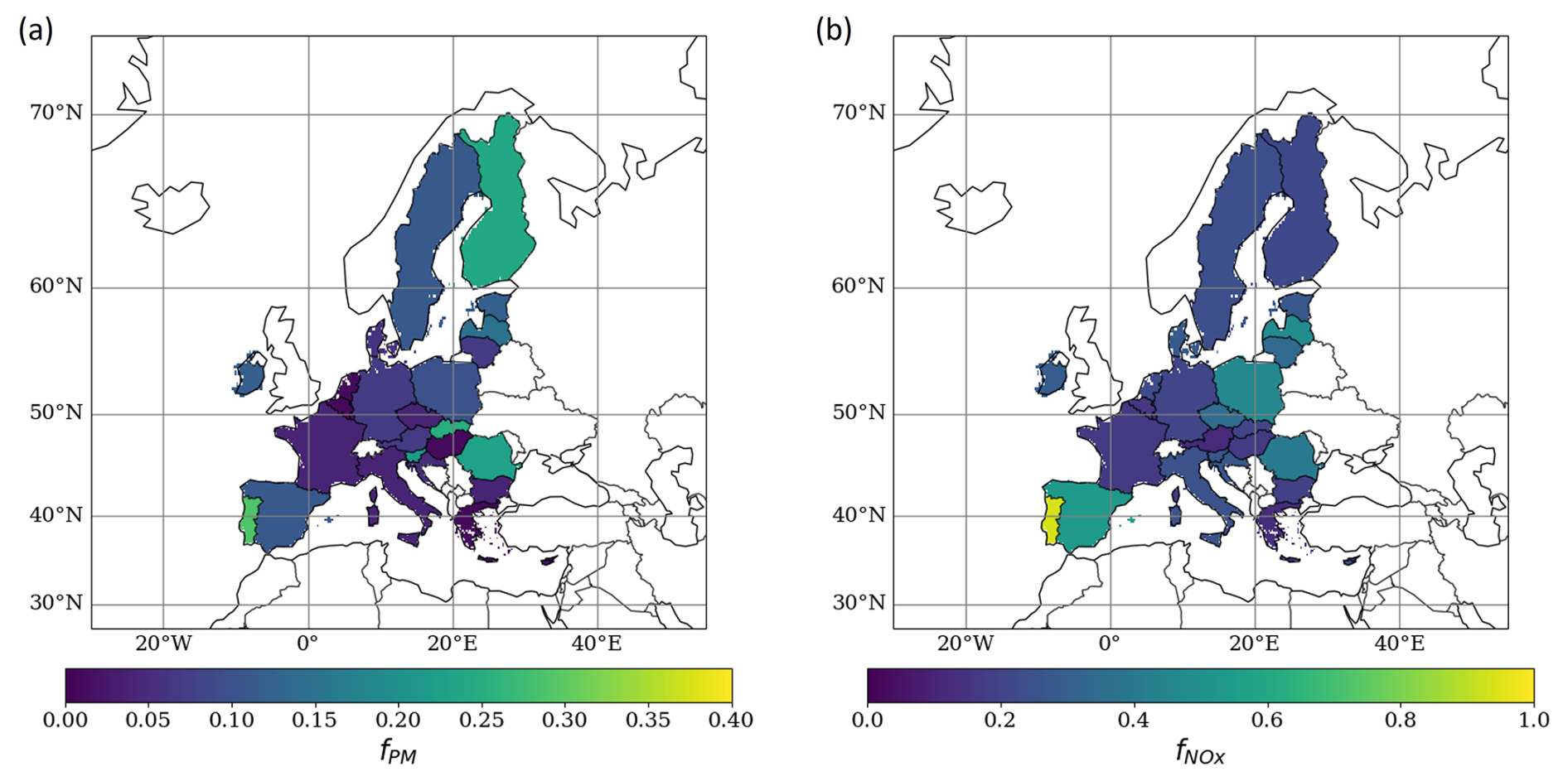
Several energy sources are generally used in European households, and their proportions allocated to space heating are different. As PM and NO_x emissions come from very different energy types, the parameter f(c) can be estimated for the two pollutants (f_PM(c) and $f_{{\mathrm{NO}}_x}\left(c\right)$). PM emissions from residential heating come mainly from the consumption of solid fuels and oil that are used in fireplaces, stoves and oil-fired boilers. Based on the Eurostat dataset, the average fractions of the energy classes “solid fossil fuels, peat products, oil shale and oil sands” (SFF-P1000-S2000 SIEC code) and “primary solid biofuels” (R5110-5150-W6000RI SIEC code) consumed for space heating in relation to all household activities are calculated for each EU 27 country, to derive f_PM(c). The same fraction is calculated for the energy type “natural gas” (G3000 SIEC code) to represent the fraction of NO_x emissions from space heating ($f_{{\mathrm{NO}}_x}\left(c\right)$) that comes mainly from the use of gas boilers. As biogas is mainly used for transport, it is not included. Other pollutants, such as carbon monoxide (CO) and volatile organic compounds (VOCs) for example, are characterized by the reference value (0.2, Guevara et al., 2021b).

Figure 1 presents f_PM(c) and $f_{{\mathrm{NO}}_x}\left(c\right)$ for each EU 27 country. With the exception of a few countries, $f_{{\mathrm{NO}}_x}\left(c\right)$ remains between 0.1 and 0.4. Latvia (0.48), Poland (0.47), Romania (0.41) and Spain (0.54) use more than 40 % of natural gas for household activities other than heating (e.g. water heating, cooking). Portugal stands out from the other countries, with a high $f_{{\mathrm{NO}}_x}\left(c\right)$ value (0.94). Portugal uses very little gas in its energy mix for domestic activities (9 % compared to 32 % for the EU 27 average), and this small fraction is mainly used for heating water (62 % compared to 19 % for the EU 27) and for cooking (35 % compared to 6 % for the EU 27). For most countries, f_PM(c) is less than 0.10. It is even equal to 0.01 for Belgium, Greece, Hungary, Malta and the Netherlands, which means that almost all solid fossil fuels are used exclusively for heating. With Portugal (0.29), Slovakia (0.25) and Finland (0.24) the highest, f_PM(c) does not exceed 0.30 in the EU 27 countries.

Figure 1 Parameters f_PM(c) (a) and $f_{{\mathrm{NO}}_x}\left(c\right)$ (b) based on Eurostat (2023). The list of numerical values per country can be found in Table S1 in the Supplement. For countries without data to compute f(c), the available European average is assigned (i.e. 0.25 for $f_{{\mathrm{NO}}_x}\left(c\right)$ and 0.09 for f_PM(c)).

2.2.2 The temperature threshold (Tb(c))

Tb(c) is calculated by fitting it to the national domestic gas consumption statistics used as a proxy of heating use (hereafter referred to as Tb_fit(c)) taken from the Transparency Platform provided by the European Network of Transmission System Operators for Gas (ENTSOG, 2023). In this article, Tb_fit(c) is compared with the reference threshold of 15.5 °C, which does not vary by country (hereafter referred to as Tb_ref.).

The Transparency Platform is a web tool that provides technical and commercial data on gas transmission systems for several countries. Measurements of physical gas flow at a daily frequency are available at interconnection points and connections to different types of infrastructure: liquefied natural gas terminals, production facilities, storage facilities, transmission systems, distribution systems and consumer metering systems. As industrial consumers require large quantities of high-pressure gas for their plants, they are generally directly connected to the pipelines. This ensures that the distribution network (carrying low-pressure gas) is used for domestic purposes (both commercial and residential). For the purposes of this study, only data related to distribution systems and consumer metering systems are retained. In addition, only countries for which the proportion of gas used by households for space heating is at least 60 % are kept, which ensures that daily gas consumption is an appropriate proxy for assessing the temperature threshold. Based on these criteria and available data, data are gathered for eight countries (Hungary, Romania, Italy, France, Belgium, the Netherlands, Latvia and Estonia). These countries cover the different regions of Europe, being as representative as possible of the diversity of weather conditions and building construction. The operator and the temporal coverage of gas flow data for each country can be found in the Supplement (Table S2).

Tb_fit(c) is calculated by fitting the country-averaged TF_HDD(c) (see Eq. 2) to the temporal factor of domestic gas consumption (TF_gas(c); see Eq. 4) by country using an optimization solver by machine learning. Based on non-linear optimization, the Nelder–Mead algorithm (Gao and Han, 2012) provides the minimized RMSE as the successful solution. The daily TF_gas(c,d) for the year n is calculated as follows:

$$\begin{array}{}\text{(4)}& {\mathrm{TF}}_{\mathrm{gas}}(c,d,n)={\displaystyle \frac{Q(c,d,n)}{\stackrel{\mathrm{‾}}{Q(c,n)}}},\end{array}$$

where $\stackrel{\mathrm{‾}}{Q(c,n)}$ is the yearly average of distribution gas flow [kWh d⁻¹] . In order to reduce dependence on daily data for a specific year, which could be not representative of the country's domestic consumption, the fitting was based on data over several years (from 2 to 6 years over the 2016–2021 period depending on the country). TF_HDD(c) is calculated from the daily average temperature, using hourly T2m data from the ERA5 reanalyses (Muñoz-Sabater et al., 2021).

An example with Belgium and Romania is shown in Fig. 2, where TF_gas(c) shows a marked seasonal cycle with a maximum in winter and a minimum in summer. It presents significant day-to-day variations during the winter period. Using the calculated Tb_fit(c) (15.92 and 16.63 °C for Belgium and Romania respectively), TF_HDD(c) manages to closely follow the evolution of TF_gas(c). The peaks of gas consumption, corresponding to colder periods, are reproduced by the HDD parameterization. The time series of TF_gas(c) and TF_HDD(c) (for both Tb_fit(c) and Tb_ref.(c)) for the other six countries are available in Fig. S1 in the Supplement.

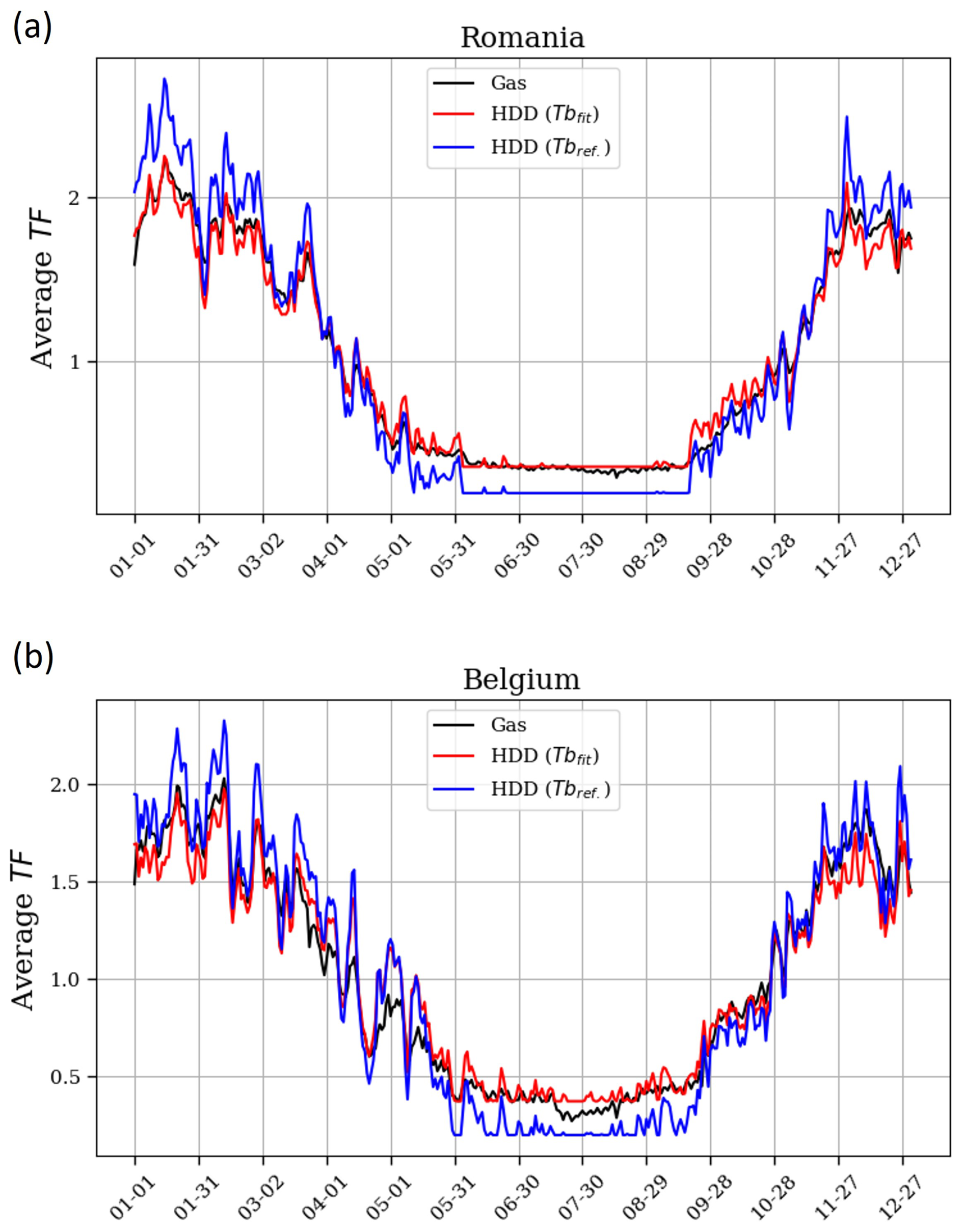
Figure 2 Daily evolution of TF(c) (unitless) for gas consumption (in black), for HDDs with Tb_fit (in red) and for HDDs with Tb_ref. (in blue). TF(c) is illustrated for Romania (a) and for Belgium (b), averaged over the period 2018–2021 and 2016–2021 respectively.

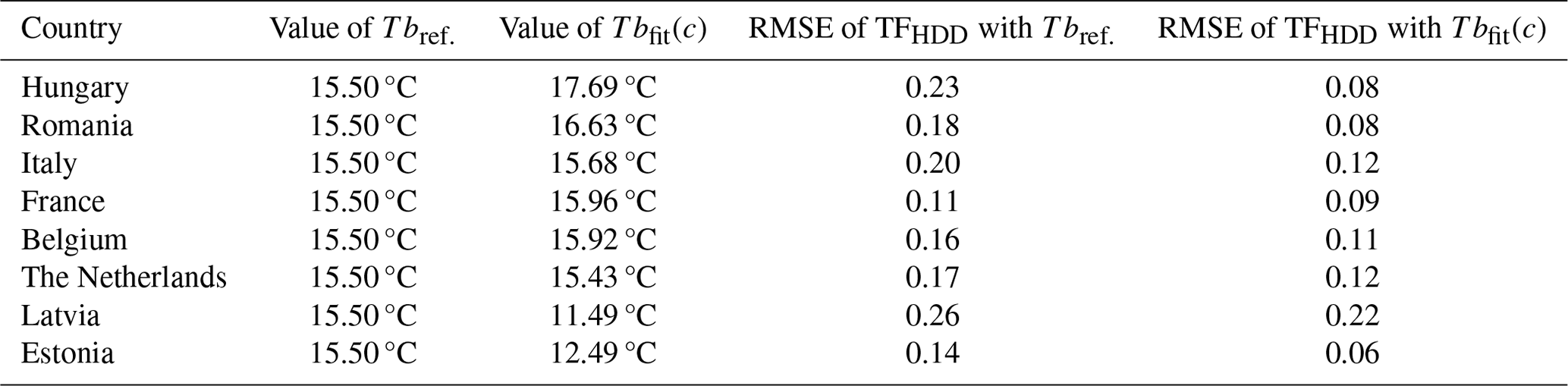
Calculated Tb_fit(c) values by country are shown in Table 1. TF_HDD(c) using Tb_fit(c) and Tb_ref. can be compared. The mean RMSE between TF_gas(c) and TF_HDD(c) is lower by −36 % using Tb_fit(c) compared to Tb_ref. on average over the eight countries. The Tb_fit(c) values found for the eight European countries highlight a latitudinal gradient decreasing from 15.68 °C for Italy to 11.49 °C for Latvia. A lower Tb_fit(c) means that heating in a given country is activated for a lower threshold of ambient temperature. Ciais et al. (2022) obtained a similar south–north gradient (ranging from 16.4 to 13.5 °C) by applying linear regressions between natural gas consumption and temperature data over 2016–2019. Grythe et al. (2019) used observed BaP in situ concentrations, as a proxy of wood burning emissions, at five urban sites in Norway to determine a Tb around 10 °C for Norway rather than the usual value of 15 °C. The Finnish Meteorological Institute applies a Tb value for calculating HDDs that varies according to the season: 10 °C from spring onwards and 12 °C from autumn onwards (StatFin, 2023).

Table 1 Value of Tb_ref. and Tb_fit(c) for each country calculated from the national supplier's gas data using an optimization solver (second and third columns). The fourth and fifth columns compare the average RMSE between TF_gas(c) and TF_HDD(c) using Tb_ref. and Tb_fit(c).

Finally, the European map of Tb_fit is derived by interpolating the values of the 8 fitted countries to the other EU 27 countries using the inverse distance weighting (IDW) (Fig. 3). As Sweden and Finland are not in the interpolated domain, they have been assigned the averaged value of Estonia and Latvia (11.99 °C). The interpolated value is calculated as the distance-weighted average of the central coordinates of the eight neighbouring fitted countries, as follows:

$$\begin{array}{}\text{(5)}& x_p={\displaystyle \frac{{\sum }_{c=\mathrm{1}}^Z\frac{x_c}{d_c}}{{\sum }_{c=\mathrm{1}}^Z\frac{\mathrm{1}}{d_c}}},\end{array}$$

where x_p is the interpolated value, x_c the Tb_fit(c) value of the Z(=8) neighbouring countries c, and d the distance (in km) between the national central coordinates. For countries outside the EU 27, the value assigned is the average Tb_fit of the eight countries, namely 15.16 °C.

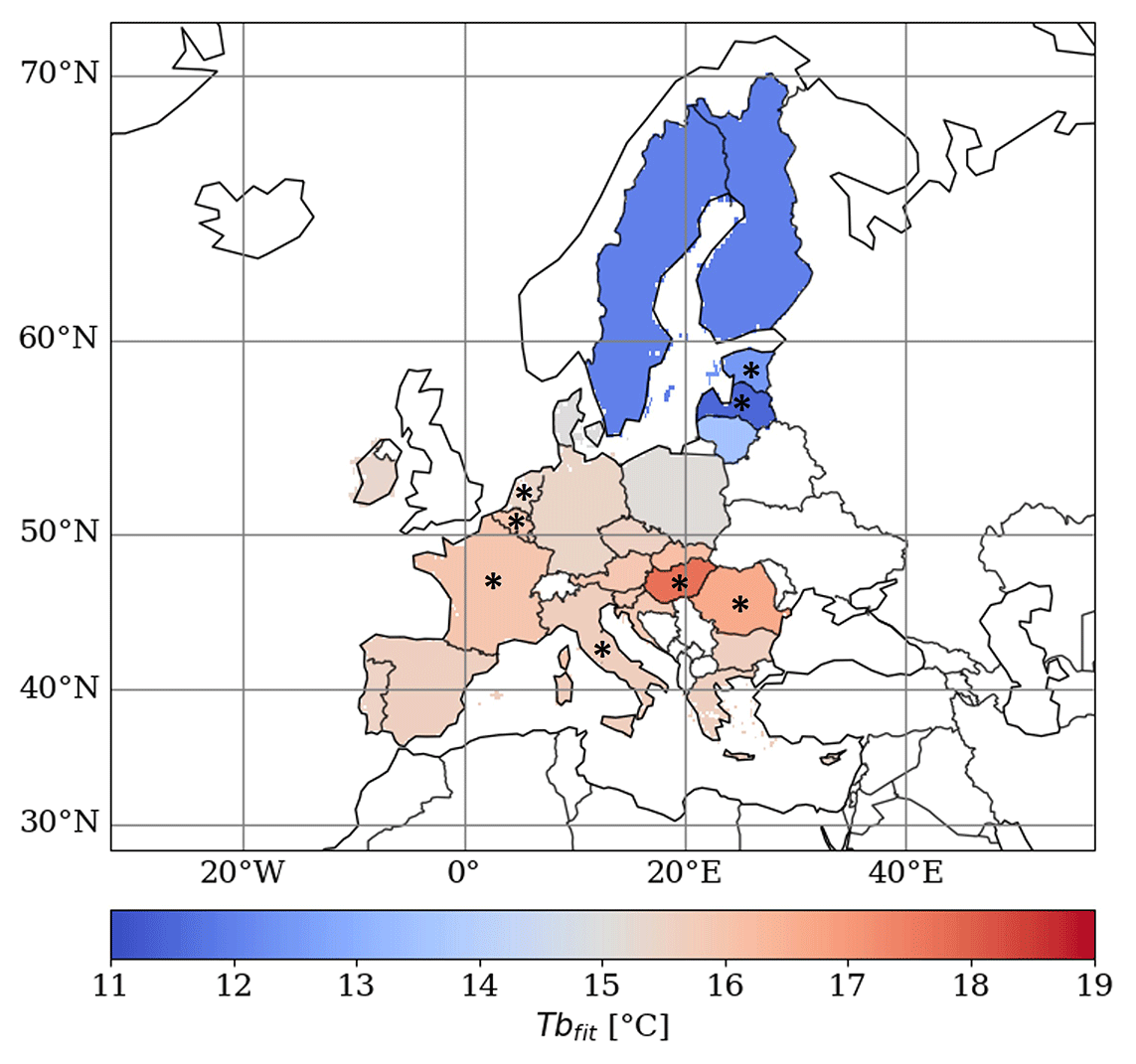
Figure 3 Estimated Tb_fit(c) for EU 27 countries calculated on the basis of domestic gas consumption from the ENTSOG platform. The list of numerical values per country for Tb_fit(c) can be found in the Supplement (Table S1). Countries marked with a star are those for which the Tb_fit(c) has been fitted. The other countries are interpolated using the IDW approach.

3 Setup of the numerical experiments to assess the impact of HDD methodology

3.1 Daily variability of emissions in the residential sector

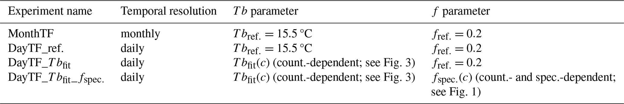
Table 2 shows the different simulation experiments carried out in this work. Different configurations of HDD-based temporal factors are used to distribute anthropogenic emissions from GNFR_C over the year. The different experiments are as follows:

• “MonthTF” distributes emissions temporally with monthly profiles (m) for each grid cell (i, j) for the corresponding year (n), based on the calculation of monthly average HDDs. Therefore, TF$(i,j,m,n)$ is left constant for each month without accounting for day-to-day variation, as possibly found in the literature (e.g. Ebel et al., 1997; Denier van der Gon et al., 2011).

• “DayTF_ref.” is based on HDDs to derive the daily TF${}_{\mathrm{HDD}}(i,j,d,n)$ (see Eq. 2). The reference parameters f_ref. (i.e. 0.2) and Tb_ref. (i.e. 15.5 °C), as described in Guevara et al. (2021b), are used.

• “DayTF_Tb_fit” is the same as DayTF_ref. but uses Tb_fit(c) (country-dependent; see Fig. 3) in the calculation of $TF(i,j,d,n)$.

• “DayTF_Tb_fit_f_spec.” is the same as DayTF_Tb_fit but uses f_spec.(c) (country- and species-dependent; see Fig. 1) in the calculation of T$F(i,j,d,n)$.

Hourly profiles are taken from Guevara et al. (2021b) and are not modified between the different experiments. Hourly profiles vary according to the day of the week, particularly at weekends, and generally peak at 08:00 and 20:00 UTC+0, depending on the species emitted.

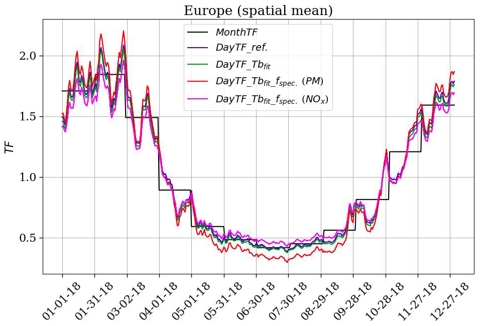
Figure 4 shows the seasonal variation of the daily temporal factors for the different experiments (European average) used to distribute GNFR_C emissions. There are significant variations on both a daily and seasonal scale between the experiments. The DayTF_Tb_fit_f_spec. experiment for PM shows the greatest seasonal variation, reaching a maximum of ∼ 2.2 in winter and a minimum of ∼ 0.2 in summer. The resulting effect of the experiments on the total anthropogenic emissions of fine and coarse particles and NO_x can be found in the Supplement (Fig. S2). Each HDD-based experiment is tested in order to both simulate air quality with the CHIMERE CTM model (see Sect. 4.1) over the year 2018 and calculate multi-year projection of emissions (see Sect. 4.2) over the 2009–2018 period.

Table 2 Characteristics of the experiments conducted to distribute annual anthropogenic emissions from the “other stationary combustion” sector (GNFR_C) over the grid domain i,j.

Figure 4 Daily temporal factor for GNFR_C for the different experiments detailed in Table 2 averaged over Europe for 2018.

3.2 Air quality simulations for the year 2018

3.2.1 Anthropogenic emission datasets

Several sets of emissions data are used to meet the objectives of this work. Firstly, annual gridded totals of anthropogenic emissions are provided by the Regional Inventory for Air Pollutant “CAMS-REG-AP-v5.1” (Kuenen et al., 2022). The national totals by country come from the EMEP Centre on Emission Inventories and Projections (CEIP, 2023), which is responsible at the European level for compiling the emissions of the State Parties to the “Convention on long-range transboundary air pollution” (LRTAP) for official publication. The annual emission totals reported for a given year are recalculated each subsequent year in accordance with any updated guidelines and/or datasets.

Based on specific spatial proxies for the distribution of emissions, “CAMS-REG-AP-v5.1” covers the European domain at a 0.05°×0.10° grid resolution. Specifically designed for air quality modellers, it provides emission for the main pollutants (NO_x, SO₂, non-methane VOCs (NMVOCs), NH₃, CO, PM₁₀, PM_2.5 and CH₄) at a wide range of sector levels. Following Denier Van Der Gon et al. (2015), condensable PM is represented in this inventory in a consistent way for all European countries. In addition to emissions from stationary residential combustion, the “other stationary combustion” sector (GNFR_C) also includes stationary commercial combustion (which can be assumed to behave in the same way as the residential sector) and stationary combustion from agriculture, forestry and fishing, which may not behave in the same way but whose contribution to the total GNFR_C is negligible. Emissions from power stations and other industries are not covered by sector C but by GNFR_A and B respectively. The annual average spatialized contribution of sector C to total anthropogenic emissions of NO_x and PM over the period 2009–2018 (based on CAMS-REG-AP-v5.1) can be found in the Supplement (Fig. S3). On average over EU 27 countries (national totals from CEIP, 2023), the contribution of GNFR_C is 9.1 % for NO_x, 33.4 % for PM₁₀ and 51.6 % for PM_2.5. Emissions of PM are split into primary organic aerosol (POA), elemental carbon (EC) and other primary PM based on the CAMS speciation table.

Temporal profiles for other sectors than GNFR_C are taken from the “CAMS-TEMPOv3.2” product (Guevara et al., 2021b) that provides temporal profiles of European emissions of the main atmospheric pollutants. Those gridded temporal factors are available for monthly, daily, weekly and hourly cycles. Identifying the main emission drivers for each sector, the profiles are calculated on the basis of statistical information linked to the variability of the emissions (e.g. traffic counts) and parameters dependent on meteorology.

3.2.2 The CHIMERE configuration

The CHIMERE v2020r1 model (Menut et al., 2021), a regional three-dimensional Eulerian CTM, is used to simulate air quality over the year 2018 by testing different HDD parameterizations. CHIMERE represents the processes of gas-phase chemistry, aerosol formation, atmospheric transport and deposition. The chemical scheme used is MELCHIOR2 (Derognat, 2003), which includes 44 species and around 120 reactions. Aerosol microphysics and thermodynamics as well as secondary aerosol formation mechanisms are represented in the inorganic and organic aerosol module from Couvidat et al. (2012, 2018). POAs are assumed to be semivolatile and can partition between the gas and particle phase as a function of temperature and the concentration of organic aerosols. The gas-phase fraction can react with the hydroxyl radical and form lower-volatility compounds via ageing. Secondary organic aerosols (SOAs) are formed with the hydrophilic/hydrophobic organic (H²O) mechanism. The Fast-Jx module version 7.0b (Bian and Prather, 2002) calculates the photolysis rates accounting for the radiative impacts of aerosols online. Vertical advection and horizontal advection follow the scheme of Van Leer (1977). The physical and chemical time steps are 10 min. The simulated domain covers Europe, with the following coordinates as corners: 30–72° N, 25–45° E. The spatial resolution is 0.2°×0.2° (around 20 km). Nine vertical layers from 998 up to 500 hPa are used. The meteorological fields are from the operational analysis of the Integrated Forecasting System (IFS) model of the European Centre for Medium-Range Weather Forecasts (ECMWF). Time-varying boundary conditions for gas and dust aerosols are also provided by the IFS (Flemming et al., 2015; Rémy et al., 2022).

Natural emissions are calculated online: biogenic emissions using the MEGAN model (Guenther et al., 2006, 2012), sea salt and dimethyl sulfide marine emissions following the scheme of Mårtensson et al. (2003) and Liss and Mervilat (1986) respectively, and finally mineral dust emissions based on the parameterization of Marticorena and Bergametti (1995) and Alfaro and Gomes (2001). Emissions from forest fires are not included.

3.2.3 In situ observations for validation

In situ measurements of surface concentration are used to evaluate air quality simulations based on the CHIMERE model. These observations are taken from the European air quality observation database AQ e-Reporting (EEA, 2023), which gathers air quality data provided by EU members states and other EEA collaborating countries.

The analyses presented in this work focus mainly on NO₂, PM₁₀ and PM_2.5 species. The stations selected are background stations (urban, suburban and rural type). For the calculation of daily averages and maximums, stations that do not cover an availability ratio of at least 75 % of hourly measurements are excluded. Over the whole domain, our study considers 1831 stations for NO₂, 1070 for PM₁₀ and 540 for PM_2.5 for the year 2018.

3.3 Modelling annual emissions between 2009 and 2018

3.3.1 Formula

Total annual emissions from GNFR_C can be projected over several years by calculating HDDs. While emission inventories take at least 2 years to be officially published, temperature reanalyses are available in a much shorter time frame (from a few weeks to a few months). By assuming that changes in emissions from residential and commercial heating are dominated by the effect of the meteorology (rather than changes in emission factors and changes in heating habits), projected emissions (E_proj(i,j)) can be calculated using the total gridded emissions E(i,j) of the reference year n_ref and comparing HDD factors between the projected year n_ref+x and the reference year n_ref (Eq. 6).

$$\begin{array}{}\text{(6)}& \begin{array}{rl}{E}_{\mathrm{proj}}& (i,j,n_{\mathrm{ref}+x})=E(i,j,n_{\mathrm{ref}})\\ & \times \left({\displaystyle \frac{\mathrm{1}}{N}}\times f+{\displaystyle \frac{{\sum }_{d=\mathrm{1}}^N\mathrm{HDD}(i,j,d,n_{\mathrm{ref}+x})}{{\sum }_{d=\mathrm{1}}^N\mathrm{HDD}(i,j,d,n_{\mathrm{ref}})}}\times (\mathrm{1}-f)\right)\end{array}\end{array}$$

Gridded emission totals from the CAMS-REG-AP-v5.1 inventory (Kuenen et al., 2022) are used to model emissions of PM_2.5, PM₁₀ and NO_x from GNFR_C between 2009 and 2018. The multi-year projections using the HDD method are calculated for x=2 (equivalent to the delay in the official publication of emissions) and for x=3 (to assess the feasibility of the method in a longer publication scenario). They are compared with persistence (also for x=2 and x=3), which assumes that emissions in subsequent years are identical to those in the reference year.

3.3.2 Estimated uncertainty of nationally reported emissions

In the process of emission reporting of the LRTAP Convention, countries have to update emissions for several recent years when they introduce a change in the emission calculation methodology. Therefore, to assess if the uncertainties introduced in the modelling of emission with HDDs are comparable to emissions uncertainties, we compare those different reporting years for the same target year. As suggested in the Informative Inventory Report from CEIP/EMEP (Schindlbacher et al., 2021), the magnitude of the recalculation can provide a general estimate of the uncertainty of released emissions. This uncertainty (U_+z), expressed as a percentage, is calculated based on the average relative difference between total national emissions (E(c)) of the year (n) reported for a given year (yr) and the total for the same year but reported in subsequent years (z) up to 2 years (U₊₂ with $z=\mathit{\{}\mathrm{1},\mathrm{2}\mathit{\}}$) and 3 years (U₊₃ with $z=\mathit{\{}\mathrm{1},\mathrm{2},\mathrm{3}\mathit{\}}$), as follows:

$$\begin{array}{}\text{(7)}& U_{+z}(c,n)={\displaystyle \frac{E_{\mathrm{yr}+z}(c,n)-E_{\mathrm{yr}}(c,n)}{E_{\mathrm{yr}}(c,n)}}\times \mathrm{100}.\end{array}$$

$U_{+\mathrm{2}}(c,n)$ and $U_{+\mathrm{3}}(c,n)$ are calculated in this work for the official publication of national emissions totals for each year n between 2009 and 2018 and then averaged over this period. Finally, the national totals of EU 27 countries in GNFR_C supplied by CEIP are used. This method enables uncertainty to be calculated quickly for a specific sector and by country.

4 Results

4.1 Impact on air quality modelling skills

4.1.1 Overview of the year 2018

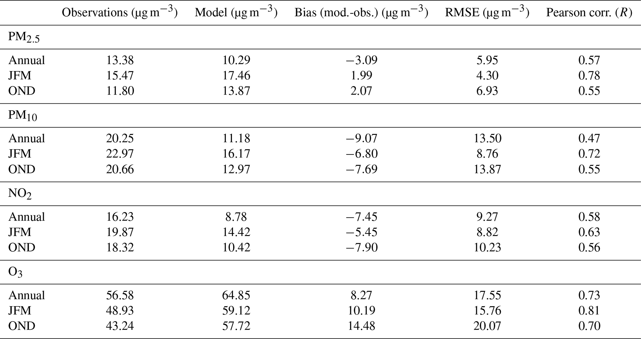
In order to provide a general validation of the baseline simulation, surface concentrations simulated with the MonthTF experiment are compared with AQ e-Reporting observations over the whole of 2018, with a focus on winter (defined here from January to March) and autumn (from October to December). Table 3 shows the scores on daily concentrations averaged over all the European background stations. On average, annually, the bias (model minus observations) is negative for PM_2.5 (−3.09 µg m⁻³), PM₁₀ (−9.07 µg m⁻³) and NO₂ (−7.45 µg m⁻³) and positive for O₃ (+8.27 µg m⁻³). In winter, the bias for PM_2.5 becomes positive (+1.99 µg m⁻³). The RMSE calculated over winter is lower (e.g. 4.30 µg m⁻³ for PM_2.5) than over the whole year (5.95 µg m⁻³ for PM_2.5) for each species analysed. The correlation coefficient R on annual average is almost equal to or greater than 0.5 for all species (between 0.47 and 0.73). It increases considerably when calculated for winter, between 0.63 and 0.81.

It should also be pointed out that these mean values show considerable spatial and temporal variability. The temporal distribution of the daily bias (see Fig. S4) and the spatial distribution of the stations with their corresponding annual bias (see Fig. S5) are presented in the Supplement. The majority of background stations included in the validation calculation are of the urban or suburban type (between 69 % and 77 % depending on the species). A representativeness bias may lead to a reduction in PM and NO₂ peaks at station points when the regional CTM simulates average concentrations over 20 km grids. Nevertheless, these scores show an overall agreement with those presented in the latest articles using the 2020 version of CHIMERE (e.g. Menut et al., 2021; Guion et al., 2023), as well as with other regional CTMs (e.g. Bessagnet et al., 2016).

Table 3 Validation scores for the CHIMERE reference simulation (MonthTF) calculated from AQ e-Reporting observations for PM_2.5, PM₁₀, NO₂ and O₃ species, averaged over Europe in 2018.

The effect of the different HDD parameterizations integrated in the emissions used in CHIMERE is analysed by comparing the Spearman correlation and RMSE scores in concentration with the available observations (stations averaged by country) for each experiment and more specifically for each country for which the Tb parameter has been calculated based on the national gas data. Using an HDD-based temporal profile, therefore with daily variation by comparison to the baseline simulation MonthTF experiment, mainly affects the simulated concentrations of PM_2.5, PM₁₀ and NO₂ from January to March and from October to December (see Fig. S4). As a result, the spring and summer seasons, when wood heating is almost non-existent in both southern and northern Europe, are not included in the analysis here. The case of the beginning of 2018, characterized by negative temperature anomalies (corresponding to cold spells occurring on a European scale) and high residential heating emissions, will be detailed in Sect. 4.1.2, “Threshold level exceedance during the cold spells at the beginning of 2018”, with a specific analysis on peak concentrations. Figure 5 shows the performance metrics for PM_2.5. There are no observations available from AQ e-Reporting for this pollutant in 2018 for Hungary, Romania, Estonia and Latvia. Analysed individually by country, performance between experiments can vary significantly. For Italy, France, Belgium and the Netherlands in winter, the DayTF_Tb_fit_f_spec. experiment presents the best temporal correlation, with an increase of the Spearman coefficient by +8.7 %, +7.9 %, +10.5 % and +8.6 % compared to the MonthTF experiment. In terms of RMSE scores, DayTF_Tb_fit_f_spec. remains close to the MonthTF experiment, although there is a slight decrease for France and the Netherlands in winter (−0.5 and −1.3 µg m⁻³ respectively). The DayTF_Tb_fit experiment leads to a significant decrease in the RMSE for Belgium and the Netherlands (−1.6 and −3.0 µg m⁻³ compared to MonthTF respectively), which can be explained by a lower overestimation of the modelled concentration peaks in these countries. Indeed, the f_PM parameter is lower in DayTF_Tb_fit_f_spec. (0.01 for Belgium and the Netherlands) than f_ref. (0.20). As the simulations show a positive bias for these two countries (already the case with MonthTF; see Fig. S5), the RMSE scores are higher for DayTF_Tb_fit_f_spec. than for DayTF_Tb_fit. The validation scores obtained also depend on the accuracy of the values provided by the Eurostat dataset. The bias scores can be found in the Supplement (see Fig. S11).

For the autumn season, the HDD parameterization does not appear to have any beneficial effect on performance scores. While the correlation varies very little (about −0.03 for R compared to MonthTF), the RMSE increases, whatever the parameterization (+2.9 µg m⁻³ on average over the four countries compared to MonthTF). However, autumn 2018 does not appear to be the most relevant period for assessing the impact of HDDs, as it was relatively warmer than the average, with no major European cold spell (see Fig. S12).

Performance scores can vary considerably from one country to another (and even more so than between experiments, which, as a reminder, only differ in the parameters of the temporal distribution of heating emissions). This is discussed in more detail in the “Discussion and conclusions” section (see Sect. 5), but national differences in the calculation of emissions and the representation of certain processes such as long-distance transport have an impact on the simulation scores for each country.

The equivalent figure for PM₁₀ can be found in the Supplement (see Fig. S10), with results similar to those for PM_2.5.

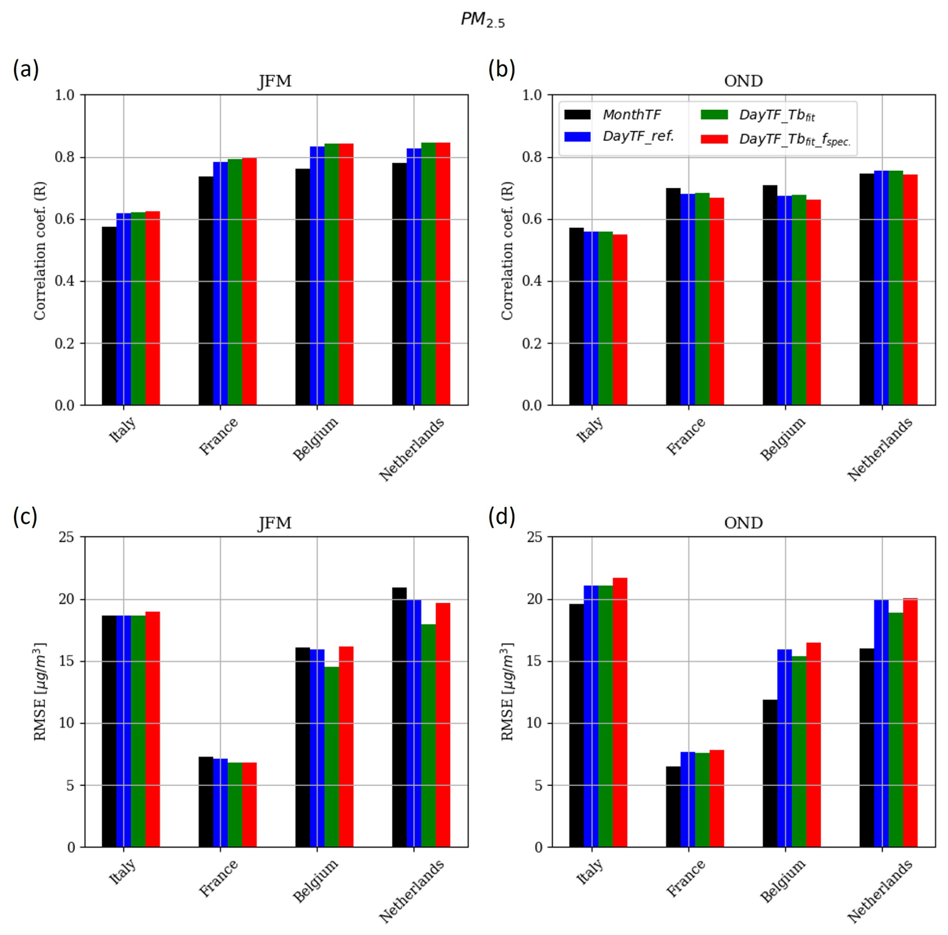
Figure 5 Spearman correlation (R coefficient) and RMSE (µg m⁻³) of hourly PM_2.5 concentrations for the months JFM (panel a and c respectively) and OND (panel b and d respectively), averaged over stations in countries that have been fitted with gas consumption data and for which concentration measurements are available.

The spatial distribution of score variations induced by the DayTF_Tb_fit_f_spec. experiment (shown in Fig. 6 for PM_2.5 in JFM) allows us to identify the regions most sensitive to the adjusted HDD parameters. The Spearman temporal correlation is considerably better (compared to MonthTF), relatively uniformly between and within countries (up to +0.2), with the exception of Belgium, the southern Netherlands and western Poland, where the increase in the R coefficient is smaller (about +0.05). This analysis also shows that the improvement in scores also concerns countries for which the Tb_fit has been interpolated. Being larger in eastern Europe (about −2 µg m⁻³), the decrease in RMSE with experience DayTF_Tb_fit_f_spec. does not concern all countries. The change in RMSE is almost zero in Belgium, the Netherlands, southwestern Germany, eastern Poland and Portugal. The spatial variations in scores for PM₁₀ are similar to those for PM_2.5, while they are very small for NO₂ (as discussed below).

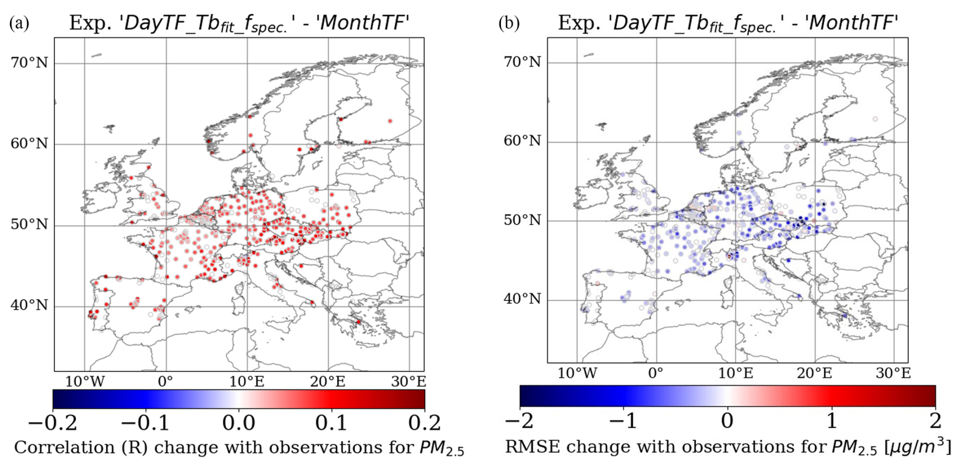
Figure 6 Average change in Spearman correlation (R coefficient) and RMSE (µg m⁻³) (a and b respectively) at stations between the experiment DayTF_Tb_fit_f_spec. and MonthTF simulated in JFM for PM_2.5.

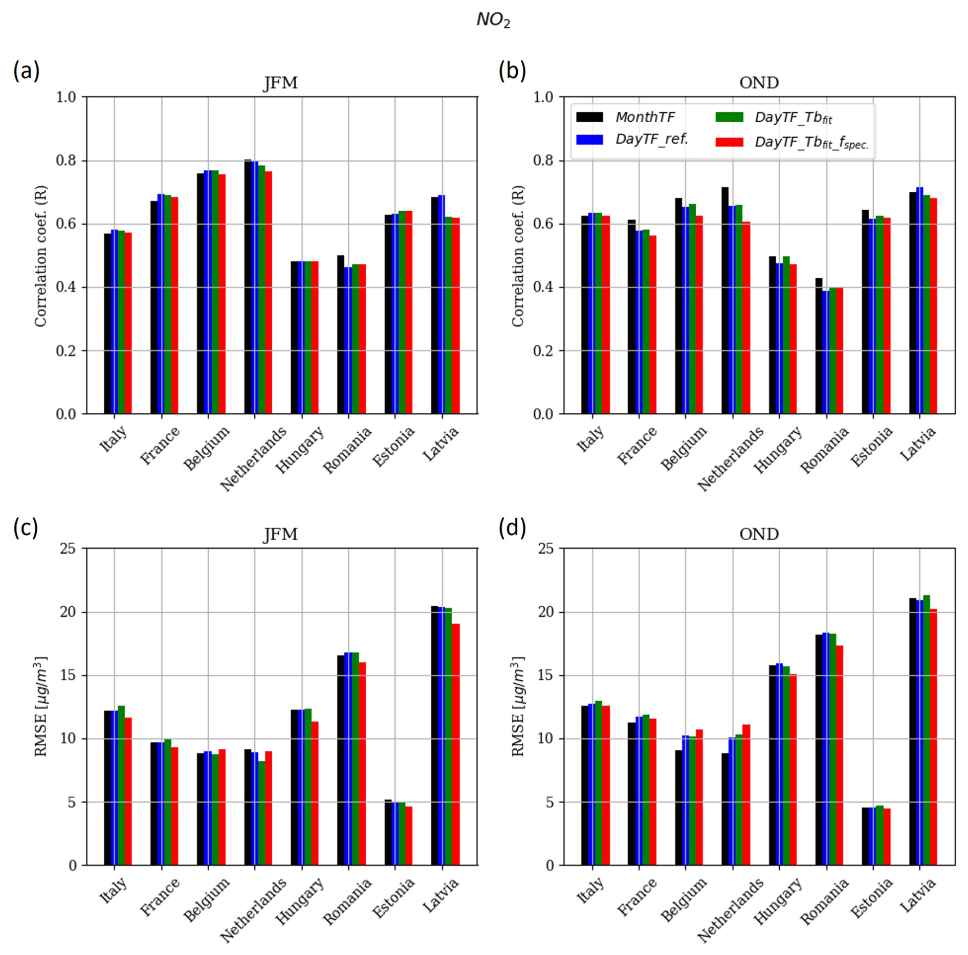
Figure 7 shows the performance metrics for NO₂. With the exception of the Netherlands, Romania and Latvia, the correlation coefficient in winter varies slightly between the CHIMERE experiments. However, DayTF_Tb_fit_f_spec. has the lowest RMSE in winter for Italy, France, Hungary, Romania, Estonia and Latvia, with an average decrease of −4.4 % compared to MonthTF. For the autumn season, HDD-based experiments do not improve the correlation coefficient (for all parameterizations tested), but the RMSE decreases by −3.6 % on average for Hungary, Romania, Estonia and Latvia for DayTF_Tb_fit_f_spec. compared to MonthTF.

Figure 7 Same as Fig. 5 for the NO₂ species.

4.1.2 Threshold level exceedance during the cold spells at the beginning of 2018

February and March 2018 were considerably colder than seasonal normals (up to −4 °C on average across Europe). Several periods of intense cold have been identified and documented by the Copernicus Climate Change Service (C3S) (see Figs. S12 and S13). Three cold spells were reported to have affected most of the European region: from 7 to 10 February, from 26 February to 4 March and from 18 to 27 March. These periods are particularly relevant for analysing the use of HDDs when residential heating increases considerably and therefore for assessing the model capabilities to capture threshold exceedance (e.g. Chen et al., 2017).

Figure 8 shows the temporal evolution of simulated concentrations of PM_2.5, PM₁₀ and NO₂ during JFM, averaged over Europe. The example of France is also shown, with an adjusted identification of cold periods throughout the country from Météo-France (MF, 2019). Time series for other countries can be found in the Supplement (see Figs. S7, S8 and S9). The simulation without HDDs (MonthTF) fails to correctly reproduce the variability driven by cold spells and relatively warmer winter periods, especially from February to March. Compared to PM_2.5 and PM₁₀ observations averaged over Europe, the MonthTF simulation completely misses the concentration peaks of 3 March (underestimation of around 20 µg m⁻³) and, in the case of PM_2.5, overestimates concentrations over the periods 15–20 February and 7–17 March (by +2 to +5 µg m⁻³).

The various peak concentrations of PM_2.5 and PM₁₀ observed during cold periods were relatively well simulated by the HDD-based simulations. The different parameterizations can lead to differences of several µg m⁻³ during PM peaks. The DayTF_Tb_fit_f_spec. simulation is the experiment that best reproduces the PM peaks during periods of intense cold at the European scale, with the exception of the last PM_2.5 peak around 25 March, when concentrations were slightly overestimated (up to 2 µg m⁻³).

For NO₂ species, concentrations between HDD-based experiments can vary slightly (up to 2 µg m⁻³) and more widely compared with MonthTF (up to 6 µg m⁻³). Compared to the European observations, all experiments tend to underestimate daily concentrations by −5 to −10 µg m⁻³. This does not apply to all countries, such as Estonia, Belgium and the Netherlands (see Figs. S7 and S9). Except for the peak on 8 February which was well modelled, NO₂ peaks are less well represented than PM. However, NO₂ peaks do not always correspond to cold periods. It should be pointed out that observations of NO₂ concentration levels during cold spells are not significantly higher than during other periods. This suggests that background NO₂ concentrations are less sensitive to abrupt variations in emissions linked to residential heating, such as during cold weather events. The recent literature (e.g. Grange et al., 2019; Wærsted et al., 2022) highlights a possible significant sensitivity of NO₂ concentrations to changes in road transport emissions linked to temperature changes.

The same analysis was carried out with the maximum daily concentration (see Fig. S6), and the findings are similar. To complete this spatially averaged analysis of JFM 2018, a specific study of threshold exceedance calculated at each measurement station is presented below, detailing the differences in performance in simulating high concentrations between HDD configurations.

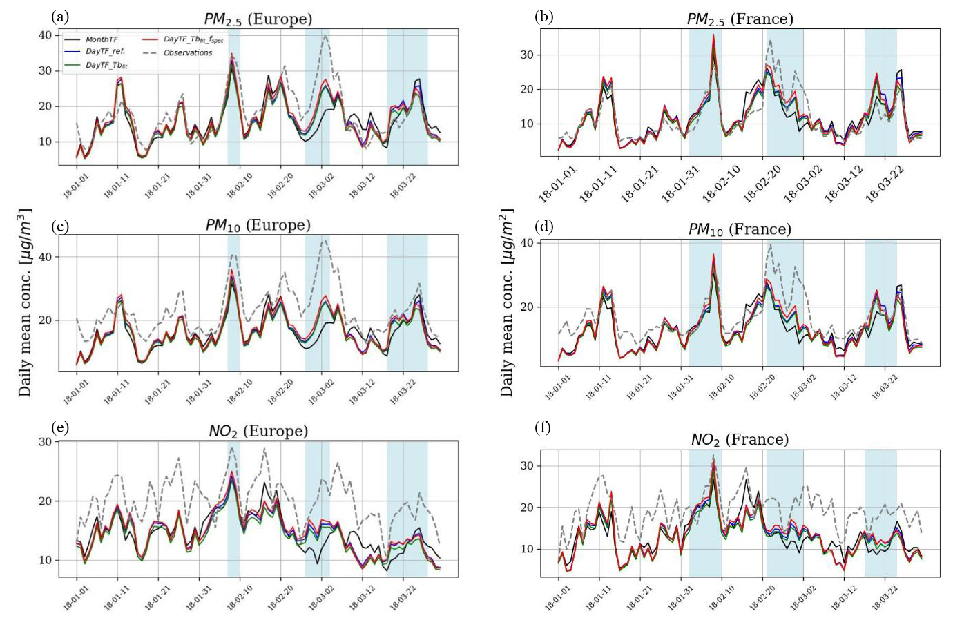
Figure 8 Average daily concentrations [µg m⁻³] of PM_2.5, PM₁₀ and NO₂ in Europe (a, c, e) and in France (b, d, f) between January and March from observations (AQ e-Reporting) and different CHIMERE simulations. The blue areas indicate periods of intense cold as signalled by the C3S and MF for Europe and France respectively.

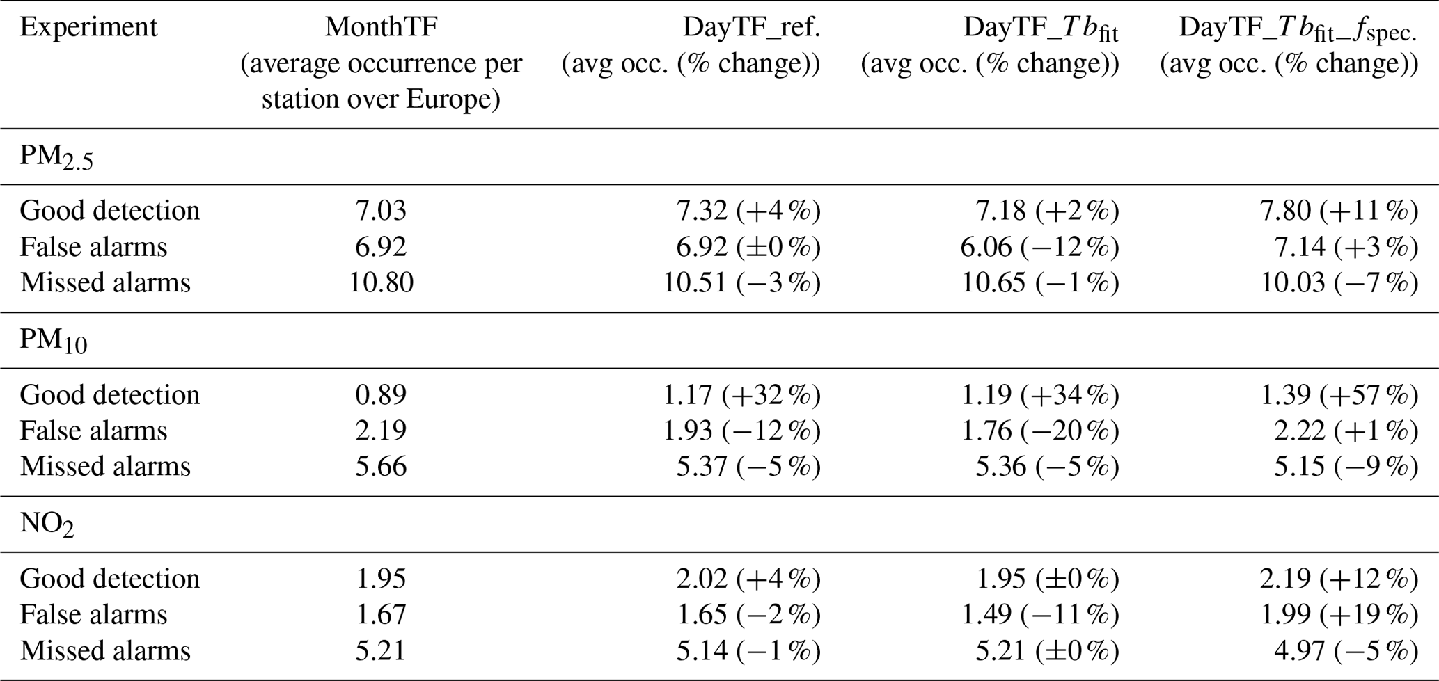
The numbers of exceedance of daily concentration thresholds of 25 µg m⁻³ for PM_2.5, 50 µg m⁻³ for PM₁₀ and 40 µg m⁻³ for NO₂ (based on the Directive 2008/50/EC of the European Parliament and of the Council on ambient air quality and cleaner air for Europe) have been calculated at each monitoring station over Europe for JFM months of 2018. Table 4 shows the average number (per station) of good detection, false alarms and missed alarms, in regards to the observed concentrations.

Compared to the MonthTF experiment, the number of good detection increases and the number of missed alarm decreases when HDDs are included, for all combinations of parameters for the species PM_2.5 (+6 % on average for good detection and −4 % for missed alarms), PM₁₀ (+41 % and −7 %) and NO₂ (+6 % and −2 %). The countries most concerned by these changes, according to the network of measuring stations available, are Belgium, the Netherlands, Poland and Slovakia. The number of false alarms decreases with DayTF_ref. (−12 % for PM₁₀ and −2 % for NO₂) and DayTF_Tb_fit (−12 % for PM_2.5, −20 % for PM_2.5 and −11 % for NO₂) and increases with DayTF_Tb_fit_f_spec. (+3 % for PM_2.5, +1 % for PM_2.5 and +19 % for NO₂). However, this percentage increase in false alarms for DayTF_Tb_fit_f_spec. remains lower than its increase in good detection for PM_2.5 and PM₁₀.

Among the different HDD configurations, the experiment DayTF_Tb_fit_f_spec. has the largest increase of good detection (+11 % for PM_2.5, +57 % for PM₁₀ and −15 % for NO₂) and the largest decrease of missed alarms (−7 % for PM_2.5, −9 % for PM₁₀ and −5 % for NO₂). Finally, DayTF_Tb_fit_f_spec. presents the best probability of detection for PM_2.5 (0.45), PM₁₀ (0.21) and NO₂ (0.31), as illustrated on the performance diagrams (designed by Roebber, 2009) in the Supplement (see Fig. S14).

Table 4 Average number per station (over Europe) of good detection, false alarms and missed alarms simulated by CHIMERE for the MonthTF experiment and variation (in %) with the other HDD-based experiments for JFM. Based on Directive 2008/50/EC, the threshold values for average daily concentrations not to be exceeded were set at 25 µg m⁻³ for PM_2.5, 50 µg m⁻³ for PM₁₀ and 40 µg m⁻³ for NO₂.

4.2 Multi-year emission projections

Based on temperature, HDDs can be used to project emissions from the GNFR_C sector for a given year as an annual total (see Eq. 6) but also in near-real time on a daily time step (by normalizing the HDDs of the current day with the daily average HDDs of the base year). The use of HDDs to simulate the day-to-day variability of residential emissions does not carry a specific risk in the context of simulations for a past year (reanalyses), as the annual heat sum of the corresponding year is known and can be used to normalized total emissions. Conversely, when used in a forecast setup, using HDDs can induce a deviation from the input emissions, as the heat sum of the running year is unknown. This deviation is legitimate as in a colder (milder) than expected winter, emissions should rightfully be larger (lower) than originally prescribed. There is no reason that using emission from a past year (such an approach, referred to as persistence, is routinely used for the operational forecast) would be more legitimate. It is however important to document that risk of deviation. This second part is therefore devoted to the use of HDDs to estimate the total annual emissions of the GNFR_C sector.

In this section we compare the annual total emission modelled with HDDs to the uncertainty related to emission reporting mechanism (see Sect. 3.3.2), and we also compare the deviation when using a persistence approach. Because of the spatialization of the Tb_fit(c) and f(c) parameters and the best modelling results in terms of concentration peaks and threshold exceedance, the HDD-based experiment DayTF_Tb_fit_f_spec. is used in this section. As the analyses results on PM_2.5 emissions are very similar to those for PM₁₀, the results in this section will only be presented for PM_2.5 and NO_x emissions.

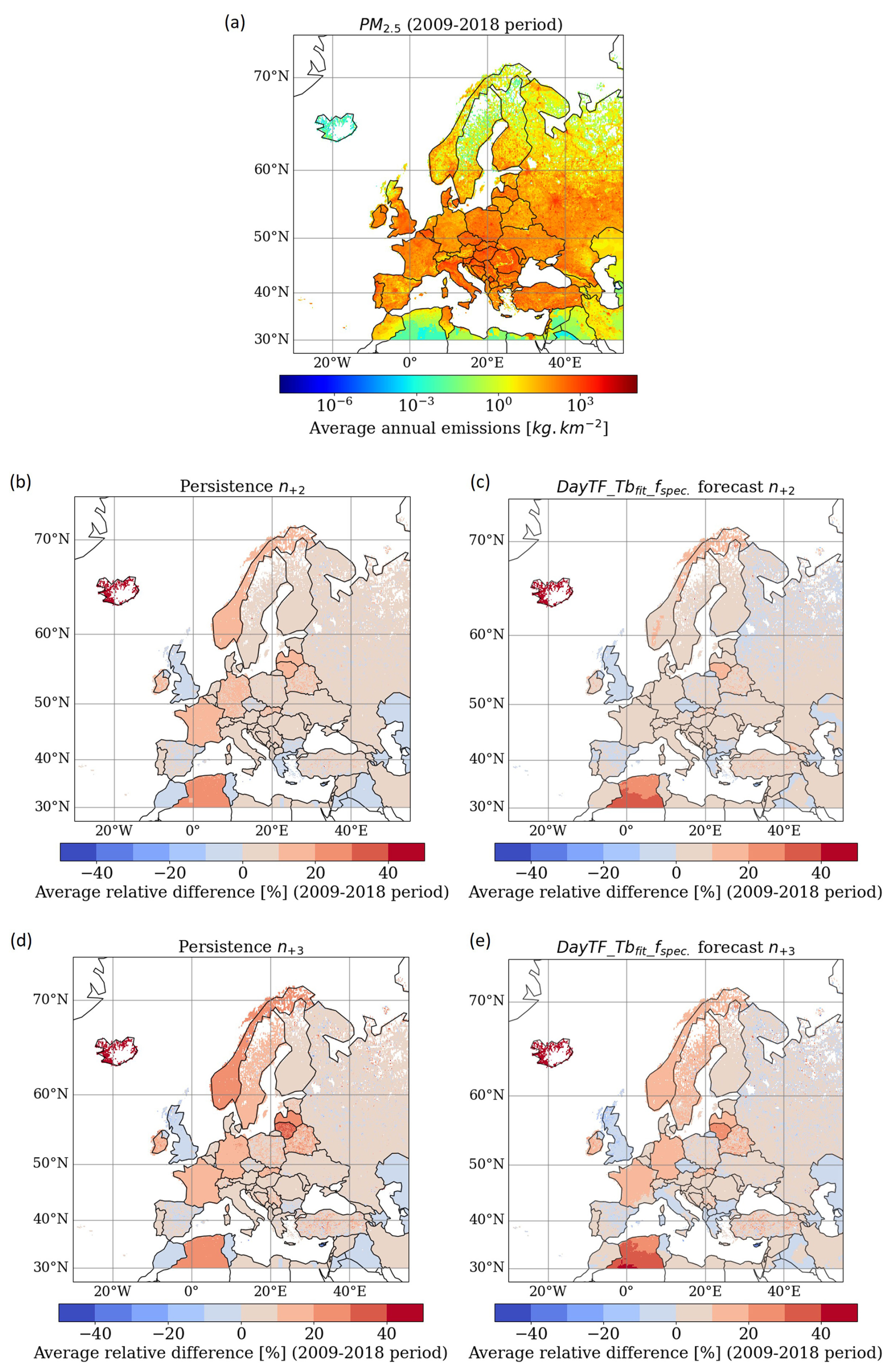
Figure 9 Spatial distribution of average annual PM_2.5 emissions [kg km⁻²] from GNFR_C (2009–2018 period), based on the CAMS-REG-AP-v5.1 inventory (a). Average relative difference using DayTF_Tb_fit_f_spec. to project in n₊₂ (b) and in n₊₃ (d) each year between 2009 and 2019, compared to the reported emissions. Average relative difference using the persistence method for n₊₂ (c) and n₊₃ (e) over 2009–2018.

Figure 9 shows the average reported emissions of PM_2.5 and the average relative difference using DayTF_Tb_fit_f_spec. and the persistence for projected years n₊₂ and n₊₃ (over the 2009–2018 period). The same figure for NO_x emissions is available in the Supplement (see Fig. S15). On a European scale (grid average) for PM_2.5 (NO_x) emissions, the relative difference in n₊₂ is 4.2 % (5.0 %) for the HDD-based projections and 4.6 % (5.3 %) for the persistence. The deviation from reported emissions varies spatially, depending on the country, both for HDD-based projections and for persistence. For France, Germany, Norway, Ireland and Latvia, the HDD method leads to significantly smaller differences with the reported PM_2.5 emissions (by about −10 %) than the persistence method.

As expected a higher deviation is obtained for n₊₃ than for n₊₂ (with both the HDD and persistence approach) at the European level, but the HDD method again shows a lower average deviation (5.2 % for PM_2.5 and 6.7 % for NO_x) than persistence (6.2 % for PM_2.5 and 7.8 % for NO_x). Norway, Latvia and Lithuania benefited from a considerable reduction of relative difference with the HDD method for PM_2.5 emissions (by about −10 %). Algeria shows a larger relative difference (compared to the persistence), but its total emissions remain low compared with other European countries. Finally, an interesting feature of the HDD method is that it can provide more detailed spatial information within the same country (e.g. southeastern France, northern Italy), since HDDs depend on gridded temperature fields.

The average relative deviations induced by the DayTF_Tb_fit_f_spec. projection and the persistence method are compared to the reporting uncertainty estimated from the variability of emission reporting (see Sect. 3.3.2) for each EU 27 country. An example is given with France in Fig. 10 over the 2016–2018 period. Compared with 2016, 2017 and 2018 were warmer (+0.3 and +0.8 °C respectively on annual average), and the number of HDDs therefore decreased. Based on this method, a decrease in PM_2.5 emissions has been projected, in line with what has been officially reported. A deviation of only 1.49 % from the official reporting has been calculated, which is still less than the estimated uncertainty of 3.0 % (based on recalculations of emissions up to 2 years later). In the absence of inter-annual variability, the persistence method misses this decrease, and its deviation from the official report reaches 11.61 %.

Figure 10 Example of a projection of total nation emissions (GNFR_C) [Gg] for France up to years n₊₂ (2017 and 2018) from year n (2016). The blue curve represents the projection using the HDD method (DayTF_Tb_fit_f_spec.), the red curve the persistence projection, the green curve the official reported emissions (CEIP, 2023) and the green shaded area the reporting uncertainty estimated up to n₊₂ years.

The same analyses was carried out over the 2009–2018 period for PM_2.5 (Fig. 11) and NO_x emissions (Fig. 12), respectively, by averaging the different projections to n₊₂ and n₊₃ over this period. For the PM_2.5 emissions projections to n₊₂ and n₊₃, HDD-based projections and persistence fall within the same range of values, ranging from a few percent up to ∼30 % depending on the country. However, more than half of the countries (18 out of 27) have a smaller average difference in reported PM_2.5 emissions with HDD-based projections than with persistence (both for n₊₂ and n₊₃). The average reporting uncertainty (over the period 2009–2018) after 2 years (U₊₂) is 17.8 % for the EU 27, and it rises to 23.4 % after 3 years (U₊₃). This estimated uncertainty remains greater than the deviation induced by the HDD method (for the EU 27 average but also for 16 EU countries individually in n₊₂ and 18 countries in n₊₃). For the other countries, the uncertainty is admittedly lower but remains close to the calculated difference (rarely more than 10 %).

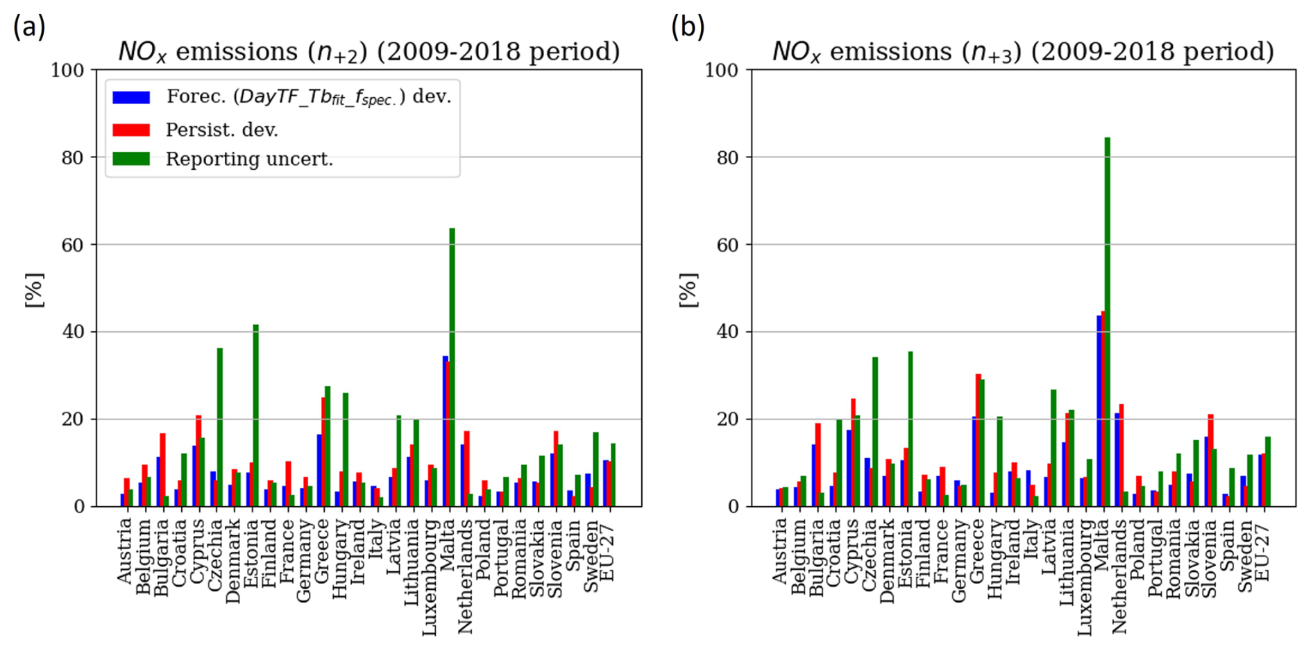
The average reporting uncertainty for NO_x emissions is 14.1 % up to 2 years (U₊₂) and 15.7 % up to 3 years (U₊₃) for the EU 27 average, being lower than for PM_2.5. However, it remains higher than the average difference induced by the HDD-based projections: 10.4 % for n₊₂ and 11.6 % for n₊₃ for the EU 27 average. At national level, the relative difference induced by DayTF_Tb_fit_f_spec. is lower than the respective uncertainty for 22 (20) countries in n₊₂ (n₊₃).

Figure 11 Average relative difference between reported emissions of PM_2.5 (CAMS-REG-AP-v5.1, GNFR_C) and projected emissions using the DayTF_Tb_fit_f_spec. method (blue bars), and projected emissions by persistence (red bars) for n₊₂ (a) and n₊₃ (b) by country over the 2009–2018 period. HDD-based projections are also compared to the estimated reporting uncertainty (green bars) between 2009 and 2018 for emission recalculations up to 2 years (U₊₂) and 3 years (U₊₃) (from CEIP, 2023).

Figure 12 Same as Fig. 11 for the NO_x emissions from GNFR_C.

5 Discussion and conclusions

Based on statistical information on household energy consumption, this paper provides country- and species-dependent parameters (Tb_fit(c) and f_spec.(c)) to derive HDD-based daily temporal factors to distribute PM and NO_x emissions from residential and commercial heating for EU 27 countries. Tb_fit(c), the threshold of ambient temperature at which building heating is activated and HDDs accumulated, is fitted with daily national domestic gas consumption data available over the period 2016–2021 for eight countries (ENTSOG, 2023) and interpolated to the other EU countries using the IDW approach. f_spec.(c), the non-temperature-dependent fraction of residential emissions, is calculated for each EU 27 country based on the fraction of energy consumed by households for space heating (Eurostat, 2023); with the natural gas energy type for $f_{{\mathrm{NO}}_x}\left(c\right)$ and the solid fuels for f_PM(c). It allows us to capture the specific behavioural characteristics of these countries well (residential heating being used at different ambient temperature comfort values and with different energy mixes, and for different home insulation standards).

Several experiments were designed: the first with a monthly temporal factor (MonthTF), the second based on daily variations using HDDs with parameters from the literature (DayTF_ref.), the third using HDDs with Tb_fit(c) (DayTF_Tb_fit), and the last using HDDs with Tb_fit(c) and f_spec.(c) (DayTF_Tb_fit_f_spec.). This work was designed to meet two objectives. We first aimed to assess the sensitivity of simulated PM_2.5, PM₁₀ and NO₂ surface concentration to the different experiments (as described above) and to identify the best parameterization compared to in situ observations. Simulations carried out with the CHIMERE model for 2018 have shown that the implementation of HDDs in the calculation of anthropogenic emissions from residential and commercial heating has an effect on PM_2.5, PM₁₀ and NO₂ surface concentrations mainly from March to October. The performance scores were calculated at observation stations from the AQ e-Reporting database for the different experiments. DayTF_Tb_fit_f_spec. significantly improves the temporal correlation of the daily average concentration of PM_2.5 and PM₁₀ during the winter season (JFM), with an average increase in the R coefficient of +0.11 compared to the simulation without HDDs (MonthTF) and by +0.05 compared to the simulation with HDDs using parameters from the literature (DayTF_ref.).

HDDs appear to have a fairly neutral effect on daily average concentration scores for the autumn season (OND). It should be noted that autumn 2018 was relatively warmer than normal across Europe, with no significant cold spells. The scores obtained over this period do not allow us to highlight the benefits of HDDs. Furthermore, autumn, and especially its first few months, is a period of transition between the non-heating and heating seasons, which can vary considerably from one European country to another. Several studies have highlighted the difficulty of reproducing the beginning of the heating period (and its end in early spring), and this also applies to the HDD method (e.g. Grythe et al., 2019; Ciais et al., 2022).

Analyses carried out on the February and March 2018 pollution episodes related to cold spells showed that HDDs were necessary for a more correct simulation of PM_2.5 and PM₁₀ concentration peaks. The DayTF_Tb_fit_f_spec. experiment increases the number of good detection of threshold exceedance by +11 % and +57 % for PM_2.5 and PM₁₀ respectively compared to MonthTF on European stations, while it decreases the number of missed alarms (−7 % and −9 %). The increase in number of false alarms remains limited (+3 % and +1 %). This shows that DayTF_Tb_fit_f_spec. induces a better temporal distribution of concentration levels both below and above the exceedance thresholds, with the best probability of detection among the other parameterizations tested.

Concerning NO₂ species, the effect of HDDs on the simulated concentrations is low. As the contribution of GNFR_C emissions to total anthropogenic emissions remains limited (9.1 % over the EU 27 CEIP, 2023), residential heating does not appear to be the main driver of NO₂ background concentrations, even during cold periods. Nevertheless, a significant decrease in the RMSE for the simulated concentrations in Italy, France, Hungary, Romania, Estonia and Latvia in winter was found, as well as a clear increase in good detection of threshold exceedance at the European level (+12 % with DayTF_Tb_fit_f_spec.).

Finally, it should be stressed that the country- and species-specific parameters proposed in this work for the HDD method are based on national statistics which may be characterized by a degree of uncertainty. For instance, Eurostat data may underestimate wood consumption during summer recreational activities (e.g. barbecues). Compiling data on wood consumption can be challenging, as it cannot be monitored in the same way as natural gas. Furthermore, not everyone within a country lives in equally well insulated houses or has the same socio-economic level that allows them to turn on the heating appliances when they want to.

The second aim of this article was to use HDDs as a method to model national emission totals from GNFR_C and compare them with persistence and uncertainty (estimated from the magnitude of emission recalculations in subsequent years). The DayTF_Tb_fit_f_spec. parameterization was chosen. The analyses presented in this document have shown that this method performs better in regards to emission uncertainties and therefore can be used to estimate the effect of multi-year variability in weather conditions to be taken into account, for both NO_x and PM emissions. The deviation obtained by the HDD projections is lower than the respective reporting uncertainty at the European level for both n₊₂ and n₊₃. The difference induced by HDD projections (compared with reported emissions) is even lower than with the persistence method (for more than half of the EU 27 countries).

The uncertainty estimated here is linked to changes in officially reported data at different years. The quality and accuracy of reported emissions data vary considerably from one country to another (EMEP, 2022). There are other ways of quantifying uncertainty in emissions inventories, for instance by including additional factors linked to the calculated emission factors or activity indicators. Kuenen et al. (2022) estimated that the uncertainty of GNFR_C in Europe is within the range 50 %–200 % for NO_x and 100 %–300 % for PM. The spatialization of emissions can also be associated with considerable uncertainties. As investigated in López-Aparicio et al. (2017) and Navarro-Barboza et al. (2024), wood combustion emissions may be over-allocated in urban areas compared to local inventories.

In conclusion, the HDD method shows positive results for the seasonal distribution and multi-year projection of emissions from commercial and residential heating. Based on the results of this paper, the use of HDDs and the spatialization of the parameters following the DayTF_Tb_fit_f_spec. experiment are recommended for the calculations of the emissions used as inputs in CTMs to improve the simulation of winter pollution episodes, including concentration peaks, but also for emission projections up to n₊₃. In addition, different emission scenarios can be designed based on the use of HDDs. The HDD approach could be used to assess and isolate the meteorological effects of other major societal events that may have an impact on air quality, such as an energy crisis or a lockdown due to a pandemic situation (e.g. Guevara et al., 2021a). Finally, future work could focus on the dynamical modelling of emissions from other sectors that also appear to incorporate a weather-dependent component in order to improve the modelling of pollutant concentrations, such as for the combustion of diesel engine or the spreading of salt/sand on roads.