Assessment of the 11-year solar cycle signals in the middle atmosphere during boreal winter with multiple-model ensemble simulations

To better understand possible reasons for the diverse modeling results and large discrepancies of the detected solar fingerprints, we took one step back and assessed the “initial” solar signals in the middle atmosphere based on a set of ensemble historical simulations with multiple climate models – the Flexible Ocean Climate Infrastructure (FOCI), the ECHAM/MESSy Atmospheric Chemistry (EMAC), and the Max Planck Institute for Meteorology Earth System Model in high-resolution configuration (MPI-ESM-HR). Consistent with previous work, we find that the 11-year solar cycle signals in the shortwave heating rate (SWHR) and ozone anomalies are robust and statistically significant in all three models. These initial solar cycle signals in the SWHR, ozone, and temperature anomalies are sensitive to the strength of the solar forcing. Correlation coefficients of the solar cycle with the SWHR, ozone, and temperature anomalies linearly increase along with the enhancement of the solar cycle amplitude. This reliance becomes more complex when the solar cycle amplitude – indicated by the standard deviation of the December–January–February mean F_10.7 – is larger than 40. In addition, the cold bias in the tropical stratopause of EMAC dampens the subsequent results of the initial solar signal. The warm pole bias in MPI-ESM-HR leads to a weak polar night jet (PNJ), which may limit the top-down propagation of the initial solar signal. Although FOCI simulated a so-called top-down response as revealed in previous studies in a period with large solar cycle amplitudes, its warm bias in the tropical upper stratosphere results in a positive bias in PNJ and can lead to a “reversed” response in some extreme cases. We suggest a careful interpretation of the single model result and further re-examination of the solar signal based on more climate models.

1 Introduction

Significant effects of the 11-year solar cycle on the middle-atmospheric temperature and constituents have been found in many observational and model studies in recent decades (e.g., see either Gray et al., 2010, or Ward et al., 2021 for a review). However, the modeled responses of the nitrogen dioxide (Hood and Soukharev, 2006; Wang et al., 2020), ozone (Soukharev and Hood, 2006; Swartz et al., 2012; Hood et al., 2015; Maycock et al., 2018), and stratospheric temperature (Mitchell et al., 2015; Matthes et al., 2017) in the middle atmosphere still show discrepancies among various models and observations. Enhanced absorption of solar UV radiation by ozone and oxygen in the middle atmosphere, with direct solar heating effect during the solar maximum years, can increase the tropical stratopause temperature. Kodera and Kuroda (2002) first proposed that the increase in the tropical stratopause temperature can strengthen the meridional temperature gradient and lead to an intensified polar night jet (PNJ) during wintertime. Anomalous westerly winds associated with the strengthened PNJ can propagate downward via interactions with the upward-propagating planetary waves. This proposed “top-down” mechanism was confirmed in subsequent studies with additional observational/reanalysis data (Kuroda et al., 2022) or with the aid of idealized simulations based on climate models (Matthes et al., 2006; Thiéblemont et al., 2015; Mitchell et al., 2015; Drews et al., 2022) but with various timing (Kodera and Kuroda, 2002; Drews et al., 2022; Kuroda et al., 2022). The solar signal may not be stationary (Thejll et al., 2003) and is modulated by internal climate variability, such as enhanced ozone and warming responses in the tropical lower stratosphere under the solar maximum, only found in the Quasi-Biennial Oscillation (QBO) east phase (Labitzke, 2005; Matthes and Walters, 2010), while the top-down propagation of the solar signal, and hence an intensified polar vortex at the surface, is much stronger in the negative phase of the Pacific Decadal Oscillation (Guttu et al., 2021).

Large discrepancies between the observed solar imprints and the modeling results (Li et al., 2016; Wang et al., 2020; Scaife et al., 2013; Andrews et al., 2015), as well as the inconsistent responses in climate models (Drews et al., 2022; Chiodo et al., 2019; Spiegl et al., 2023), diminish the robustness of the detected “solar signal” and call into question the proposed top-down mechanism and its surface response. The top-down mechanism, whereby the solar responses in the middle atmosphere trigger the downward coupling processes, was widely used to explain the solar influences on the Northern Hemisphere (NH) winter climate, especially the modulation on the North Atlantic Oscillation (NAO) (Kodera and Kuroda, 2005; Scaife et al., 2013; Andrews et al., 2015; Gray et al., 2016; Thiéblemont et al., 2015; Drews et al., 2022; Kuroda et al., 2022). However, the diverse modeling results, shown in the publications of Drews et al. (2022), Chiodo et al. (2019) and Spiegl et al. (2023), reduce the confidence level of the solar–NAO connection and the underlying mechanism. The uncertainties of the simulated solar responses in the middle atmosphere may partly explain the discrepancy of the solar surface imprints. In this study, we will use multiple-model ensemble simulations to evaluate the “initial” solar signals in the middle atmosphere with a consideration of the model stratospheric biases.

Kunze et al. (2020) quantified uncertainties of the 11-year solar signals in the annual-mean shortwave heating rates (SWHRs), temperature, and ozone anomalies in the middle atmosphere based on two chemistry–climate models (CCMs) – ECHAM/MESSy Atmospheric Chemistry (EMAC) and Community Earth System Model and Whole Atmosphere Chemistry Climate Model (CESM-WACCM). They found that the uncertainties of the solar responses in the SWHR, temperature, and ozone anomalies in the upper stratosphere–lower mesosphere arise mainly from the used solar spectral irradiance (SSI) dataset, but solar responses in the lower stratosphere also depend on the CCM used. Recent studies demonstrated that uncertainties of the solar-related dynamical responses in the stratosphere and troposphere, as well as the surface responses, are much larger than those of the initial solar signals in the middle atmosphere (Drews et al., 2022; Spiegl et al., 2023). A large spread in the dynamical responses, even with an opposite sign, has been found among individual ensemble members based on the same model and with identical solar forcing data (Spiegl et al., 2023). In addition, the stratospheric dynamic variability during the respective winter seasons in both hemispheres can also strongly influence the solar response in total column ozone at high latitudes in the models (Kunze et al., 2020). An evaluation of the 11-year solar signal in multiple-model ensemble simulations will update the information on the robustness and significance of solar imprints in Earth's atmosphere and also be helpful for the development of CCMs.

Although many studies show the importance of the middle atmosphere for the troposphere and surface climate, model representations of all the chemical, physical, and dynamic processes in the middle atmosphere are still a very big challenge (Scaife et al., 2022; Lawrence et al., 2022). Recently, longer predictability timescales of the stratosphere as compared to the troposphere have been identified (Tripathi et al., 2015; Butler et al., 2019; Domeisen et al., 2020a). The stratosphere and its coupling with the troposphere could be a source for the predictability of wintertime surface weather on subseasonal-to-seasonal (S2S) timescales (Hardiman et al., 2011; Jia et al., 2017; Domeisen et al., 2020b; Scaife et al., 2022). During the solar maximum years, the strong solar radiative effects in the upper stratosphere–lower mesosphere (direct heating and absorption of solar UV radiation) could change its thermal and dynamical features and hence influence the planetary wave propagation and reflection conditions in the lower stratosphere (Kodera and Kuroda, 2002; Matthes et al., 2006; Drews et al., 2022; Kuroda et al., 2022). Therefore, the quasi-decadal solar forcing is recognized as a potential source for near-term climate prediction (Scaife et al., 2022; Kushnir et al., 2019). However, climate models and forecast systems often struggle to correctly represent all stratospheric variability and their downward coupling processes (Scaife et al., 2016; Lawrence et al., 2022). The inclusion of the solar response in the middle atmosphere in a forecast system not only would improve the prediction of stratospheric events but also may help improve surface prediction skills.

Herein, we first assess the initial solar signals in the middle atmosphere (Sect. 3.1) as well as the top-down mechanism in multiple-model ensemble simulations (Sect. 3.2). Furthermore, we investigate the uncertainties of the dynamical responses in climate models with a consideration of the model biases (Sect. 3.3). In Sect. 2 we describe all three models and the setup of the experiments used in this study. In Sect. 3 we show the results, and in Sect. 4 we provide the conclusions and discussions.

2 Data and methods

2.1 Climate models

Three climate models are used in this study to assess the 11-year solar cycle signals in the middle atmosphere. They are the Flexible Ocean Climate Infrastructure (hereafter FOCI; Matthes et al., 2020), the ECHAM/MESSy Atmospheric Chemistry (hereafter EMAC; Jöckel et al., 2016), and the Max Planck Institute for Meteorology Earth System Model in high-resolution configuration (hereafter MPI-ESM-HR; Müller et al., 2018). A brief introduction of the three models is given below.

FOCI is a fully coupled CCM that includes the European Centre Hamburg general circulation model, sixth generation (ECHAM6.3) (Stevens et al., 2013), describing tropospheric and middle-atmospheric processes, coupled to the Nucleus for European Modelling of the Ocean version 3.6 (NEMO3.6) model (Madec, 2016), the JSBACH (Reick et al., 2013) land module, and the Louvain-la-Neuve Sea Ice Model (LIM2) (Fichefet and Maqueda, 1997). In the vertical, ECHAM6 consists of 95 hybrid sigma-pressure levels up to the model top at 0.01 hPa, and the Model for Ozone and Related Chemical Tracers (MOZART3; Kinnison et al., 2007) is implemented in ECHAM6 (ECHAM6-HAMMOZ; Schultz et al., 2018) to simulate the chemical processes in the atmosphere. The horizontal resolution of the atmosphere is approximately 1.8° by 1.8°, and the QBO can be internally generated. More details of FOCI can be found in Matthes et al. (2020).

The EMAC (ECHAM5 Version 5.3.02, MESSy Version 2.52) CCM integrates modules for tropospheric and middle atmospheric processes, including interactions with the ocean, land surfaces, and anthropogenic factors (Jöckel et al., 2010). Built on the Modular Earth Submodel System (MESSy2), EMAC links software codes from various institutes, and its core atmospheric model is the ECHAM5 (Roeckner et al., 2006). For the SOLCHECK project (https://romic2.iap-kborn.de/projekte/solcheck.html, last access: 14 February 2025), EMAC was operated in T42L47MA – with a spherical truncation of T42 (corresponding to a quadratic Gaussian grid of approx. 2.8° by 2.8° and a vertical resolution of 47 layers – with the model top at 0.01 hPa). Key submodels for SOLCHECK include MECCA (Sander et al., 2011) for atmospheric chemistry; J values for photolysis rates (Sander et al., 2014); Freie Universität Berlin Radiation (FUBRAD) for radiation transfer (Dietmüller et al., 2016); QBO (Giorgetta and Bengtsson, 1999); Upper Boundary Condition NOx (UBCNOx) for auroral influence (Funke et al., 2016); and MPIOM (Jungclaus et al., 2006) as an ocean component, operating at GR15L40 (Grid 1.5° and 40 Levels) resolution. To enhance spectral resolution in the UV–VIS range, the sub-submodel FUBRAD (Kunze et al., 2014) is utilized. This model is applied in the stratosphere and mesosphere at pressure levels below 70 hPa. Within this framework, FUBRAD uses a detailed subdivision of 81 spectral bands. These bands span the Lyman-α line (121.5 nm) and include key spectral features such as the Schumann–Runge bands and continuum (125.5–205 nm), the Herzberg continuum (206.2–243.9 nm), the Hartley bands (243.9–277.8 nm), the Huggins bands (277.8–362.5 nm), and the Chappuis bands (407.5–690 nm).

The MPI-ESM-HR (Müller et al., 2018) consists of the atmosphere model European Centre Hamburg Model of version 6.3 (ECHAM6.3; Stevens et al., 2013) at approximately 100 km horizontal resolution and with 95 levels in the vertical up to the top at 0.01 hPa (T128L95). It is coupled to the Max Planck Institute Ocean Model of version 1.6.3 (MPIOM; Jungclaus et al., 2013) with a tripolar grid of about 0.4° and 40 vertical levels. Additional components of MPI-ESM-HR are the ocean biogeochemical model Hamburg Model of the Ocean Carbon Cycle (HAMOCC; Ilyina et al., 2013) and the land surface model Jena Scheme for Biosphere Atmosphere Coupling in Hamburg (JSBACH; Reick et al., 2013). It is worth noticing that the MPI-ESM-HR is not a CCM. Ozone concentrations from the CMIP6 are used in this model, and the ozone is treated inactively.

2.2 Experimental design

Two sets of CMIP6 historical-like ensemble simulations are performed with the three climate models (i.e., FOCI, EMAC, and MPI-ESM-HR) driven by identical external forcing as recommended for CMIP6 (Eyring et al., 2016), except for the solar forcing. The first ensemble, named FULL in this study, includes full solar variability using the CMIP6 solar forcing dataset (Matthes et al., 2017). The second ensemble called FIX serves as a reference experiment, in which the solar forcing is fixed to 1850 preindustrial conditions. All ensemble simulations based on the three models have been integrated over the historical period 1850–2014, and the individual ensemble members have been initialized from different model years of a multi-centennial pre-industrial control simulation. A total of 9 members of the FULL ensemble are performed with FOCI, 6 members with EMAC, and 10 members with MPI-ESM-HR. Thus, a total of 25 members and 4125 model years of the FULL ensemble have been analyzed in this study. The number of ensemble members of FIX is identical to the FULL ensemble, except for 8 members with MPI-ESM-HR. In this study, we mainly focus on assessing the 11-year solar signal in the middle atmosphere using the FULL ensemble and comparing it to the FIX ensemble at some points.

To validate our model results, 3D temperature and zonal wind from the ECMWF Reanalysis v5 (ERA5; Hersbach et al., 2020) covering 1950 to the present are used. The annual-mean and December–January–February mean (DJF-mean) F_10.7 radio flux in the solar flux units (1 sfu = 10⁻²² W m⁻² Hz⁻¹) from the CMIP6 soar forcing dataset (Matthes et al., 2017) is used as an index for solar variability.

2.3 Analysis methods

To investigate the persistence of the solar imprints, we calculate correlation coefficients (CCRs) within a 45-year running window between the solar index F_10.7 and several meteorological variables (e.g., SWHR, temperature, ozone volume mixing ratio, and zonal wind). We note that this method will reduce the overall signal-to-noise ratio compared to the response derived from the full period as only four adjacent solar cycles are involved in each window. A standard deviation of the annual-mean and DJF-mean F_10.7 index in the 45-year running window are used to indicate the mean strength of solar variability in that “time” window (called solar cycle amplitude hereafter). A scatter diagram of the correlation coefficients and the solar cycle amplitudes in all 121 windows is used to demonstrate the possible reliance of the solar imprint on the strength of solar variability. Similarly, the models' biases of wind speed and temperature in the 45-year running windows are scattered together with the correlation coefficients to show the possible dependence of the solar imprint on the model bias in the middle atmosphere. The models' biases are defined by the differences between the model climatology averaged in the 45-year running window and the ERA5 climatology – an average of 1950–2014. Here, we note that the climate states in the 45-year windows could shift among the different historical periods and, thereby, a large uncertainty in the model biases for the earlier period by being compared to the ERA5 climatology of 1950–2014; more discussion can be found in Sect. 3.3. The 95 % significance level for the correlation coefficient was calculated based on a two-tailed Student's t test, and the effective degrees of freedom in a 45-year window are calculated following the method used in the work of Pyper and Peterman (1998) and simplified as only the autocorrelation coefficients at lag 1 are considered. More details of this method are also described in the work of Huo et al. (2023). In addition, when 80 % of ensemble members agreed on the sign of the correlation coefficient, we interpreted it as a robust response.

Composites of the meteorological variables based on the 11-year solar cycle are generated by calculating differences between the average values in all solar maximum years and minimum years. Here the solar maximum (minimum) years are defined following the method used in the work of Drews et al. (2022); i.e., the solar maximum (minimum) for each solar cycle includes 3 years – the year of the peak (valley) and 2 years around it. A 1000-fold bootstrapping test with replacement (Diaconis and Efron, 1983) is used to estimate the 90 % statistical significance of the ensemble mean composites. The meridional temperature gradient is calculated by performing a centered finite difference operation on the latitude dimension. Here we use annual-mean data to examine the direct solar signal in the SWHR, temperature, and ozone volume mixing ratio anomalies. Then, we focus on the NH extended winter season (from November to March) to investigate the possible resulting dynamic responses. For each meteorological variable from individual ensemble members and the observation, its least-squares quadratic trend and the mean value of the whole data period are removed to get its detrended anomaly.

3 Results

3.1 Initial 11-year solar signals in the middle atmosphere

The incoming solar radiation absorbed by the Earth's middle and upper atmosphere directly influences the SWHR, temperature, and ozone production in the sunlit region with the strongest effects in the tropics. Although solar UV radiation accounts for only a small part of the solar spectrum at the top of the atmosphere (approximately 8.73 %) (Gueymard, 2004), it has a larger variation (of up to 6 %) between the solar maximum and minimum of the 11-year solar cycle than the total solar irradiance (be about 0.07 %) (Gray et al., 2010). Figure 1 shows the composite difference between the solar maximum and minimum of the annual-mean SWHR, temperature, and ozone anomalies. All three models used in this study can simulate significant responses of the SWHR, temperature, and ozone in the tropical upper stratosphere to the 11-year solar cycle. However, maximum responses of the ensemble mean SWHR, temperature, and ozone anomalies in this study (solid lines in Fig. 1) are a quarter smaller than the previous found in Matthes et al. (2017). Different chemistry schemes (as described in Sect. 2.1) and shortwave radiation codes implemented in FOCI and EMAC could be one of the potential reasons for the various SWHR and temperature responses in the two CCMs. Although the parameterization of radiative transfer in the mesosphere (layers at pressures lower than 70 hPa) could be improved by increasing the spectral resolution of Lyman-α from 1 band to 81 bands in the RAD-FUBRAD submodule of EMAC (Nissen et al., 2007), the maximum response of SWHR at the tropical stratopause (Fig. 1a) is dominated by the Hartley bands and Huggins bands (Sukhodolov et al., 2014). Differences in the radiation codes of ECHAM5 (Version 5.3.02, used in EMAC) and ECHAM6 (Version 6.3, used in FOCI) could be one of the reasons for the different responses in these two CCMs (Sukhodolov et al., 2014). In addition, the composite method used in our study (as described in Sect. 2.3) and the ensemble mean of multiple transient simulations reduce part of the aliasing of solar signal with the high-frequency inter-annual variability and internal variability, leading to an “underestimated” solar signal in this study compared with previous works with idealized sensitivity simulations (e.g., Matthes et al., 2017; Kunze et al., 2020) or a multiple linear regression method (e.g., Spiegl et al., 2023; Mitchell et al., 2015). The large spread of the response over the period (shadow regions), i.e., various responses among different solar cycles, suggests the detected solar signal could be very different when focusing on different solar cycles.

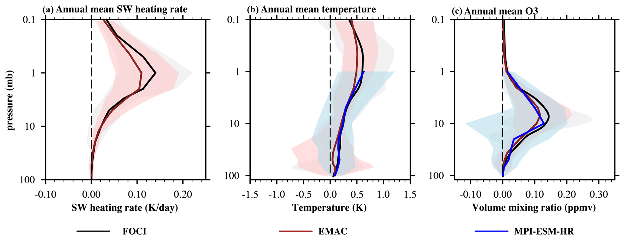
Figure 1 Composite differences between solar maxima and minima of the tropical (averaged over 25° S–25° N) annual (a) shortwave heating rate anomalies, (b) temperature anomalies, and (c) O₃ volume mixing ratio anomalies in the FULL ensemble mean with respect to the FIX ensemble mean. Here black lines indicate the ensemble mean temperature anomalies of FOCI, brown lines are EMAC, and blue lines are MPI-ESM-HR. The light-gray shadow regions indicate the response spread over the period for FOCI. Light-pink and light-blue shadow regions are for EMAC and MPI-ESM-HR, respectively.

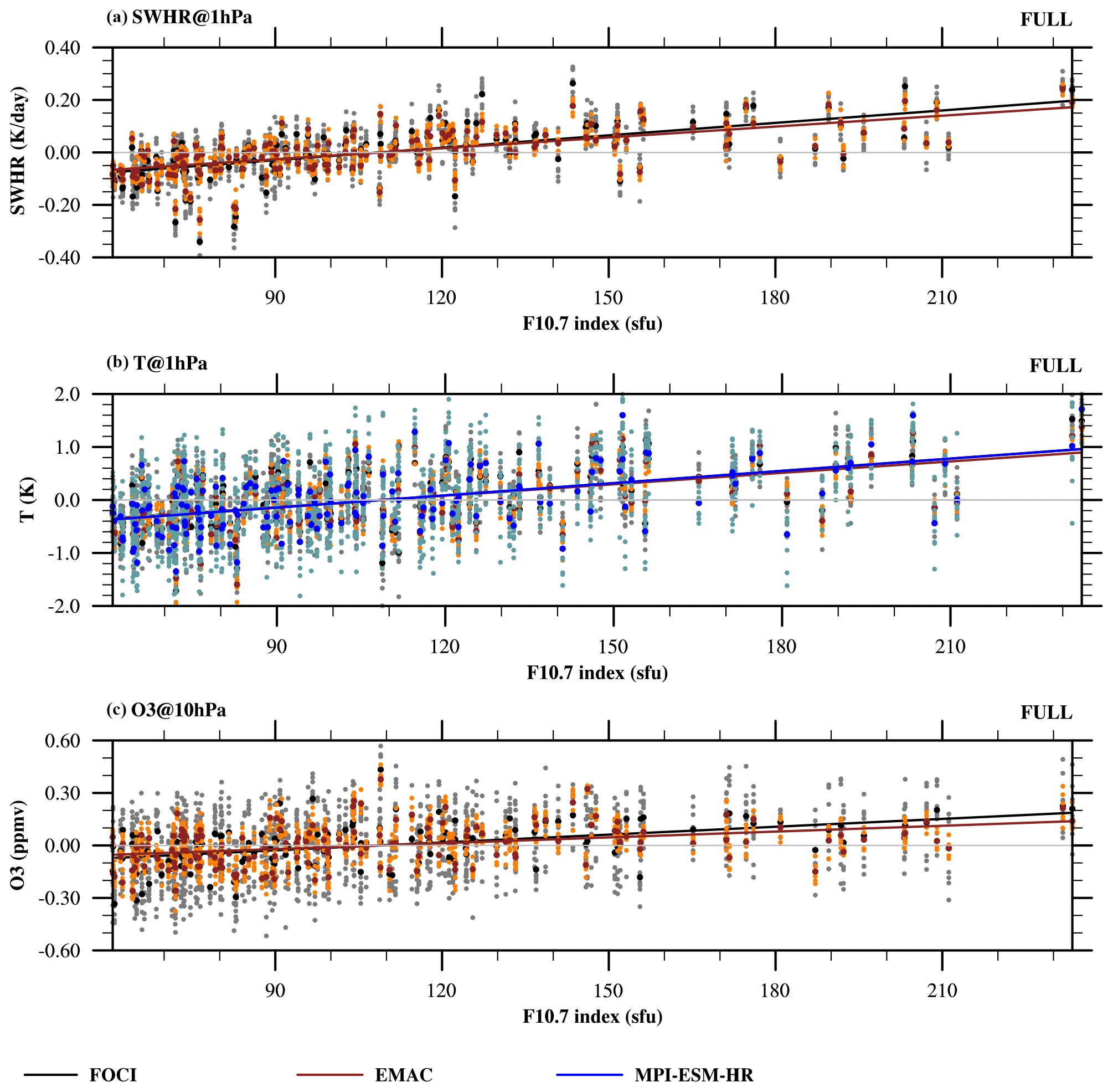
Figure 2 Direct solar signatures in the upper stratosphere. (a) Scatter diagram of the annual-mean shortwave heating rate (SWHR) anomalies (units: K d⁻¹) at the tropical stratopause (averaged over 25° S–25° N at 1 hPa) vs. the annual F_10.7 index from the FULL experiment with FOCI (black: ensemble mean; light gray: individual members) and EMAC (brown: ensemble mean; light brown: individual members). (b) As (a) but for the annual temperature at 1 hPa (K) from FOCI, EMAC, and MPI-ESM-HR (blue: ensemble mean; light blue: individual members). (c) As (a) but for the annual ozone volume mixing ratio (ppmv) at 10 hPa from FOCI and EMAC.

Figure 2 shows a scatter diagram of the annual-mean SWHR (Fig. 2a) and temperature (Fig. 2b) anomalies at the tropical stratopause (around 1 hPa) in the FULL experiment vs. annual-mean F_10.7. Here, we should note that the direct solar signal in the SWHR and ozone anomalies in MPI-ESM-HR are not shown here because the ozone response is prescribed and the SWHR output is not available. As expected, the SWHR, temperature, and O₃ increase along with the enhancement of solar radiation in all models and most ensemble members, indicated by linear trend lines in Fig. 2. Please note that the anomaly of the meteorological variable (i.e., SWHR and temperature here) is defined as its deviation from the detrended mean value of the whole period, so the 0 value of the y axis of Fig. 2 indicates that the value of that data point has no deviation from the mean value. More positive anomalies of the SWHR and temperature at approximate F_10.7 ≥ 140 sfu suggest a possible solar impact when solar radiation is large. Most members from FOCI and EMAC show positive SWHR and temperature anomalies with fluctuating deviations at F_10.7 ≥ 180 sfu. A very similar characteristic is also found in the ozone response at 10 hPa (as shown in Fig. 2c). The above responses of the SWHR, temperature, and ozone anomalies to the solar radiative forcing are absent in the FIX experiment (as shown in Fig. A1). The waved positive responses in the tropical stratopause (SWHR and temperature) at F_10.7 ≥ 180 sfu may imply a nonlinear response when the solar forcing is strong enough. However, compared with the FIX experiments, the analogous fluctuation in the SWHR and temperature responses at the F_10.7 ≥ 180 sfu also implies a robust fingerprint of other external forcings in the tropical stratopause, in addition to the solar forcing. The large spread and fewer samples of the strong solar cycles should be noted (e.g., indicated by F_10.7 ≥ 180 sfu in Fig. 2).

The different behavior of the SWHR, temperature, and ozone anomalies in the FULL and FIX experiments (Figs. 2 and A1) indicates significant solar fingerprints in the tropical upper stratosphere. To examine the solar influence in the middle atmosphere at the decadal timescale (i.e., the signal of the 11-year solar cycle) as well as its stability, we calculate the correlation coefficients of the F_10.7 index with SWHR, temperature, and ozone anomalies in a 45-year running window from 1850 to 2014. As shown in Fig. A2a, a significant and robust 11-year solar signal exists in the SWHR anomalies averaged over the tropical stratopause with a very small ensemble spread for all models. However, the resulting temperature anomalies in the tropical stratopause for all models have a weaker positive correlation with the F_10.7 in the 45-year windows than the SWHR anomalies, which is significant in the later period after 1920 (Fig. A2b). The larger ensemble spread in the earlier period (before 1920) indicates a strong disturbance of the internal variability on solar imprints in the tropical stratopause temperature. The 11-year solar signal in the tropical ozone anomalies at 10 hPa is significant and robust in all the 45-year running windows for both FOCI and EMAC (Fig. A2c).

Figure 3 Initial 11-year solar cycle signals in the upper and middle stratosphere vs. the solar cycle amplitude. (a) Scatter plot of correlation coefficients between the annual shortwave heating rate anomalies in the tropical stratopause (averaged over 25° S–25° N at 1 hPa) and the annual F_10.7 index in all 45-year running windows vs. the solar cycle amplitude (standard deviations of the annual F_10.7 index in all 45-year windows) for FOCI (ensemble mean: black; light gray: individual members) and EMAC (brown: ensemble mean; light brown: individual members) in the FULL experiment. The dashed black line indicates the 95 % significance level. Panel (b) is the same as (a) but for the temperature anomalies at 1 hPa from FOCI, EMAC, and MPI-ESM-HR (blue: ensemble mean; light blue: individual members). Panel (c) is the same as (a) but for the O₃ volume mixing ratio anomalies at 10 hPa from FOCI and EMAC.

Figure 3a shows some reliance of the detected solar signal on the solar cycle amplitude by a scatter distribution of the correlation coefficients of the F_10.7 index and the SWHR anomalies vs. the standard deviation (SD) of the F_10.7 index in all 45-year windows. A significant and robust 11-year solar signal in the SWHR anomalies (i.e., positive correlation coefficients) can be achieved in all members and all models in all 45-year windows (Fig. 3a). However, the positive responses in the temperature anomalies at 1 hPa (Fig. 3b) and ozone anomalies at 10 hPa (Fig. 3c), indicated by the positive correlation coefficients, are only significant and robust when the SD of F_10.7 index is larger than 28. These positive responses in SWHR, temperature, and ozone anomalies linearly increase along with the enhancement of the solar cycle amplitude when the solar cycle amplitude is smaller than 40. This linear reliance of the detected solar signal on the solar cycle amplitude turns into nonlinear features for all the models when the solar cycle amplitude is larger than 40; i.e., although the solar cycle amplitudes are identical in some 45-year windows, different correlation coefficients between the F_10.7 index and the SWHR, temperature, and ozone anomalies in these windows could be achieved. All the correlation coefficients are above the 95 % significance level at SD ≥ 40, and the solar signal is more prominent in the ensemble mean. Please note that the ensemble mean in this study (e.g., large dots in Fig. 3) is the correlation of the ensemble mean temperature (also SWHR and ozone) anomalies with the F_10.7 index, not the ensemble mean of correlations of single ensemble members with the solar index.

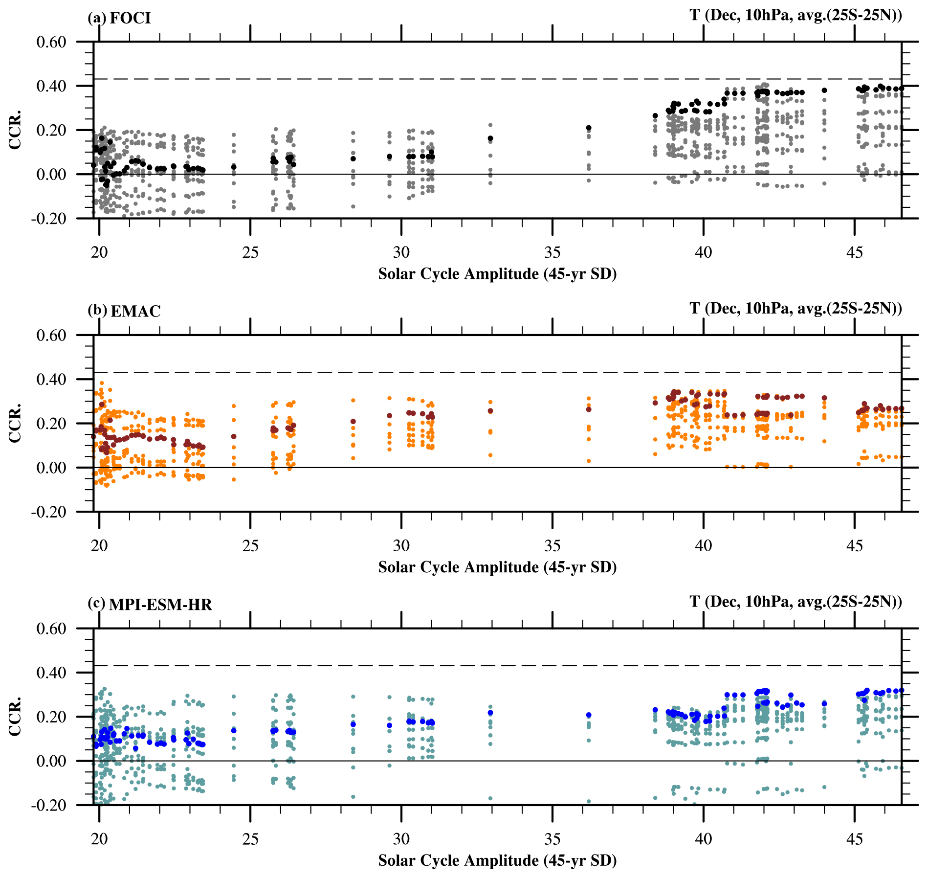
Figure 4 The 11-year solar cycle signals in the middle-stratospheric temperature anomalies vs. the solar cycle amplitude. Scatter plots of correlation coefficients between the temperature anomalies in December averaged over 25° S–25° N at 10 hPa and the DJF-mean F_10.7 index in all 45-year running windows vs. the solar cycle amplitude for (a) FOCI (black: ensemble mean; light gray: individual members), (b) EMAC (brown: ensemble mean; light brown: individual members), and (c) MPI-ESM-HR (blue: ensemble mean; light blue: individual members) in the FULL experiment. The dashed black line indicates the 95 % significance level.

We performed a similar analysis for the December temperature anomalies in the middle stratosphere (i.e., temperature anomaly at 10 hPa), which is partly related to solar-induced ozone anomalies. Although all three models simulated a positive temperature response in the ensemble mean (large dots in Fig. 4, none of them passes the 95 % significance level in all the 45-year windows. The temperature anomalies at 10 hPa in FOCI and MPI-ESM-HR only have robust positive correlations (i.e., 80 % of the ensemble members show positive correlation coefficients) with the DJF-mean F_10.7 index when the solar cycle amplitude is larger than 30, while no apparent reliance exists in EMAC. Therefore, different from the direct solar signals in the tropical stratopause, the temperature response in the middle stratosphere (i.e., 10 hPa in this study) is much weaker. It seems model-dependent and could be influenced by strong internal variability, like QBO and the El Niño–Southern Oscillation.

3.2 The top-down mechanism in multiple-model ensemble simulations

According to previous work, the tropical upper-stratospheric warm response to the solar cycle is expected to lead to an increased meridional temperature gradient and hence a so-called top-down dynamical response during the NH winter season (Kodera and Kuroda, 2002; Matthes et al., 2006; Drews et al., 2022; Kuroda et al., 2022). However, inconsistent results of the solar UV-forcing have been demonstrated in previous single-model studies, including various timings in the middle atmospheric response and an unstable solar–NAO connection. In this subsection, we re-examine the top-down mechanism with our multiple-model ensemble simulations.

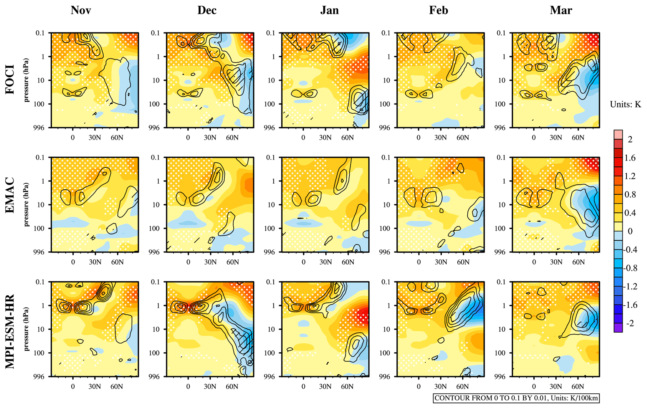
Figure 5 Zonal-mean temperature anomaly response to the 11-year solar cycle forcing during the extended winter season (from November to March). Composite differences between solar maximum and minimum of the ensemble mean zonal-mean temperature anomalies (units: K, color shading contours) and the poleward meridional temperature gradients (units: K (100 km)⁻¹, contours) from the FULL experiment with FOCI (top panels), EMAC (middle panels), and MPI-ESM-HR (bottom panels). Latitude–height cross sections are from 30° S to 90° N and 996 to 0.1 hPa. Only the positive meridional temperature gradient anomalies (poleward) are shown here. The 90 % significance level for the composite of temperature (meridional gradients) anomalies is indicated by white dots (black hatching) based on a 1000-fold bootstrapping test.

Figure 5 shows composite differences between the solar maximum and minimum of the ensemble mean zonal-mean temperature anomalies and the anomalous poleward temperature gradients in the FULL experiment. All three models used in this study capture the significant warm response in the tropical and subtropical lower mesosphere and upper stratosphere (color shading contours in Fig. 5) during the extended winter season (i.e., from November to March). The solar-induced tropical stratopause warming is stronger in FOCI (first row of Fig. 5) than in EMAC (second row of Fig. 5), which is highly related to the SWHR response in the atmosphere layers above approximately 4 hPa (as shown in Fig. A3). In addition, a non-significant lower-stratosphere warm response around 70 hPa is observed in FOCI (first row of Fig. 5) and MPI-ESM-HR (third row of Fig. 5), but it disappears in EMAC (second row of Fig. 5). Previous work suggested the lower-stratosphere warm response is an indirect effect of the maximum solar forcing, involving changes in the ozone chemistry and the Brewer–Dobson circulation (Kodera and Kuroda, 2002; Mitchell et al., 2015) and nonlinear interference with internal variability (e.g., the QBO). However, this secondary weak warming could also be an aliasing of a residual volcanic signal or some surface signals (Chiodo et al., 2014; Kuchar et al., 2017).

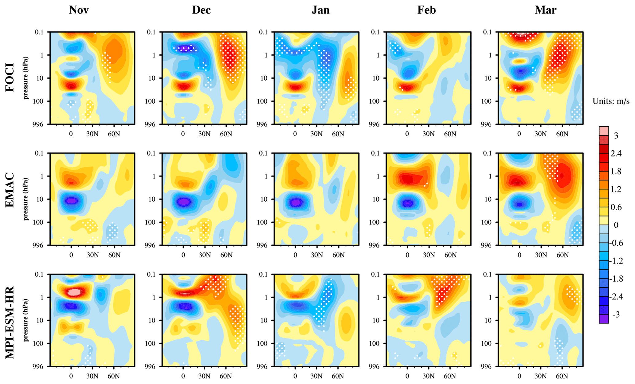
Figure 6 Zonal-mean zonal wind anomaly response to the 11-year solar cycle forcing during the extended winter season (from November to March). The same as Fig. 5 but for the ensemble mean zonal-mean zonal wind anomalies (units: m s⁻¹) in the FULL experiment for FOCI (top), EMAC (middle), and MPI-ESM-HR (bottom).

Although the upper-stratospheric warm response appears in the tropics and subtropics for all three models, the resulting changes in the meridional temperature gradient are quite different, as shown by the contours in Fig. 5. The anomalous poleward meridional temperature gradients increase in the lower mesosphere and upper stratosphere subtropics during all winter months in FOCI (first row of Fig. 5), which are weaker in EMAC (second row of Fig. 5) due to its weaker responses of the tropical stratospheric SWHR and temperature anomalies. The meridional temperature gradient anomalies in the NH high latitude and polar region increase in FOCI during the November–December–January with a poleward and downward movement. A similar and weaker response of the temperature gradient anomaly also shows up in the FULL experiment with MPI-ESM-HR (third row of Fig. 5) but not in EMAC (second row of Fig. 5). As a result of the enhancement of the poleward meridional temperature gradient, anomalous westerly winds in the NH high latitude and polar region can be found during November–December–January in both FOCI and MPI-ESM-HR (Fig. 6). It is worth noting that the enhanced meridional temperature gradient in the stratosphere in March (contours in the right column of Fig. 5) leads to a stronger stratospheric polar night jet for all three models (right column of Fig. 6). The conformity of the meridional temperature gradient anomalies and zonal-mean zonal wind anomalies suggests a dominant role of the thermal-wind relationship in the middle atmosphere. The downward movements of the zonal-mean meridional temperature gradient anomalies and the zonal-mean zonal wind anomalies in the polar vortex region from November to January could be a result of the interaction between the mean flow and upward planetary waves (Kodera and Kuroda, 2002; Matthes et al., 2006).

Drews et al. (2022) proposed that the statistically significant top-down propagation of the 11-year solar cycle signal and its surface imprints can only be detected in an epoch with strong solar cycle amplitude (1932–2014) based on the CESM-WACCM. However, this point could not be confirmed in the study of Spiegl et al. (2023), who analyzed a set of historical simulations with the MPI-ESM-HR contribution forced with CMIP5 data. As the solar signals in the FULL experiment with FOCI seem to be sensitive to the magnitude of solar cycle forcing (Figs. 3 and 4a), we repeated the above composite analysis for FOCI for the same weak and strong epochs as defined in the work of Drews et al. (2022). As shown in Figs. A4 and A5, both the zonal-mean ozone and temperature anomalies show a larger response in the strong epoch than in the weak epoch for the extended winter season. The significant enhancements of the meridional temperature gradient anomalies are confined in the middle atmosphere (above the tropopause), and no clear top-down migration of the signals is found in the weak epoch (contours in the first row of Fig. A5). The top-down mechanism is confirmed in the strong epoch such that both the positive meridional temperature gradient anomalies (contours in the second row of Fig. A5) and the resulting zonal-mean zonal wind anomalies (second row of Fig. A6) are transferred from the stratosphere to the surface during the extended winter season (November–February). The different responses in the weak and strong epochs with FOCI are in line with the work of Drews et al. (2022). However, this feature cannot be found in the FULL experiment with EMAC and MPI-ESM-HR, implying a model dependence of the simulated solar response. Previous studies show that it is necessary to group the data according to the QBO phases to find a clear 11-year solar signal in the middle to lower stratosphere (Labitzke and van Loon, 2000; Labitzke, 2005; Matthes and Walters, 2010). In this study, both FOCI and MPI-ESM-HR have an internally generated QBO; therefore the aliasing of QBO with the solar signal is expected to be largely reduced in the ensemble mean composite based on the solar cycle. However, the QBO-like signal still can be observed in FOCI (first row of Fig. 6) with the average of nine ensemble members, which is much weaker in MPI-ESM-HR (third row of Fig. 6). This residual QBO signal can influence the presentation and propagation of solar signals in the middle to lower stratosphere. An interesting feature is that the observed QBO west phase in the composite of zonal-mean zonal wind in FOCI (first row of Fig. 6) is more significant and pronounced during the weak epoch (first row of Fig. A6) and is less prevalent in the strong epoch (second row of Fig. A6). Except for the weaker solar forcing in the weak epoch than in the strong epoch, the QBO west “residual” signal in FOCI also results in fewer net ozone and temperature changes during the weak epoch.

3.3 Model-dependent dynamical responses to the 11-year solar cycle forcing

As demonstrated by Fig. 6, responses in the stratospheric zonal-mean zonal wind anomalies show a large diversity between multiple models. To further explore possible reasons for the simulated “inconsistent” dynamical responses in the middle atmosphere, here we use the zonal-mean zonal wind anomalies averaged over 60–65° N at 1 and 10 hPa to approximately indicate the PNJ anomalies in the upper and middle stratosphere. Figure 7 shows the scatter plots of correlation coefficients between December PNJ anomalies and the F_10.7 index vs. solar cycle amplitudes in all 45-year running windows. Although none of the correlation coefficients is above the 95 % significant level, most of the ensemble members as well as the ensemble mean show positive correlation coefficients of the PNJ anomalies with the F_10.7 index when the solar cycle amplitude is larger than 28. This result suggests the significant warming response in the tropical stratopause (Fig. 3b) could result in a strengthened PNJ, and the solar signal is much weaker compared to the internal variability. We should also note the manifestly negative correlation coefficients in FOCI and MPI-ESM-HR (Fig. 7a and c) but positive correlation in EMAC (Fig. 7b) when the solar cycle amplitude is very small (e.g., SD = 20). These opposing model results suggest that weak solar activity leading to a weak temperature response is no longer dominant in the correlation between the PNJ and the solar cycle, and the effects of other internal variability become visible, leading to a very large model spread. The positive correlation coefficients of the PNJ anomalies and the F_10.7 also show a nonlinear reliance on the solar cycle amplitude at SD ≥40 for all three models, which is consistent with the significant and multiplex positive temperature response at the SD ≥ 40 (Fig. 3b).

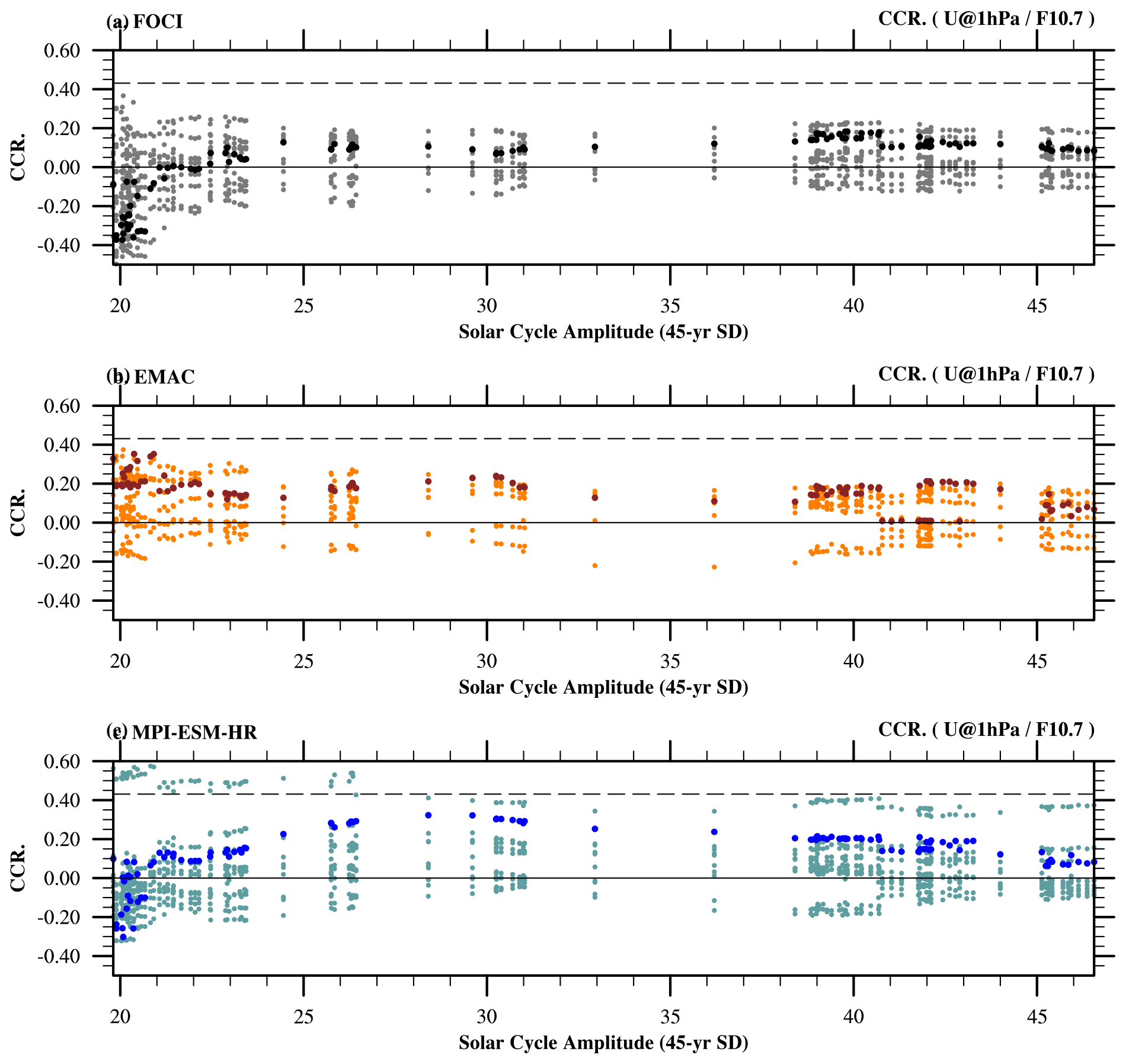
Figure 7 Upper-stratospheric polar night jet anomaly response to the solar forcing vs. the solar cycle amplitude. Scatter plots of correlation coefficients between the December zonal-mean zonal wind anomalies averaged over 60–65° N at 1 hPa and the DJF-mean F_10.7 index in all 45-year running windows vs. the solar cycle amplitude for (a) FOCI (black: ensemble mean; light gray: individual members), (b) EMAC (brown: ensemble mean; light brown: individual members), and (c) MPI-ESM-HR (blue: ensemble mean; light blue: individual members). The dashed black line indicates the 95 % significance level.

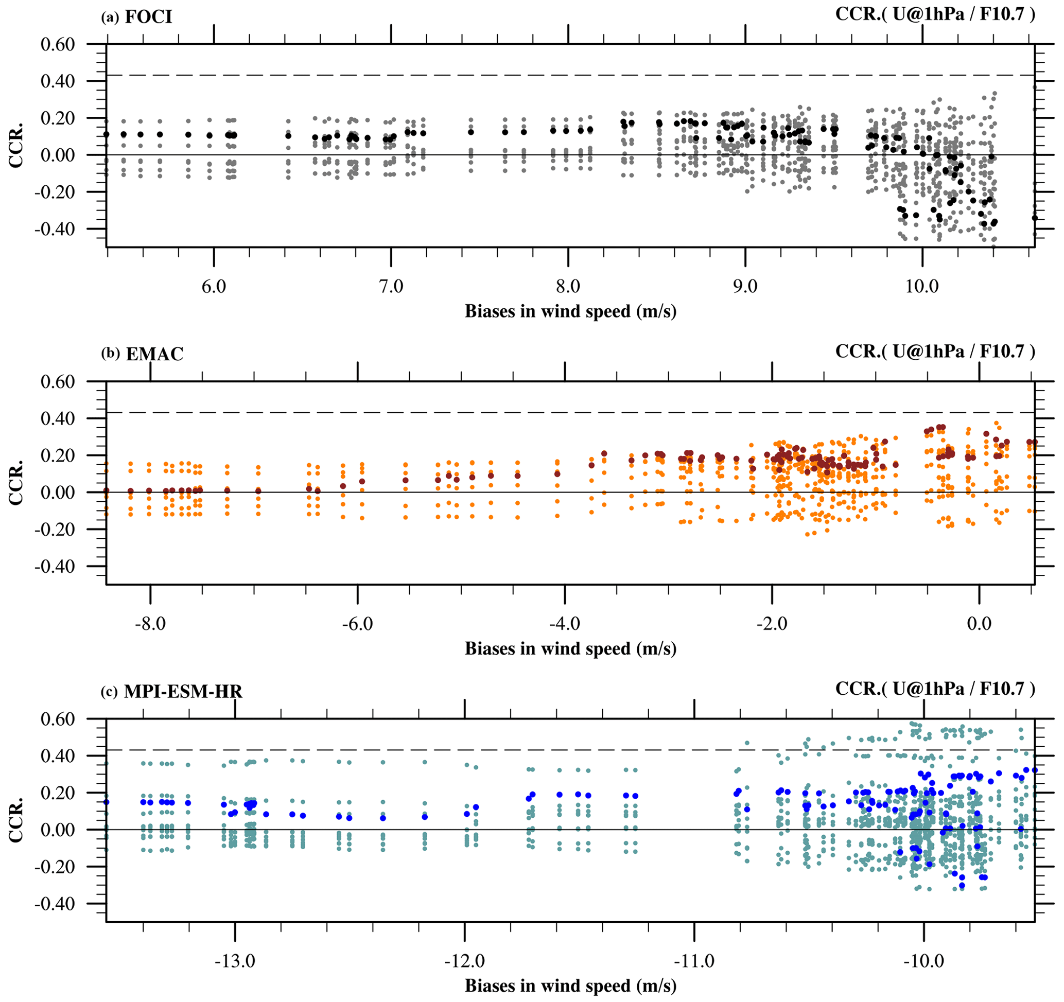
Figure 8 Upper-stratospheric polar night jet responses to the solar forcing vs. biases of the mean flow strength. Scatter plots of correlation coefficients between the December zonal-mean zonal wind anomalies averaged over 60–65° N at 1 hPa and the DJF-mean F_10.7 index vs. the biases of wind speed averaged over 60–65° N at 1 hPa in all 45-year windows for (a) FOCI (black: ensemble mean; light gray: individual members), (b) EMAC (brown: ensemble mean; light brown: individual members), and (c) MPI-ESM-HR (blue: ensemble mean; light blue: individual members). The dashed black line indicates the 95 % significance level.

As supposed in Spiegl et al. (2023), the background states of the middle atmosphere may play a role in the initial solar signal transfer. To explore this point, we plotted the correlation coefficients between the December PNJ anomalies and the F_10.7 index vs. the PNJ strengths, as shown in Fig. 8. Compared to the mean wind speed from the ERA5, both EMAC and MPI-ESM-HR have a weaker PNJ (the negative biases in the zonal wind speed in Fig. 8b and c), while it is stronger in FOCI (positive biases in the zonal wind speed in Fig. 8a). The positive and negative correlation coefficients from all ensemble members and all 45-year windows in FOCI and MPI-ESM-HR are distributed evenly regardless of the wind speed, showing very little sensitivity of the PNJ response to the PNJ strength in these two models. The negative correlation coefficients of ensemble mean zonal wind anomalies in FOCI (black dots) and MPI-ESM-HR (blue dots) indicate a weakened PNJ response, opposite to the proposed top-down mechanism. These “unexpected” dynamical responses under too strong (or too weak) a PNJ background condition with FOCI (MPI-ESM-HR) imply that the model bias may lead to a false representation of the solar signal. The model dependence of the PNJ response is also revealed in EMAC (Fig. 8b), where a robust and strengthened PNJ response appears when the simulated wind speed is close to the observed value (i.e., small model biases). Please note that the model biases in this study were estimated by comparing the model climatology of the 45-year running windows with the ERA5 climatology of 1950–2014. Therefore, when the 45-year window does not overlap with the ERA5 period, the model “bias” estimated in this 45-year window involves both a true model bias and a difference of climate states. Although the different climate states in the earlier periods from the ERA5 period can offset the estimation of model biases, the negative (positive) biases of the stratospheric zonal mean zonal wind in the polar vortex region for the common period of the ERA5 climatology (Fig. A7d–f) confirm the weaker (stronger) PNJ in EMAC and MPI-ESM-HR (FOCI) found in most 45-year windows (Fig. 8a–c).

Here we calculated the zonal mean meridional temperature gradient (ΔT) at 1 and 10 hPa using the mean value of the tropical box (25° S–25° N) minus the mean value of the polar box (65–90° N) for all three models (Table 1). The simulated meridional temperature gradients at 1 hPa in all three models (first row of Table 1) are weaker than the ERA5 (ΔT=19.1 K), especially for the MPI-ESM-HR model, where ΔT is just 7.8 K. The ΔT value at 10 hPa in FOCI and EMAC (second row of Table 1) is close to the value in ERA5 (ΔT=23.6 K), but it is still too weak in MPI-ESM-HR. The negative biases of the meridional temperature gradients in EMAC and MPI-ESM-HR could be a reason for the weak PNJs in these models.

Table 1 Meridional temperature gradients ΔT (units: K) in climate models and the ERA5 for a common period of 1950–2014.

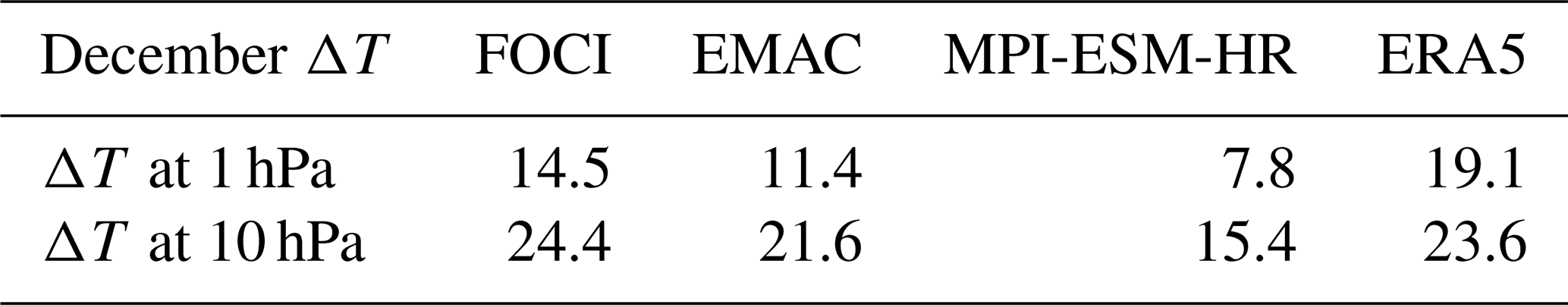
ΔT is calculated by the mean value of the zonal mean temperature in the tropics (25° S–25° N) minus the mean value in the pole zone (65–90° N).

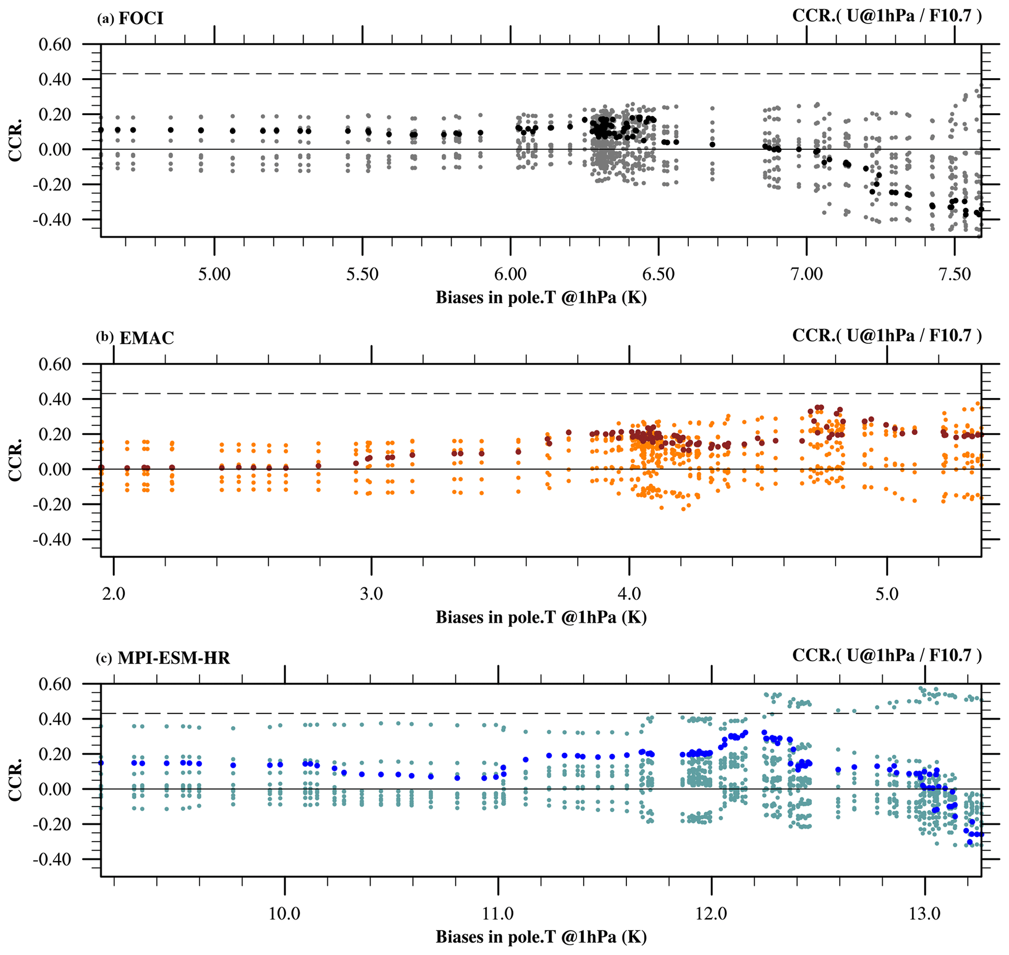
Figure 9 Upper-stratospheric polar night jet responses to solar forcing vs. biases of the polar stratopause temperature. Scatter plots of correlation coefficients between the December zonal-mean zonal wind anomalies averaged over 60–65° N at 1 hPa and the F_10.7 index vs. biases of the temperature averaged over 65–90° N at 1 hPa in all the 45-year windows for (a) FOCI (black: ensemble mean; light gray: individual members), (b) EMAC (brown: ensemble mean; light brown: individual members), and (c) MPI-ESM-HR (blue: ensemble mean; light blue: individual members).

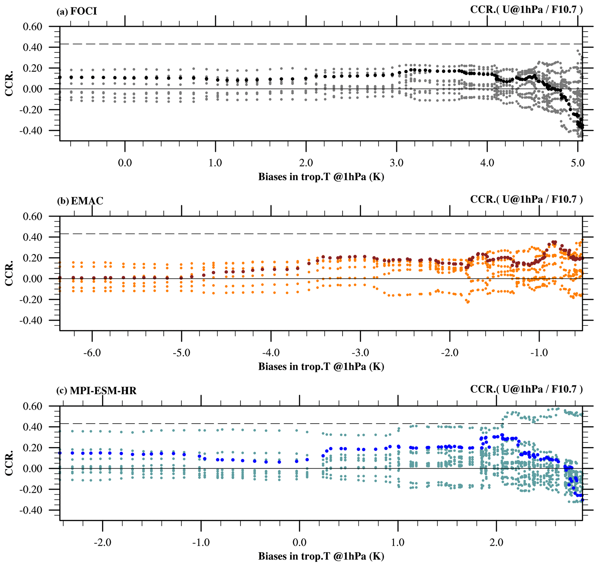
Figure 10 Upper-stratospheric polar night jet responses to solar forcing vs. biases of the tropical stratopause temperature. Scatter plots of correlation coefficients between the December zonal-mean zonal wind anomalies averaged over 60–65° N at 1 hPa and the F_10.7 index vs. biases of the tropical stratopause temperature averaged over 25° S–25° N at 1 hPa in all 45-year windows for (a) FOCI (black: ensemble mean; light gray: individual members), (b) EMAC (brown: ensemble mean; light brown: individual members), and (c) MPI-ESM-HR (blue: ensemble mean; light blue: individual members). The dashed black line indicates the 95 % significance level.

To further explore the possible causes of the model biases in the meridional temperature gradient and their influences on the solar fingerprints in the PNJ anomalies, we show scatter plots of the correlation coefficients between the PNJ anomalies at 1 hPa and the F_10.7 index for all 45-year windows vs. model temperature biases at 1 hPa averaged over the polar box (Fig. 9) and tropical box (Fig. 10). As shown in Fig. 9, all three models have a warm bias in the pole region (65–90° N) compared to the ERA5, which is much larger in MPI-ESM-HR. This warm pole bias in general is the main reason for the weak poleward meridional gradient (ΔT) for all three models. The simulated temperature in the tropical stratopause (i.e., the tropical box at 1 hPa) shows a slight positive bias in FOCI and a negative bias in EMAC (Fig. 10a and b as well as Fig. A8a and b). The negative bias of the tropical stratopause in EMAC is partly responsible for the weak ΔT in this model. Both cold and warm biases of the tropical stratopause appear in MPI-ESM-HR (Fig. 10c). Further examination indicates that the warm bias appearing in the early period (before 1960) could be just an “overestimation” due to the very different climate states of the earlier period from the ERA5 climatology (the figure is not shown here). The positive correlation coefficients of the ensemble mean December PNJ anomalies with the 11-year solar cycle are replaced by negative correlation coefficients in FOCI and MPI-ESM-HR when the warm biases in the tropical box (Fig. 10a and c) reach their maxima. In addition, the positive responses in the ensemble mean PNJ anomalies in all three models are not significant. However, the positive response of the upper-stratospheric PNJ anomalies (1 hPa) in EMAC increases and is more robust when the cold bias in the tropical stratopause decreases (Fig. 10b). No significant (or robust) PNJ responses appear in the middle stratosphere (i.e., at 10 hPa here). The approximately even distribution of the positive and negative correlation coefficients between zonal mean zonal wind anomalies at 10 hPa and the F_10.7 index in FOCI and MPI-ESM-HR suggests the PNJ responses in the middle stratosphere in these two models are not sensitive to the mean flow strength or to the temperature of both the pole and the tropical regions (figures are not shown here). However, a robust positive PNJ response can be found in EMAC, and it is enhanced when the PNJ strength increases (the figure is not shown here).

To summarize, a strengthened PNJ response to the 11-year solar cycle only shows up in the upper stratosphere (1 hPa) in FOCI and MPI-ESM-HR when the warming response in the tropical stratopause is robust and significant. In EMAC, the strengthened PNJ response exists in both the upper and middle stratosphere, which is not sensitive to the magnitude of the solar variability but is influenced by the background states (e.g., wind speed of the mean flow). The cold bias in the tropical stratopause of EMAC likely dampens the initial solar signal, and together with the warm bias in the polar region, they lead to a weak meridional temperature gradient and a weak PNJ in this model. FOCI has a warm bias in both the tropics and the north pole zone of the upper and middle stratosphere, which may be responsible for the sensitivity of the initial solar signals to the magnitude of the solar forcing. However, the PNJ in FOCI being too strong possibly dampens the upward propagation of planetary waves and hence influences the downward propagation of the initial solar signal in the winter season.

4 Conclusions

This study aimed to assess the 11-year solar cycle signal in the middle atmosphere since the detected solar imprints in previous studies still show large discrepancies among different climate models, and the solar signal in a relatively short period with reliable observations is hard to distinguish from other signals or internal variability. For this purpose, two sets of CMIP6 historical-like ensemble simulations – the FULL and the FIX experiments – were performed with two CCMs (i.e., FOCI and EMAC) and one high-top climate model without interactive chemistry (i.e., MPI-ESM-HR). Each set of simulations is forced by identical CMIP6 external forcings and a different solar forcing – full solar variability in FULL and no solar variability in FIX. To avoid any artificial signals, our statistical analysis is mainly based on the FULL ensemble and compared the result with FIX at some points to derive the possible impacts of solar forcing. In addition, the ensemble mean of the FULL simulations can extract the solar signal to some extent.

Our results show a robust and significant solar imprint on the SWHR and temperature anomalies in the upper stratosphere, as well as in the ozone anomalies in the middle stratosphere (in the two CCMs). FOCI simulated stronger 11-year solar cycle signals in the SWHR and temperature anomalies in the upper stratosphere above 4 hPa and a larger ozone response than EMAC. When the solar cycle amplitude, indicated by the standard deviation of the DJF-mean F_10.7 in the 45-year running window, is smaller than 40, the responses of the SWHR, temperature, and ozone anomalies in the tropical upper stratosphere with all three models show linear reliance on the solar cycle amplitude (i.e., their positive correlation coefficients increase along with the solar cycle amplitude). However, the reliance of the detected solar signals in the SWHR, temperature, and ozone anomalies on the strength of solar activity is more complex at SC ≥ 40. The middle-stratospheric temperature response to the 11-year solar cycle simulated by FOCI is sensitive to the solar cycle amplitude, which is not the case for EMAC and MPI-ESM-HR.

Although all three models simulated a warm response in the tropical upper stratosphere to the 11-year solar cycle forcing, the responses in the poleward meridional temperature gradient as well as the zonal-mean zonal wind anomalies are quite different between the models. The top-down mechanism that has been claimed to explain the downward propagation of the initial solar signals transport from the middle atmosphere to the troposphere can be found in the ensemble mean of FULL with FOCI, and the responses are more significant in a strong epoch with large solar cycle amplitude. However, the top-down response in the ensemble mean of FULL is much weaker in MPI-ESM-HR and has no clear downward propagation in EMAC. These diverse results from multiple climate models suggest the 11-year solar cycle signal and its transport in the atmosphere are more complex than expected. The linear methods used in this study (i.e., the ensemble mean and the composite difference between solar maximum and minimum) may not be able to extract the 11-year solar cycle signal from the background noise (e.g., large internal variability in the zonal mean zonal wind in the PNJ region).

Our further analysis with a particular focus on the December PNJ dynamical response suggests that model biases can influence the imprints of the 11-year solar cycle. A strengthened PNJ response (but not significant) to the solar cycle in the upper stratosphere (1 hPa) can be found in all three models when the warming response in the tropical stratopause is robust and significant. No robust December PNJ response can be found in the middle stratosphere (10 hPa) in FOCI and MPI-ESM-HR. However, the simulated PNJ response in EMAC is not sensitive to the solar cycle amplitude but is influenced by the biases of the PNJ strength and tropical stratopause temperature. The warm bias in the pole region and cold bias in the tropical stratopause of EMAC lead to a large negative bias in the meridional temperature gradient, which dampens the initial 11-year solar cycle signal in the tropical upper stratosphere and thereby limits the zonal-mean zonal wind responses in the high latitude and pole region. The large warm pole bias in the middle and upper stratosphere of the MPI-ESM-HR leads to a weak PNJ and may be responsible for the weak dynamical responses in this model. In addition, the zonal wind in the polar vortex region in FOCI being too strong may lead to a reversed (weakened) PNJ response.

Appendix A: Figures A1–A7

Figure A1 The same as Fig. 2 but for the solar-fixed historical simulations (i.e., FIX.)

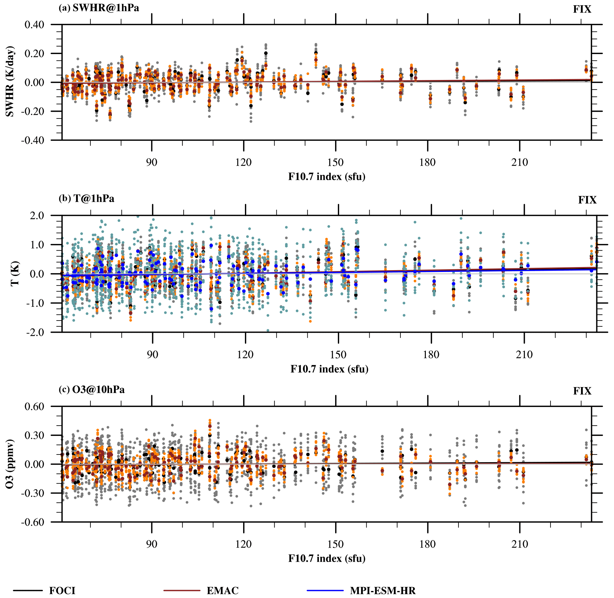
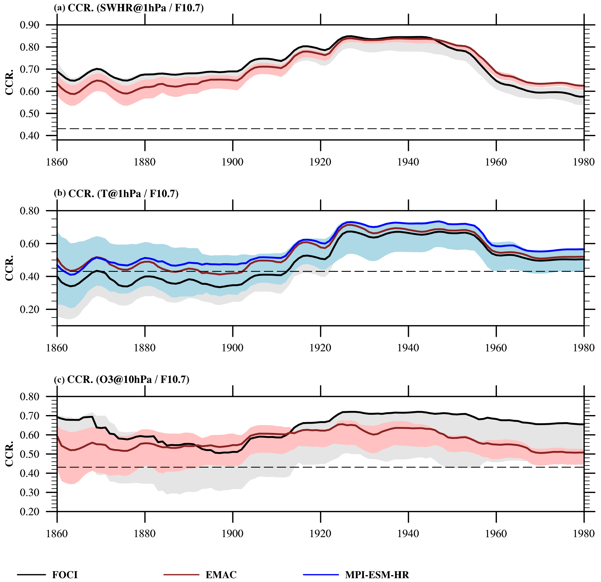
Figure A2 (a) Correlation coefficients between the annual shortwave heating rate in the tropical stratopause (averaged over 25° S–25° N at 1 hPa) and the annual F_10.7 index in a 45-year running window for FOCI (black) and EMAC (brown). Solid lines represent the correlation coefficients of the ensemble mean for each model and the shadow regions indicate the spread of correlation coefficients among individual members (between maximum and minimum). The dashed black line indicates the 95 % significance level. Panel (b) is the same as (a) but for the temperature from FOCI (black), EMAC (brown), and MPI-ESM-HR (blue). Panel (c) is the same as (a) but for the O₃ volume mixing ratio at 10 hPa from FOCI and EMAC.

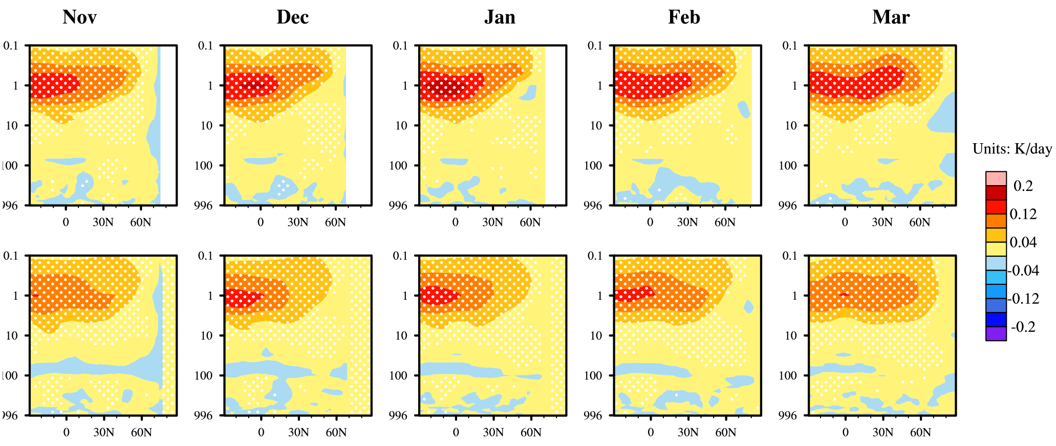
Figure A3 Composite differences between solar maxima and minima of the ensemble mean zonal-mean shortwave heating rate anomalies (units: K d⁻¹; color shading contours) in the FULL experiment with FOCI (top panels) and EMAC (bottom panels). Latitude–height cross sections are from 30° S to 90° N and 996 to 0.1 hPa. The 90 % significance level for the composite of air temperature anomalies is indicated by white dots based on a 1000-fold bootstrapping test.

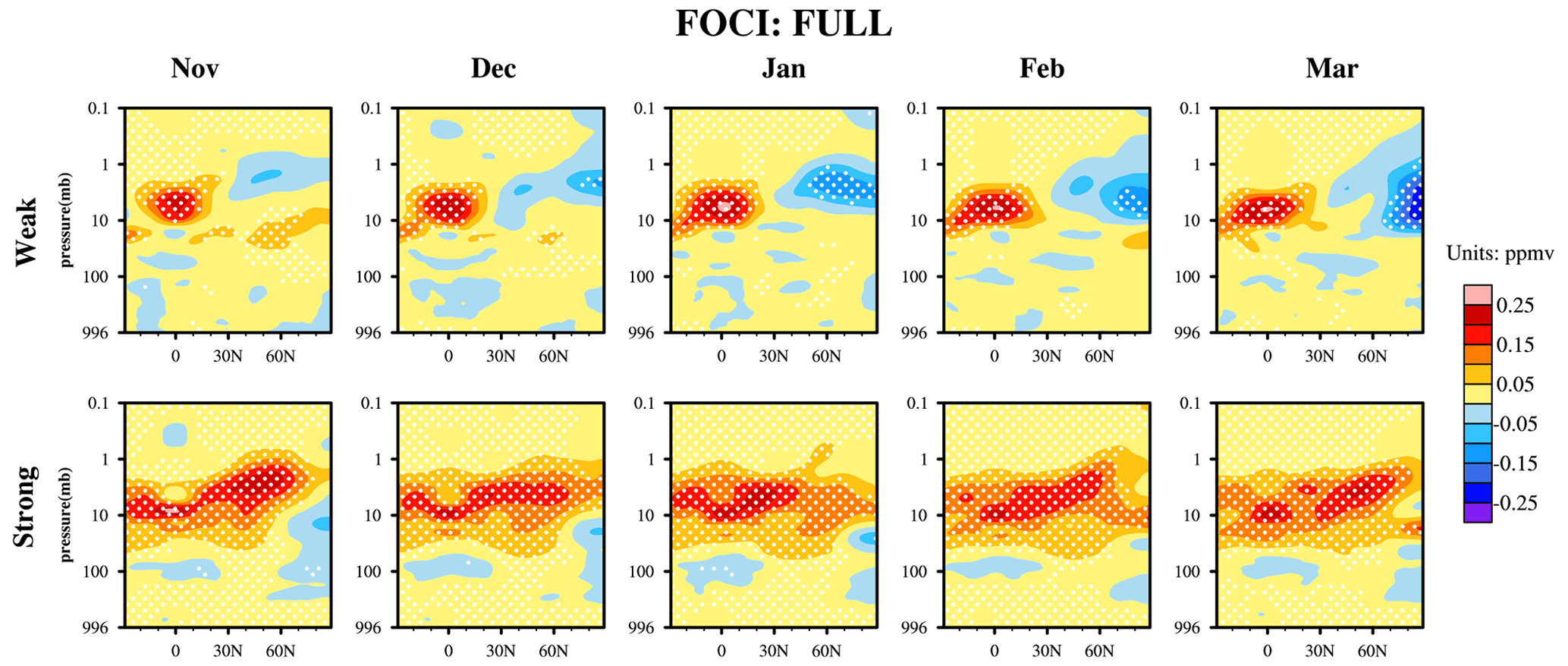
Figure A4 Composite differences between solar maxima and minima of the ensemble mean zonal-mean O₃ volume mixing ratio anomalies (units: ppmv; color shading contours) in the FULL experiment with FOCI during the weak (top panels) and strong solar epochs (bottom panels). Latitude–height cross sections are from 30° S to 90° N and 996 to 0.1 hPa. The 90 % significance level for the composite of air temperature anomalies is indicated by white dots based on a 1000-fold bootstrapping test.

Figure A5 Composite differences between solar maxima and minima of the ensemble mean zonal-mean air temperature anomalies (units: K; color shading contours) and the poleward meridional temperature gradients (units: K (100 km)⁻¹; contours) in the FULL experiment with FOCI during the weak (top panels) and strong solar epochs (bottom panels). Latitude–height cross sections are from 30° S to 90° N and 996 to 0.1 hPa. Only the positive meridional temperature gradient anomalies (poleward) are shown here. The 90 % significance level for the composite of air temperature (meridional gradients) anomalies is indicated by white dots (black hatching) based on a 1000-fold bootstrapping test.

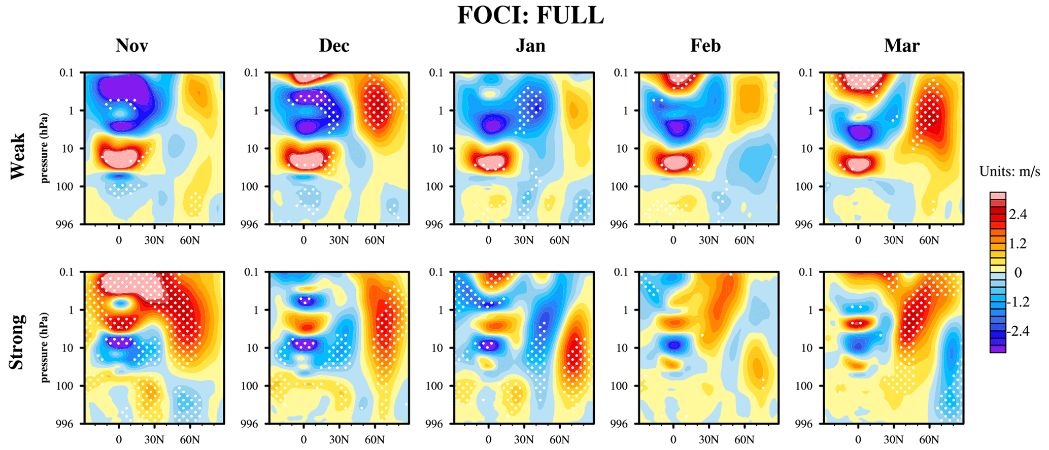
Figure A6 Composite differences between solar maxima and minima of the ensemble mean zonal-mean zonal wind anomalies (units: m s⁻¹; color shading contours) in the FULL experiment with FOCI during the weak (top panels) and strong solar epochs (bottom panels). Latitude–height cross sections are from 30° S to 90° N and 996 to 0.1 hPa. The 90 % significance level for the composite of zonal-mean zonal wind anomalies is indicated by white dots (black hatching) based on a 1000-fold bootstrapping test.

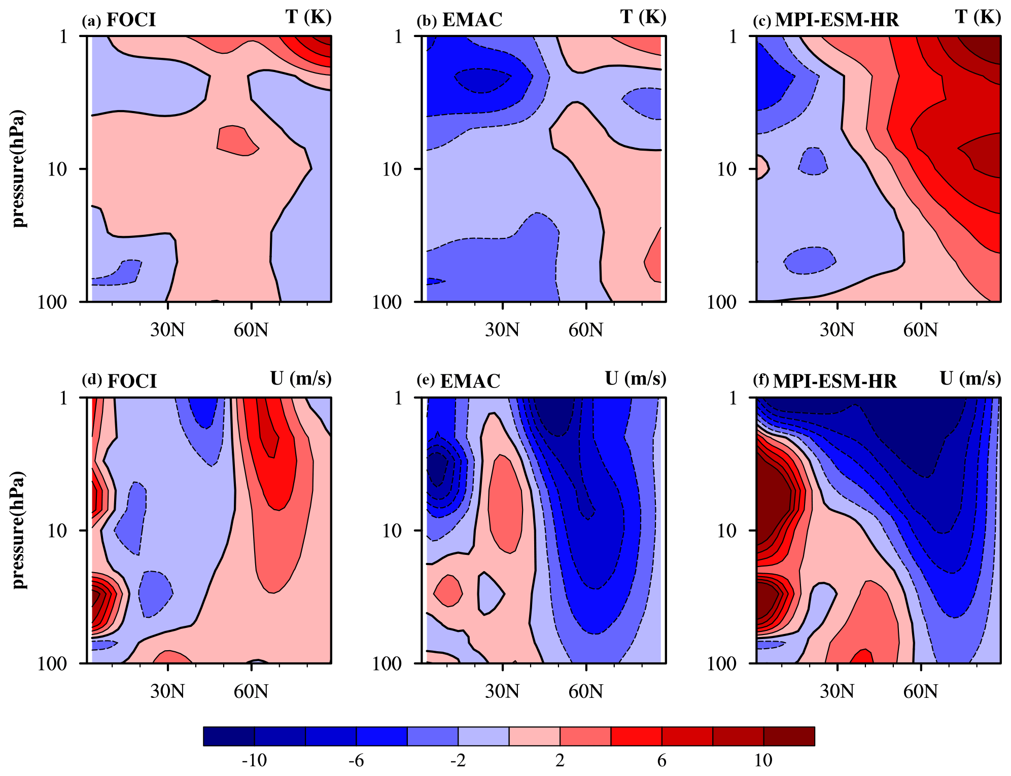
Figure A7 (a–c) Differences in the zonal mean temperature climatology (K) between models ((a) FOCI, (b) EMAC, and (c) MPI-ESM-HR) and ERA5. (d–f) The same as the first row but for the zonal mean zonal wind climatology (m s⁻¹). Here, the climatology is defined by the mean value of 1950–2014 for all models and the ERA5.