Multi-model assessment of the atmospheric and radiative effects of supersonic transport aircraft

Commercial supersonic aircraft may return in the near future, offering reduced travel time while flying higher in the atmosphere than subsonic aircraft, thus displacing part of the passenger traffic and associated emissions to higher altitudes. For the first time since 2007, we present a comprehensive multi-model assessment of the atmospheric and radiative effect of this displacement. We use four models (EMAC, GEOS-Chem, LMDz–INCA, and MOZART-3) to evaluate three scenarios in which subsonic aviation is partially replaced with supersonic aircraft. Replacing 4 % of subsonic traffic with Mach 2 aircraft that have a NO_x emissions index of 13.8 g (NO₂) kg⁻¹ leads to ozone column loss of −0.3 % (−0.9 DU; model range from −0.4 % to −0.1 %), and it increases radiative forcing by 19.1 mW m⁻² (model range from 16.7 to 28.1). This forcing is driven by water vapor (18.2 mW m⁻²), ozone (11.4 mW m⁻²), and aerosol emissions (−10.5 mW m⁻²). The use of a Mach 2 concept with low-NO_x emissions (4.6 g (NO₂) kg⁻¹) reduces the effect on forcing and ozone to 13.4 mW m⁻² (model range from 2.4 to 23.4) and −0.1 % (−0.3 DU; model range from −0.2 % to +0.0 %), respectively. If a Mach 1.6 aircraft with a lower cruise altitude and NO_x emissions of 4.6 g (NO₂) kg⁻¹ is used instead, we find a near-net-zero effect on the ozone column and an increase in the radiative forcing of 3.7 mW m⁻² (model range from 0.5 to 7.1). The supersonic concepts have up to 185 % greater radiative effect per passenger kilometer from non-CO₂ emissions compared to subsonic aviation (excluding contrail impacts).

1 Introduction

Over the past few decades, there has been growing global demand for fast intercontinental transportation. This demand has led to a search for faster alternatives to subsonic aircraft, such as supersonic or even hypersonic vehicles (Kinnison et al., 2020; Pletzer et al., 2022; Matthes et al., 2022; Eastham et al., 2022). Supersonic transport (SST) aircraft have already attracted considerable commercial interest, and several parties are working towards the reintroduction of civil supersonic transportation, relying on new technologies such as low-boom hull designs to minimize the environmental effect of the sonic boom (Berton et al., 2020). An example of this development is NASA's X-59 demonstrator aircraft, which has recently gone through engine testing and is planned to have its first flight in 2025.

SSTs generally use higher cruise altitudes, ranging from 14 to 21 km, compared to subsonic aircraft which typically cruise between 9 and 12 km. The increase in operational altitude changes the atmospheric response to the aircraft's emissions. Of particular concern are the emissions of nitrogen oxides (NO_x), water vapor (H₂O), and sulfur compounds that affect the distribution and chemistry of ozone (O₃) and global radiative forcing (RF). NO_x and H₂O emissions from SSTs lead to the catalytic destruction of ozone through the NO_x and HO_x cycles (Matthes et al., 2022; Grewe et al., 2007; Solomon, 1999; Crutzen, 1972; Johnston, 1971), while sulfur emissions lead to the formation of sulfate aerosols (SO₄) that facilitate ozone destruction through heterogeneous chemistry (Pitari et al., 2014; Granier and Brasseur, 1992). Through these emissions, the adoption of SSTs has been previously been linked to large-scale changes in the ozone distribution, with higher-emission altitudes being linked to the increased depletion of the global ozone column (van 't Hoff et al., 2024; Fritz et al., 2022; Zhang et al., 2021a; Speth et al., 2021). This is associated with a risk to public health, as the subsequent increase in surface UV exposure affects mortality (Eastham et al., 2018b). Additionally, several studies have identified the changes in the ozone distribution as the primary warming driver of the radiative effect of non-CO₂ emissions from supersonic aircraft (van 't Hoff et al., 2024; Zhang et al., 2023; Eastham et al., 2022), although others have also found this to have a net cooling effect instead (Zhang et al., 2021b; Grewe et al., 2007).

Other non-CO₂ emissions that affect RF are water vapor and aerosols (black carbon and sulfate). Water vapor directly affects RF, and it plays a pivotal role in the climate effect of subsonic aviation through the formation of contrails (Lee et al., 2021). At supersonic cruise altitudes, contrail formation is expected to be much less common due to the drier conditions in the stratosphere (Stenke et al., 2008; Grewe et al., 2007; IPCC, 1999); however, the water vapor perturbation lifetime is longer compared to at subsonic altitudes. Grewe and Stenke (2008) estimate that this lifetime is up to around 1.5 years at 20 km altitude, compared to lifetimes of 1 to 6 months at subsonic cruise altitudes. This facilitates more accumulation of stratospheric water vapor, which has a direct warming effect. The emission of water vapor has also been identified as a critical, if not the primary, driver of radiative forcing from SSTs and hypersonic vehicles (Pletzer and Grewe, 2024; Pletzer et al., 2022; Zhang et al., 2021a; Grewe et al., 2010, 2007). The stratospheric accumulation of aerosols also affects RF, but they are commonly associated with a cooling effect instead (van 't Hoff et al., 2024; Zhang et al., 2023; Eastham et al., 2022; Speth et al., 2021). Combined, most studies find that the adoption of supersonic aircraft leads to warming RF (van 't Hoff et al., 2024; Zhang et al., 2023, 2021a; Eastham et al., 2022; Speth et al., 2021; Grewe et al., 2007).

The ozone and climate effects stem from changes in the chemical composition of the atmosphere, particularly the stratosphere. To adequately capture these changes, we rely on chemistry transport models (CTMs) or chemistry climate models (CCMs), which model the chemistry, transport, removal, and conversion of species throughout the atmosphere. A variety of these models has already been used to evaluate the effects of high-altitude emissions on ozone and RF, and despite their similar scope and chemistry routines, these models often yield different results. These differences are partially driven by uncertainties about the future of supersonic civil aviation, resulting in the use of different emission scenarios and timelines across studies. However, multi-model studies also highlight that there are considerable differences between different CTMs and CCMs, even in the evaluation of identical scenarios. Model differences have been reported in studies of supersonic (Pitari et al., 2008; Grewe et al., 2007; Kawa et al., 1999) and subsonic aviation (Olsen et al., 2013). These differences are most prevalent in the evaluation of the ozone response, which is subject to complex feedback mechanisms. Differences in the modeling thereof can result in a large spread in model predictions of the ozone response and its effect on RF, at times leading to contradictory results between models (e.g., Grewe et al., 2007; Kawa et al., 1999). The effect of these differences is also evident when metrics such as sensitivities to specific emission species are compared between studies and models (van 't Hoff et al., 2024; Eastham et al., 2022).

The differences in the model responses to SST emissions are often driven by different implementations of chemical, transport, or radiative processes across the models or by differences in interactions between these model components. They are also affected by fundamental properties, such as the model resolution. Understanding the effect of model-driven differences is vital to our capability to synthesize results across studies that use different models. Multi-model studies expose these differences and can help us understand their drivers, potentially offering robust conclusions and policy advice. In the field of SST emissions, the most recent multi-model study performed was by Grewe et al. (2007). They showed that the four atmospheric models they used agreed that the introduction of SST emissions led to net depletion of ozone, accumulation of stratospheric water vapor, and a net warming radiative effect. However, they also showed that there was a spread in the calculations of these effects in terms of the spatial distribution and in absolute numbers. For example, they report a model mean ozone perturbation of −8 Tg with a model range from −16 to −1 Tg and a standard deviation of 5.5 Tg. Before that, Kawa et al. (1999) used seven different models to study the effect of SST emissions, reporting a similar spread in model calculations (e.g., they report a mean ozone column loss of −0.17 % with a model range from −0.6 % to 0.23 % and a standard deviation of 0.22 %; HSR scenario 4). In both cases, the standard deviation of the model predictions is similar to the mean, highlighting the magnitude of model-driven differences.

Over the past few decades, there have been considerable advances in our understanding of the underlying chemistry and physics, and at the same time, the increased availability of computational power has expanded our capacity to model these processes. This has led to enhancements in the overall modeling capabilities of CTMs and CCMs. To assess the effect of these developments, Zhang et al. (2021a) have compared the WACCM6 model to models used by Kawa et al. (1999) in a reassessment of their scenarios, finding similar overall atmospheric effects despite the higher fidelity in their model. While this does provide some insight with respect to older evaluations, it remains unclear how the past 2 decades of model development affect model-driven differences in assessments of an identical scenario. Understanding these differences can help us better synthesize results from studies that use different models.

To close this gap, we present a comprehensive study of the effect of the partial replacement of subsonic traffic with SSTs on atmospheric composition and RF, using four widely used chemistry climate and chemistry transport models (EMAC, GEOS-Chem, LMDz–INCA, and MOZART-3). We evaluate three SST adoption scenarios based on the scenarios considered by Grewe et al. (2007) that reflect the partial replacement of subsonic traffic with different supersonic aircraft concepts or emission characteristics. We also analyze differences in atmospheric responses between the models. In particular, we cover the responses of water vapor, NO_x, ozone, odd oxygen loss rates, and RF, as well as how these differ between the models. The output of these models is presented in a harmonized way in order to provide a comprehensive and multi-model overview of the atmospheric and radiative effects of the adoption of supersonic aircraft.

2 Emission scenarios

Our emission scenarios are based on emission scenarios from the SCENIC project (Grewe and Stenke, 2008; Grewe et al., 2007). The SCENIC emission scenarios consider the adoption of a fleet of SSTs in 2050, replacing part of the revenue passenger kilometers (RPKs) of subsonic aviation. We consider a baseline scenario (S0) with only subsonic aviation emissions (S4 from Grewe et al., 2007). The nominal supersonic scenario (S1) considers the replacement of 4 % of subsonic RPKs with a fleet of 501 SSTs operating at Mach 2.0 with cruise altitudes from 16.5 to 19.6 km (S5 of Grewe et al., 2007). This results in an increase of 6.3 % in global aviation fuel consumption. The triple-NO_x scenario (S2) is a variant of the nominal scenario (S1) with tripled supersonic NO_x emissions, resulting in a fleet-averaged emission index of 13.80 kg (NO₂) kg⁻¹ for the SSTs. This is closer to the NO_x emission indices from recent SST concepts (Zhang et al., 2023, 2021a; Fritz et al., 2022; Eastham et al., 2022; Speth et al., 2021). In the low-cruise scenario (S3), we consider the use of a SST with a lower cruise altitude from 13.1 to 16.7 km and a cruise speed of Mach 1.6 (P6 from Grewe et al., 2007). Compared to the nominal emissions, this leads to a 5.5 % reduction in supersonic RPKs and a 31 % reduction in SST fuel consumption. The characteristics of the emission scenarios are summarized in Table 1, and the resulting changes in the distribution of aviation emissions are shown in Fig. 1.

Table 1 Summary of the sub- and supersonic aircraft emissions in the SST scenarios. The baseline scenario (S0) has no supersonic aviation, and there are three scenarios considering the partial replacement of subsonic aviation with supersonic aircraft. These are denoted as the nominal supersonic scenario (S1), a triple-NO_x scenario (S2), and the low-cruise scenario (S3). In all of the supersonic scenarios, subsonic traffic is partially replaced by the supersonic aircraft, reducing the fuel consumption of subsonic aircraft compared to the baseline. Within each category, the left (Sub.) column summarizes the subsonic aircraft emissions, and the right (Sup.) column summarizes the supersonic aircraft emissions.

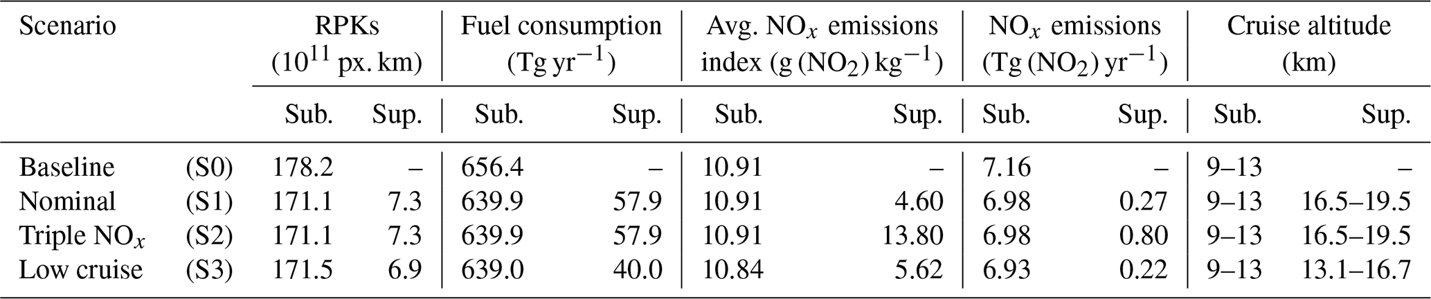
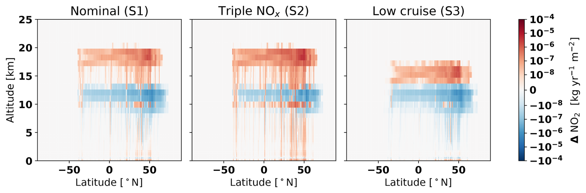
Figure 1 Zonal mean changes in the distribution of annual NO_x emissions (expressed in kg (NO₂) m⁻² yr⁻¹) due to the partial replacement of subsonic traffic with SSTs. Differences are calculated with respect to the annual baseline (S0) emissions.

3 Atmospheric modeling

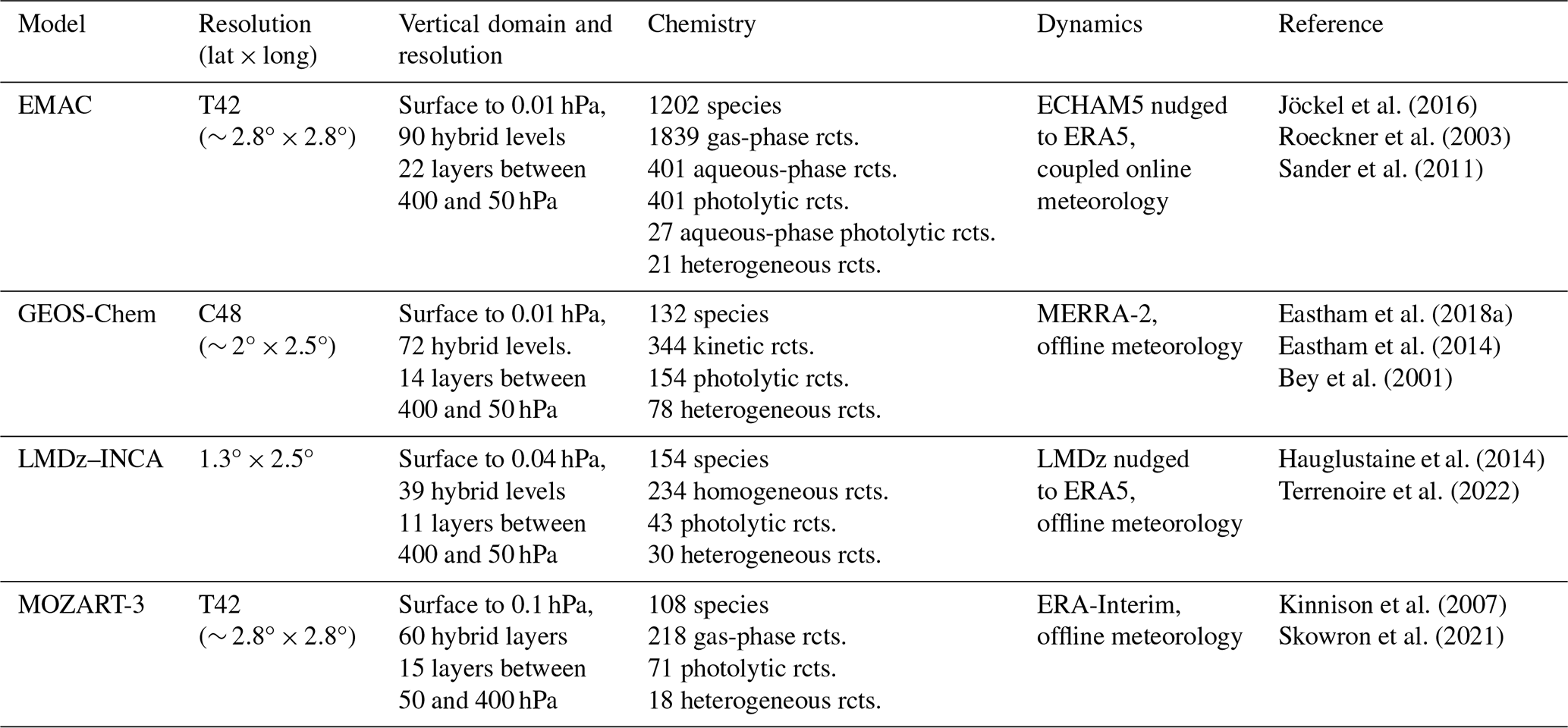
We evaluate the effect of the changes in aviation emissions on atmospheric composition and radiative forcing using four widely used chemistry transport models, namely EMAC, GEOS-Chem, LMDz–INCA, and MOZART-3. Key characteristics of these models, including the horizontal and vertical resolution, chemistry processes, and dynamics, are summarized in Table 2. A direct comparison of the vertical grid of the models is also shown in Fig. A1. We evaluate the effect of the SST adoption on a future atmosphere based on projections of the atmospheric composition and anthropogenic emissions in 2050, although there are some differences with respect to how this is incorporated in the different models, given model input availability and other technical restrictions. The next subsections discuss the technical details and setup of each model individually.

Table 2 Summary of the atmospheric models' characteristics, including the resolution, chemistry, and dynamics. Note that rcts. stands for reactions.

3.1 EMAC

EMAC is an atmospheric chemistry general circulation model consisting of the dynamical core ECHAM5 (European Centre HAMburg general circulation model, version 5; Roeckner et al., 2006) and MESSy (Modular Earth Submodel System; Jöckel et al., 2016). The chemical mechanism incorporates the 1839 gas-phase and 21 heterogeneous-phase reactions between 1202 species, which include type 1ab and type 2 polar stratospheric cloud (PSC) processes (Kirner et al., 2011; Jöckel et al., 2010). The reaction rates are from the most recent Jet Propulsion Laboratory evaluation, number 19 (Burkholder et al., 2019). Aerosol background concentrations of sulfates are provided for heterogeneous chemistry using inventories prepared for the chemistry climate model initiative (Jöckel et al., 2016; Gottschaldt et al., 2013). Water vapor is accounted for as specific humidity, which is influenced by gas-, solid-, and liquid-phase processes at all altitudes. It is produced through 55 reactions and destroyed through 6 reactions, and it is affected by physical processes such as rain-out and sedimentation. The radiation scheme incorporates 81 bands and recreates the solar cycle with high fidelity. This applies to the region from the top of the model domain (0.01 hPa) to 70 hPa (Kunze et al., 2014; Dietmüller et al., 2016). RF is assessed at the tropopause with the radiative code of ECHAM5 (Roeckner et al., 2006), as well as a new radiative code based on the work by Pincus and Stevens (2013), as implemented by Nützel et al. (2024).

In this work, we use EMAC version 2.55.2 (The MESSy Consortium, 2021) with a T42 global grid (approximately 2.8° × 2.8° latitude, longitude) and 90 hybrid vertical levels from the surface up to 80 km. In total, 22 of these layers are located between 400 and 50 hPa, with an average thickness of 0.6 km. The model has online meteorology that is nudged towards ERA5 reanalysis data (2000–2010) between the surface and 10 hPa. Nudging is applied in the same way as earlier studies (Pletzer et al., 2022; Jöckel et al., 2016), affecting horizontal and vertical winds, temperature (wave 0 omitted), and the logarithm of surface pressure. The background atmosphere, surface boundary conditions, and non-aviation anthropogenic emissions are based on the CMIP6 SSP3-7.0 scenario for the year 2050 (Meinshausen et al., 2020). Volcanic emissions are included based on the AeroCom emission inventory (Dentener et al., 2006; Ganzeveld et al., 2006) for the year 2000, which is cycled throughout the model run. We also apply a spin-up method to reduce spin-up times, while maintaining annual quasi-equilibrium. This is done by applying an altitude-dependent scaling factor to the emissions during the first year of the model run so that the annual quasi-equilibrium is achieved faster. For more details on this method, we refer to the work by Pletzer and Grewe (2024) and its supplement. The model is run for a total of 16 years to allow for a longer analysis period and better statistical significance of the results.

3.2 GEOS-Chem

GEOS-Chem is a community-developed tropospheric–stratospheric CTM with over 280 chemical species based on the Goddard Earth Observing System (GEOS) (Bey et al., 2001). The model uses KPP for kinetic chemistry (Damian et al., 2002) and Fast-JX for photolytic reactions (Bian and Prather, 2002), incorporating stratospheric chemistry through the unified tropospheric–stratospheric chemistry extension (UCX) by Eastham et al. (2014). Within the troposphere, water vapor mixing ratios are prescribed by meteorology, and in the stratosphere the water vapor tracer evolves freely, subject to gas-phase chemistry, photochemistry, and transport. GEOS-Chem's capability to model stratospheric chemistry has been demonstrated against satellite observations in several studies (Fritz et al., 2022; Speth et al., 2021; Eastham et al., 2014), and it is incorporated into NASA's Global Modeling and Assimilation Office (GMAO) GEOS chemical composition forecast (GEOS-CF) (Keller et al., 2021). The model simulates the distribution of various aerosols from anthropogenic and natural sources, and it models heterogeneous reactions in the tropo- and stratospheric domain, including the formation, sedimentation, and evaporation of PSCs (Eastham et al., 2014). RF is evaluated at the tropopause in the same manner as described in van 't Hoff et al. (2024), incorporating a stratospheric adjustment following the implementation by Eastham et al. (2022).

We use version 14.1.1 of the GEOS-Chem High Performance (GCHP) model (The International GEOS-Chem User Community, 2023) with a C48 cubed-sphere global grid (approximately 2° × 2.5° latitude, longitude) and 72 non-uniform vertical levels. The vertical grid has 14 layers between 400 and 50 hPa, with an average thickness of 0.9 km. We use historical meteorological data for the years 2000 to 2010 from the MERRA-2 reanalysis product by NASA/GMAO (Gelaro et al., 2017). Volcanic emissions are incorporated through historical emissions for the same time period, following work by Carn et al. (2015). Surface emissions and mixing ratios of long-lived species are prescribed following the 2050 boundary conditions of the SSP3-7.0 scenario. Simulations are run for a total of 10 years using the same spin-up method as EMAC, which is detailed in Pletzer and Grewe (2024).

3.3 LMDz–INCA

The LMDz–INCA global chemistry–aerosol–climate model couples the LMDz (Laboratoire de Météorologie Dynamique, version 6) general circulation model (GCM; Hourdin et al., 2020) and the INCA (INteraction with Chemistry and Aerosols, version 6) model (Hauglustaine et al., 2014, 2004). LMDz–INCA is part of the Institute Pierre-Simon Laplace (IPSL) coupled model, and we use the “standard physics” parameterization of the GCM (Boucher et al., 2020). The large-scale advection of tracers is calculated based on a monotonic finite-volume second-order scheme (Van Leer, 1977; Hourdin and Armengaud, 1999). Deep convection is parameterized according to the scheme of Emanuel (1991). The turbulent mixing in the planetary boundary layer is based on a local second-order closure formalism. INCA includes state-of-the-art CH₄–NO_x–CO–NMHC–O₃ tropospheric photochemistry (Folberth et al., 2006; Hauglustaine et al., 2004), as well as interactive chemistry in the stratosphere and mesosphere (Terrenoire et al., 2022). The INCA model simulates the distribution of aerosols with anthropogenic sources such as sulfates, nitrates, black carbon (BC), and organic carbon, as well as natural aerosols such as sea salt and dust. Both of the natural and anthropogenic tropospheric aerosols facilitate heterogeneous reactions (Hauglustaine et al., 2014, 2004). Heterogeneous processes on PSCs and stratospheric aerosols are parameterized following the scheme implemented in Lefèvre et al. (1994). INCA incorporates a water vapor tracer that is linked to the LMDz GCM. Similar to GEOS-Chem, this tracer is prescribed by LMDz below the tropopause, and it evolves freely in the stratosphere, subject to chemistry (gas phase and photochemical), transport, condensation, sedimentation, and stratospheric emissions. RF is evaluated using an improved version of the ECMWF scheme developed by Fouquart and Bonnel (1980) in the solar part of the spectrum and by Morcrette (1991) in the thermal infrared. Aerosol forcing is assessed at the top of the atmosphere, similar to Hauglustaine et al. (2014), and forcing from ozone and water vapor is calculated at the tropopause with an offline version of the LMDz GCM with a stratospheric adjustment, similar to Terrenoire et al. (2022).

We use a configuration with a horizontal resolution of 1.3° × 2.5° in latitude and longitude with 39 hybrid vertical levels extending up to 70 km. In total, 11 of these layers are located between 300 and 50 hPa, with an average thickness of 1.1 km. The model is run for 15 years, with initial conditions representative of the year 2050 (Pletzer et al., 2022). Surface emissions and boundary conditions for 2050 are prescribed by the CMIP6 SSP3-7.0 scenario (Meinshausen et al., 2020). Stratospheric volcanic aerosols are based on historical data (2000–2014) from Input4MIP for the calculation of heterogeneous chemistry. In this study, the LMDz GCM zonal and meridional wind components are nudged towards the meteorological data from the European Centre for Medium-Range Weather Forecasts (ECMWF) ERA-Interim reanalysis, with a relaxation time of 3.6 h (Hauglustaine et al., 2004). The ECMWF fields are provided every 6 h and interpolated onto the GCM grid for the years 2004–2018.

3.4 MOZART-3

The Model for OZone And Related chemical Tracers, version 3 (MOZART-3), is an offline CTM (Kinnison et al., 2007) that has been used for an extensive range of applications, including various aspects of the effect of aircraft NO_x emissions on atmospheric composition (e.g., Skowron et al., 2021, 2015, 2013; Freeman et al., 2018; Søvde et al., 2014; Flemming et al., 2011; Liu et al., 2009). MOZART-3 accounts for advection based on a flux form semi-Lagrangian scheme, shallow- and mid-level-convective and deep-convective routines, boundary layer exchanges, and wet and dry deposition. MOZART-3 reproduces detailed chemical and physical processes from the troposphere through the stratosphere, including gas-phase, photolytic, and heterogeneous reactions. The latter includes four aerosol types, namely liquid binary sulfate, supercooled ternary solution, nitric acid trihydrate, and water ice. Heterogeneous processes occurring on liquid sulfate aerosols and PSCs are also included, following the approach of Considine et al. (2000). The kinetic and photochemical data are based on the NASA Jet Propulsion Laboratory (JPL) evaluation (Sander et al., 2006). Water vapor tracers have been implemented into the model for the purpose of this work, allowing water vapor to evolve freely in the stratosphere, subject to transport and chemistry. We assess RF at the tropopause using the SOCRATES model of the UK Met Office (Manners et al., 2015).

We use a model configuration with a T42 (∼ 2.8° × 2.8°) horizontal resolution and 60 hybrid layers from the surface to 0.1 hPa. The vertical grid has 15 layers between 400 and 50 hPa, with an average thickness of 0.8 km. The transport of chemical compounds is driven by 6-hourly reanalysis ERA-Interim data for the year 2006 from the European Centre for Medium-Range Weather Forecasts (ECMWF). The 2050 gridded surface emissions (anthropogenic and biomass burning) are prescribed by integrated assessment models (IAMs) for the business-as-usual scenario of the Representative Concentration Pathways (RCP 4.5). The surface boundary conditions for long-lived species are set to fixed-volume mixing ratio units, with their concentrations determined using the methodology of Meinshausen et al. (2011). This future scenario does not include natural emissions, such as isoprene, NO_x from lightning and soil, or oceanic emissions of CO. The model is integrated for 8 years until a steady state is reached, and the last year of these simulations is considered for the analysis. The assessment of the water vapor perturbation is performed using separate model runs, the output of which has a limited vertical resolution with 30 layers from 200 to 0.1 hPa.

3.5 Approach for evaluating atmospheric and radiative effects

We quantify the effect of the SST emissions by comparing the perturbed atmospheric composition and forcing of the supersonic scenarios with that of the baseline simulation, thereby also taking into account the effects of the reduction in subsonic emissions. For example, results presented as the effect of the nominal SST fleet (scenario S1) show changes in atmospheric composition and RF calculated by subtracting the baseline atmosphere from the nominal scenario atmosphere, thereby isolating changes from the replacement of subsonic RPKs with the nominal SST. To account for inter-annual variability, we calculate the effect of the emissions over the last 3 years of the model integrations for GEOS-Chem and LMDz–INCA. For EMAC, we average over 6 years to improve the statistical significance of the results, considering the added variability from its online meteorology. For MOZART-3, we show an annual average considering its cycling meteorology. We calculate the stratospheric perturbation lifetime (e-folding lifetime) of emission species by dividing the stabilized stratospheric perturbation by the increase in annual stratospheric emissions. Since not all models calculate forcing from aerosol perturbations, we first calculate model mean RF from ozone, water vapor, and aerosols separately, the results of which are then combined to produce a first-order estimate of the net radiative effect.

4 Results

We present a comprehensive review of the effects of the partial replacement of subsonic traffic with SSTs on atmospheric composition and RF using four atmospheric chemistry transport models for the first time since the work by Grewe et al. (2007). In Sect. 4.1, we summarize the model mean (mean over all models) effect of the adoption of the SST fleets on the atmospheric composition and RF, and we compare the models' baseline atmospheres. Section 4.2 to 4.6 discuss in more detail how the supersonic scenarios affect stratospheric water vapor, nitrogen oxides, ozone, odd oxygen (O_x) loss rates, and RF, respectively. In these sections, we also explore the differences between the models we use.

4.1 Global atmospheric and radiative effect

Table 3 provides a summary of the key variables representing the changes in atmospheric composition and RF in response to the supersonic scenarios across all models. Comprehensive tables of the effects on water vapor, NO_x, and ozone, are included in the Appendix (Tables A1 to A3). Similar to Grewe et al. (2007), we include the hemispheric ratio, which is the ratio of the perturbation mass in the Northern Hemisphere over the perturbation mass in the Southern Hemisphere, as a means to quantify the mixing of emissions between hemispheres. For reference, the hemispheric ratio for the SST fuel consumption is 10.14 for the nominal and triple-NO_x scenarios and 10.34 for the low-cruise scenario, indicating that the vast majority of SST emissions take place in the Northern Hemisphere.

Table 3 Summary of the effects on stratospheric water vapor, stratospheric NO_x, ozone column, and RF for the SST scenarios. These values are calculated as the differences between the perturbed and baseline atmospheres. For more extensive summaries of the effects on H₂O, NO_x, and O₃, including background mass budgets, see Tables A1–A3 in the Appendix. The inorg. aer. (inorganic aerosol) column contains the RF from changes in nitrates and sulfates.

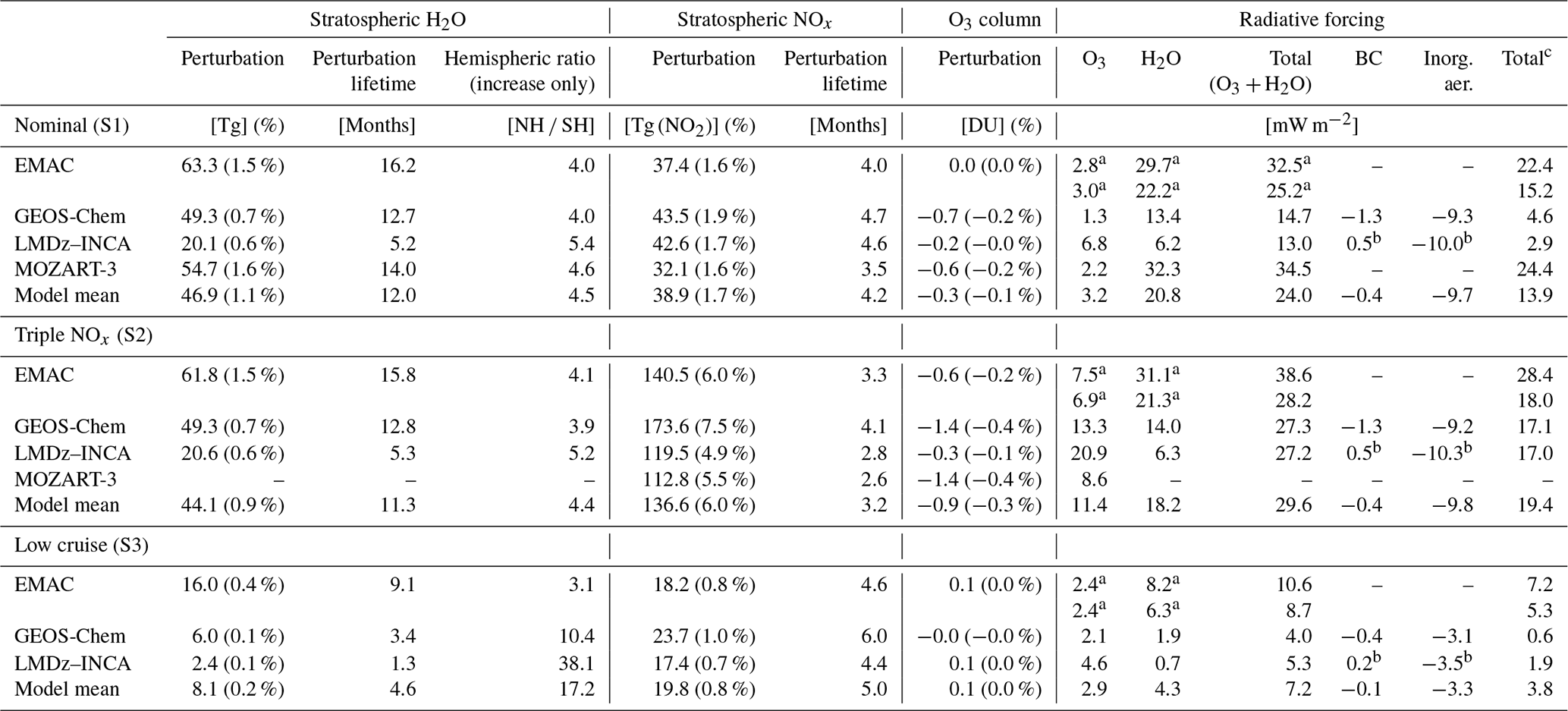
^a For EMAC, two numbers are shown for the RF assessment; the upper value is calculated using the ECHAM5 radiative scheme and the lower value with the scheme by Pincus and Stevens (2013). Both are considered in the mean.
^b These aerosol forcings are calculated at the top of the atmosphere. ^c Total forcing with aerosols is calculated with the model mean aerosol forcings.

In response to the nominal supersonic scenario (S1), we find a model mean stratospheric water vapor perturbation of 46.9 Tg (model range from 20.1 to 63.3 Tg) with a lifetime of 12.0 months (model range from 5.2 to 16.2). The change in aviation emissions leads to increases in stratospheric NO_x, with a model mean perturbation of 38.9 Gg (NO₂) (model range from 32.1 to 43.5), and global ozone column changes of −0.1 % (−0.3 DU; model range from −0.2 % (−0.7 DU) to (0.0 % (0.0 DU)). RF is also affected, with the largest forcing being from water vapor (20.8 mW m⁻²; model range from 6.2 to 32.3), followed by ozone (3.2 mW m⁻²; model range from 1.3 to 6.8). Increases in stratospheric aerosols have a cooling effect, with a forcing of −0.4 mW m⁻² from black carbon and −9.7 mW m⁻² from inorganic aerosols (sulfates and nitrates). We therefore estimate a model mean net RF of 13.9 mW m⁻² when aerosols are included (model range from 2.9 to 24.4).

In the case of the triple-NO_x scenario (S2), the stratospheric NO_x accumulation increases by a factor of 3.5 to a model mean of 136.6 Gg (NO₂) (model range from 112.8 to 173.6). In this case, the model mean water vapor perturbation is 44.1 Tg (model range from 20.6 to 61.8), and the model mean ozone column depletion increases to −0.3 % (−0.9 DU; model range from −0.4 % (−1.4 DU) to −0.1 % (−0.3 DU)). RF from ozone is also enhanced, increasing to 11.4 mW m⁻² (model range from 6.9 to 20.9), but RF from water vapor is still dominant, with a mean value of 18.2 mW m⁻² (model range from 6.3 to 31.1). We find RF of −0.4 mW m⁻² from black carbon and −9.8 mW m⁻² from inorganic aerosols. Including these, the estimated model mean net RF is 19.4 mW m⁻² (model range from 17.0 to 28.4).

When the supersonic cruise altitude and speed are reduced (scenario S3), the effects of the SST adoption on the atmospheric composition and RF are reduced as well. Scenario S3 has 30 % less SST fuel burn compared to the nominal scenario (S1), but the reduction in atmospheric and radiative effects exceeds that. In this case, we find a model mean water vapor perturbation of 8.1 Tg (model range from 2.4 to 16.0) with a lifetime of 4.6 months (model range from 1.3 to 9.1). The stratospheric NO_x perturbation is reduced to a model mean of 19.8 Gg (NO₂) (model range from 17.4 to 23.7), and the ozone column does not change significantly (model mean of 0.0 %, model range of 0.0 to 0.1 DU). The accumulation of stratospheric water vapor still has the largest contribution to radiative forcing (4.3 mW m⁻²; model range from 0.7 to 8.2), followed by cooling from aerosols (−0.1 mW m⁻² from black carbon and -3.3 mW m⁻² from inorganic aerosols) and ozone (2.9 mW m⁻², 0.7 to 4.6). The estimated total forcing is 3.8 mW m⁻² (range 0.6 to 7.2).

Despite some differences in the model configurations and inventories, we find that the models have similar budgets of water vapor, NO_x, ozone, and halogens in their baseline atmospheres (Tables A1 to A4). The GEOS-Chem model stands out as having more stratospheric water vapor than the other models. Furthermore, the MOZART-3 baseline atmosphere has around 15 % less stratospheric NO_x compared to the other models. This may be related to the use of the RCP 4.5 boundary conditions rather than SSP3-7.0 (Meinshausen et al., 2020) and also to the use of ECMWF reanalysis meteorology, as this has been reported to lead to underestimations of stratospheric NO_x mixing ratios before with the MOZART-3 model (Kinnison et al., 2007). The effects of the differences in baselines on the response to the SST emissions are discussed further in the relevant sections.

4.2 Water vapor

Figure 2 shows the zonal average water vapor perturbations from the nominal supersonic scenario (S1) as evaluated by the four models. The vertical averages for all three scenarios are shown in Fig. A2. We find that the perturbation patterns of stratospheric water vapor agree across the models. The strongest increases, in terms of mixing ratios, occur around the cruise altitude in the Northern Hemisphere, coinciding with the majority of SST emissions. From the cruise regions, we see extensions transporting water vapor to the northern polar latitudes and upward transport to the upper stratosphere in tropical latitudes.

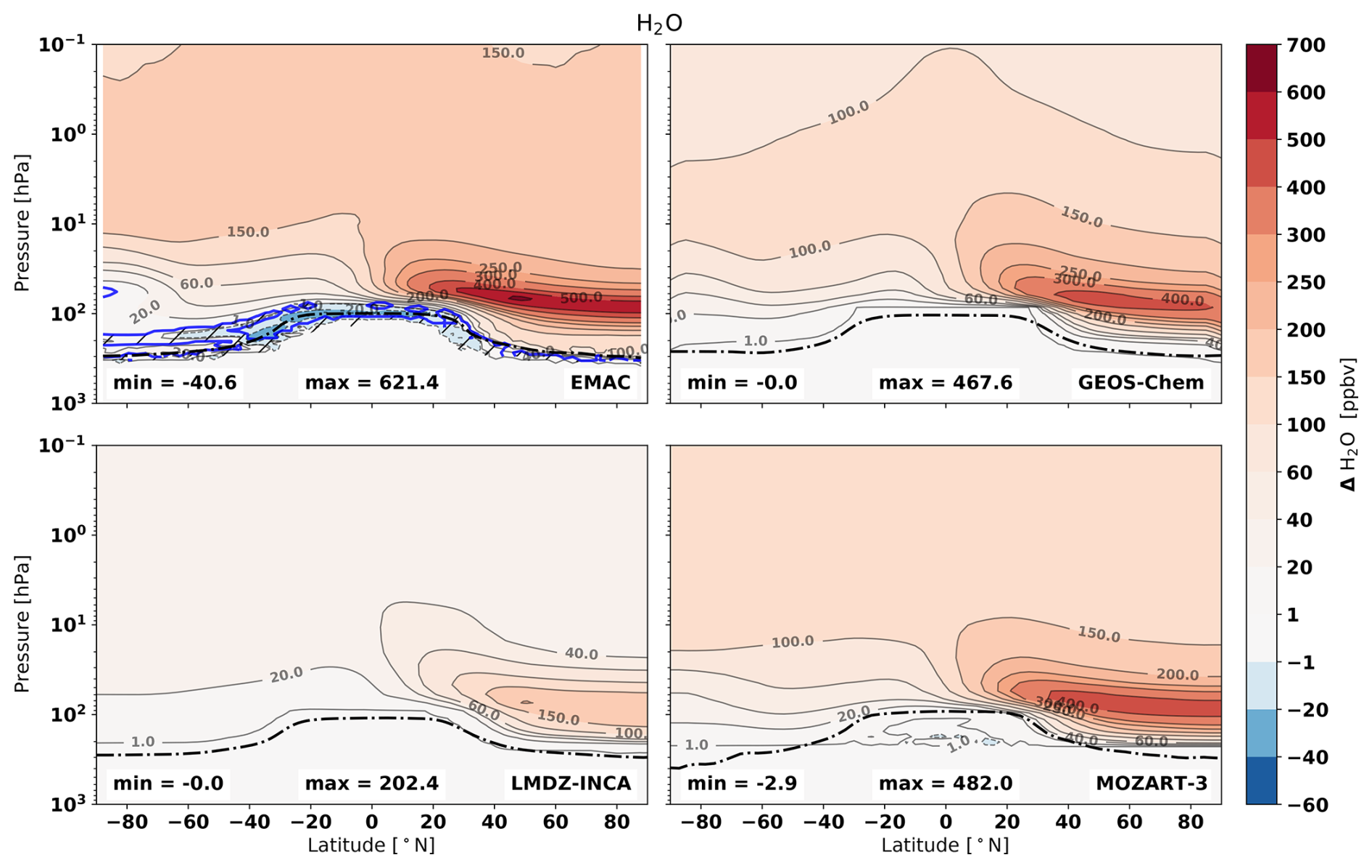
Figure 2 Zonal mean changes in water vapor mixing ratios (parts per billion by volume, ppbv) in response to the nominal supersonic emission scenario (S1). Hatched areas enclosed by blue lines indicate regions that are not statistically significant for the EMAC results. The dashed–dotted line indicates the mean tropopause pressure of each model. Similar figures for the triple-NO_x and low-cruise scenarios are provided in the Appendix (Figs. A3 and A4).

Between the models, we find a spread in the calculated water vapor perturbation lifetimes and hemispheric ratios that is indicative of the differences in the transport processes or chemical sinks between the models. Earlier works have identified that the model resolution is important to the representation of transport, mixing, and diffusion processes (Revell et al., 2015; Roeckner et al., 2006; Strahan and Polansky, 2006), and we also note a trend between the model grids and water vapor perturbation lifetimes and hemispheric ratios (Fig. 3). We find that the water vapor perturbation lifetime is linked to the model layer count between 400 and 50 hPa, with higher layer counts being associated with longer perturbation lifetimes. Transport of stratospheric water vapor emissions to the tropopause is a critical sink of the water vapor emissions, especially for the models using prescribed tropospheric water vapor mixing ratios (GEOS-Chem, LMDz–INCA, and MOZART-3), where the stratospheric water vapor tracer is effectively destroyed when it is transported into the model troposphere. We hypothesize that the vertical model grid affects the modeling of the stratospheric to tropospheric transport and, furthermore, that it introduces a secondary sink that affects stratospheric water vapor. During the model integration, the tropopause altitude evolves over time, which causes parts of the model grid to switch from the stratosphere (evolving tracers) to troposphere (prescribed ratios), stripping stratospheric tracers in the process. This has been noted to reduce the water vapor perturbation lifetimes of emissions near the tropopause in GEOS-Chem before (van 't Hoff et al., 2024), and it also explains why we find larger reductions (relative to the nominal scenario) in the water vapor perturbation lifetimes in the low-cruise scenario (S3) for the models with coarser vertical grids.

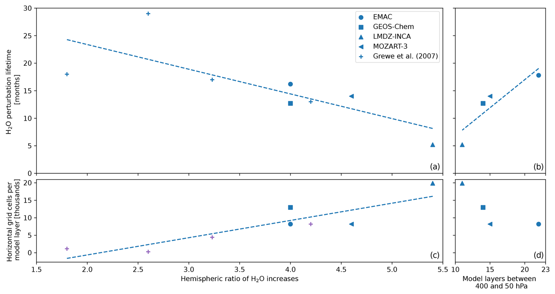
Figure 3 Comparison of the H₂O perturbation lifetime in months and the hemispheric ratio of the H₂O increases in the nominal supersonic scenario (S1) with vertical and horizontal model grid characteristics. Panel (a) shows the relationship between the perturbation lifetime and the hemispheric ratio, panel (b) shows the perturbation lifetime and the number of grid layers between 400 and 50 hPa, and panel (c) shows the hemispheric ratio and the horizontal grid fidelity. Panel (d) shows the vertical layer count against the horizontal grid fidelity. Markers denote the different models. Results from Grewe et al. (2007) are included for their equivalent scenario (S5; Grewe et al., 2007). The other emission scenarios are included in Fig. A5.

Figure 3 also shows that we find a trend between the hemispheric ratio and the horizontal grid fidelity. Strahan and Polansky (2006) found that the use of coarse horizontal grids led to overestimations of interhemispheric mixing in modeled atmospheres, and likewise, we find smaller hemispheric ratios in the coarser horizontal grids, suggesting that a larger share of the water vapor emissions are transported to the Southern Hemisphere. However, given the inverse relationship between the vertical and horizontal grid fidelities, we expect that this is primarily affected by the perturbation lifetime. The vast majority of water vapor emissions are in the Northern Hemisphere; therefore, shorter-perturbation lifetimes also reduce the transport of the water vapor perturbation to the Southern Hemisphere, increasing the hemispheric ratio. We also see these trends in the responses to the other emission scenarios (Fig. A5), indicating that differences in model grids may be a significant contributor to differences in the lifetime and transport of high-altitude water vapor emissions.

4.3 Nitrogen oxides and reactive nitrogen

Figure 4 shows the perturbation of nitrogen oxides (NO_x) and reactive nitrogen (${\mathrm{NO}}_{\mathrm{y}}=\mathrm{NO}+{\mathrm{NO}}_{\mathrm{2}}+{\mathrm{NO}}_{\mathrm{3}}+{\mathrm{HNO}}_{\mathrm{2}}+{\mathrm{HNO}}_{\mathrm{3}}+{\mathrm{HNO}}_{\mathrm{4}}+{\mathrm{ClNO}}_{\mathrm{3}}+\mathrm{2}{\mathrm{N}}_{\mathrm{2}}{\mathrm{O}}_{\mathrm{5}}+\mathrm{PAN}+{\mathrm{ClNO}}_{\mathrm{2}}+{\mathrm{BrNO}}_{\mathrm{3}}$) from the nominal supersonic scenario (S1) over the four models. Corresponding figures for the triple-NO_x and low-cruise scenarios are provided in the Appendix (Figs. A6 and A7). We find similar perturbations across all offline models. The NO_x responses are primarily concentrated around the Equator, with the strongest accumulation in the middle stratosphere and a secondary zone near the northern equatorial tropopause. In contrast to the NO_x perturbation, the accumulation of NO_y is concentrated around the region of cruise emissions. The NO_y perturbation, which includes that of NO_x, is mostly driven by increased formation of nitric acid (HNO₃) in these areas. NO_y is then transported to the North Pole or southwards to the tropical pipes (a region of upwelling over the tropics), where it makes its way to the middle stratosphere. This results in similar accumulation patterns for NO_y to what we find for the water vapor emissions.

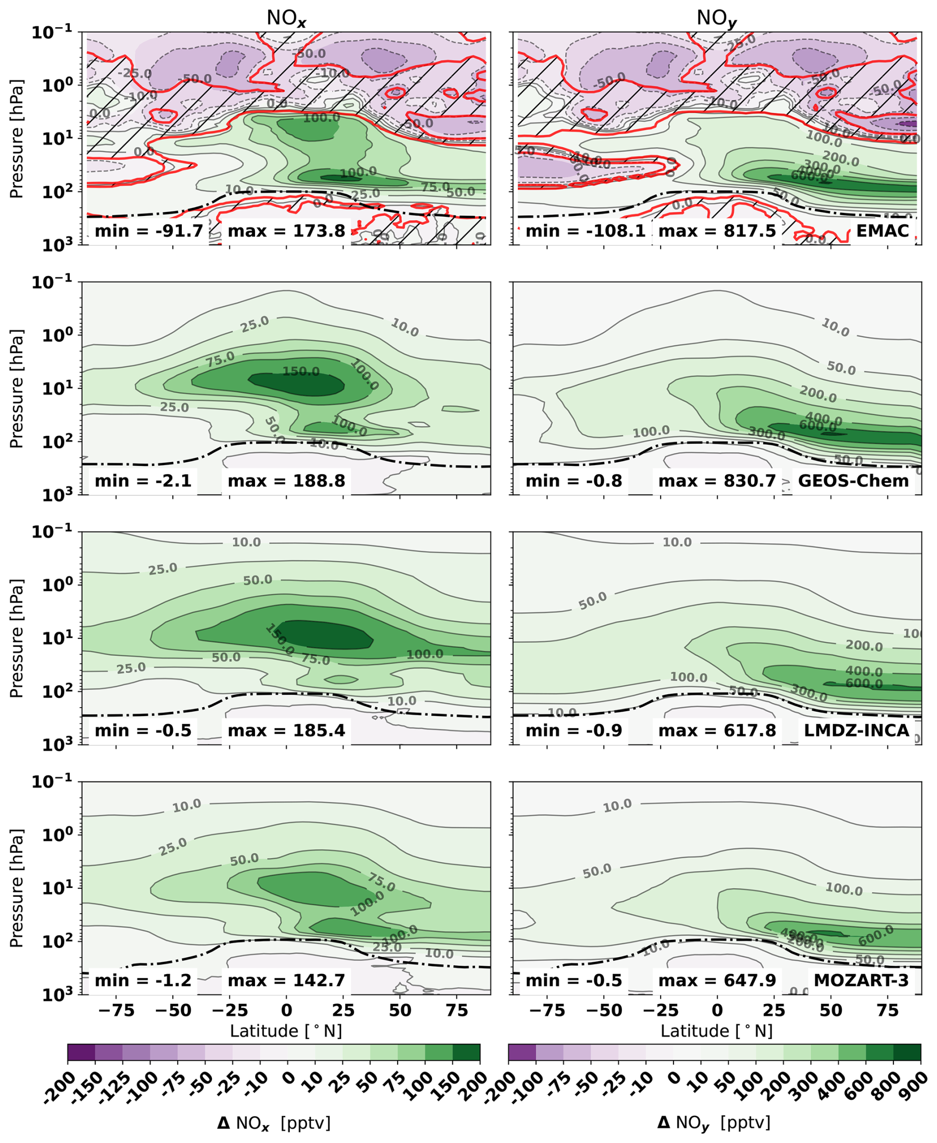
Figure 4 Zonal mean changes in NO_x (left) and NO_y (right) mixing ratios (parts per trillion by volume, pptv) in response to the nominal supersonic emissions (S1). Top to bottom: EMAC, GEOS-Chem, LMDz–INCA, and MOZART-3. Hatched areas enclosed by red lines indicate regions that are not statistically significant for the EMAC results. The dashed–dotted line indicates the mean tropopause pressure for each of the models. Figures for triple NO_x (S2) and low cruise (S3) scenarios are provided in the Appendix (Figs. A6, A7).

Contrary to the offline models, EMAC predicts that the SST adoption leads to the loss of NO_x and NO_y in the upper stratosphere and Southern Hemisphere for all supersonic scenarios (Figs. 4, A6, A7). We expect that these differences are predominantly driven by EMAC's use of online meteorology, which causes the deviation by meteorological parameters between the baseline and the perturbed model run due to a combined result of the butterfly effect (noise) and meteorological feedbacks from the changes in stratospheric composition (Deckert et al., 2011). Figure 5 shows the differences in the EMAC temperature fields. It shows that EMAC's stratosphere cools in response to the three supersonic scenarios. The stratospheric cooling has several effects on EMAC's chemistry, some of which are reflected in the NO_x response. Near the South Pole, we see indications that the cooling facilitates increased formation of PSCs. We find the regional depletion of gas-phase NO_y reservoirs associated with PSC chemistry (ClONO₂, HNO₃, and HNO₄) and increases in liquid-phase HNO₃ particles and solid-phase particles like nitric acid trihydrate (NAT). These changes suggest that PSC chemistry is enhanced, increasing the sedimentation of stratospheric nitrogen compounds and leading to denitrification of the southern stratosphere. This likely drives the loss of NO_x and NO_y over the South Pole. Near the North Pole, similar responses may occur, but this is hard to discern due to the proximity of the emission sources. Above pressure altitudes of 10 hPa, where nudging is no longer applied, there is stratospheric cooling of over −0.3 K in response to the nominal SST emissions. The cooling may contribute to the loss of NO_x and NO_y as it slows down the N-to-NO_x reformation reactions (Rosenfield and Douglass, 1998), but it likely also has more complex effects on the nitrogen chemistry cycles. Besides the change in temperature, there are also changes in EMAC's horizontal and vertical wind fields, but since these are nudged, they are predominantly statistically insignificant (Figs. A8 to A10). Some changes in wind fields can be seen above 10 hPa that may alter mixing in this region. Altogether, the use of online meteorology leads to a very different response of stratospheric NO_x and NO_y compared to the offline models. Given the sensitivity of ozone to NO_x, this is also linked to differences in the ozone response, which we discuss next.

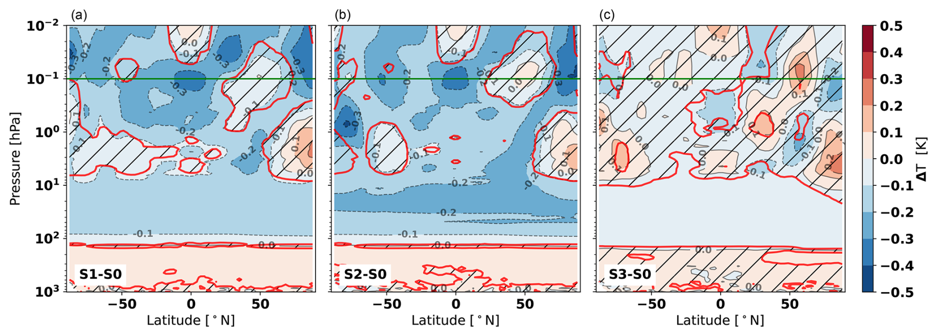
Figure 5 Zonal mean changes in temperature (in K) in the EMAC model, in response to the nominal (a), triple-NO_x (b), and low-cruise (S3) scenarios. Hatched areas enclosed by red lines indicate regions that are not statistically significant. The horizontal green line at 0.1 hPa indicates the upper pressure shown in other figures.

4.4 Ozone

Across all models and scenarios, we find increases in lower-stratospheric ozone mixing ratios paired with ozone depletion in the upper stratosphere (Fig. 6). Similar patterns are found for the other supersonic scenarios (Figs. 7, A11, A12). This pattern has been reported in several other studies, where the ozone increases in the lower stratosphere are attributed to NO_x-driven ozone formation and the ozone layer's self-healing effect (Zhang et al., 2023; Eastham et al., 2022; Fritz et al., 2022; Zhang et al., 2021b). This increase is strongest in the LMDz–INCA model, where the ozone increase spans both hemispheres. In GEOS-Chem and MOZART-3, this increase is limited to the equatorial lower stratosphere underneath the main lobe of ozone depletion, and in EMAC it only occurs in the Northern Hemisphere.

Figure 6 Mean changes in the ozone volume mixing ratio (ppbv) in response to the nominal supersonic (S1) emissions. Hatched areas enclosed by red lines indicate regions that are not statistically significant for the EMAC results. The dashed–dotted line indicates the mean tropopause pressure for each of the models. Similar figures for the triple-NO_x and low-cruise scenarios are provided in the Appendix (Figs. A11 and A12).

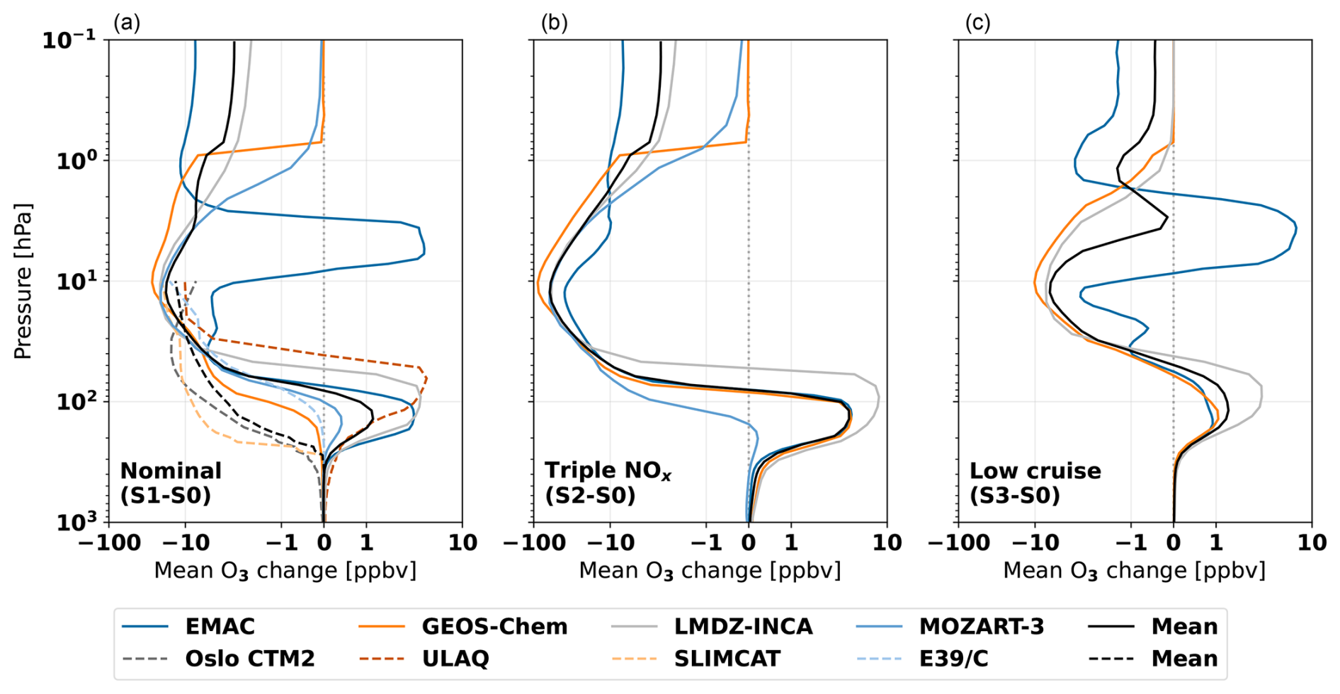
Figure 7 Mean changes in the ozone volume mixing ratio (ppbv) over altitude for the nominal supersonic (S1; (a)), triple-NO_x (S2; (b)), and low-cruise (S3; (c)) emission scenarios. Dashed lines show results from models used by Grewe et al. (2007).

When the supersonic NO_x emissions are tripled, the effect on ozone is enhanced, particularly over the tropics in the middle stratosphere (Fig. A11). We find that there is a nonlinear relationship between the SST NO_x emissions and the global ozone losses across all models. In GEOS-Chem and LMDz–INCA, the tripling of NO_x emissions increases stratospheric ozone budget losses (Table A3) by factors of 2.4 and 2.6, respectively, whereas these factors are 3.8 and 7.4 for MOZART-3 and EMAC. Between the offline models, MOZART-3 is most sensitive to NO_x emissions, which could be related to its lower background NO_x levels. In the low-cruise emission scenario, the magnitude of ozone increases, and losses are reduced (Fig. A12).

Similar to the NO_x and NO_y responses, EMAC's ozone response differs from the offline models (Figs. 6, 7), which is likely coupled to feedbacks with its online meteorology. The most notable difference is the presence of ozone increases at high northern and southern latitudes above 10 hPa, with both being partially statistically significant. We hypothesize that their formation is driven by the previously discussed stratospheric cooling and enhancements of PSC chemistry. In the Southern Hemisphere, the meteorological feedbacks cause shifts in the abundance of nitrogen and chlorine (ClONO₂) reservoir species that correlate with areas of ozone changes. In the northern lower stratosphere, the ozone increase correlates with an increase in the HNO₃ formation. The patterns that should be associated with PSC chemistry tend to vanish for the triple-NO_x emission scenario (Fig. A11), which may point towards their limited magnitude. The regions of ozone increases could also be related to slowdowns of the Chapman mechanism due to cooling and perturbations of local transport (Kirner et al., 2014). The former is also seen in the odd O_x loss rates, which are evaluated in the next section.

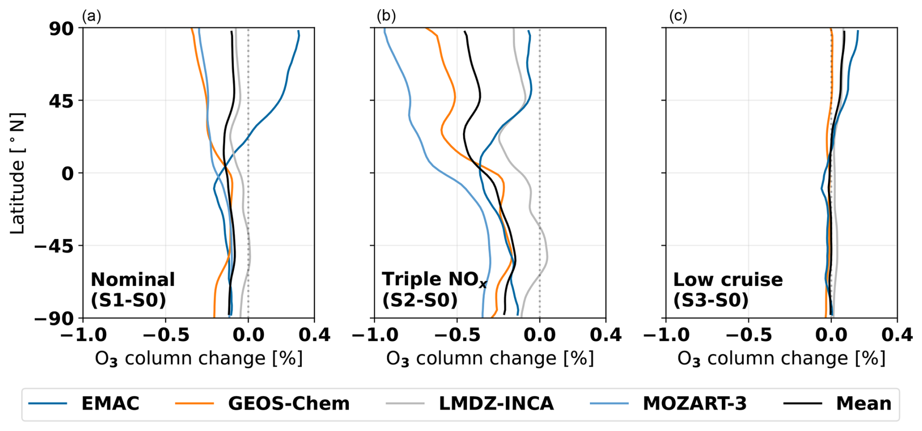
Figure 8 Zonal mean annually averaged changes in the ozone columns (percentage) for nominal supersonic (S1; (a)), triple-NO_x (S2; (b)), and low-cruise (S3; (c)) emission scenarios.

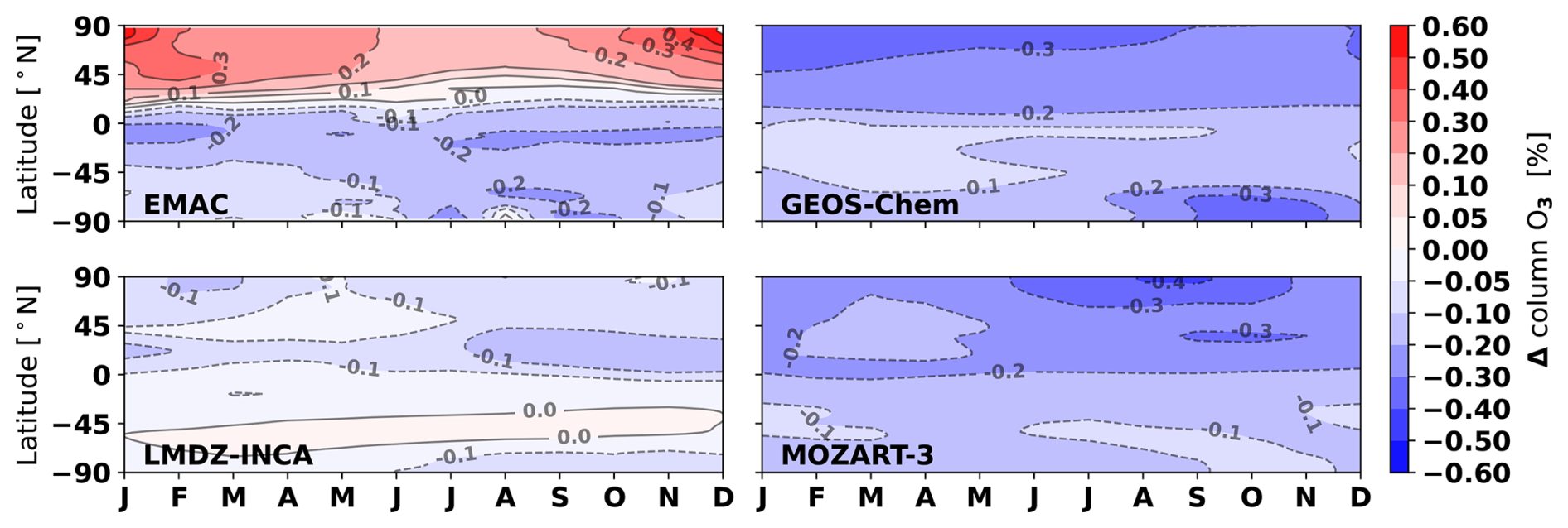
Figure 9 Mean monthly changes in the ozone columns (percentage) in response to the nominal supersonic emission scenario (S1–S0). Similar figures for the other emission scenarios are provided in the Appendix (Figs. A13 and A14).

Differences between the model responses become more evident when the changes in the ozone columns are compared. Figure 8 shows the mean ozone column change over latitude for the emission scenarios alongside the multi-model mean profile. It shows that the spread between the models is largest in the Northern Hemisphere for all emission scenarios, particularly near the North Pole. After expanding this into seasonal ozone column changes (Fig. 9), we find that all models show different seasonal behavior as well. For example, GEOS-Chem shows an enhancement of ozone column loss during the Arctic and Antarctic ozone hole formation. These enhancements are also present in LMDz–INCA, albeit at a smaller scale. MOZART-3 does not show them, and it instead calculates the highest Arctic ozone depletion from June to November. EMAC shows year-round increases in the ozone column in the Northern Hemisphere. We expect that such differences are the results of differences in the modeling of processes important to ozone, such as the PSC processes and feedbacks from emissions on heterogeneous chemistry. Only GEOS-Chem and LMDz–INCA capture the effect of the emissions on the available surface area for heterogeneous chemistry, which may explain why only these models show enhancement of seasonal ozone holes. The differences may further be affected by the availability of stratospheric halogens (Table A4). For example, the enhancement of the ozone hole is stronger in GEOS-Chem, which also has higher stratospheric halogen availability.

4.5 Odd oxygen loss

To better understand the source of the differences in the ozone responses, we evaluate the changes in odd oxygen (O_x) reaction rates for EMAC, GEOS-Chem, and LMDz–INCA. For this, we use the same reaction grouping as Zhang et al. (2023, 2021a). All our models show that the supersonic scenarios lead to net increases in the O_x loss. When averaged over altitude, we find similar baseline O_x loss rates across all models (Fig. 10), and the responses of the GEOS-Chem and LMDz–INCA models appear to share similar profiles, whereas that of EMAC is very different. When the O_x loss responses are seen as zonal averages (Fig. 11), further differences in the spatial distribution of the O_x loss responses become evident.

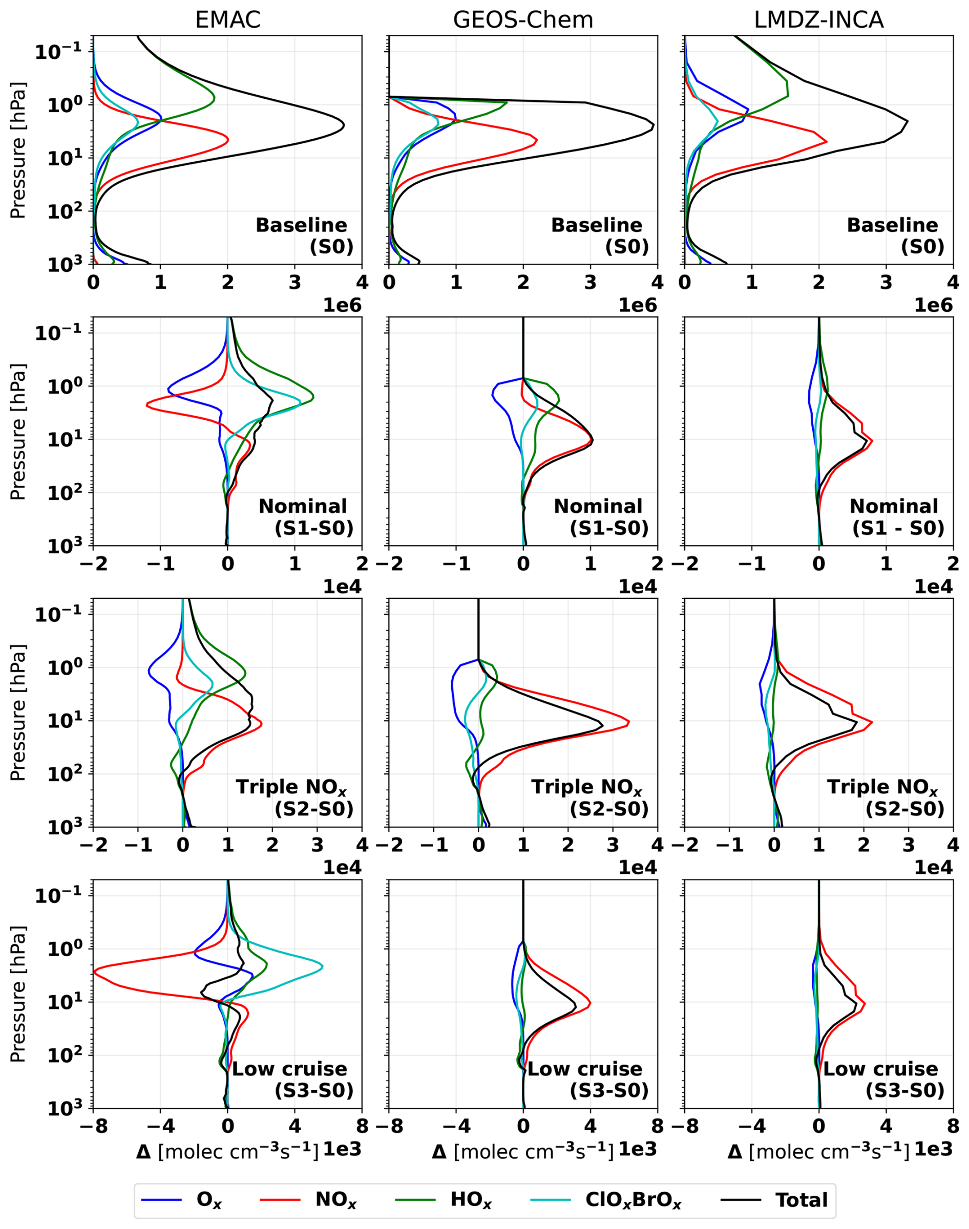
Figure 10 Mean background O_x loss rates (top) and O_x loss rate perturbations from emission scenarios over the pressure altitude for EMAC (left), GEOS-Chem (middle), and LMDz–INCA (right). From top to bottom: background loss rates, loss rate perturbation from nominal supersonic emissions (S1), loss rate perturbation from triple-NO_x emissions (S2), and loss rate perturbation from low-cruise emissions (S3).

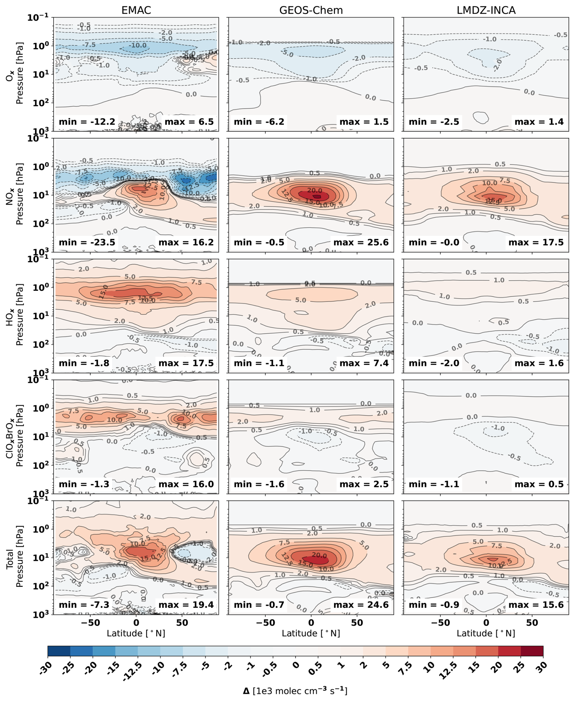
Figure 11 Zonal average mean changes in O_x loss reactions in response to the nominal supersonic emissions for EMAC (left), GEOS-Chem (middle), and LMDz–INCA (right). Loss perturbations are split into O_x-driven loss (top), NO_x-driven loss (second row), HO_x-driven loss (third), ClO_xBrO_x-driven loss (fourth), and total changes in O_x loss (bottom). Values are given in thousands of molec. cm⁻³ s⁻¹. Similar figures for the triple-NO_x (S2) and low-cruise (S3) scenarios are provided in the Appendix (Figs. A15 and A16).

The O_x loss reaction responses of the GEOS-Chem and LMDz–INCA models are similar. In these models, the largest response to the nominal scenario is an increase in NO_x-driven O_x losses from 200 to 20 hPa. HO_x-driven losses also increase but mostly at higher altitudes from 20 to 0.1 hPa. These increases are paired with decreases in O_x–O_x losses as the availability of O_x reduces. The models also calculate increases in ClO_x- and BrO_x-driven losses above 10 hPa. In response to the triple-NO_x scenario, the NO_x-driven O_x losses increase by around 3-fold, reducing the effect on ClO_x- and BrO_x-driven losses. For the lower-cruise-altitude scenario (S3), we find similar changes in O_x loss rates to the nominal supersonic scenario but at smaller magnitudes. In the case of the GEOS-Chem and LMDz–INCA models, the reduction in cruise altitude also sharply reduces HO_x-driven O_x losses. This is related to the shorter water vapor perturbation lifetimes at this cruise altitude.

Figures 10 and 11 show that the increased complexity of EMAC's response extends to odd O_x loss rates. Contrary to the previously shown changes in the ozone and NO_x mixing ratios, the response in EMAC's O_x loss reactions is entirely statistically significant. Both figures show that there are areas where NO_x-driven O_x losses are reduced, coinciding with the previously discussed areas of denitrification in the upper stratosphere and over the South Pole (Fig. 4). The reduction in NO_x-driven O_x losses is coupled with local increases in HO_x and ClO_x- and BrO_x-driven losses, the latter of which is also affected by the enhancement of PSC chemistry. The cooling of the stratosphere also slows the Chapman mechanism, leading to reductions in upper-stratospheric O_x–O_x losses, with the exceptions of the areas in which there is a net increase in ozone and therefore also O_x availability.

The perturbation of ClO_xBrO_x-driven O_x losses differs across the three models, with EMAC's ClO_xBrO_x response showing peak values up to 5 times larger than GEOS-Chem, whereas ClO_xBrO_x losses are mostly unaffected in LMDz–INCA. The large response in EMAC is likely coupled to the local decreases in NO_x-driven losses in these areas that are of a similar magnitude (Fig. 11). Between GEOS-Chem and LMDz–INCA, we expect that these differences may be related to the availability and distribution of halogens. Table A4 (Appendix) shows the mean background mixing ratios for key halogens at the surface and from 200 to 10 hPa in the models' baseline atmospheres. While we find similar background halogen levels near the surface, GEOS-Chem has lower stratospheric chlorofluorocarbon (CFC) mixing ratios and higher values of other halogens compared to LMDz–INCA. This could suggest that the CFC destruction is faster GEOS-Chem, which may affect the role of ClO_xBrO_x-driven O_x losses. Another difference is the upper limit of the O_x chemistry domain, which is around 1 hPa in GEOS-Chem but extends further in the other models. Above this altitude, GEOS-Chem has no O_x chemistry, yet other species related to ozone chemistry are allowed to evolve freely. This may lead to an accumulation of HO_x and halogens in the mesosphere, contributing to increased HO_x and ClO_xBrO_x-driven O_x losses when they are transported downwards into the region of O_x chemistry.

4.6 Radiative forcing

From non-CO₂ emissions, we estimate a net warming effect of 13.9 mW m⁻² for the nominal supersonic scenario (S1). This is predominantly driven by the accumulation of stratospheric water vapor (20.8 mW m⁻²) and warming from changes in the distribution of ozone (3.2 mW m⁻²). The calculated ozone forcing ranges from 1.3 mW m⁻² (GEOS-Chem) to 6.8 mW m⁻² (LMDz–INCA), where EMAC and MOZART-3 find forcings of 3.0 and 2.2 mW m⁻², respectively. The largest spread is in the water vapor forcing, ranging from 6.2 mW m⁻² (LMDz–INCA) to 32.4 mW m⁻² (MOZART-3). This is affected not only by the differences in water vapor perturbation lifetime within the models, but also by the radiative schemes used to assess RF. For example, the two radiative schemes applied to EMAC find water vapor forcings of 29.7 and 22.2 mW m⁻² in this scenario, which is a relative difference of 33 %. The SOCRATES model used with MOZART-3 also finds a larger water vapor forcing relative to the water vapor perturbation and lifetime. This suggests that the differences between radiative schemes may be a more important contributor to uncertainties in radiative forcing assessments than differences in atmospheric perturbations calculated by CTMs or CCMs.

Only the GEOS-Chem and LMDz–INCA models assess the effect of aerosols on RF, and the aerosol perturbations in these models are shown in Figs. A17 and A18. These models do assess aerosol RF at different altitudes, which causes them to find different forcing from BC aerosols (Eastham et al., 2022; Speth et al., 2021). For the nominal scenario, LMDz–INCA calculates RF of 0.5 mW m⁻² from BC and −10.0 mW m⁻² from inorganic aerosols, and GEOS-Chem calculates −1.3 and −9.3 mW m⁻², respectively. Between the models, we calculate a mean aerosol forcing of −10.1 mW m⁻², resulting in a net forcing of 13.9 mW m⁻² from the nominal supersonic scenario. Considering the altitude dependency of the BC forcing, this value may change by up to ±0.5 mW m⁻², depending on the assessment altitude.

The tripling of NO_x emissions (S2) affects the radiative effect of ozone, which increases to a model mean of 11.4 mW m⁻² (range from 6.9 to 20.9). In this case, we calculate model mean RF from water vapor of 18.2 mW m⁻² (model range from 6.3 to 31.1) and RF from aerosols of −0.4 mW m⁻² for BC and −9.7 mW m⁻² for inorganic aerosols. This results in a model mean net RF of 19.4 mW m⁻² from non-CO₂ emissions (model range from 16.7 to 28.1). The reduction in the cruise altitude and speed (S3) reduces the RF from ozone to 2.9 mW m⁻² (model range from 2.1 to 4.6) and water vapor to 4.3 mW m⁻² (model range from 0.7 to 8.2). RF from aerosols is also smaller, with −0.1 mW m⁻² from BC and −3.3 mW m⁻² from inorganic aerosols. This results in a model mean net RF of 3.8 mW m⁻² from non-CO₂ emissions (range from 0.5 to 7.1).

5 Discussion

Across all models and assessments, we find that the partial replacement of subsonic aviation with supersonic aircraft leads to extensive changes to the atmospheric composition, particularly in the stratosphere, and global radiation forcing. The magnitude of these changes scales with fleet-wide NO_x emissions and the cruise altitude across all models. Therefore, we also find the largest effect on the ozone column and RF in response to the Mach 2 concept with higher NO_x emissions (Scenario S2). In terms of NO_x emissions, this scenario is closest to the SST concepts studied in other recent works (Zhang et al., 2023, 2021a; Eastham et al., 2022; Speth et al., 2021), which is why we consider it a basis for comparison with the literature and the most plausible outlook for future SST adoption.

The stratospheric changes we identify in response to the S2 scenario match patterns identified in several recent works (van 't Hoff et al., 2024; Zhang et al., 2023, 2021a; Eastham et al., 2022; Kinnison et al., 2020). Here, we find a model mean change in the global ozone column of −0.3 % (−0.9 DU). Scaling by fuel consumption, this is similar to the −0.74 % ozone column loss reported by Zhang et al. (2023), who considered a larger SST fleet with around 2.1 times the fuel burn. It does not match with results from Eastham et al. (2022), who reported a larger ozone column loss (−0.77 %) for a smaller SST fleet (14.9 Tg of annual SST fuel burn). This may be related to differences in background conditions and in the emission scenarios. The scenarios considered by Eastham et al. (2022) have higher SST NO_x emissions, and they consider a more prominent role of the Asian market in SST adoption than the inventories we use, displacing more SST traffic to lower latitudes (Speth et al., 2021). The ozone column is substantially more sensitive to SST emissions near the tropics (van 't Hoff et al., 2024; Fritz et al., 2022), which may explain why they find higher ozone loss relative to the fuel consumption. The nominal and triple-NO_x scenarios we evaluate are also similar to scenarios evaluated by Zhang et al. (2021b; cases A and C). In comparison to their results, we find also find similar ozone column losses (−0.1 % and −0.3 %, compared to their −0.2 % and −0.4 %). We also find similar O_x loss rate perturbations, in particular between GEOS-Chem and the WACCM4 model they used. Several recent studies have identified that the perturbation of ozone can be the primary source of radiative forcing from SST emissions (van 't Hoff et al., 2024; Zhang et al., 2023; Eastham et al., 2022), but we instead find water vapor to be dominant in all scenarios, matching the results from Zhang et al. (2021b) and Grewe et al. (2007). This is not agreed upon in all models, however, as in some cases LMDz–INCA and GEOS-Chem find that the ozone perturbation is the primary forcer (scenarios S1 to S3 for LMDz–INCA and scenario S3 for GEOS-Chem). We expect that this difference is related to fleet-wide NO_x emissions. Previous works have shown that RF from ozone perturbations scales with fleet-wide NO_x emissions (van 't Hoff et al., 2024; Zhang et al., 2021b), and even in the triple-NO_x scenario, our NO_x emissions index is lower than indices used by the works that find forcing from ozone to be dominant (van 't Hoff et al., 2024; Zhang et al., 2023; Eastham et al., 2022). Therefore, it is plausible that we'd also find the primary radiative effect to be from ozone if higher supersonic NO_x emissions are considered.

Since the nominal scenario that we consider is almost identical to scenario S5 from Grewe et al. (2007), we also compare our results to their results, although we note that there are considerable differences between our models and the ones they used. For example, our models have higher resolutions (horizontal and vertical) and upper-grid levels (0.1 to 0.01 hPa compared to their 10 hPa). Compared to their results, we find lower-stratospheric perturbations of water vapor (47 Tg compared to 64 Tg) and ozone (−3.1 Tg compared to −8 Tg). Considering the perturbation mass and the hemispheric ratios, we also find a smaller spread in our models compared to theirs (Fig. A19). In terms of radiative forcing, we calculate this at the tropopause level, whereas they calculated it at the top of the atmosphere, hindering direct comparison. For the scattering inorganic aerosols, which should not be affected much by the assessment altitude, we find similar RF (−9.7 mW m⁻² compared to their −11.4 mW m⁻²). At the top of the atmosphere, we find smaller RF for black carbon (0.5 mW m⁻² for LMDz–INCA and 1.7 mW m⁻² for GEOS-Chem compared to their 4.8 mW m⁻²), which could be related to differences in radiative modeling, aerosol size distributions, or the simulated transport of the black carbon.

Like earlier works, we find that the perturbation of stratospheric water vapor plays a key role in the radiative effect of SSTs (Zhang et al., 2023; Eastham et al., 2022; Matthes et al., 2022; Grewe et al., 2007), but we note that RF from water vapor is prone to several uncertainties. Foremost, we find that the RF depends on the radiative schemes, with relative differences of up to 30 % between the two radiative schemes that we apply to the EMAC model atmospheres. The radiative effect from water vapor is also directly related to the stratospheric water vapor burden, and therefore, it depends on the water vapor perturbation lifetime within the models. We find indications that this lifetime is affected by the vertical resolution and model grid, linking higher numbers of grid layers between 400 and 50 hPa to higher perturbation lifetimes. Therefore, our results suggest that the model grid itself and the choice of radiative scheme may be important contributors to uncertainties surrounding radiative effects of water vapor emissions. We expect that these factors may be influential in all assessments of high-altitude water vapor emissions and not exclusive to supersonic aircraft.

We find considerable differences between the responses of the online and offline models. Between the offline models (GEOS-Chem, LMDz–INCA, and MOZART-3), we find good agreement in all perturbations of the stratospheric composition. The most notable difference is the lower vertical domain of GEOS-Chem's stratospheric ozone chemistry, which may lead to an increased influx of HO_x at the upper-stratospheric boundary, although our results do not indicate that this has a large effect on the calculated ozone column responses. Comparing the online EMAC model to the offline models, we see some substantial differences from the inclusion of meteorological feedbacks (predominantly stratospheric cooling) on chemistry. The inclusion of this feedback allows EMAC to capture interactions that are not included in the offline models. For example, we find that the stratospheric cooling enhances PSC chemistry in EMAC, leading to denitrification over the South Pole in response to the SST adoption. To our knowledge, this feedback from SST emissions has not previously been identified in earlier works. We also identify denitrification of the upper stratosphere in response to the SST emissions, likely due to slowdown of NO_x reformation reactions and interactions with nitrogen chemistry cycles. This contributes to increases in upper-stratospheric ozone at high latitudes, which has also been shown in other works that use EMAC in a similar configuration (Pletzer et al., 2022; Kirner et al., 2014). We find these differences even when the meteorological feedbacks are still constrained. Within the model, the horizontal and vertical winds are still nudged for the majority of the stratosphere, and furthermore, some feedbacks like local temperature changes from black carbon perturbations are not included. The inclusion of these feedbacks would likely further alter the response to high-altitude emissions. We expect that the consideration of meteorological feedbacks might be critical to the complete assessment of the effects of high-altitude emissions as some important feedbacks may be overlooked otherwise.

The adoption of a fleet of SSTs should be considered in the context of other options for air travel in terms of their CO₂ and non-CO₂ effects. For the SST emissions in the nominal and triple-NO_x scenarios, we calculate a fuel burn-to-RPK ratio of 79.3 g $/$ RPK and for the low-cruise SST a ratio of 58.0 g $/$ RPK. In comparison, for the subsonic aircraft (scenario S0), we calculate a ratio of 36.8 g $/$ RPK, which is in agreement with the ratio of 38.0 g $/$ RPK for subsonic aviation in 2018 that can be calculated from the results of Lee et al. (2021). This suggests that replacing a RPK with these SST concepts increases the associated fuel consumption, and by extension the emission of CO₂ and its radiative effects, by 109 % and 53 % for the respective nominal and low-cruise concepts. A similar trend also holds for the radiative effects of non-CO₂ emissions. In the triple-NO_x scenario, we find that replacing 7.3 × 10¹¹ subsonic RPK with SSTs increases the RF from non-CO₂ emissions by 19.4 mW m⁻². From this, we calculate an increase in the RF : RPK ratio of 26.6 × 10⁻¹² mW m⁻² $/$ RPK. In the case of the nominal and low-cruise scenarios, we find increases in this ratio of 19.0 × 10⁻¹² and 5.2 × 10⁻¹² mW m⁻² $/$ RPK, respectively. These estimates incorporate the removal of the equivalent RPKs from the subsonic fleet, thereby representing the additional RF from non-CO₂ emissions per RPK when an RPK is flown by a SST rather than a subsonic aircraft. We note that our results do not reflect the RF benefits of practically eliminating contrail impacts from the subsonic RPK but do reflect changes in aerosol RF. In comparison, using non-CO₂ RF estimates from the 2018 subsonic aviation from Lee et al. (2021), we calculate a RF : RPK ratio of 14.4 × 10⁻¹² mW m⁻² $/$ RPK for subsonic radiative effects from non-CO₂ emissions. Our results therefore indicate that the replacement of subsonic RPKs with the triple-NO_x scenario SST would increase the non-CO₂ RF : RPK ratio by 185 % compared to the estimate of Lee et al. (2021) and that the nominal SST and low-cruise (Mach 1.6) SST would increase the RPK cost by 132 % and 36 %, respectively. These discrepancies would differ if contrails were to be included in the RF assessment, but they provide an estimate of the additional climate impacts of SSTs over subsonic aircraft. The disparity that we identify has also been reported in earlier works (Eastham et al., 2022; Speth et al., 2021; Grewe et al., 2007), and while our results suggest that this disparity may be mitigated by reducing supersonic NO_x emissions, cruise speed, and altitude, we expect it will nonetheless persist due to the more sensitive emission altitudes, the higher fuel requirements, and the lower passenger numbers of supersonic aircraft.

Our results provide some actionable information for consideration in sustainability discussions related to SSTs. We find the atmospheric and radiative effects are predominantly driven by NO_x and water vapor emissions, indicating that the use of sustainable aviation fuels is not likely to lead to substantial differences in these effects. On the contrary, sustainable aviation fuels are likely to have lower sulfur and black carbon emissions, which will increase SST radiative effects by reducing the emissions responsible for the cooling RF, as also identified by Speth et al. (2021). We also remark that the effect on the ozone column could be considered in the context of the effects on human health. For example, in response to the triple-NO_x scenario, we find a model mean global ozone column loss of −0.3 % (−0.9 DU), but some models calculate the year-round depletion of up to −0.7 % (−2.1 DU) over the Northern Hemisphere. Considering the distribution of the population, the effect on human health is likely larger than what the global average would imply. Estimating the effect on human health lies outside of the scope of this work, but it may be an effective means to communicate the effect of changes in the ozone column. Such an approach may also account for the changes in air quality from tropospheric ozone perturbations that are otherwise not included in discussions surrounding global column ozone perturbations.

6 Conclusions

For the first time since 2007, we present a comprehensive multi-model assessment of the effects of the partial replacement of subsonic aviation traffic with a fleet of supersonic transport aircraft on atmospheric composition and global radiative forcing. With four widely used models (EMAC, LMDz–INCA, GEOS-Chem, and MOZART-3), we evaluate three supersonic adoption scenarios based on the emission scenarios of the SCENIC project (Grewe et al., 2007). Two of these scenarios consider the adoption of a Mach 2 supersonic aircraft operating at cruise altitudes from 16.5 to 19.5 km to replace around 4 % of subsonic aviation traffic, differing from fleet-wide NO_x emissions (13.80 and 4.60 g (NO₂) kg⁻¹). The third scenario considers aircraft with a lower cruise speed (Mach 1.6) and lower altitude instead (13.1 to 16.7 km).

The partial replacement of subsonic aviation with both Mach 2 concepts results in a reduction in the global ozone column. For the Mach 2 concept with NO_x emissions of 13.80 g (NO₂) kg⁻¹, we calculate the model mean global ozone column loss of −0.3 % (−0.9 DU), with higher losses across the Northern Hemisphere (model mean up to −0.5 %; −1.5 DU). The replacement of subsonic aviation with this concept increases radiative forcing by 19.4 mW m⁻². The biggest forcing is from changes in stratospheric water vapor (18.2 mW m⁻²), followed by ozone (11.4 mW m⁻²), and aerosols (−10.2 mW m⁻²). If the fleet-wide NO_x emissions are reduced by 67 %, the net forcing also reduces to 13.9 mW m⁻² because of the smaller ozone perturbation (−0.1 % (−0.3 DU)) and its associated forcing (3.2 mW m⁻²). If part of the subsonic aviation is instead replaced by the Mach 1.6 concept, which has a lower cruise altitude and fleet-wide NO_x emissions, the effects on stratospheric composition and radiative forcing are reduced by 3.8 mW m⁻². These values do not account for potential changes in contrail formation and the increase in CO₂ emissions. Compared to estimates of subsonic aviation, we find that the replacement of subsonic passenger revenue kilometers with supersonic aircraft increases the associated radiative forcing from non-CO₂ emissions by up to 185 %.

Compared to the previous multi-model assessment of the atmospheric and radiative effects of supersonic aircraft (Grewe et al., 2007), we see a narrower spread in our model evaluations of the water vapor and ozone perturbations. We find good agreement in the composition changes between the three models which use offline meteorology, but we also see large differences with the model with online meteorology (EMAC). The inclusion of meteorological feedbacks in the model captures several responses to the emissions that are not captured in the offline models, such as the denitrification of the upper stratosphere and South Pole. These feedbacks have substantial effects on the stratospheric ozone and nitrogen responses, and we expect that they may be of critical importance to the assessment of the effects of high-altitude emissions.

Appendix A

Table A1 Summary of stratospheric H₂O perturbations due to the emission scenarios. Values are calculated as triannual averages.

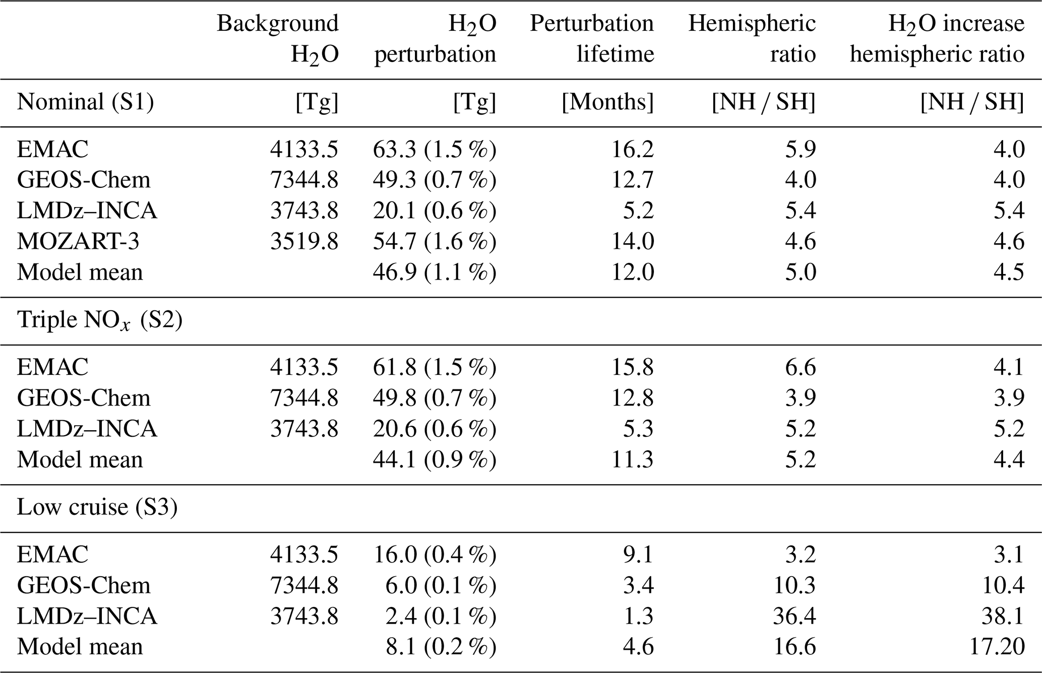
Table A2 Summary of stratospheric NO_x perturbations due to the emission scenarios. Values are calculated as triannual averages.

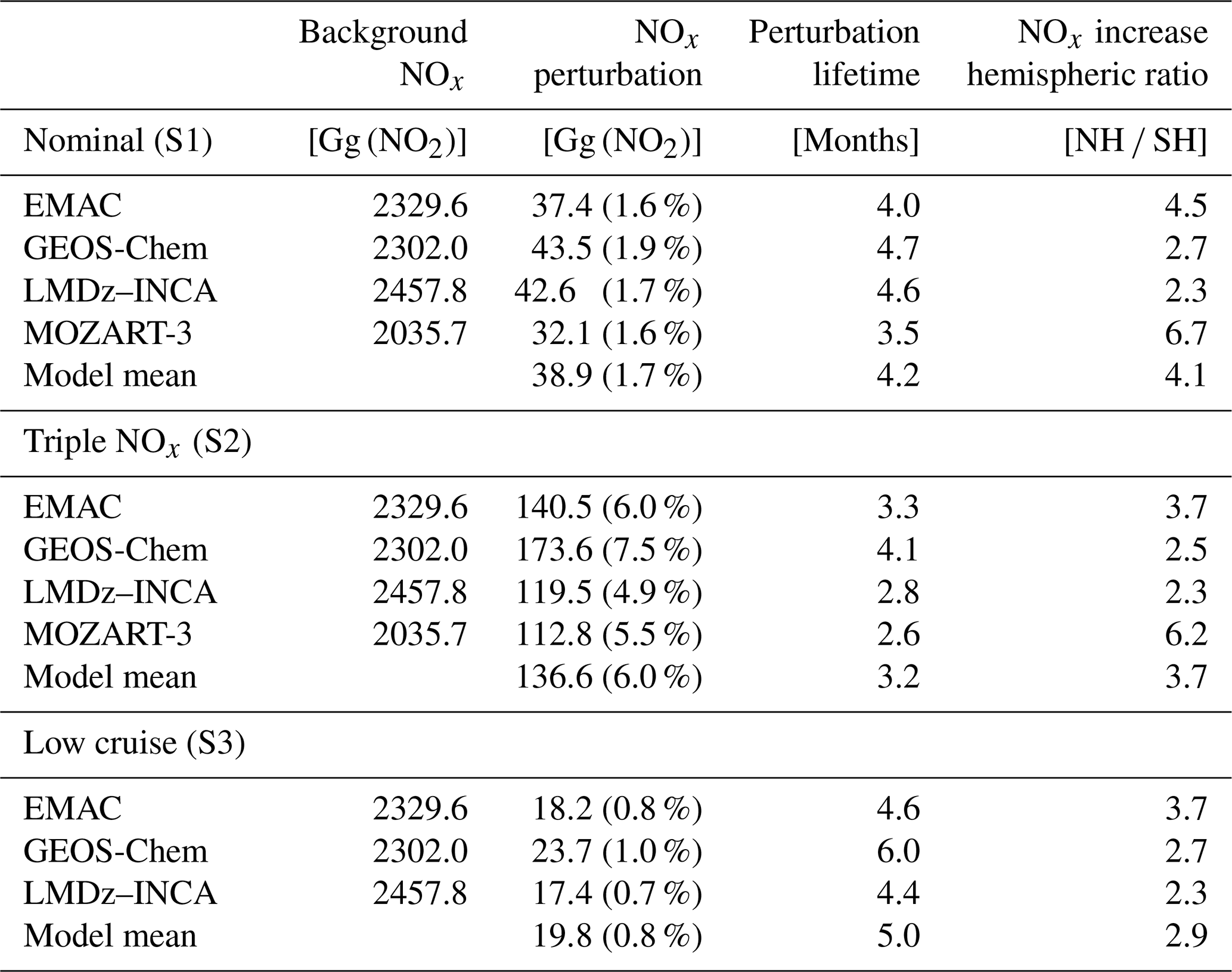
Table A3 Summary of O₃ perturbations due to the emission scenarios. Values are calculated as triannual averages.

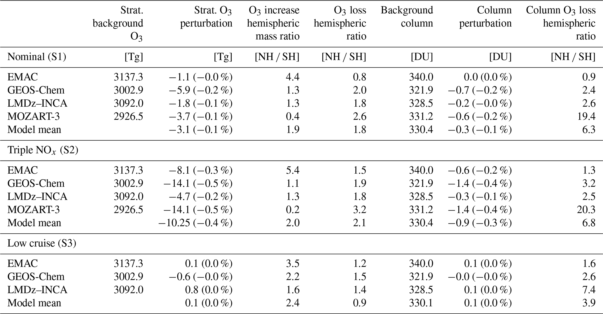
Table A4 Summary of mean background halogen mixing ratios in the last 3 years of the baseline (S0) scenario. Units in parts per trillion by volume (pptv). Values denoted by “–” indicate species which are not present in that model.

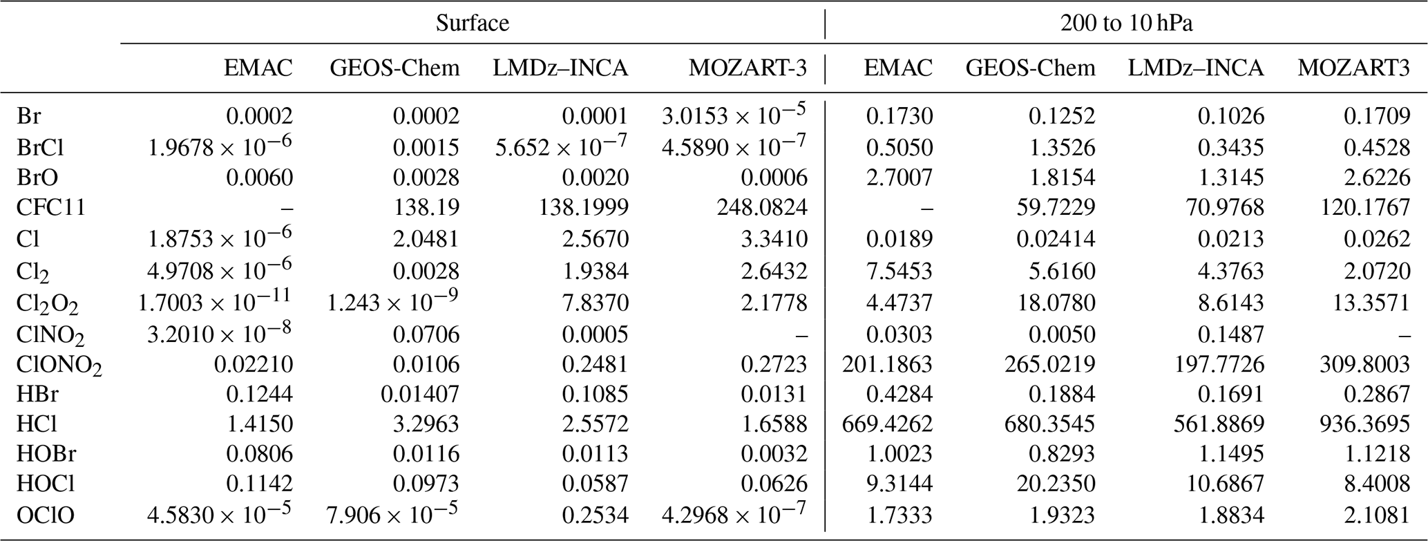
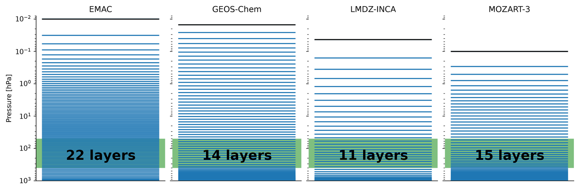
Figure A1 Comparison of the vertical grid of the EMAC, GEOS-Chem, LMDz–INCA, and MOZART-3 models. The green region denotes the region between 400 and 50 hPa, which is important to the stratospheric–tropospheric exchange. The count of model layers within this region is shown in the figure.

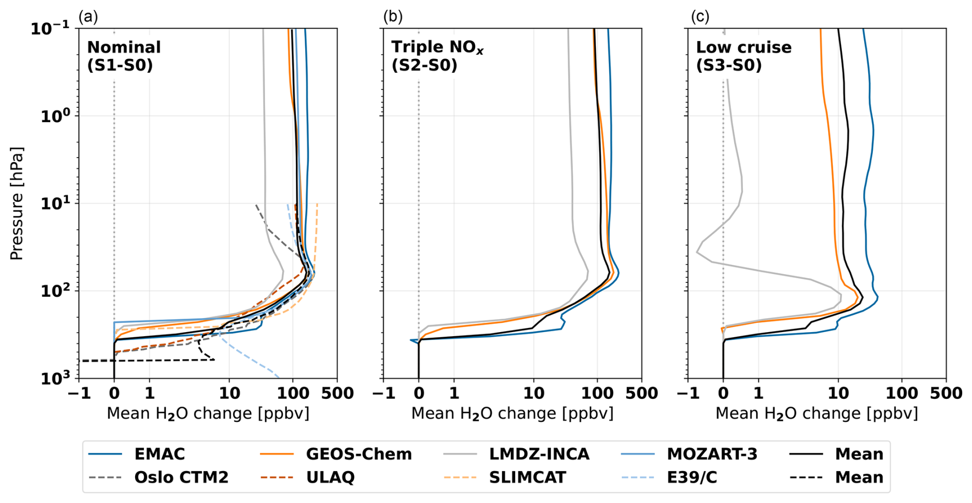
Figure A2 Mean changes in the water vapor mixing ratio over altitude for the nominal supersonic (S1; (a)), triple-NO_x (S2; (b)), and low-cruise (S3; (c)) emission scenarios. Entries with dashed lines are from data from Grewe et al. (2007).

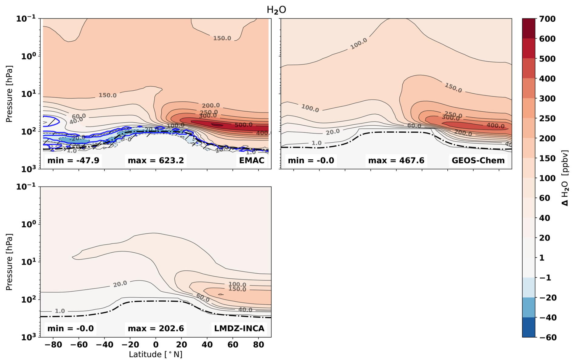
Figure A3 Changes in H₂O volume mixing ratios for the triple-NO_x (S2) emission scenario. Hatched areas enclosed by blue lines indicate regions that are not statistically significant for the EMAC results. Dashed–dotted lines show the mean tropopause pressure that is calculated per model.

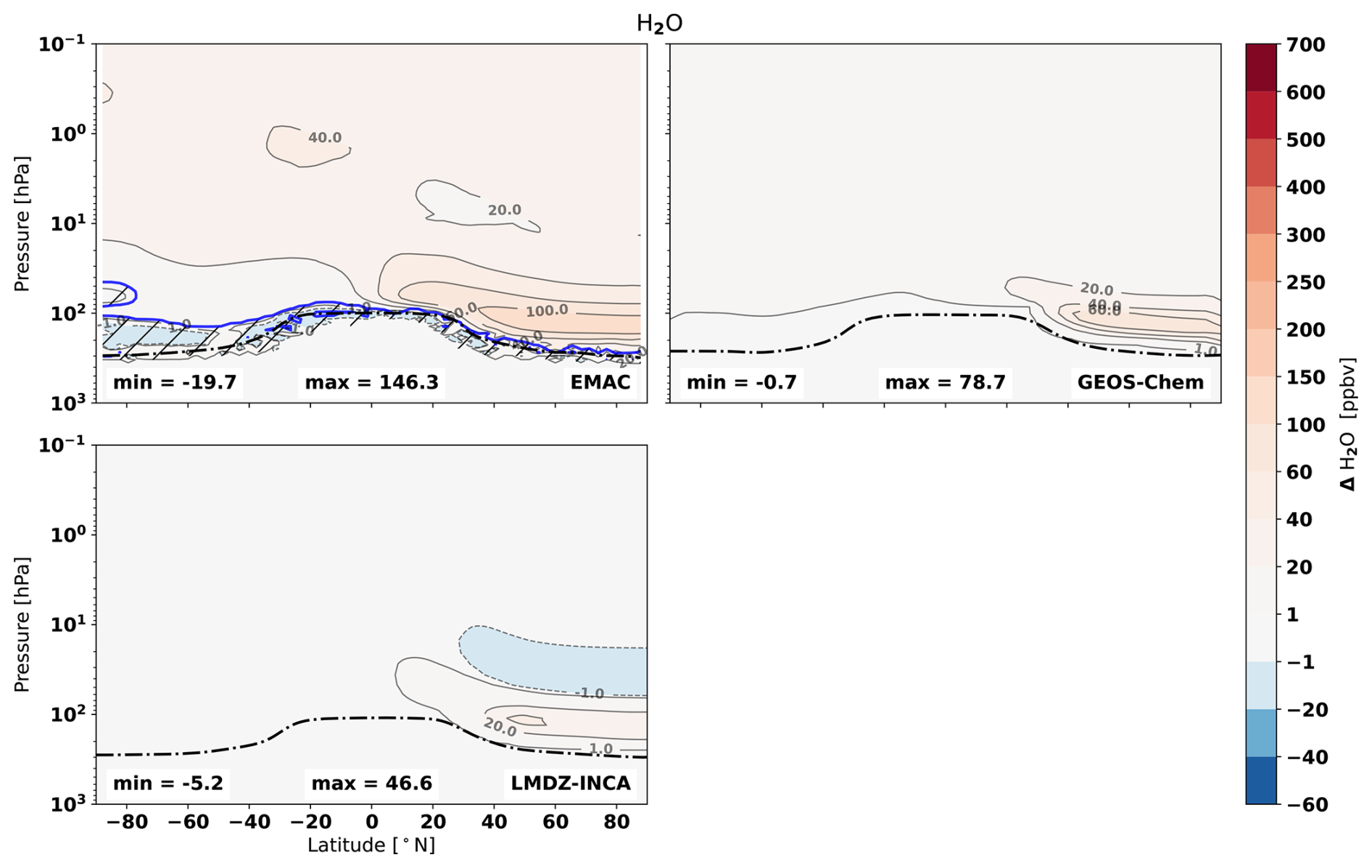
Figure A4 Changes in H₂O volume mixing ratios for the low-cruise (S3) emission scenario. Hatched areas enclosed by blue lines indicate regions that are not statistically significant for the EMAC results. Dashed–dotted lines show the mean tropopause pressure that is calculated per model.

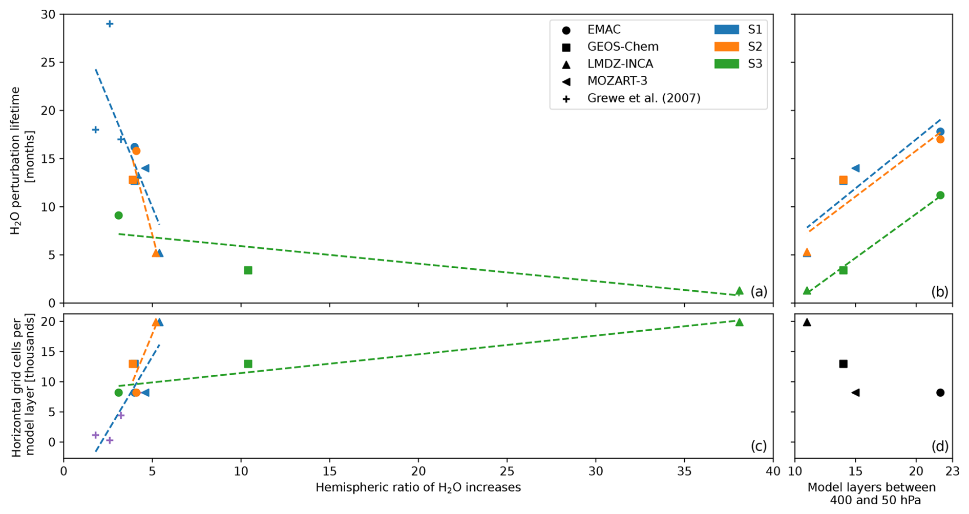
Figure A5 Comparison of the H₂O perturbation lifetime in months and the hemispheric ratio of the H₂O increases in the nominal supersonic scenario (S1) with vertical and horizontal model grid characteristics. Panel (a) shows the relationship between the perturbation lifetime and the hemispheric ratio, panel (b) shows the perturbation lifetime and the number of grid layers between 400 and 50 hPa, and panel (c) shows the hemispheric ratio and the horizontal grid fidelity. Panel (d) shows the number of grid layers between 400 and 50 hPa against the horizontal grid fidelity. Markers denote the different models and colors different scenarios. Results from Grewe et al. (2007) are included for their S1-equivalent SST scenario (S5 in Grewe et al., 2007).

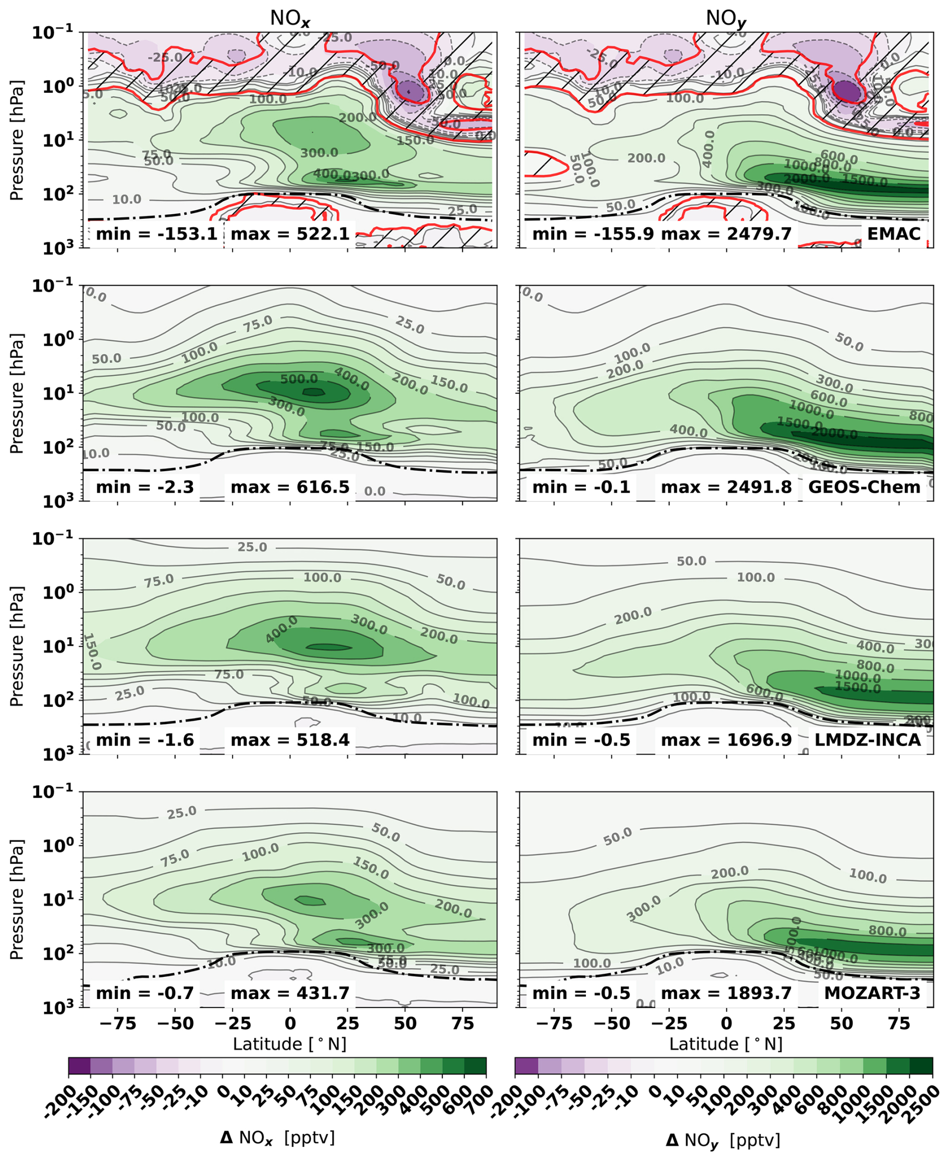
Figure A6 Mean changes in NO_x (left) and NO_y (right) concentrations in the triple-NO_x (S2) emission scenario across the models. Hatched areas enclosed by red lines indicate regions that are not statistically significant for the EMAC results. Dashed–dotted lines show the mean tropopause pressure that is calculated per model.

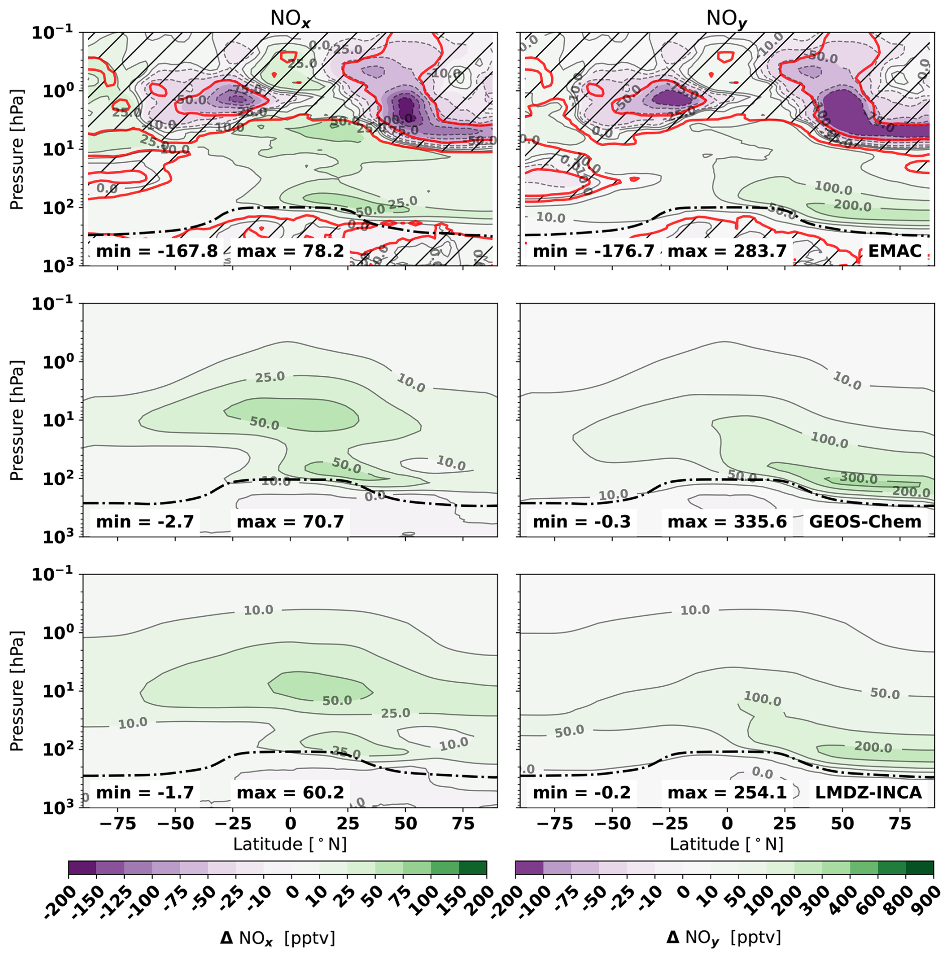
Figure A7 Same as Fig. A6 but for the low-cruise (S3) scenario. Hatched areas enclosed by red lines indicate regions that are not statistically significant for the EMAC results. Dashed–dotted lines show the mean tropopause pressure that is calculated per model.

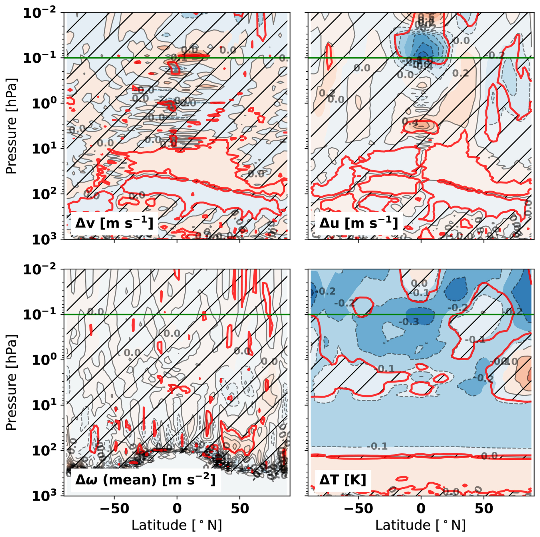
Figure A8 Changes in mean wind speeds ($v,u,\mathit{\omega }$) and temperature (T) in EMAC in response to the nominal supersonic emission scenario (S1). Hatched areas enclosed by red lines are not statistically significant over the 6-year evaluation period. Positive changes in u indicate increased eastwards velocities; the positive direction in v is northward, whereas Δω shows changes in vertical acceleration.

Figure A9 Same as Fig. A8 but for the triple-NO_x emission scenario (S2).

Figure A10 Same as Fig. A9 but for the low-cruise scenario (S3).

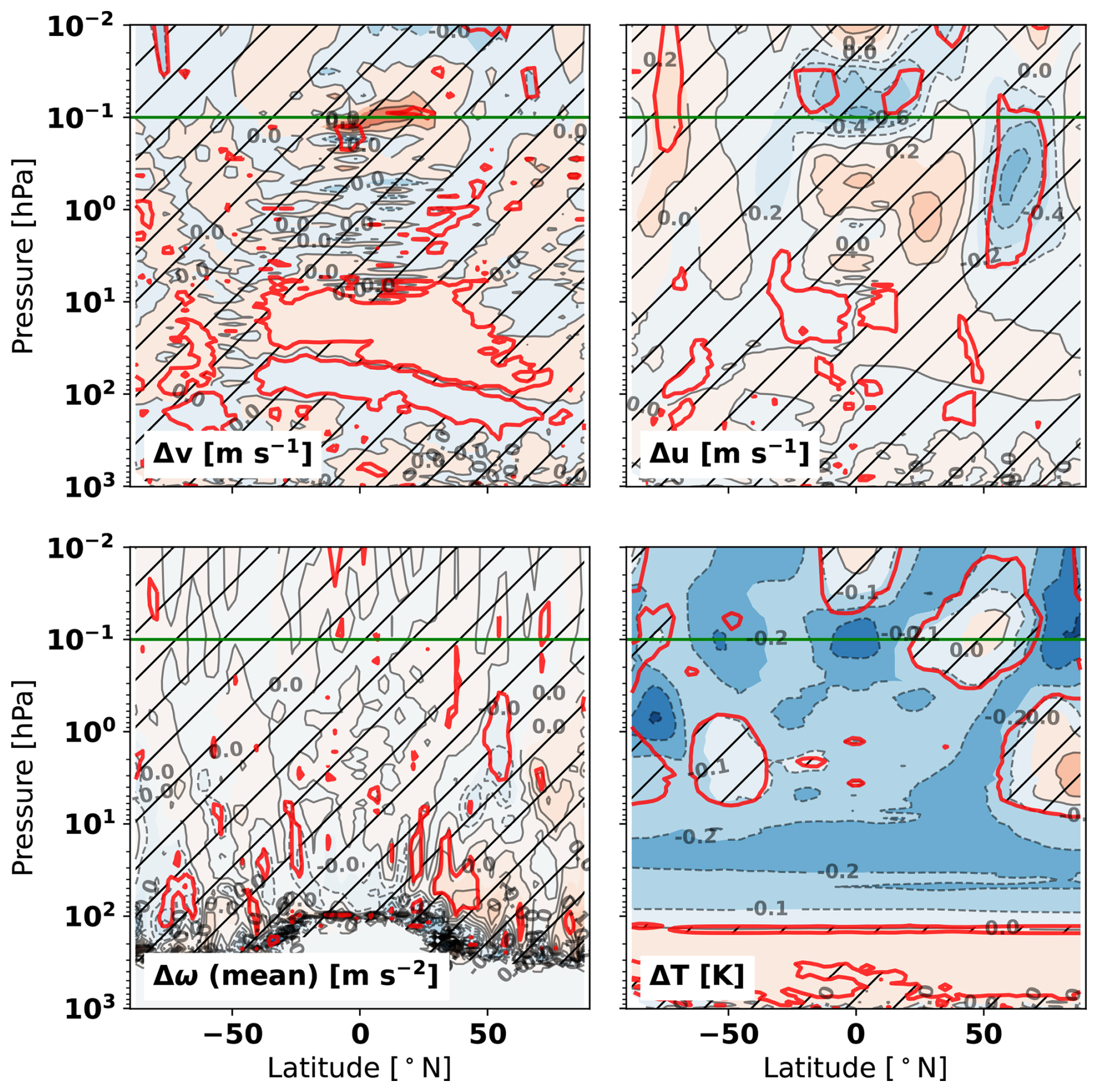
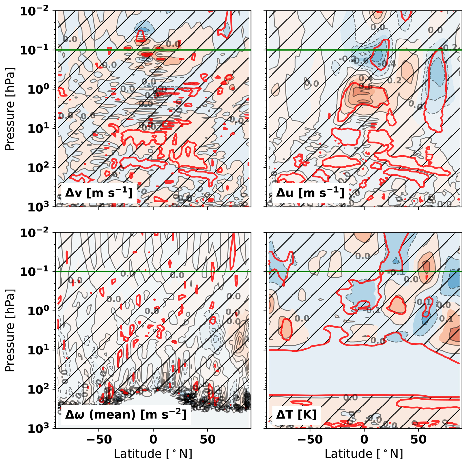
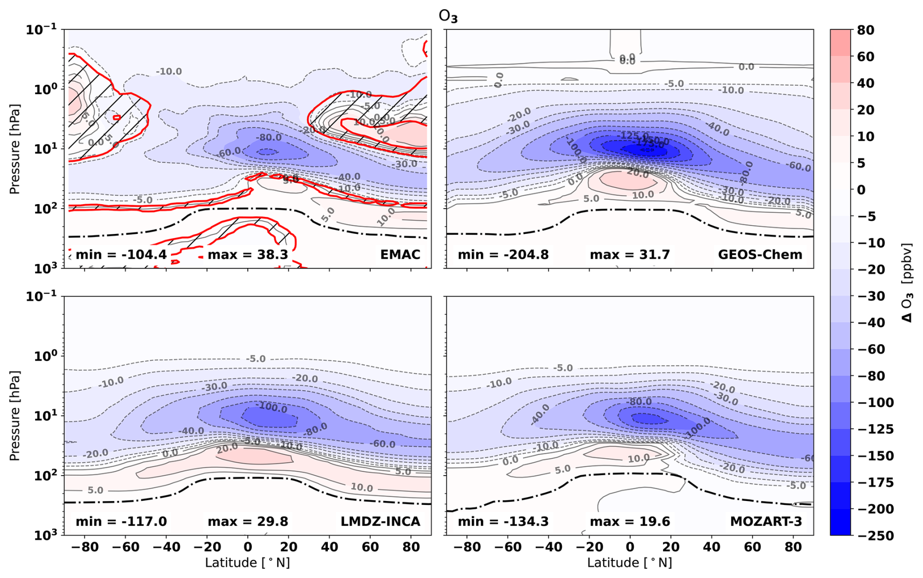
Figure A11 Changes in the ozone volume mixing ratio (VMR) for the triple-NO_x (S2) emission scenario. Hatched areas enclosed by red lines indicate regions that are not statistically significant for the EMAC results. Dashed–dotted lines show the mean tropopause pressure that is calculated per model.

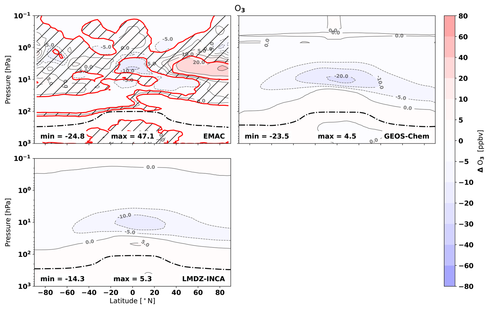
Figure A12 Similar to Fig. A11 but for the low-cruise (S3) scenario. Hatched areas enclosed by red lines indicate regions that are not statistically significant for the EMAC results. Dashed–dotted lines show the mean tropopause pressure that is calculated per model.

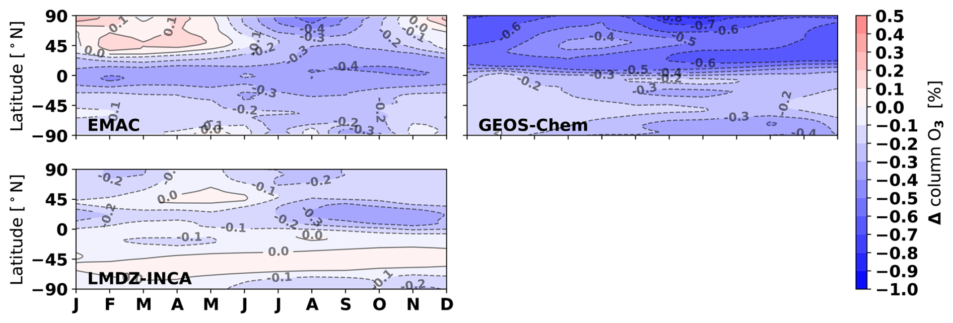
Figure A13 Mean monthly changes in the ozone columns (in percentage) in response to the triple-NO_x emissions (S2–S0).

Figure A14 Similar to Fig. A13 but for the low-cruise (S3) scenario.

Figure A15 Same as Fig. 8 but for the triple-NO_x (S2) emission scenario.

Figure A16 Same as Fig. 8 but for the low-cruise (S3) emission scenario.

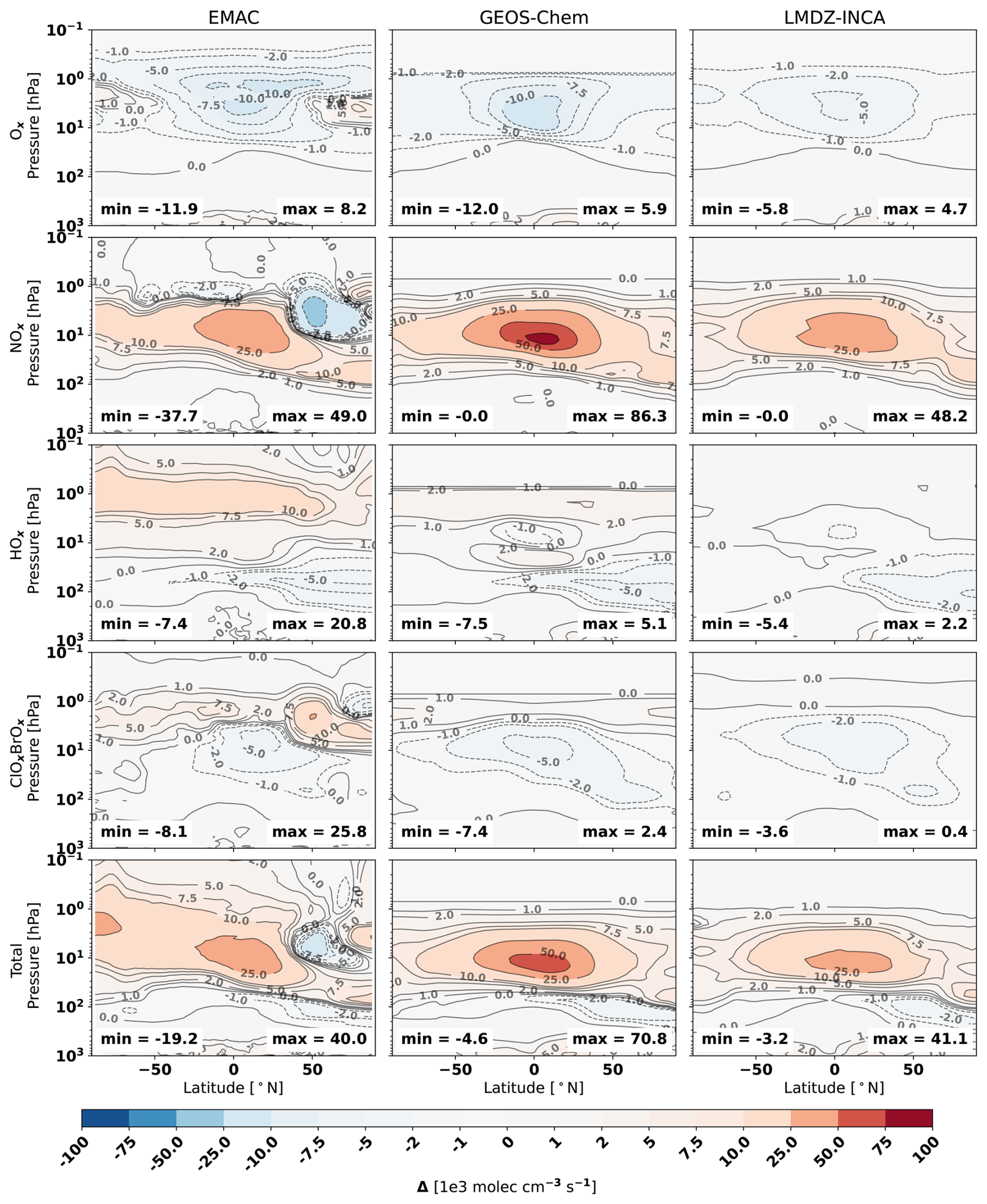
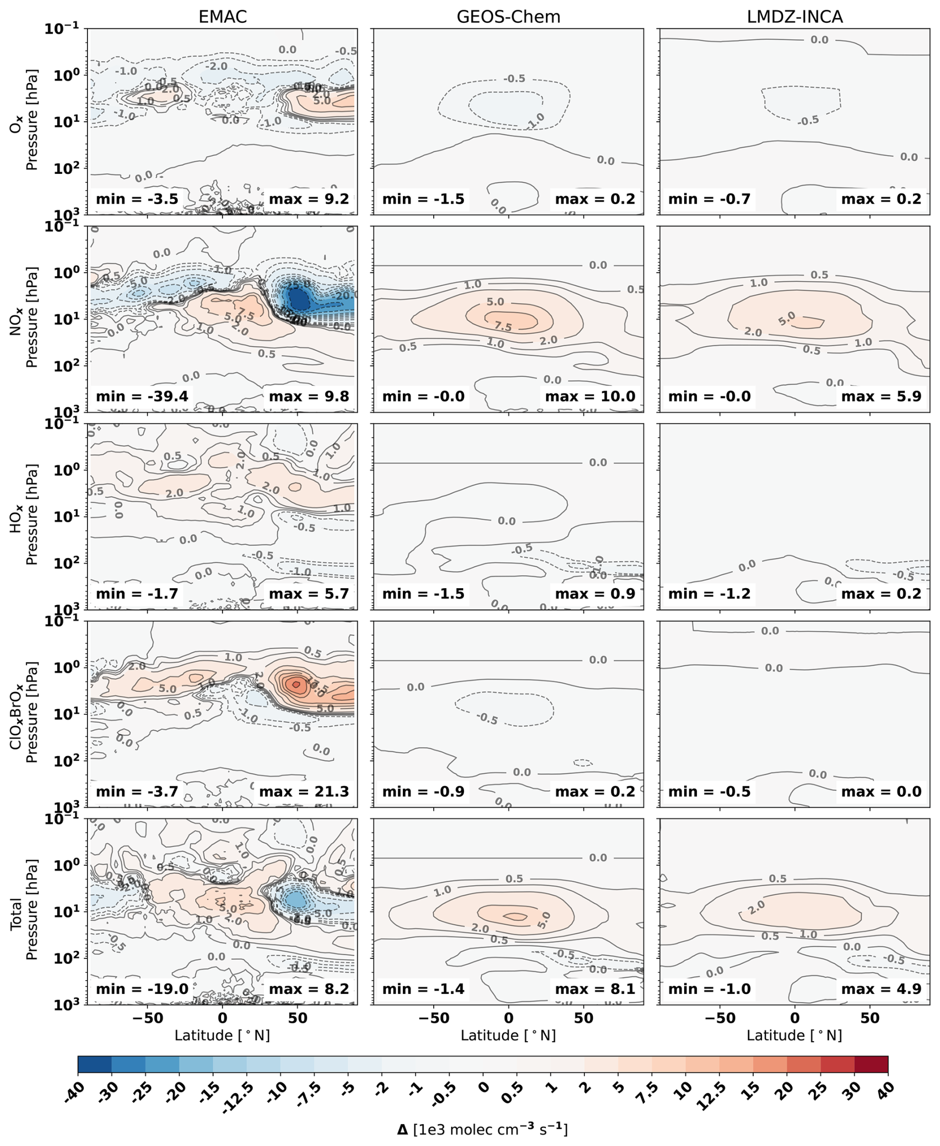
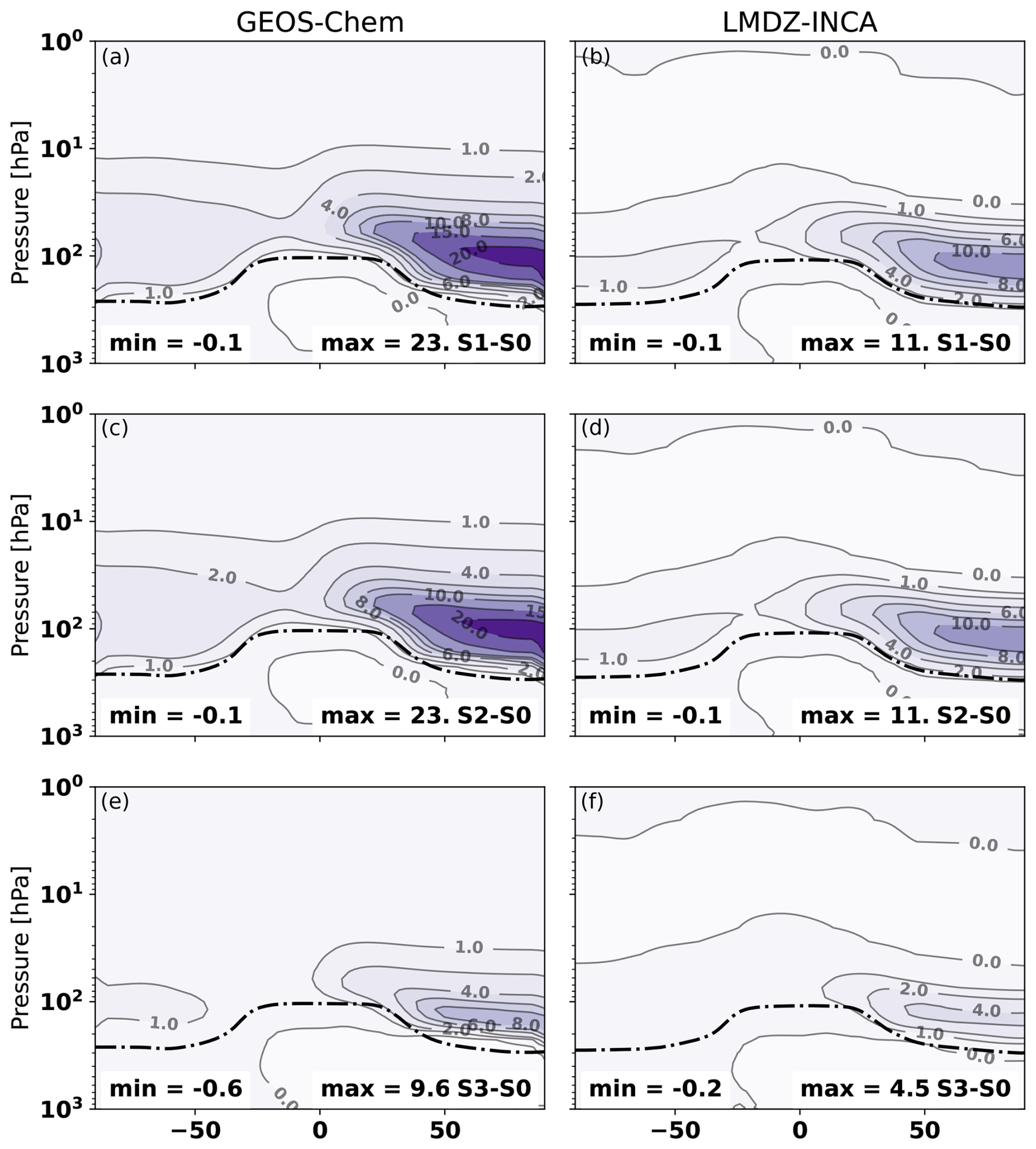
Figure A17 Comparison of the black carbon aerosol perturbations in 10⁻² ng m⁻³ for GEOS-Chem (a, c, e) and LMDz–INCA (b, d, e).

Figure A18 Comparison of the SO₄ aerosol perturbations in ng m⁻³ for GEOS-Chem (a, c, e) and LMDz–INCA (b, d, e).

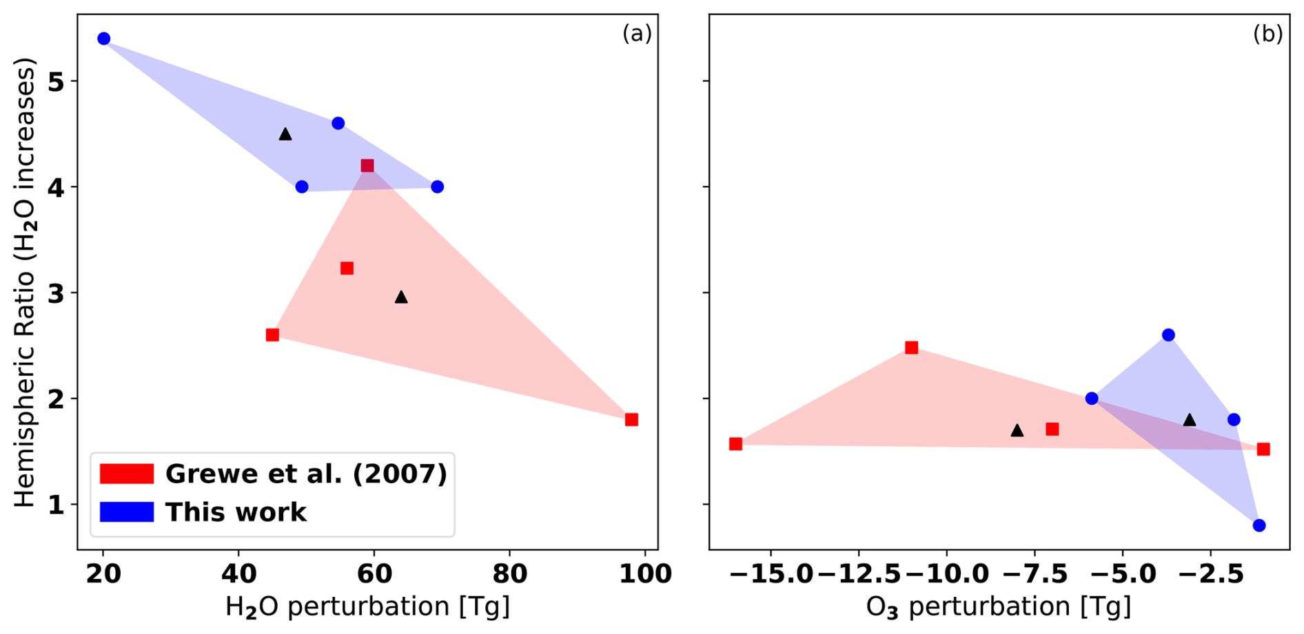
Figure A19 Comparison of the H₂O (a) and O₃ (b) perturbations and hemispheric ratios for the models used in this work and Grewe et al. (2007). Black triangles represent the multi-model means.